State Monitoring Method for Tool Wear in Aerospace Manufacturing Processes Based on a Convolutional Neural Network (CNN)

Abstract

In the aerospace manufacturing field, tool conditions are essential to ensure the production quality for aerospace parts and reduce processing failures. Therefore, it is extremely necessary to develop a suitable tool condition monitoring method. Thus, we propose a tool wear process state monitoring method for aerospace manufacturing processes based on convolutional neural networks to recognize intermediate abnormal states in multi-stage processes. There are two innovations and advantages of the proposed approach: one is that the criteria for judging abnormal conditions are extended, which is more useful for practical application. The other is that the proposed approach solved the influence of feature-to-recognition stability. Firstly, the tool wear level was divided into different state modes according to the probability density interval based on the kernel density estimation (KDE), and the corresponding state modes were connected to obtain the point-to-point control limit. Then, the state recognition model based on a convolutional neural network (CNN) was developed, and the sensitivity of the monitoring window was considered in the model. Finally, open-source datasets were used to verify the feasibility of the proposed method, and the results demonstrated the applicability of the proposed method in practice for tool condition monitoring.

1. Introduction

In recent years, with the rapid improvement of social technology, mechanical parts have gradually become more complex and sophisticated to meet the increasing needs of advanced manufacturing industries, such as the aerospace industry, but this has brought challenges to ensuring the reliability for existing monitoring methods [1]. For products in the aerospace industry, if a key precision component fails, the resulting damage can be unpredictable, not only causing loss of personnel and property, but even affecting the development of the entire industry. Therefore, compared with other industries, the aerospace industry has a stronger demand for high-quality parts [2,3]. The manufacturing stage is extremely important to the aerospace industry. According to the statistics, most of the early failures of aerospace components are caused by the surface defects of mechanical components. These defects mainly come from the manufacturing process, such as burrs, roughness, and shape errors [4]. The tool directly contacts the workpiece, and tool wear increases the surface roughness of the workpiece and reduces the quality of the workpiece [3,5]. Severe types of tool wear can cause chipping, cracking, and chattering, which can damage the workpiece and machine tool, leading to serious processing faults; thus, it is necessary to ensure the normal use of the part aerospace component [6,7,8].

The most primitive TCM method is that the operator estimates the process condition by the processing noise, chip shape, or cutting vibration differences. This method completely relies on the operator’s own experience, which is inefficient and difficult to meet the requirements of complex processes [9,10]. In the manufacturing process, with the development of related fields in the past few decades, many TCM methods have been proposed and developed. For example, part of the work attempted to monitor abnormal conditions based on physical models [11,12]. However, the physical model is often very complicated. Another piece of research began with the popular image recognition idea in recent years [13], which, by capturing tool images, analyzes tool-wear states based on digital image processing [14]. However, the monitoring accuracy of this method is easily affected by light and physical monitoring angles [15].

Most popular research is based on data-driven methods [16,17], which usually compare health index changes under normal and fault conditions for monitoring [18,19]. Fault monitoring is generally implemented based on fault detection indicators exceeding a certain threshold. Under the guidance of this idea, many studies have been established based on the idea of statistical process control (SPC) [20,21,22]. Additionally, control charts play an important role for SPC, which can judge whether the machining process is under controlled and improve the quality level to obtain a more satisfactory product quality [23]. The earliest control chart is the Shewhart control chart, but it is not sensitive to small quality parameters [24]. In order to solve its drawbacks, researchers have developed the CUSUM (cumulative sum control) and EWMA (exponential weighted moving averages) chart [25,26,27,28,29]. However, these control charts are still only post-analysis control methods; most of the established control limits consider, to a lesser extent, the stage characteristic of the process, which cause shortcomings for timeliness and cannot accurately judge or respond to abnormal conditions immediately [30]. For the tool wear process, it has a relatively obvious stage. The traditional monitoring method is more complicated and needs to be processed in stages to ensure better results. In addition, the recognition effect often depends on the quality of the extracted features for data-driven method, so the recognition effect is unstable [31,32]. Therefore, in order to make up the shortcomings of the above methods, a new tool wear process state monitoring method based on CNN (convolutional neural network) is proposed [15,33]. Firstly, the tool wear level was divided into different state modes according to the probability density interval based on the kernel density estimation (KDE), and the corresponding state modes were connected to obtain the point-to-point control limit. Then, the state recognition model based on a convolutional neural network (CNN) was developed, and the sensitivity of the monitoring window was considered in the model. Compared with the traditional approach, the proposed approach in this paper has two main points of innovation and advantages.

(1) In this study, the control limits were transformed into a multi-level control limit that related to points. Compared with traditional approach, the proposed approach had better time-varying characteristics and was more suitable for multi-stage process monitoring. Additionally, it enriched the discrimination method of SPC.

(2) The built state recognition method was based on the CNN, which did not have a feature selection step. Compared with traditional data-driven method, the problem of dependence of features was overcome, and the sensitivity of the monitoring window was considered in the proposed model.

The rest of the article is arranged as follows: Section 2 introduces the basic theory and methodology of the proposed approach in detail. The research ideas and algorithm flow are introduced in Section 3. Section 4 discusses the validation of the proposed method with the PHM2010 datasets. The experimental results are discussed in Section 5. Finally, we present the conclusions of our work in Section 6.

2. Theory and Methodology

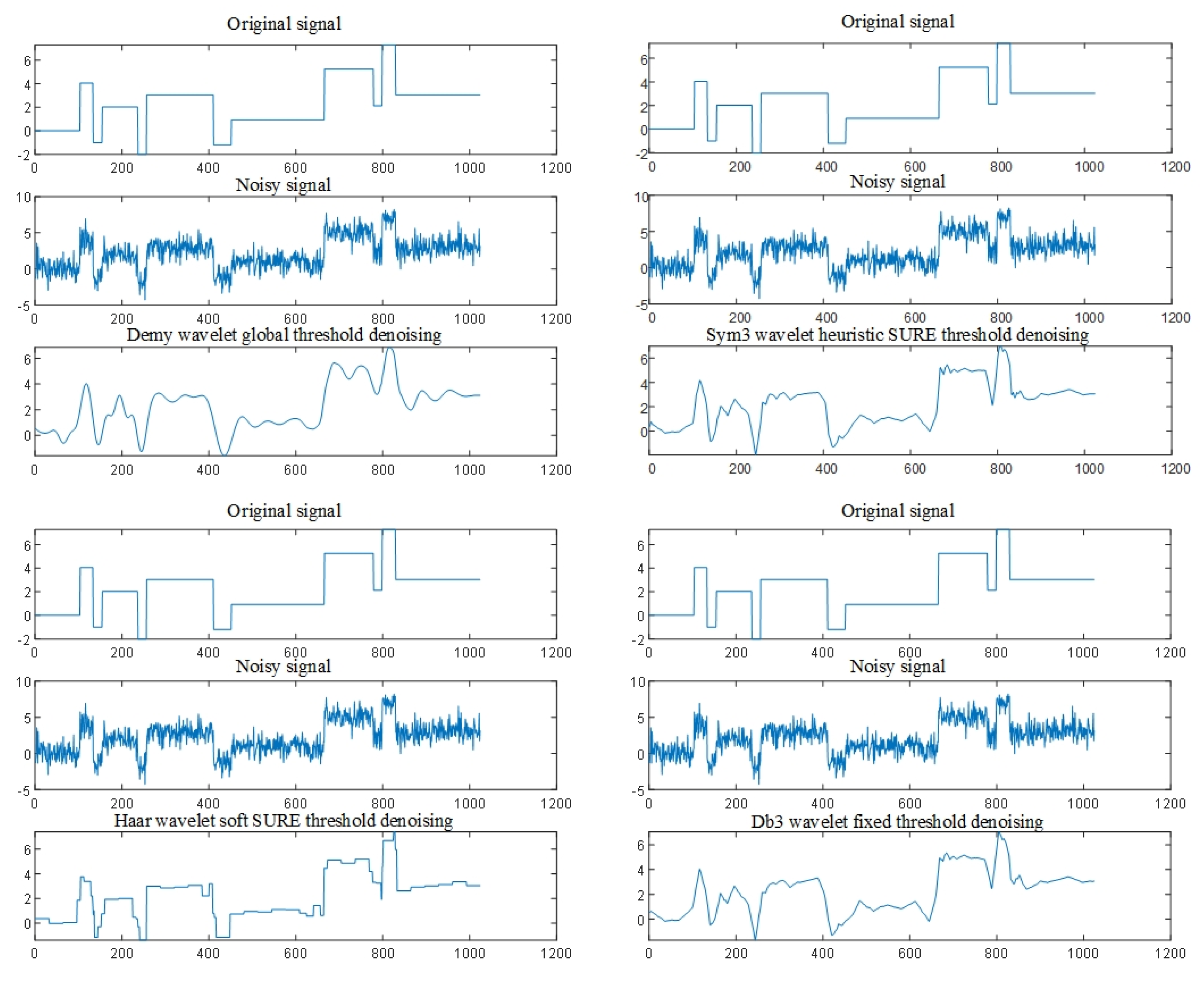
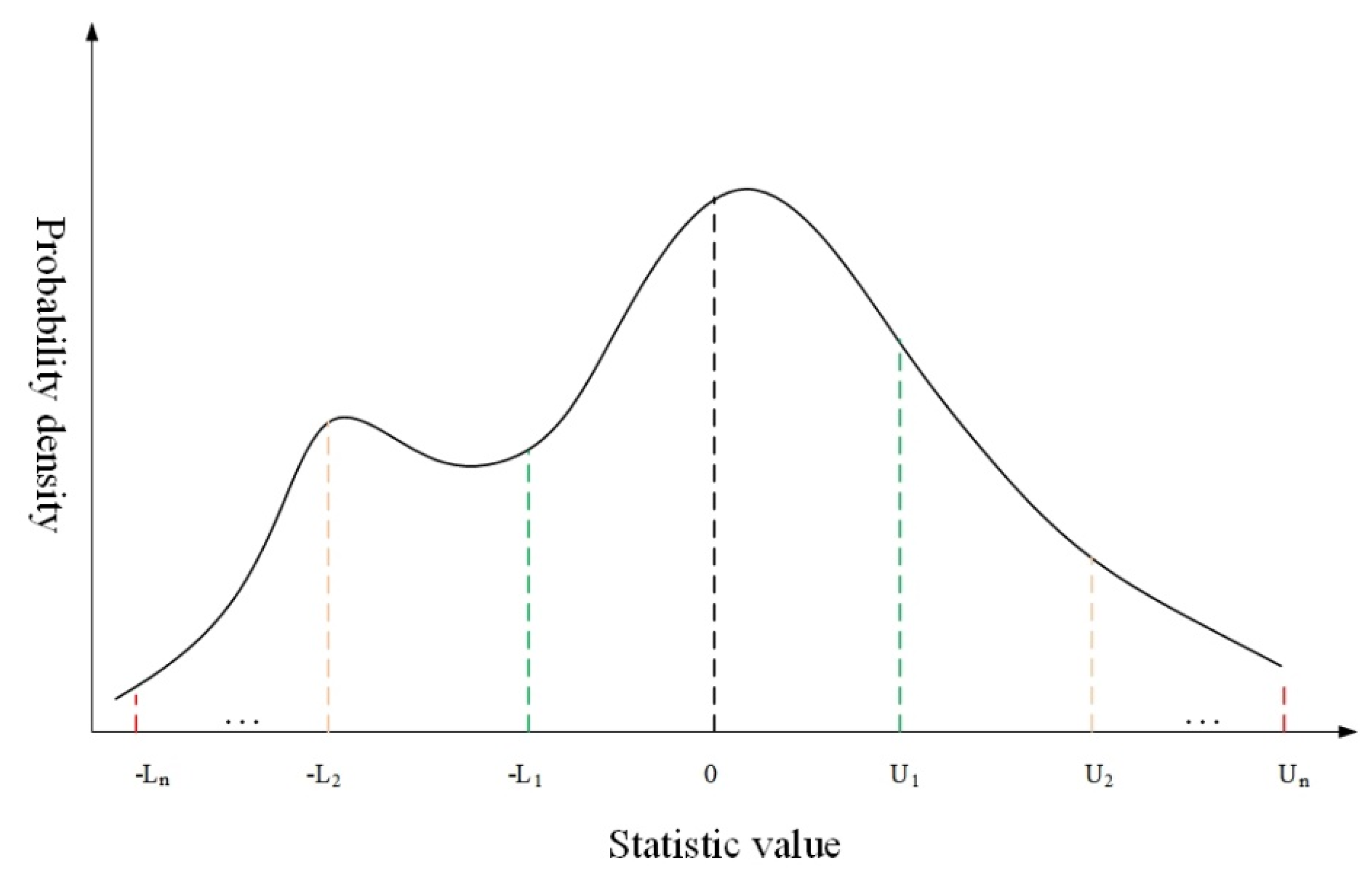
2.1. Kernel Density Estimation

In actual engineering applications, the collected data are often random, and their probability density is also in an unknown state, so the specific distribution form cannot be determined. In order to obtain the data distribution, we often fit the distribution according to the characteristics and properties of the data themselves. For the non-parametric estimation method, the most basic method is a histogram. However, the density function is not smooth and is greatly affected by sub-interval width for histograms [33], so in order to solve the shortcoming of the histogram, a method of kernel density estimation was proposed. As a non-parametric estimation method, kernel density estimation (KDE) is suitable for the absence of a priori distribution of data [34,35]. It can reflect the distribution of characteristic parameters under different fault states and different fault types. The independent and identically distributed F with n sample points (x₁, x₂, x₃, …, x_n) has the probability density function as f. The density estimation formula can be calculated as follows [36,37]:

$$\widehat{f}\left(x\right)=\frac{1}{n}{\displaystyle \sum _{i=1}^n{K}_h\left(x-x_i\right)}=\frac{1}{nh}{\displaystyle \sum _{i=1}^{n}K\left(\frac{x-x_i}{h}\right)}$$

(1)

Among them, h is the bandwidth, and h > 0, K is a non-negative function called the kernel function.

It can be seen from the formula that the most important thing is to determine K and h for KDE. The Gaussian kernel function is widely used, and the effect is good. Its can be calculated by Formula (2):

$$K(x)=\frac{1}{\sqrt{2\pi }}\exp \left(-\frac{1}{2}{x}^2\right)$$

(2)

The choice of bandwidth depends to a large extent on subjective judgment, and the choice of h can be achieved by using the minimized L₂ hazard function (mean integrated squared error). The definition of this function is:

$$MISE(h)=E{\displaystyle \int (\widehat{f}(}x)-f(x){)}^{2}dx$$

(3)

For the Gaussian kernel function used to estimate the kernel density, the result of h can be obtained by Formula (4).

$$h={\left(\frac{4{\widehat{\sigma }}^5}{3n}\right)}^{\frac{1}{5}}\approx 1.06\widehat{\sigma }{n}^{-\frac{1}{5}}$$

(4)

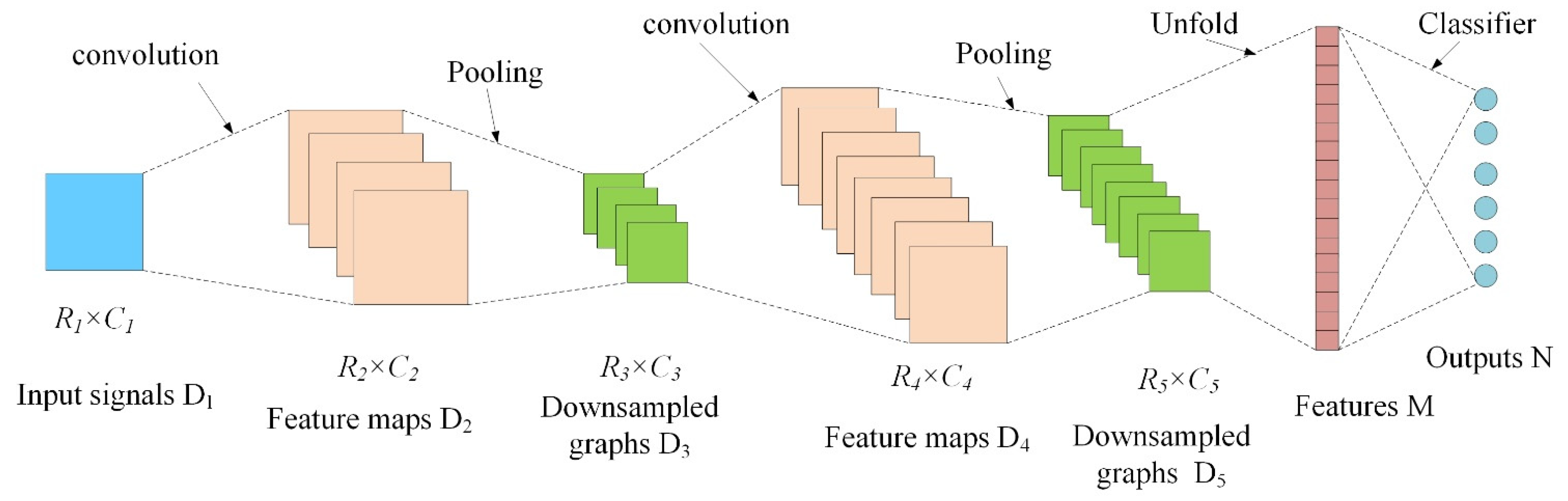
2.2. Convolutional Neural Network

As shown in Figure 1, three types of layers were used for the CNN, which were a convolutional layer, a pooling layer, and a fully connected layer. Therefore, a typical CNN structure can be divided into two parts: the convolutional layer and the pooling layer, which are used as feature extractors to implement feature extraction, and the fully connected layer is used as a classifier to implement pattern classification [38,39].

The weights and biases of the convolutional layer are organized into a series of convolution kernels (filters). The feature maps of the previous layer and the convolution kernel perform convolution operations and generate corresponding output feature maps. Among them, the convolution kernel will traverse the entire input feature maps with a fixed step size. Through this process, the parameters of the network are reduced, and the over-fitting phenomenon can be avoided. The weight adjustment algorithm of LMS learning rules is as follows:

$$x_j^{\prime }=f\left({\displaystyle \sum _{i=1}^{D_1-1}{x}_i^{I-1}}*{\omega }_{ij}^{\prime }+b_j^{\prime }\right),j=1,2,\dots ,D_1$$

(5)

where * represents the convolution operation, I represent the serial number of the current network layer, D is the number of feature maps, ω is the convolution kernel, x is the feature map, b is the bias matrix, and f is the activation function. The size of the feature map will change after passing through the convolutional layer. The size of the output feature map of the first convolutional layer is R and C, which can be obtained by Formula (6). R represents height, and C represents width.

$$R\times C_1=\left[\left(R_{-1}-r\right)/s+1\right]\times \left[\left(C_{I-1}-c\right)/s+1\right]$$

(6)

In the formula, r represents the height of the convolution kernel, c represents the width of the convolution kernel, and s represents the movement step length of the convolution kernel. After the convolution operation, the activation function will perform a nonlinear operation on its output. Commonly activation functions include Sigmoid and ReLU (Rectified Linear Unit). The two activation functions are, respectively, given by the following formulas:

$$f{(x)}_{\mathrm{Sigmoid} }=\frac{1}{1+e^{-x}}$$

(7)

$$f{(x)}_{\mathrm{ReLU} }=\max (0,x)$$

(8)

The pooling layer is used to reduce the dimensionality (down sampling) of the feature maps of the previous layer in order to quickly reduce the dimension. This achieves the purpose of effectively reducing the risk of over-fitting and reducing the calculation cost. The calculation process can be expressed as follows:

$$x_j^{\prime }=p\left(x_j^{I-1}\right),j=1,2,\dots ,D_1$$

(9)

In the formula, I represent the current network layer number, D represents the number of down-sampling graphs, x represents the feature graph, and p represents the down-sampling function [40]. Like the convolutional layer, the size of the feature map will also change after passing through the pooling layer. The calculation formula is as follows.

$$R\times C_1=\left(R_{-1}/u\right)\times \left(C_{I-1}/u\right)$$

(10)

The last is the fully connected layer. The fully connected layer expands and splices the elements in all the feature map matrices of the last layer of the network, and inputs them to the first fully connected layer. The number of neurons in this layer is M. The calculation formula is as follows.

$$M=R_{-1}\times C_{I-1}\times D_{I-1}$$

(11)

The neurons in the fully connected layers are completely connected to all the neurons in the previous layer, which can be expressed by Formula (12):

$$O=f\left({\omega }_0\cdot f_0+b_0\right)$$

(12)

Among them, f₀ is the eigenvector, ω₀ is the weight matrix, and b₀ is the bias vector.

The last layer is the output layer in CNN, which contains N neurons representing the number of pattern categories to be recognized. Usually, the activation function of the output layer is the Softmax function. Finally, in the training phase, the backpropagation algorithm is used to optimize the weights and biases in the CNN to minimize the cost. The loss functions are usually E₁ (Mean Squared Loss Function) and E₂ (Cross-entropy Loss Function), respectively. The calculation methods are as follows:

$$f{\left(x_1\right)}_{\mathrm{Sofmax} }=\frac{e^x}{{\displaystyle \sum _{j=1}^N{e}^{x_i}}}$$

(13)

$$E_1={\displaystyle \sum _{k=1}^N{\left(q_k^n-y_k^n\right)}^2}$$

(14)

$$E_2=-\frac{1}{N}{\displaystyle \sum _{k=1}^N{q}_k^n}\log y_k^n$$

(15)

$q_k^n$ represents the predicted value of the k-th dimension of the n-th sample, and $y_k^n$ represents the actual value of the k-th dimension of the n-th sample.

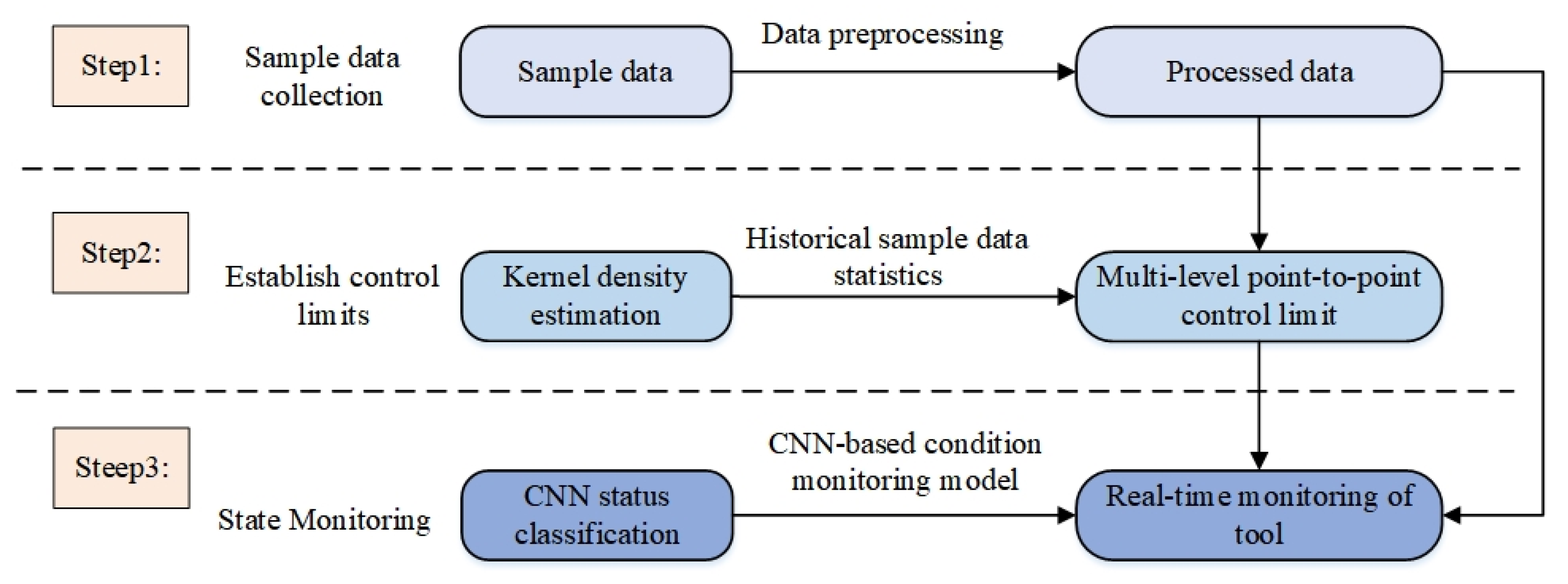
3. Proposed Approach Framework

The framework of the proposed approach is shown in Figure 2. As shown in Figure 2, the state monitoring method can be divided into three parts, which are the sample data collection, establishing the control limits, and the state monitoring. Some conventional data processing methods were implemented in first part. The core of the algorithm is in the second and third parts, which will be introduced in detail in the following sections.

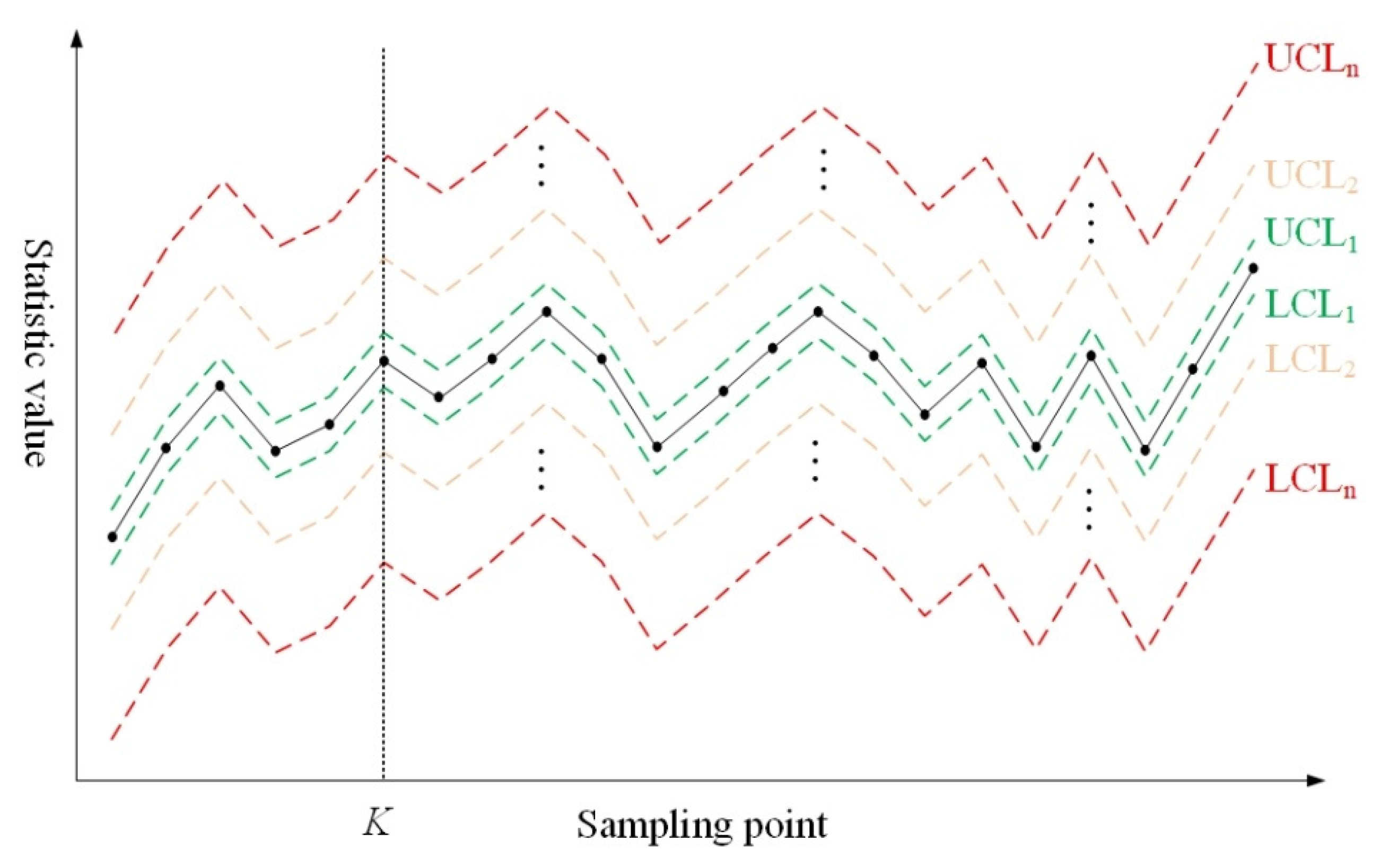
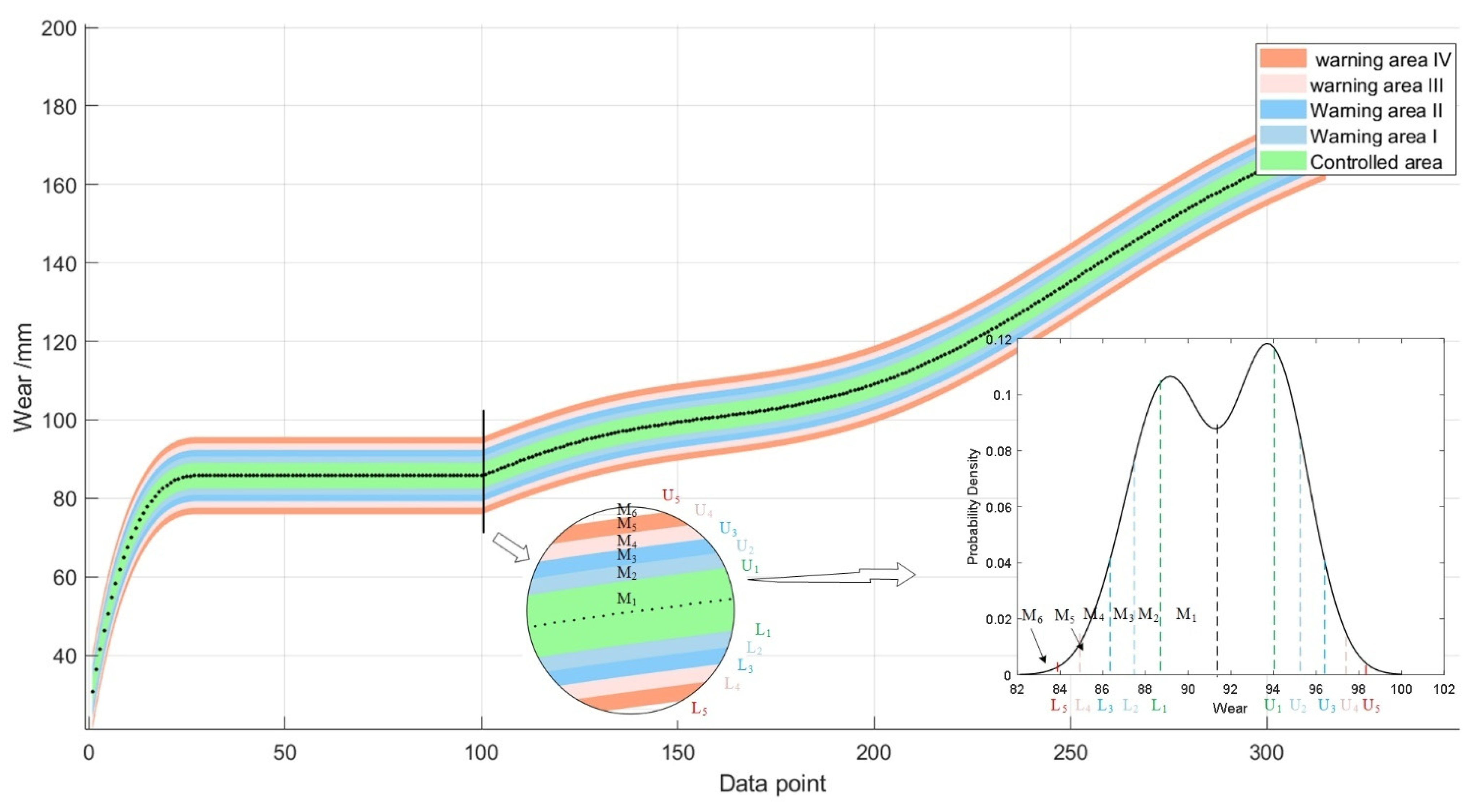
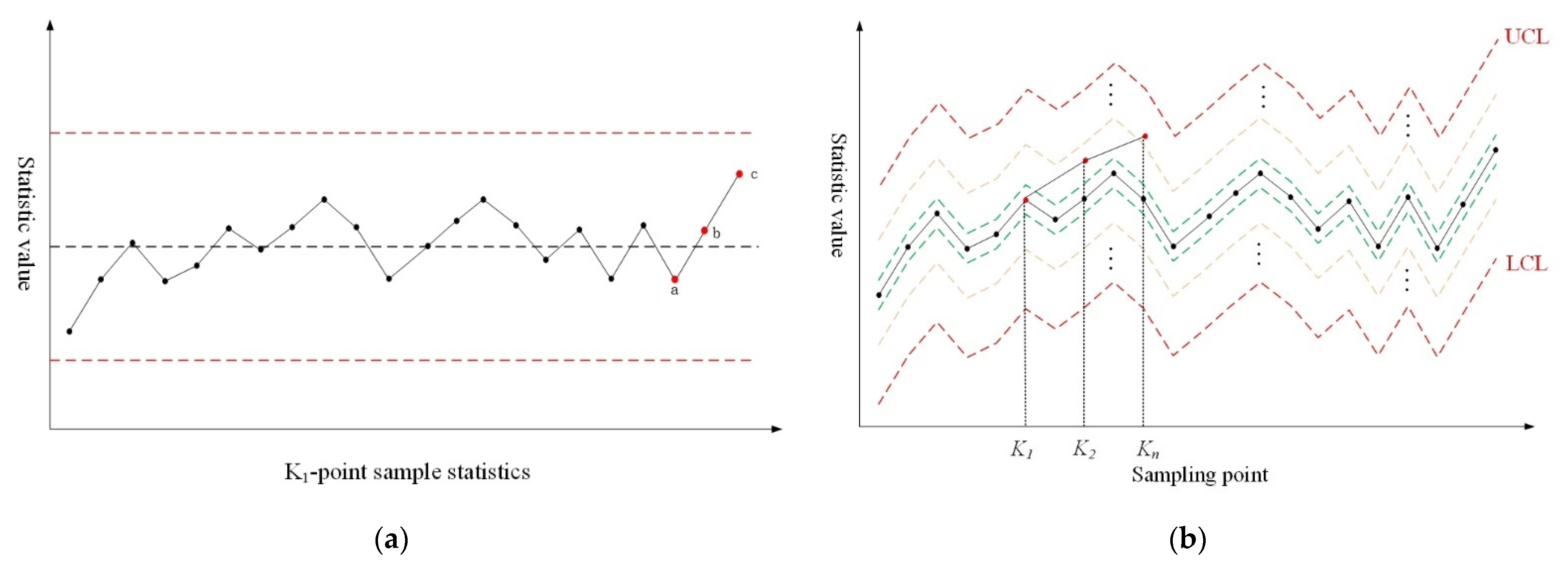
3.1. Construction of Point-to-Point Control Limit

As previously mentioned, the data-driven method is based on the monitoring index to distinguish normal and fault conditions. Thus, the idea based on SPC was introduced into this research. Additionally, the point-to-point control limit was established, and the point-to-point control limit mentioned here referred to the point-related control limit, which was obtained from a certain fixed processing process with a fixed sampling point to set the control limit. This control limit has better time-varying characteristics and is more sensitive in distinguishing abnormal states compared with the traditional approach. Further, in order to better evaluate the state of sampling point, the multi-level control limits were considered in the proposed approach by subdividing the identified level to better meet the actual needs.

The schematic diagram of the multi-level point-to-point control limit is shown in Figure 3. The state of the sampling point K was monitored by the n-level control limit. The different control levels represent the degree of deviation of the state at that point. The method of obtaining the multi-level control limits was by KDE, which was mentioned in Section 2.1. The Gaussian function was adopted as the kernel function, and the bandwidth h_M can be obtained based on MISE, which is shown as follows:

$$h_M=\min \left\{E{\left[{\displaystyle {\int }_{-\infty }^{+\infty }\left(\widehat{f}\left(x\right)-f\left(x\right)\right)}\right]}^{2}dx\right\}$$

(16)

Then the kernel density diagram of sampling point K can be obtained. As shown in Figure 4, the abscissa is the statistic value, and the ordinate is the probability density. Then, the multi-level control limit can be obtained by dividing probability at certain intervals. The state between the control limits can be set as different wear modes. The real-time of the modes can be classified by the algorithm to realize state monitoring.

3.2. Condition Monitoring Method Based on CNN Algorithm

After the control limit is completed, in order to monitor the real-time cutting process, it is necessary to judge whether the current tool wear state is under the control limit range or not. Therefore, this research proposes a condition monitoring method based on a CNN algorithm. In this method, all data are calculated in an observation window and then input into a CNN model to obtain the current cutting state.

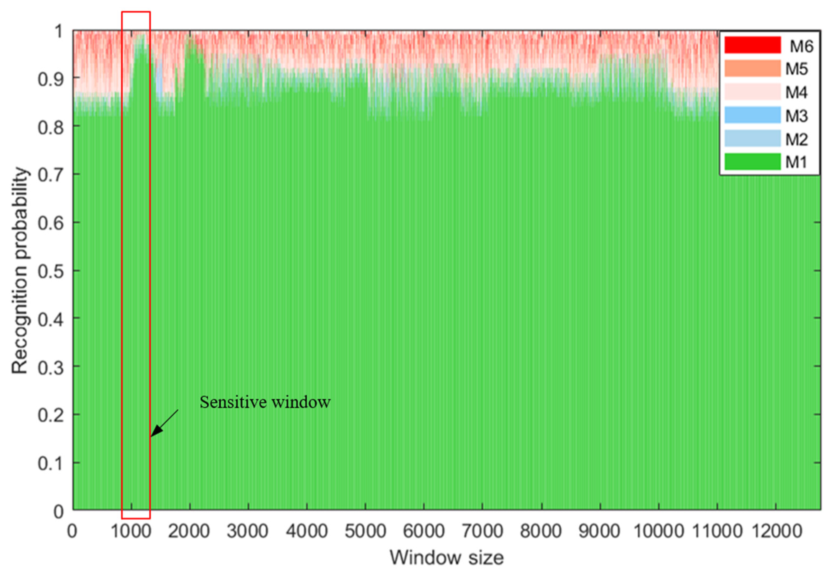
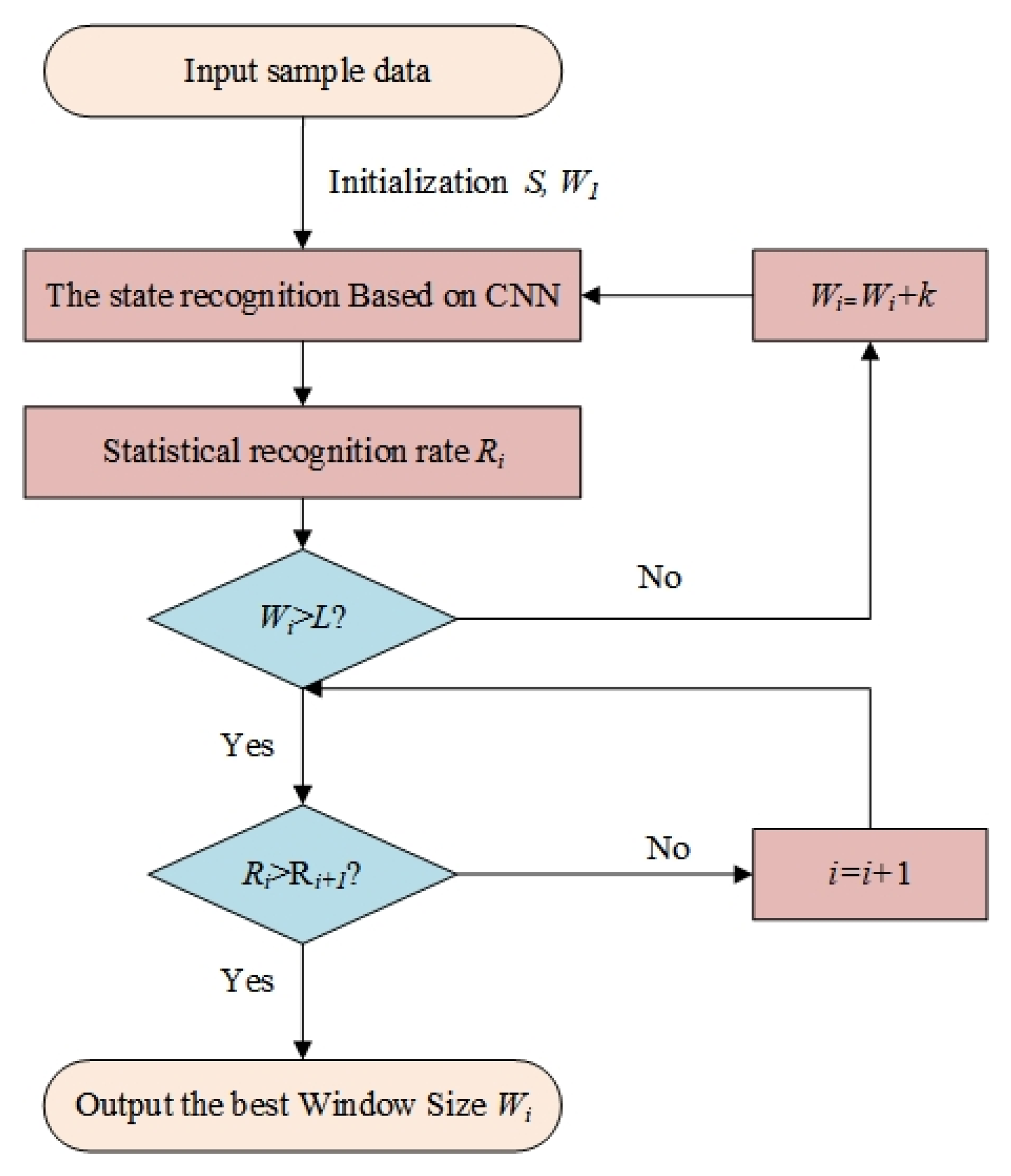
3.2.1. Optimal Sampling Window Determination

In real-time state recognition, previous research has shown that the recognition accuracy based on signal data is affected by the amount of data processed in a single timeframe, which is to say the recognition rate under different windows [41]. Therefore, it is necessary to test the recognition ability of the classification model under different observation windows and obtain the best window (or sensitive window). The process of window recognition test is shown in Figure 5. For tool wear process signal L, the window size was set as W, and the window moving step was set as S. Firstly, we initialized the window size as W = W₁ and then split the original signal under the window of W₁, and the CNN algorithm was used to identify and obtain the result. Then, we increased the window size W_i = W₁ + K, (K is the increase in window size), and the same method was used to test again until W_i reached the maximum value (the maximum value cannot be greater than the data size L). For example, if a sample signal L with 1000 data points was recognized, and the window moving step S = 1, then when W_i = 10, the classification model will recognize the sample 991 times. When W_i = 20, it will be identified 981 times, until W_i reaches the maximum value. After the CNN algorithm was tested under observation windows of all sizes, we counted the proportion of the identified states to obtain the recognition rate R_i and selected the observation window W, which corresponded to the highest recognition rate as the best window.

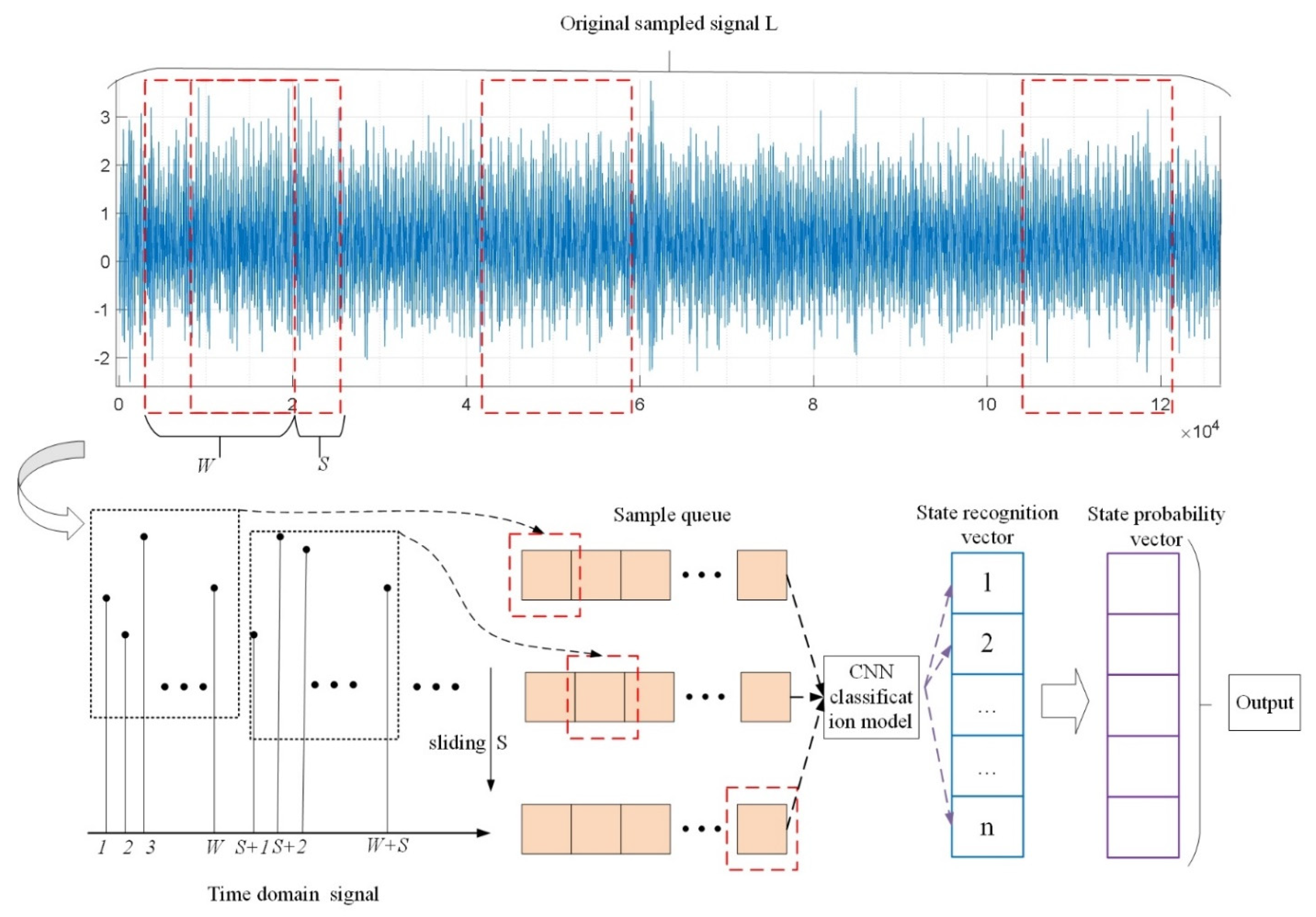
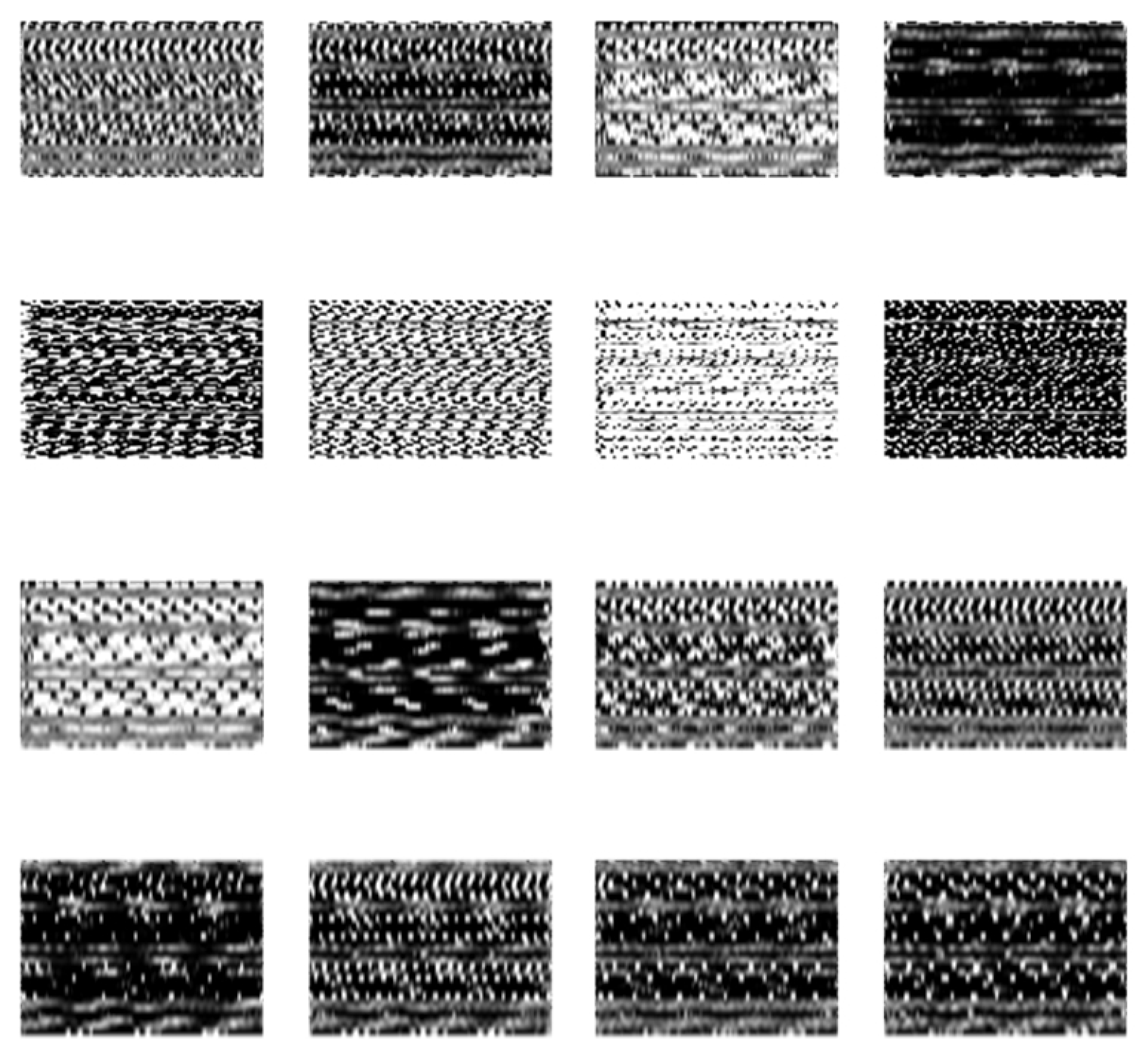
3.2.2. Mobile Sliding Window for State Recognition

After the optimal identification window size W was determined, we carried out the real-time tool state monitoring by a sliding window and combined it with the multi-level control limit proposed in Section 3.1. The process is shown in Figure 6.

For the real-time signal of the tool wear process, the data points L was used as the input feature vector. During the monitoring process, the sliding window size was S. As shown in Figure 6, the signal was divided into a sample queue with window size W and was identified by the CNN algorithm. The tool wear condition can be calculated by the CNN classification model. Assuming that there are n levels of control limits, the identified probability for each level can be obtained to make up the probability vector. Finally, the identification result with the highest probability level can be obtained as the output. According to the above method, it can be compared with the multi-level control limit mentioned in Section 3.1 to obtain the current tool wear state.

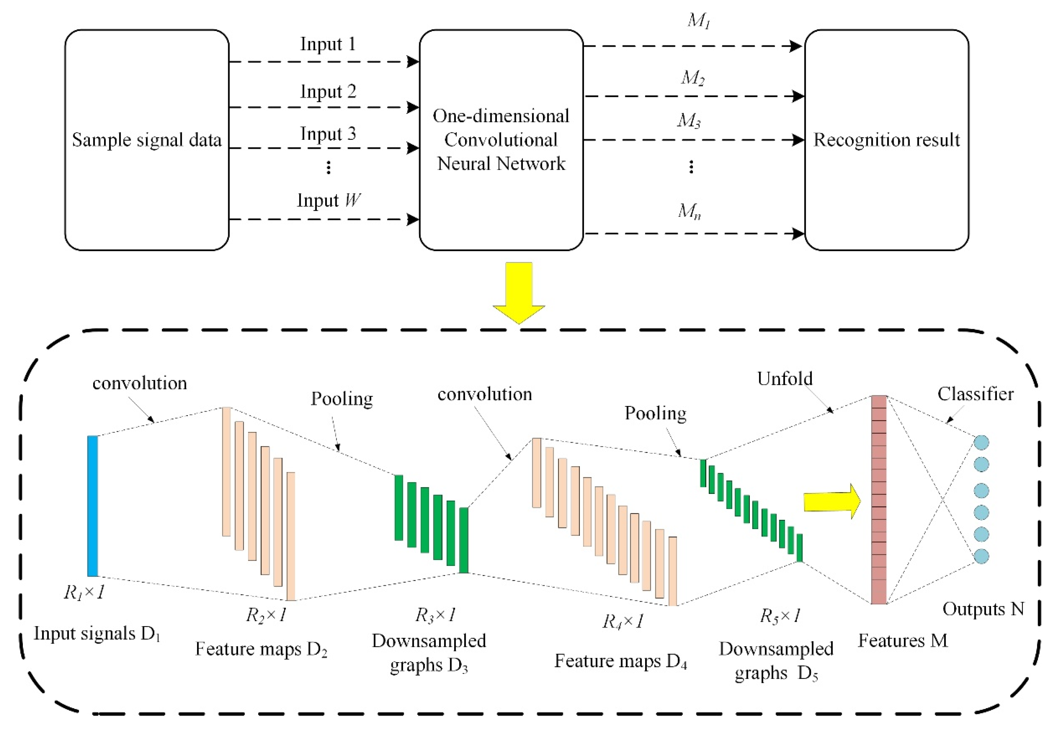
3.2.3. The Wear State Recognition Model with CNN

After the wear state recognition model, the core part is the CNN, which is used to judge the current condition of tool wear. In the traditional method, the feature extraction step is very important to affect the recognition accuracy for the classifier. However, it not only increased the workload and complexity of quality control, but the extracted features cannot be guaranteed to be optimal, which affected the stable performance of data-based condition monitoring methods [42]. The advantage of 1D-CNN (one-dimensional CNN) is that it can realize end-to-end recognition and diagnosis. The model input is raw data, and the output is the specific wear state. For CNN model, feature extraction, selection, and optimization are all conducted through alternating convolutional and pooling layers, and the idea of backpropagation is considered in the model. The algorithm optimizes and adjusts the weights and biases of CNN to minimize the loss function value, and then realizes adaptive feature extraction. This not only saved calculation costs, but is also more suitable in dealing with complex work. Additionally, the structure of 1D-CNN is slightly different from that of ordinary CNN. The feature map in its structure is not a matrix but a vector, which makes 1D-CNN more sensitive to time series samples such as vibration signals. The structure of the 1D-CNN used for condition recognition is shown in Figure 7.

From Figure 7, we can find that it consists of two alternating convolutional layers, two pooling layers, and a fully connected layer. According to the function in the CNN model described in Section 2.2, alternate convolutional layers, and pooling layers complete feature extraction, and then the fully connected layer implements state classification. Under the size of each window W, we input signal data R₁, then identified it as a certain category for the N-level control limit and then output it.

4. Experiment Verification

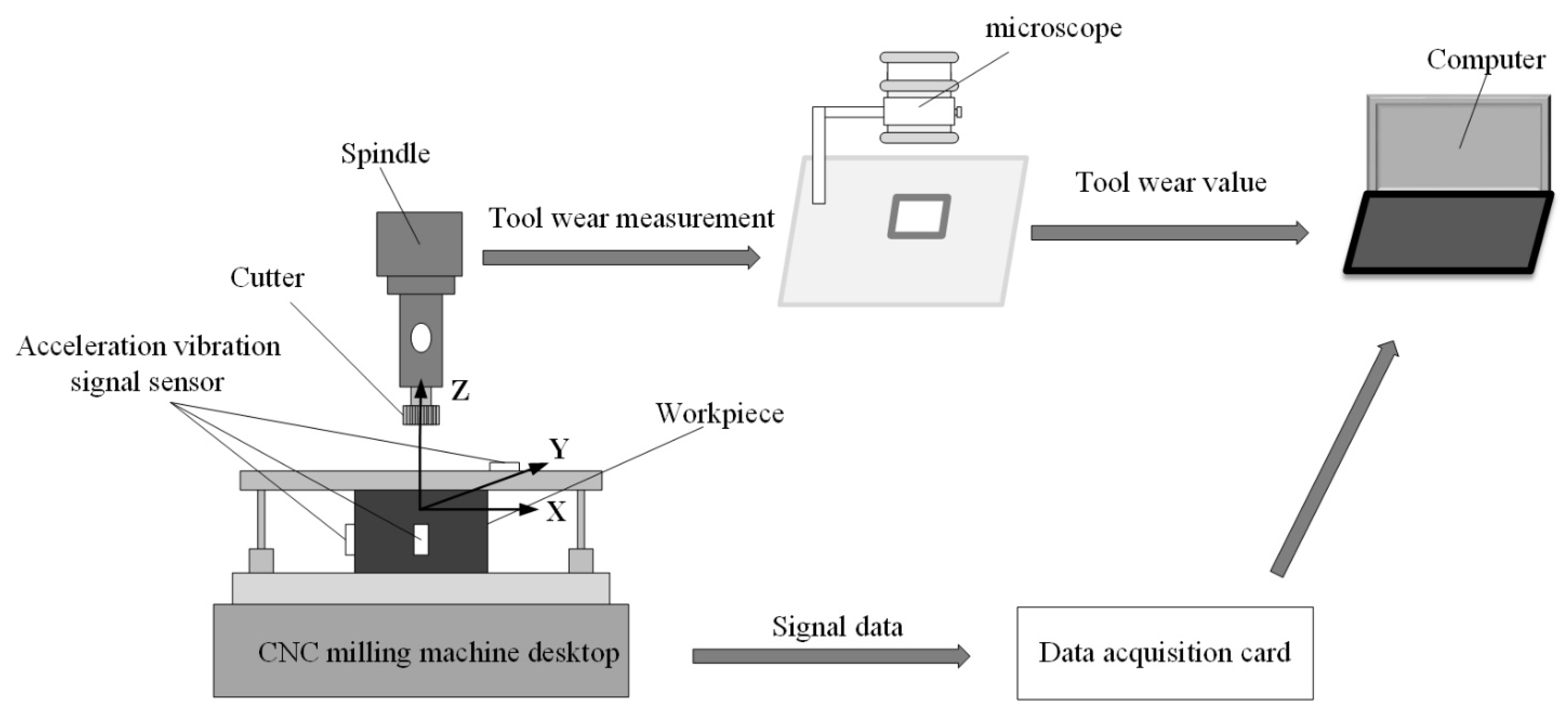
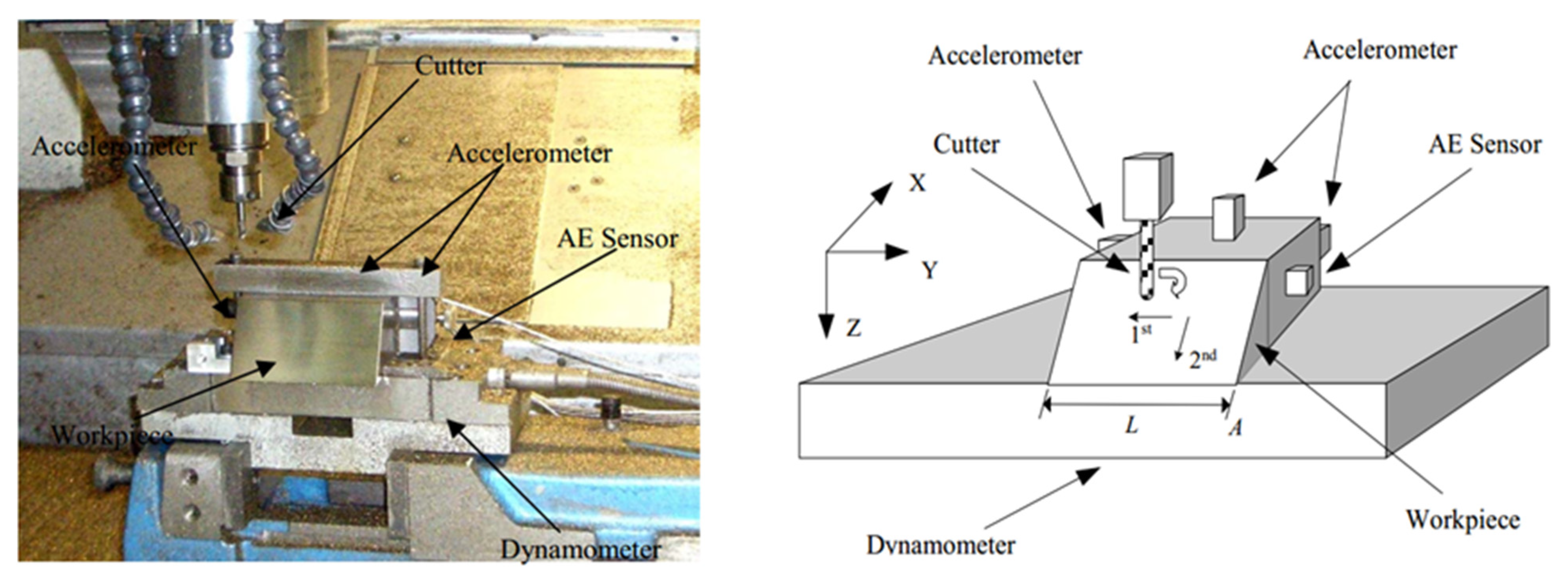
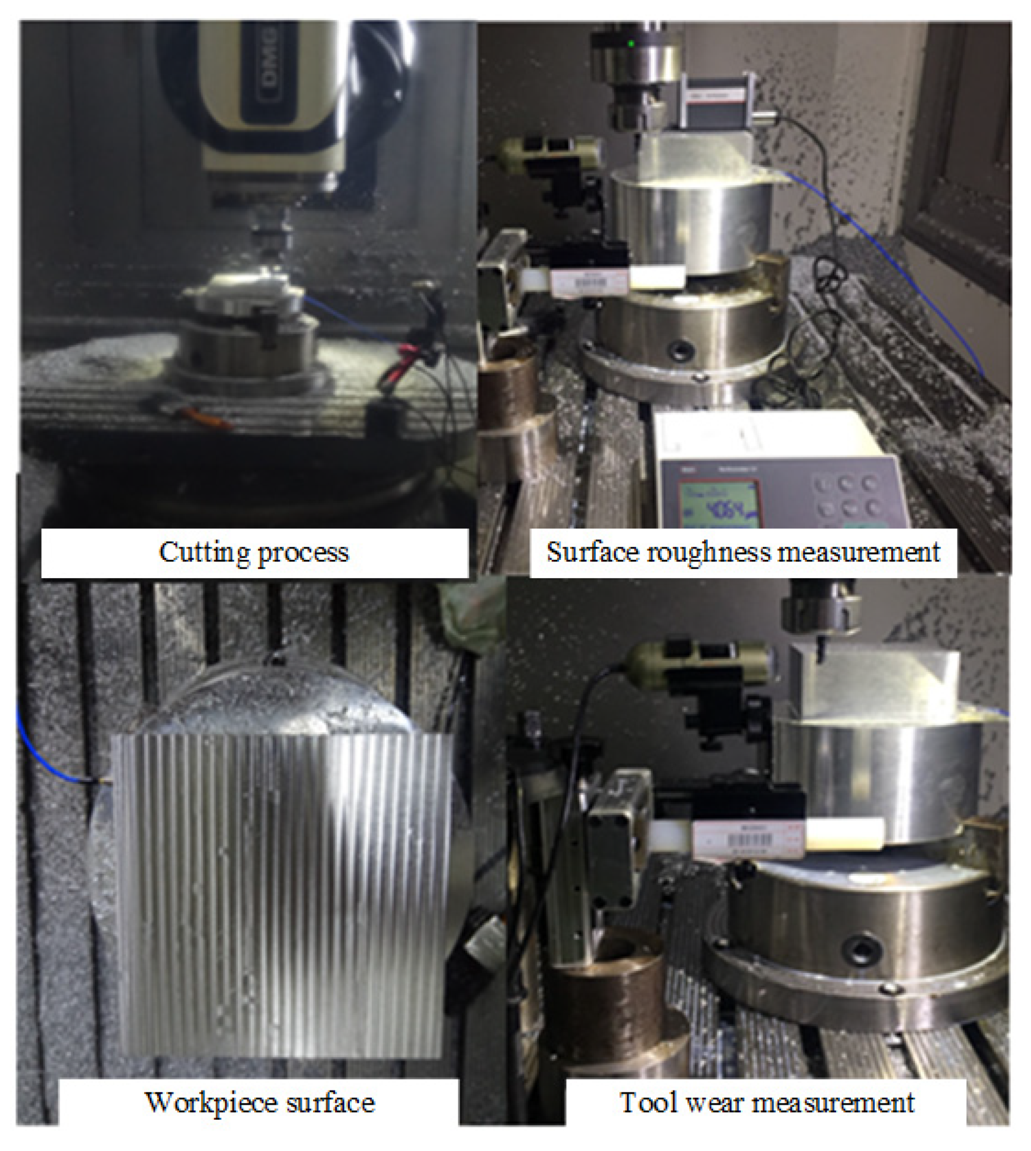
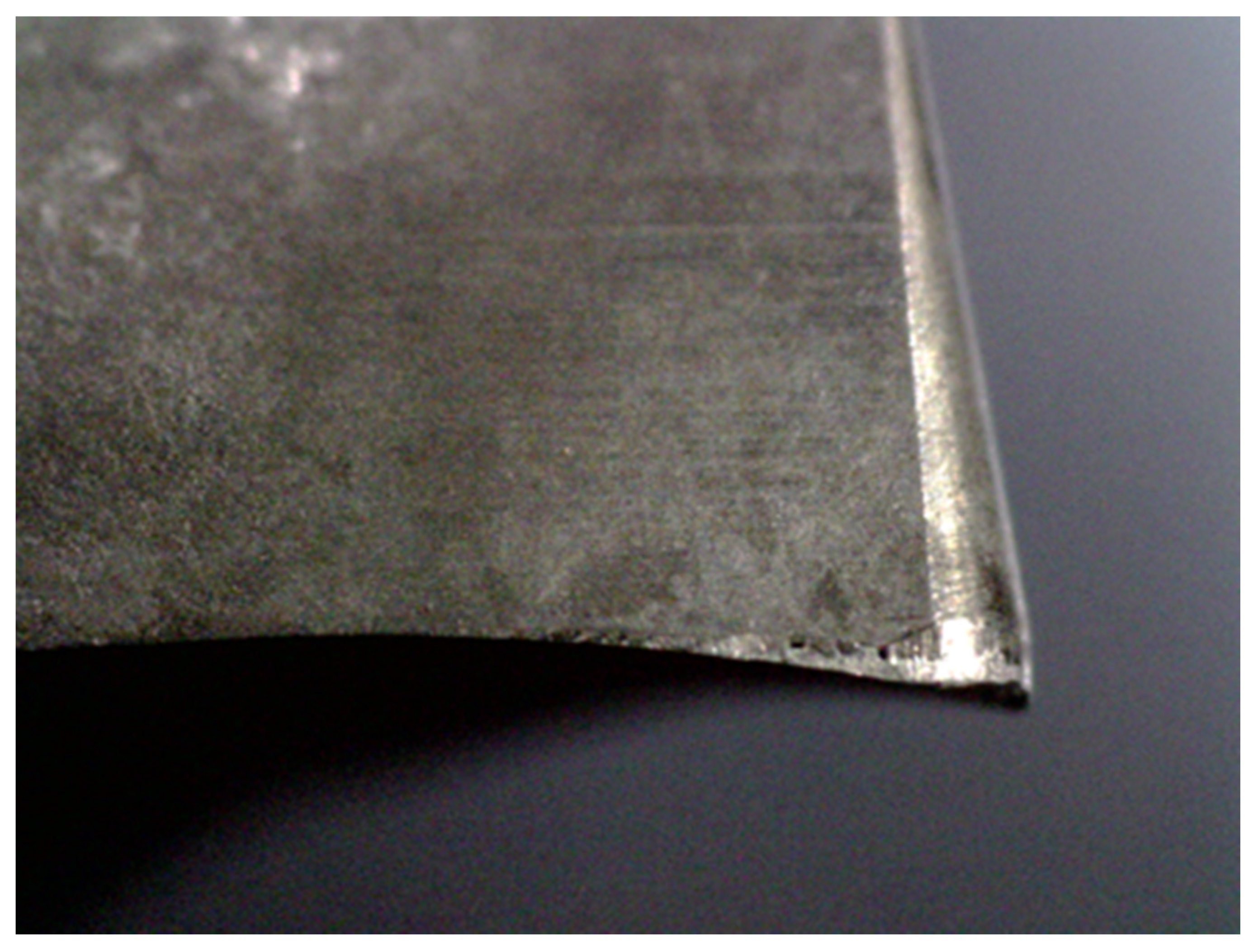
4.1. Experimental Setup

In order to prove the effectiveness of our contribution, the experimental data were measured from a high-speed milling process, which were obtained from the “International PHM Data Challenge Competition in 2010” database [43]. Based on this database, the performance of the proposed method was verified. In the experiment, a high-speed CNC machine (Röders Tech RFM760) with a spindle speed of up to 10,400 rpm was used for the milling operation in the experiment. The experimental structure is shown in Figure 8, and the tool-related parameter information is shown in

Table 1. PHM2010 competition experiment parameter list.

Parameter	Value	Parameter	Value
Machine model	Roders Tech RFM 760	Radial depth of cut	0.125 mm
Workpiece material	Nickel-based superalloy 718	axial cutting depth	0.2 mm
Tool	3-tooth ball nose milling cutter	Number of sensors	3
Spindle speed	10,400 RPM	Number of sensing channels	7
Feed rate	1555 mm/min	Sampling frequency	50 kHz

.

The experimental installation is shown in Figure 9. A Kistler quartz three-component platform dynamometer was mounted between the workpiece and machining table to measure the cutting forces charges. Three Kistler piezo accelerometers were installed on the workpiece to measure the vibration of the workpiece in the X, Y, and Z directions during the milling process. An acoustic emission (AE) sensor was installed on the side of the workpiece to monitor the high-frequency acoustic emission signal during the milling process. The voltage signals were captured by an NI DAQ PCI 1200 board with a 50 kHz frequency. After one horizontal cutting line along the y-axis direction (1st), the cutter then retracted to another starting point with a cutting depth of 0.2 mm in the z-axis (2nd) direction. In each process, the cutter was used to cut the workpiece slope in succession to achieve a complete slope surface. After each processing, a Leica MZ 12 microscope was used to measure the corresponding side surface wear of the cutter. And the proposed approach is coded in MATLAB 2017b, and runs on a server with a 2.40 GHz processor and 64 GB RAM.

4.2. Verification of Method Validity

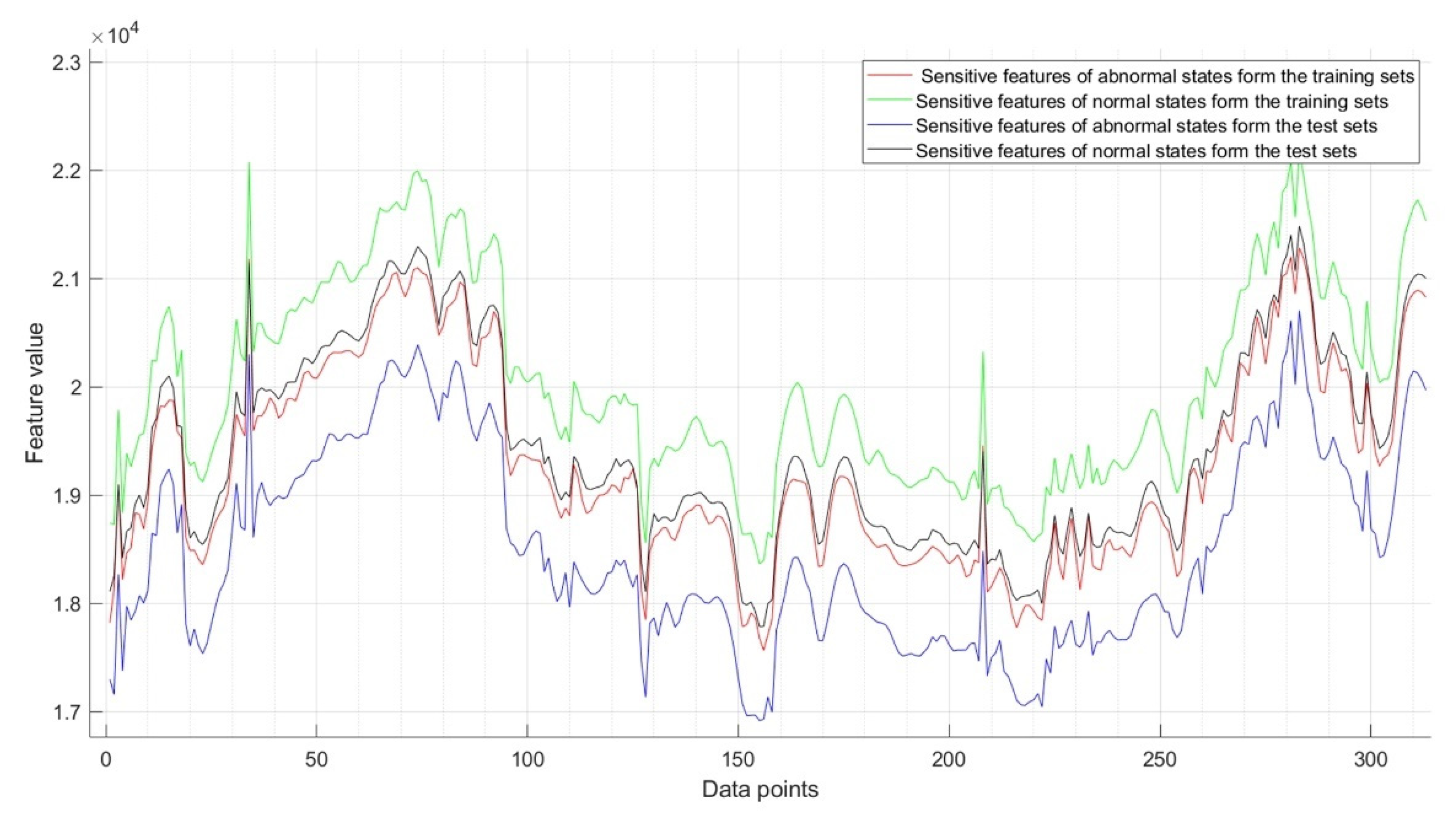
4.2.1. Data Preprocessing and Control Limit Determination

In this paper, the monitoring method of the process was based on point-to-point control limits, but it put forward higher requirements of applicability for the real-time data. The original data contained noise and other irrelevant information, which would interfere with our analysis results, so it was necessary to preprocess the data in the PHM2010 datasets. The wavelet denoising method was used in this research [44]. The denoising effect of the wavelet is related to the wavelet basis function, the threshold selection, and the number of decomposition layers. The sinusoidal signal of the Gaussian white noise with a signal-to-noise ratio of 0.1 was used to test. Part of the test results are shown in Figure 10. After comparing with the original signal, we found that the 5-layer haar wavelet with a heuristic threshold achieved the best results.

Three experimental subsets of the PHM2010 datasets were selected in our research with the record files C1, C4 and C6, and each file contained 315 data samples; the wear values of three edges were collected for each sample. One edge was picked as an example, then the original tool wear values were used to construct the initial control limit, and the existence of random errors was considered to enhance the sample richness (w = w + r). Then, the KDE (described in Section 3.1) was used to obtain the distribution of tool wear. As the purpose of this research was to explain the method, the control limit was set to five levels, which were relatively simple and recorded as (L₁, L₂, L₃, L₄, L₅). The wear state was divided into six types denoted as M₁ to M₆ by the five-level control limit. The final obtained control limit is shown in Figure 11, which was in a pipe shape, and the green area was the first-level control limit range M₁, which indicated that the processing was well controlled. Other colored areas are the different warning control limits ranging from M₂ to M₅, which gave different early warning references as a reminder. If the level control limit was out of tolerance, the M₆ area was reached, which is in an alarm range. At this time, manual inspection can be performed. Of course, more levels of control limits can be set according to actual needs. In Figure 11, the 100th point is divided in more detail to show each level of the control limit. After the multi-level point control limit is completed, the tool state identification process can be implemented.

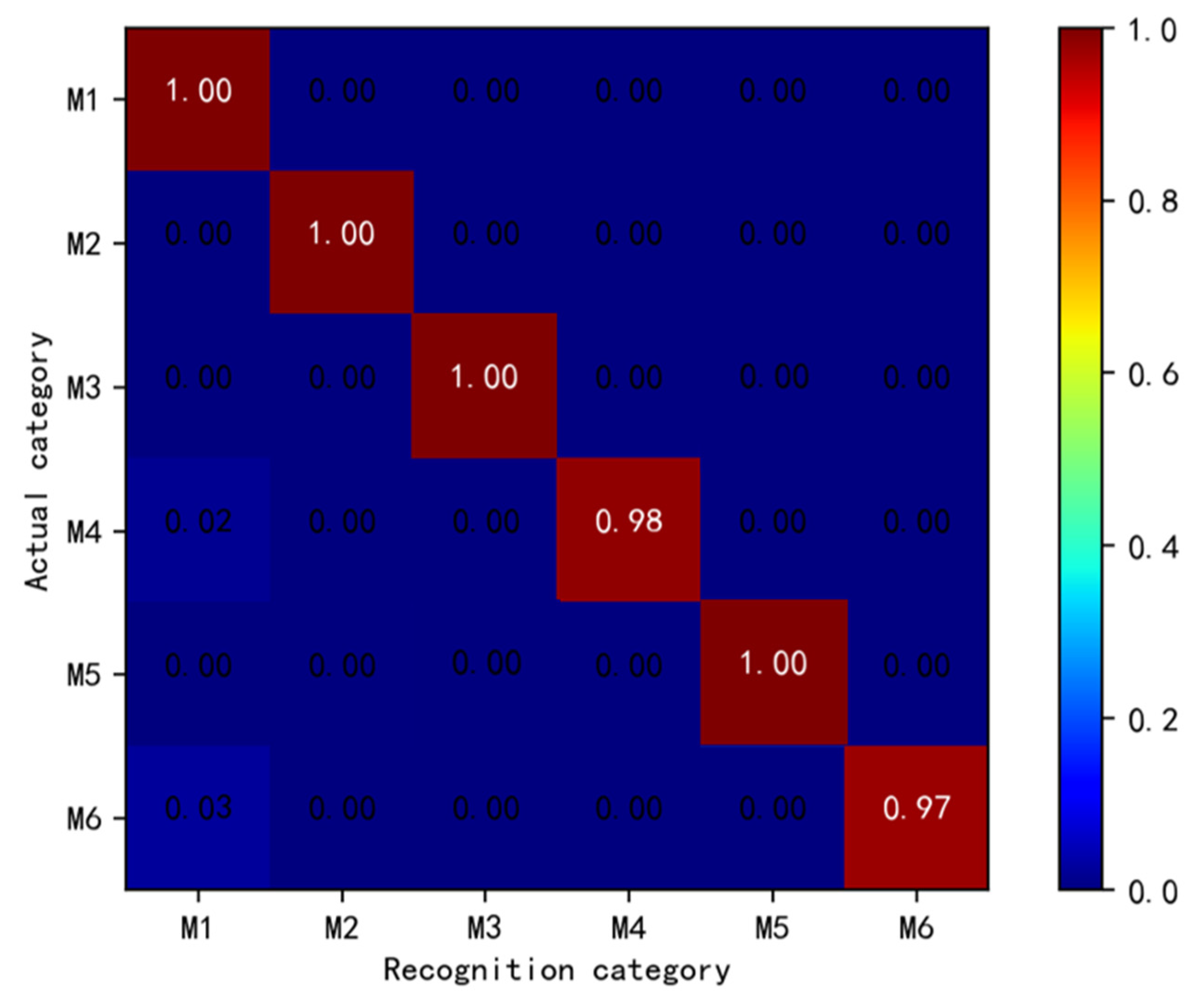
4.2.2. Training and Testing of the CNN Model

For the proposed model, firstly, the data samples of C1 in C1 that belong to the M₁ state were used to confirm the sampling window and to determine the best sampling window (or sensitive window). The result is shown in Figure 12.

The process in Figure 5 was used to obtain the sensitive window size. The test window size was set in a range from 1 to 12,000, and the window sliding step was S = 1. The original signal size was divided into W_i with a sliding step 1, then the CNN algorithm method was used to identify, and the results of the CNN algorithm classification were counted. Since the test sample belonged to M₁, the small window had a better timeliness ability. From Figure 11, it can be found that around 1000–1200 and 2000–2500 had the best recognition accuracy rates, and the window size was appropriate. Considering that the convenience of the subsequent algorithm and small windows had better timeliness than large windows, the optimal window size was selected as 1024.

For the proposed approach, the CNN algorithm was the core part of the entire model. Due to the data size limitation, the larger network would make it easier to over-fit, so when the network becomesf larger and deeper, it would not improve the effect. Additionally, if the number of network layers and the parameters in the layer are different, the number of training samples and the training time required are also different, and its robustness and generalization ability will be affected. In order to obtain the best network structure, the control variable method was adopted in this research; many experiments have also implemented this to determine the number of network layers, convolution kernels, pool size, and activation functions. Finally, the network structure parameters of CNN were designed as shown in

Table 2. The network structure parameters of CNN model.

Network Layer	Key Parameter	Output Shape	Activation Function
Conv1D	Kernel size = 16, stride = 1	1024 × 16	ReLU
Maxpooling1D	Pool size = 2, stride = 1	512 × 16
Conv1D	Kernel size = 32, stride = 1	512 × 32	ReLU
Maxpooling1D	Pool size = 2, stride = 1	256 × 32
Flatten		8192
Dense		6
Softmax			Softmax

.

Then, the subsets of the PHM2010 dataset (which are C1 and C4) were regard as the training set and C6 as the test set to test the recognition ability of the proposed method. The force signal in the X-axis direction was selected for experimentation. The original time series signal was processed by wavelets and we input it into the CNN model. Then, we transformed it into a figure through convolution and pooling for recognition, as shown in Figure 13.

Finally, we conducted statistics and analysis on the results of the CNN recognition. The accuracy and loss rate of the model in the training set C1, C4, and test set C6 are shown in Figure 14, respectively. It can be seen from Figure 14 that, as the number of trainings increased, the accuracy of the training set and the test set continued to increase, and the loss value continued to decrease.

Then, the recognition effect was given in the form of a confusion matrix, which is shown in Figure 15. It can be seen from Figure 15 that the model had good recognition performance in both the training set and test set. Due to less grading of control limits, the comprehensive recognition accuracy of the model was very high. This shows that there was no problem for the proposed model in identifying more types, and there was space for distinguishing more sates under multi-level control limits. In addition, the average response time of the model was 0.0661 s. These results reflect good monitoring performance of the model.

In addition, other classification algorithms were used in this research, such as the support vector machine (SVM), ANN, K-Nearest Neighbor (KNN), and Decision Tree (Tree), to compare with the CNN as recognizers in the proposed approach. For SVM, the parameters that need to be adjusted mainly include the penalty coefficient C and the kernel function coefficient G. In this research, the feature dimension is much lower than the sample size, so this research uses Gaussian kernel function. The grid search method is used to perform the global optimization of SVM parameters and to specify the value range of C and G, at the same time, specify the parameter step size and then arrange and combine the possible values of C and G to generate the parameter “net of C and G″. grid”. Then select a combination of C and G parameters for SVM training each time, and use cross-validation to evaluate the performance of the model, traverse all parameter combinations, and select the optimal parameter combination of C and G with the average recognition accuracy as the evaluation index. Through grid search, among the hyperparameters, C = 10 and G = 0.1 have the highest scores. This is our final parameter candidate. For ANN, first use PCA for dimensionality reduction, and then start with a smaller value. If under-fitting, then slowly add more layers and neurons, if over-fitting, reduce the number of layers and neurons. At the same time, batch normalization, dropout, and regularization are introduced to reduce overfitting. Finally, the number of layers is set to 3, the number of inputs is 3, the number of hidden neurons is 12, and the output category is 6. The selection of parameters in KNN is also determined by the grid search method. The final nearest neighbor value K is set to 7, the distance metric is set to Manhattan distance, and the decision rule is set to the majority voting method. For decision trees, the Gini coefficient is used to evaluate impurity, and the random method is set to find the best segmentation node.

The comprehensive performance results of each algorithm can be obtained and shown in

Table 3. The test results of multiple classification algorithms for comparison.

Recognizer	Recognition Accuracy	Average Response Time
CNN	97.2%	0.0661 s
SVM	96.5%	0.0382 s
ANN	95.1%	0.0748 s
KNN	94.7%	0.0537 s
Tree	95.3%	0.0279 s

. The corresponding response time is recorded by the tic/toc time counter in MATLAB. It can be seen from Table 3 that KNN is taking more time than the SVM, which is not usually the case. We guess that the potential reasons mainly include two points, one is that the number of samples and feature dimensions may have different effects on the two algorithms. Second is that the SVM only needs to determine the side of the boundary for new observation data, but each observation data must be compared with other data items for KNN, which will produce a huge calculation cost. Furthermore, it can be seen from Table 3 that the CNN recognizer had the highest recognition accuracy. Although the average response time was slightly longer than other recognizers, it was completely sufficient for practical applications.

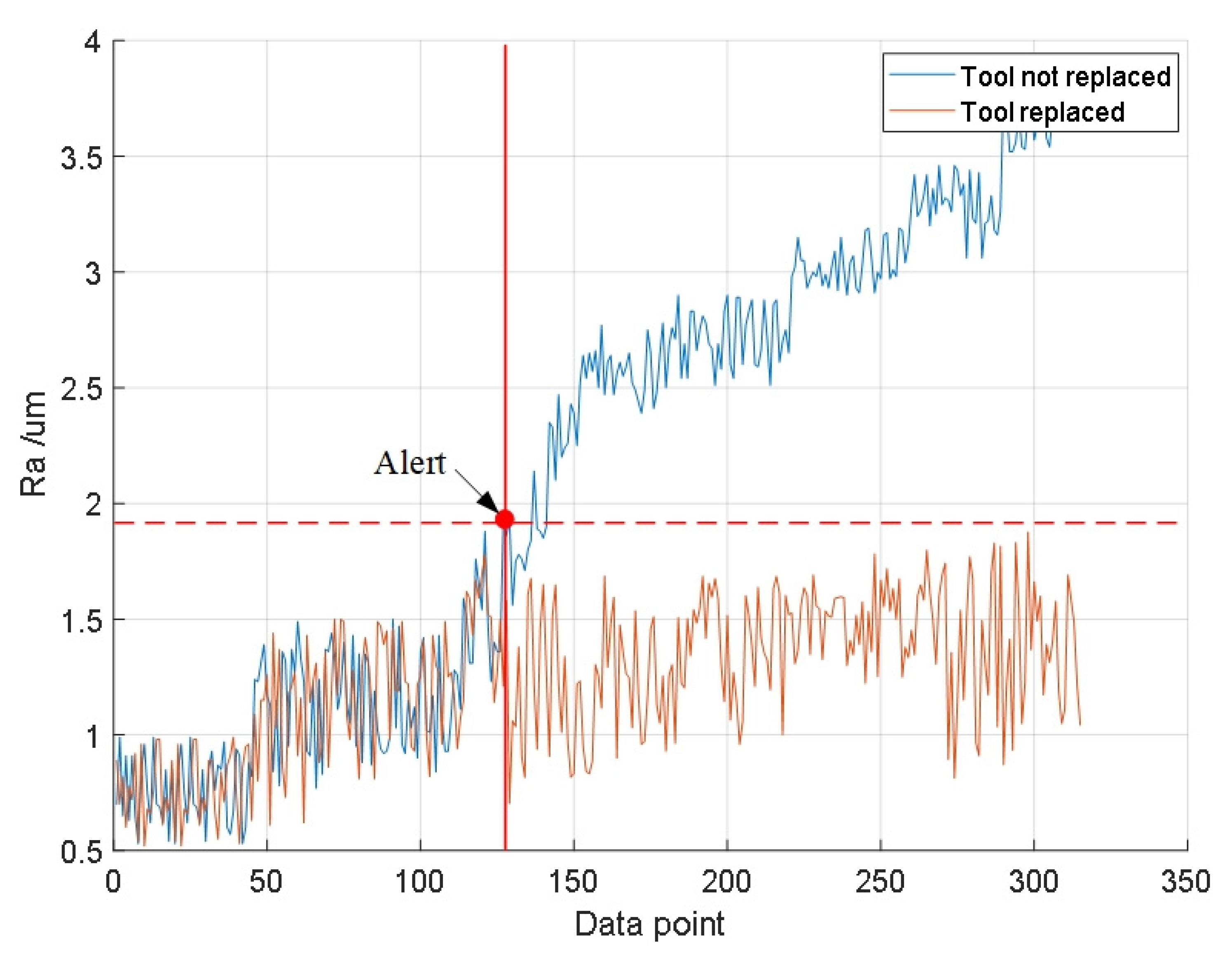
4.3. Actual Case Verification

In order to further verify the effectiveness of the method under multiple operating conditions, we carried out actual tool wear tests to verify. There are a lot of data that can be obtained in the machine tool system. This test considers that the tool wear is relatively related to the cutting force signal, so the cutting force is used to monitor the tool wear states. During the cutting process, the feed rate is set to 2000 mm/min. The cutting depth is 1 mm, and the data sampling frequency is 50 KHz. A square workpiece with a side length of 10 cm is cut. In this experiment, the surface roughness average value R_a is used to characterize the processing quality of the workpiece. After the cutting is completed, the roughness of the cut surface is measured, and the average of each surface is measured four times. At the same time, in order to describe the wear degradation process of the tool, the tool wear is measured with a Dino-Lite microscope each time. The processing environment as well as the measurement of surface roughness and tool wear is shown in Figure 16. The spindle speed is respectively 4000 r/min, 6000 r/min, 8000 r/min, and 20 data sets are collected under each group of different working conditions. As the tool wears, the cutting quality will continue to deteriorate. Two operating strategies are set in this experiment. Under each working condition, 10 sets of tools are not replaced after reach M₅, and the remaining ten sets are detected as M₅ with new tool to cut the workpiece.

Use the same method described in Section 3 to establish the control limits under 4000 r/min, 6000 r/min, and 8000 r/min. For each working condition, the data sets were divided into the training set and the test set with the ratio of 7:3, and then perform the algorithm training and testing. The results are shown in

Table 4. The performance of condition monitoring model under different working conditions.

Test Conditions	Recognition Accuracy of Training Sets	Recognition Accuracy of Training Sets
4000 r/min	100%	99.5%
6000 r/min	99.9%	99.5%
8000 r/min	99.9%	99.6%

. Comparing the recognition effect under the three working conditions, it can be found that the obtained results show that the recognition effect is not affected by the working conditions.

After measuring the surface roughness of the workpiece and the current tool wear, it is found that the tool has been obviously worn after the proposed method is used to identify the tool state to M₅, as shown in Figure 17. Then the roughness measuring instrument is used to check the surface roughness of the workpiece, as shown in Figure 18, it can be found that the tool wear at this time caused the increase of the surface roughness of the workpiece. Taking the identification M₅ as the alert point, it can be seen form Figure 18 that the surface roughness after the alert point basically exceeds 2 μm, which is quite different from before the alert point. At the same time, comparing with another set of experiments, comparing the different trend of roughness after the tool is not changed and the tool is replaced with new tool after being identified as M₅, it can be found that the proposed method monitors the tool wear to ensure that the tool is in good states under different working conditions. The proposed approach can effectively improve the processing quality.

5. Discussion

One of the major innovations and advantages of the proposed approach is that the criteria for judging abnormal conditions based on the control limit method are extended. The original Shewhart control limit mainly analyzes one sampling point, while the entire process is considered for the point-related control limit established in the proposed approach, which expands the scope of application of control limits. For example, one of the judgment standards for the traditional control limit is to judge the next state trend based on the state of several consecutive points, which is shown in Figure 19 (a → b → c). As the point-related control limit is considered according to the entire process, it can establish a state transition path (K₁ → K₂ → K₃), which can reflect more comprehensive information. It can even use the transition relationship from the difference path to infer the specific cause for abnormality when the sample is sufficient.

In addition, another advantage for the proposed approach is that the condition monitoring model solved the influence of feature selection and feature extraction, which can influence the stability of the recognition stability. After the data are extracted into different features, the information it contains is incomplete, and the sensitive features obtained by correlation analysis are easily changed, as shown in Figure 20. Therefore, the method of inputting different features and performing state monitoring can easily lead to misidentification, which will affect the performance of the model stability. The proposed approach is an end-to-end identification method, and the input is direct raw data, which avoids this problem.

6. Conclusions

To solve the problem of tool wear state monitoring for aerospace manufacturing processes, we have proposed a tool condition monitoring method based on a Convolutional Neural Network (CNN). Firstly, the tool wear level was divided into different state modes according to the probability density interval based on the kernel density estimation (KDE). The corresponding state modes were connected to obtain the point-to-point control limit. Then, a state recognition model based on a CNN was developed, and the sensitivity of the monitoring window was considered in the model. Finally, the PHM2010 dataset and actual case were used for feasibility verification of the proposed method. The experimental results proved the applicability of the proposed method for tool state monitoring. Compared with the traditional condition monitoring method, the idea of statistical process control was combined in the model to construct a multi-level point-to-point control limit, and, as in the discussion, the criteria for judging abnormal conditions were extended compared with the traditional SPC. In addition, the influence of feature-to-recognition stability was overcome by the proposed model, whereas the traditional data-based condition monitoring methods rely heavily on the selection of appropriate sensitive features. Of course, the currently proposed approach still has certain limitations, as different models need to be trained to achieve better monitoring results for different working conditions, but this problem is also unavoidable in data-driven methods. To solve this problem, it is necessary to conduct further research on the proposed model. However, the proposed method already can effectively monitor the tools’ condition, and when the status of the tool is recognized, the different corresponding measures (such as tool failure or tool replacement) can be taken according to different recognition states to always keep the tool in the best condition and reduce defective parts.

The proposed method can effectively monitor tool wear states under specific working conditions, and according to data verification, the method proposed in this paper has a higher recognition accuracy. Compared with other industries, aerospace has higher requirements for the accuracy of parts. The proposed method can more effectively meet the manufacturing needs of the aerospace field. As shown in the case, the surface roughness of parts can be effectively controlled by monitoring tools condition through proposed method. Therefore, the proposed method is of great value for ensuring the manufacturing quality of aerospace parts during the production process.

References

1. Liu, Z.; Zhang, L. A review of failure modes, condition monitoring and fault diagnosis methods for large-scale wind turbine bearings. Measurement 2020, 149, 107002. [Google Scholar] [CrossRef]
2. Trzun, Z.; Vrdoljak, M.; Cajner, H. The Effect of Manufacturing Quality on Rocket Precision. Aerospace 2021, 8, 160. [Google Scholar] [CrossRef]
3. Djebko, K.; Puppe, F.; Kayal, H. Model-Based Fault Detection and Diagnosis for Spacecraft with an Application for the SONATE Triple Cube Nano-Satellite. Aerospace 2019, 6, 105. [Google Scholar] [CrossRef] [Green Version]
4. Hong, W.; Cai, W.; Wang, S.; Tomovic, M.M. Mechanical wear debris feature, detection, and diagnosis: A review. Chin. J. Aeronaut. 2018, 31, 867–882. [Google Scholar] [CrossRef]
5. Javed, K.; Gouriveau, R.; Li, X.; Zerhouni, N. Tool wear monitoring and prognostics challenges: A comparison of connectionist methods toward an adaptive ensemble model. J. Intell. Manuf. 2018, 29, 1873–1890. [Google Scholar] [CrossRef]
6. Bhuiyan, M.S.H.; Choudhury, I.A.; Dahari, M. Monitoring the tool wear, surface roughness and chip formation occurrences using multiple sensors in turning. J. Manuf. Syst. 2014, 33, 476–487. [Google Scholar] [CrossRef]
7. Liu, Y.; Hong, S.; Zio, E.; Liu, J. Fault Diagnosis and Reconfigurable Control for Commercial Aircraft with Multiple Faults and Actuator Saturation. Aerospace 2021, 8, 108. [Google Scholar] [CrossRef]
8. Valtierra-Rodriguez, M.; Amezquita-Sanchez, J.; Garcia-Perez, A.; Camarena-Martinez, D. Complete Ensemble Empirical Mode Decomposition on FPGA for Condition Monitoring of Broken Bars in Induction Motors. Mathematics 2019, 7, 783. [Google Scholar] [CrossRef] [Green Version]
9. Oo, H.; Wang, W.; Liu, Z. Tool wear monitoring system in belt grinding based on image-processing techniques. Int. J. Adv. Manuf. Technol. 2020, 111, 2215–2229. [Google Scholar] [CrossRef]
10. Basora, L.; Bry, P.; Olive, X.; Freeman, F. Aircraft Fleet Health Monitoring with Anomaly Detection Techniques. Aerospace 2021, 8, 103. [Google Scholar] [CrossRef]
11. Goodall, P.; Pantazis, D.; West, A. A cyber physical system for tool condition monitoring using electrical power and a mechanistic model. Comput. Ind. 2020, 118, 103223. [Google Scholar] [CrossRef]
12. Basora, L.; Olive, X.; Dubot, T. Recent Advances in Anomaly Detection Methods Applied to Aviation. Aerospace 2019, 6, 117. [Google Scholar] [CrossRef] [Green Version]
13. Qin, A.; Guo, L.; You, Z.; Gao, H.; Wu, X.; Xiang, S. Research on automatic monitoring method of face milling cutter wear based on dynamic image sequence. Int. J. Adv. Manuf. Technol. 2020, 110, 3365–3376. [Google Scholar] [CrossRef]
14. Fernández-Robles, L.; Sánchez-González, L.; Díez-González, J.; Castejón-Limas, M.; Pérez, H. Use of image processing to monitor tool wear in micro milling. Neurocomputing 2020, 452, 333–340. [Google Scholar] [CrossRef]
15. Doğru, A.; Bouarfa, S.; Arizar, R.; Aydoğan, R. Using Convolutional Neural Networks to Automate Aircraft Maintenance Visual Inspection. Aerospace 2020, 7, 171. [Google Scholar] [CrossRef]
16. Lamraoui, M.; Thomas, M.; El Badaoui, M. Cyclostationarity approach for monitoring chatter and tool wear in high speed milling. Mech. Syst. Signal. Process. 2014, 44, 177–198. [Google Scholar] [CrossRef]
17. Mohanraj, T.; Shankar, S.; Rajasekar, R.; Sakthivel, N.R.; Pramanik, A. Tool condition monitoring techniques in milling process—A review. J. Mater. Res. Technol. 2020, 9, 1032–1042. [Google Scholar] [CrossRef]
18. Rizal, M.; Ghani, J.A.; Nuawi, M.Z.; Haron, C.H.C. Cutting tool wear classification and detection using multi-sensor signals and Mahalanobis-Taguchi System. Wear 2017, 376–377, 1759–1765. [Google Scholar] [CrossRef]
19. Brito, L.C.; Susto, G.A.; Brito, J.N.; Duarte, M.A.V. An explainable artificial intelligence approach for unsupervised fault detection and diagnosis in rotating machinery. Mech. Syst. Signal. Process. 2022, 163, 108105. [Google Scholar] [CrossRef]
20. Aykroyd, R.G.; Leiva, V.; Ruggeri, F. Recent developments of control charts, identification of big data sources and future trends of current research. Technol. Forecast. Soc. Chang. 2019, 144, 221–232. [Google Scholar] [CrossRef]
21. Fuqua, D.; Razzaghi, T. A cost-sensitive convolution neural network learning for control chart pattern recognition. Expert Syst. Appl. 2020, 150, 113275. [Google Scholar] [CrossRef]
22. Lin, C.; Lu, M.; Yang, S.; Lee, M. A Bayesian Control Chart for Monitoring Process Variance. Appl. Sci. 2021, 11, 2729. [Google Scholar] [CrossRef]
23. Aziz Kalteh, A.; Babouei, S. Control chart patterns recognition using ANFIS with new training algorithm and intelligent utilization of shape and statistical features. ISA Trans. 2020, 102, 12–22. [Google Scholar] [CrossRef]
24. Vapnik, V.N. An overview of statistical learning theory. IEEE Trans. Neural. Netw. 1999, 10, 988–999. [Google Scholar] [CrossRef] [Green Version]
25. Yu, M.; Wu, C.; Wang, Z.; Tsung, F. A robust CUSUM scheme with a weighted likelihood ratio to monitor an overdispersed counting process. Comput. Ind. Eng. 2018, 126, 165–174. [Google Scholar] [CrossRef]
26. Lee, T.; Baek, C. Block wild bootstrap-based CUSUM tests robust to high persistence and misspecification. Comput. Stat. Data Anal. 2020, 150, 106996. [Google Scholar] [CrossRef]
27. Mukherjee, A.; Chong, Z.L.; Khoo, M.B.C. Comparisons of some distribution-free CUSUM and EWMA schemes and their applications in monitoring impurity in mining process flotation. Comput. Ind. Eng. 2019, 137, 106059. [Google Scholar] [CrossRef]
28. Dao, P.B. A CUSUM-Based Approach for Condition Monitoring and Fault Diagnosis of Wind Turbines. Energies 2021, 14, 3236. [Google Scholar] [CrossRef]
29. Ajadi, J.O.; Zwetsloot, I.M.; Tsui, K. A New Robust Multivariate EWMA Dispersion Control Chart for Individual Observations. Mathematics 2021, 9, 1038. [Google Scholar] [CrossRef]
30. Ding, S.; Li, X.; Dong, X.; Yang, W. The Consistency of the CUSUM-Type Estimator of the Change-Point and Its Application. Mathematics 2020, 8, 2113. [Google Scholar] [CrossRef]
31. Soualhi, M.; Nguyen, K.T.P.; Medjaher, K. Pattern recognition method of fault diagnostics based on a new health indicator for smart manufacturing. Mech. Syst. Signal. Process. 2020, 142, 106680. [Google Scholar] [CrossRef]
32. Nesci, A.; De Martin, A.; Jacazio, G.; Sorli, M. Detection and Prognosis of Propagating Faults in Flight Control Actuators for Helicopters. Aerospace 2020, 7, 20. [Google Scholar] [CrossRef] [Green Version]
33. Kim, T.; Cho, S. Optimizing CNN-LSTM neural networks with PSO for anomalous query access control. Neurocomputing 2021, 456, 666–677. [Google Scholar] [CrossRef]
34. Mashuri, M.; Ahsan, M.; Lee, M.H.; Prastyo, D.D. PCA-based Hotelling’s T2 chart with fast minimum covariance determinant (FMCD) estimator and kernel density estimation (KDE) for network intrusion detection. Comput. Ind. Eng. 2021, 158, 107447. [Google Scholar] [CrossRef]
35. Tian, Q.; Wang, H. Predicting Remaining Useful Life of Rolling Bearings Based on Reliable Degradation Indicator and Temporal Convolution Network with the Quantile Regression. Appl. Sci. 2021, 11, 4773. [Google Scholar] [CrossRef]
36. Chen, H.; Xu, K.; Chen, L.; Jiang, Q. Self-Expressive Kernel Subspace Clustering Algorithm for Categorical Data with Embedded Feature Selection. Mathematics 2021, 9, 1680. [Google Scholar] [CrossRef]
37. Dai, J.; Liu, Y.; Chen, J. Feature selection via max-independent ratio and min-redundant ratio based on adaptive weighted kernel density estimation. Inf. Sci. 2021, 568, 86–112. [Google Scholar] [CrossRef]
38. Shao, R.; Hu, W.; Wang, Y.; Qi, X. The fault feature extraction and classification of gear using principal component analysis and kernel principal component analysis based on the wavelet packet transform. Measurement 2014, 54, 118–132. [Google Scholar] [CrossRef]
39. Hou, L.; Qu, H. Automatic recognition system of pointer meters based on lightweight CNN and WSNs with on-sensor image processing. Measurement 2021, 183, 109819. [Google Scholar] [CrossRef]
40. Phisannupawong, T.; Kamsing, P.; Torteeka, P.; Channumsin, S.; Sawangwit, U.; Hematulin, W.; Jarawan, T.; Somjit, T.; Yooyen, S.; Delahaye, D.; et al. Vision-Based Spacecraft Pose Estimation via a Deep Convolutional Neural Network for Noncooperative Docking Operations. Aerospace 2020, 7, 126. [Google Scholar] [CrossRef]
41. Lu, Z.; Wang, M.; Dai, W. A condition monitoring approach for machining process based on control chart pattern recognition with dynamically-sized observation windows. Comput. Ind. Eng. 2020, 142, 106360. [Google Scholar] [CrossRef]
42. Long, Y.; Zhou, W.; Luo, Y. A fault diagnosis method based on one-dimensional data enhancement and convolutional neural network. Measurement 2021, 180, 109532. [Google Scholar] [CrossRef]
43. PHM Society. PHM Data Challenge. 2010. Available online: https://www.Phmsociety.org/competition/phm/10S (accessed on 8 October 2021).
44. Yan, R.; Gao, R.X.; Chen, X. Wavelets for fault diagnosis of rotary machines: A review with applications. Signal Process. 2014, 96, 1–15. [Google Scholar] [CrossRef]
Figure 1. The algorithm structure diagram of Convolutional Neural Network (CNN). Input signal D1, followed by convolution and pooling, and then outputs N can be obtained from the fully connected layer.
Aerospace 08 00335 g001
Figure 2. The research framework of the state monitoring approach.
Aerospace 08 00335 g002
Figure 3. The multi-level point-to-point control limit.
Aerospace 08 00335 g003
Figure 4. The method of setting control limits based on KDE.
Aerospace 08 00335 g004
Figure 5. The process of optimal sampling window determination.
Aerospace 08 00335 g005
Figure 6. The state recognition process based on moving sliding window.
Aerospace 08 00335 g006
Figure 7. The structure of the 1D-CNN.
Aerospace 08 00335 g007
Figure 8. The experimental structure of the 2010 International PHM Data Challenge Competition.
Aerospace 08 00335 g008
Figure 9. The schematic diagram of sensor pasting and processing during data acquisition.
Aerospace 08 00335 g009
Figure 10. Part of the results of wavelet denoising for Gaussian white noise.
Aerospace 08 00335 g010
Figure 11. The multi-level point-to-point control limit for PHM2010 datasets.
Aerospace 08 00335 g011
Figure 12. The sensitive window size determination schematic.
Aerospace 08 00335 g012
Figure 13. The graph structure obtained from the original time series data after pooling layer.
Aerospace 08 00335 g013
Figure 14. The changes of accuracy and loss form the training set and test set in the CNN model. (a) The changes of accuracy in CNN model; (b) The changes of loss in CNN model.
Aerospace 08 00335 g014
Figure 15. The result of the confusion matrix for model recognition.
Aerospace 08 00335 g015
Figure 16. Schematic diagram of test environment and measurement of surface roughness and tool wear.
Aerospace 08 00335 g016
Figure 17. Tool wear state at M5.
Aerospace 08 00335 g017
Figure 18. The influence of the tool on the surface roughness of the workpiece.
Aerospace 08 00335 g018
Figure 19. The difference between the two methods for abnormal judgment. (a) The abnormal judgment for traditional control limits; (b) The abnormal judgment for proposed control limits.
Aerospace 08 00335 g019
Figure 20. The change in features for a data-based method.
Aerospace 08 00335 g020