Article

Blade Roughness Effects on Compressor and Engine Performance—A CFD and Thermodynamic Study

by
Jasem Alqallaf
1,2,* and
Joao A. Teixeira
1
1
School of Aerospace, Transport and Manufacturing, Cranfield University, Cranfield, Bedford MK43 0AL, UK
2
Kuwait Army, Kuwait Ministry of Defense, Safat 13128, Kuwait
*
Author to whom correspondence should be addressed.
Aerospace 2021, 8(11), 330; https://doi.org/10.3390/aerospace8110330
Submission received: 19 September 2021 / Revised: 31 October 2021 / Accepted: 1 November 2021 / Published: 4 November 2021
(This article belongs to the Section Aeronautics)

Abstract

:
Degradation of compressors is a common concern for operators of gas turbine engines (GTEs). Surface roughness, due to erosion or fouling, is considered one of the major factors of the degradation phenomenon in compressors that can negatively affect the designed pressure rise, efficiency, and, therefore, the engine aero/thermodynamic performance. The understanding of the aerodynamic implications of varying the blade surface roughness plays a significant role in establishing the magnitude of performance degradation. The present work investigates the implications due to the degradation of the compressor caused by the operation in eroding environments on the gas turbine cycle performance linking, thereby, the compressor aerodynamics with a thermodynamic cycle. At the core of the present study is the numerical assessment of the effect of surface roughness on compressor performance employing the Computational Fluid Dynamics (CFD) tools. The research engine test case employed in the study comprised a fan, bypass, and two stages of the low pressure compressor (booster). Three operating conditions on the 100% speed-line, including the design point, were investigated. Five roughness cases, in addition to the smooth case, with equivalent sand-grain roughness ( k s ) of 15, 30, 45, 60, and 150 µm were simulated. Turbomatch the Cranfield in-house gas turbine performance simulation software, was employed to model the degraded engine performance. The study showed that the increase in the uniform roughness is associated with sizable drops in efficiency, booster pressure ratio (PR), non-dimensional mass flow (NDMF), and overall engine pressure ratio (EPR) together with rises in turbine entry temperature (TET) and specific fuel consumption (SFC). The performance degradation evaluation employed variables such as isentropic efficiency ( η i s ), low pressure compressor (LPC) PR, NDMF, TET, SFC, andEPR. The variation in these quantities showed, for the maximum blade surface degradation case, drops of 7.68%, 2.62% and 3.53%, rises of 1.14% and 0.69%, and a drop of 0.86%, respectively.

1. Introduction

The increasing demand for energy around the world is accompanied by growing concerns about energy security. Performance criteria for machinery and its operation are becoming ever more meticulously defined and components are pushed ever closer to their limits [1]. Gas turbine engines (GTEs) play an important role in the global economy and there has been a continuous increase in their numbers since their introduction [2]. The superior power density and operational efficiency of GTEs made them widespread in the propulsion of aircraft and ships, and in the power generation industry [3,4]. However, there are a number of issues relating to the life cycle management of GTEs, including reliability, operational and maintenance costs, and the availability of substitute components [5].
The performance of GTEs operating over extended periods is subject to deterioration, impairing their efficiency and power output. This is due to a number of causes, mostly erosion and fouling [6], and the continuous requirement for maintenance to sustain high level of performance. Unlike for power generation, gas turbines used for aircraft propulsion are not fitted with elaborate intake filters. Therefore, they are exposed to solid particle erosion (SPE) causing excessive wear, fouling, and corrosion resulting in the permanent deformation of blade surfaces and increasing the surface roughness or even failure [7,8]. The problem is exacerbated for GTEs which are used in arid environments such as the Middle East, where any deterioration on the surface would result in changes in the blade’s aerodynamics and wettability behaviours [9,10,11]. Furthermore, the compression system, including the fan and the compressor, are the most critical components in GTEs as, while they contribute to the overall cycle efficiency, they dictate the operability range demanding aerodynamics and aeromechanics design efforts [12,13]. Compressor blades are highly sensitive to boundary layer separation as well as to the operation with added blockage due to increased surface roughness [14]. Moreover, the rise in total pressure in compressors results in adverse pressure gradients and, thus, is characterized by unstable boundary layers that significantly contribute to losses [15]. Along with blade geometry alterations, a deteriorated compressor can exhibit complex surface roughness patterns [16]. Blade surface abrasion can then lead to a reduced engine mass flow ( m ˙ ) due to increased blockage effects and, hence, to a reduction in pressure ratio (PR) and efficiency. These, in turn, reduce the efficiency of the coupling mechanisms linking compressor and turbine, with a consequent loss of efficiency and output power that can range from 2% to as much as 15–20% when blade surfaces are heavily deteriorated [17]. Furthermore, the aerodynamic performance of GTEs is particularly sensitive to changes in the low pressure compressors (LPC) [18,19]. According to the literature, the LPC blade surface roughness is the reason for between 70% and 85% of the total losses in performance during the continuous operation of GTEs [17].
An extensive review of research into the deterioration of turbomachines was provided by Hamed et al. [20]. The authors concluded that compressor blading deterioration was a major cause of loss in performance. They found that alterations in compressor airfoil geometry caused by erosion, including reduction in blade chord, increase in tip clearance, increase in surface roughness, and increase in trailing edge (TE) sharpness, cause degradation of the cycle performance. Several investigators have studied how tip clearance size, alterations in the shape of the compressor blades, and increased blade surface roughness affect GTE performance. Bammert and Woelk [21], investigated the effects of blade surface roughness on an axial compressor experimentally. They found that with a roughness of equivalent sand-grain roughness (ks) = 180 µm the static pressure ratio reduced by up to 30%, the volume flow rate decreased by 15–20%, and the m ˙ between 6 and 13%. A numerical study by Zhihui and Yanming [22] examined how wall roughness affects the performance of an axial compressor. The roughness values of the shroud hub and blade were ks = 5, 20, and 40 µm, respectively. The two key results were: (1) The loss in peak efficiency of the compressor was almost entirely (95.3%) due to the roughness of the blade, only 3.6% being due to roughness of the surface of the hub and 1.1% due to the roughness of the casing surface; (2) When the GTE operated at its design point (DP), increased roughness of the compressor blades stimulated the growth of a boundary layer with average thickness near the hub surface increasing less than that near the shroud surface. This added to the strong interaction between the boundary layer at the end wall and leakage flow. Compared to a “smooth” compressor, added roughness also increased tip leakage, particularly in the presence of a rough shroud surface and circumferential blockage near the shock wave region. El-Sayed [23], demonstrated experimentally the effects of increasing the surface roughness on a compressor blade and its performance by ingesting 2.5 kg of sand into a high speed axial flow compressor. This author mentions that operating a GTE for 6000 to 8000 h was found to be enough to cause severe erosion of the blade leading edge (LE) and pressure side (PS) and, thus, lead to an increase in surface roughness as a result. Changes in pressure distribution around the blade were observed which caused an earlier laminar to turbulent transition in the boundary layer. An increase in blade tip leakage and LE erosion was found be responsible for a 4% drop in efficiency. The suction side (SS) was, however, largely unaffected in most of the experiments. Further observations included a 3.5% drop in the stage loading coefficient. Generally, the provision of roughness, as demonstrated by the function of dimples in golf balls, is known to affect laminar to turbulent transition in boundary layers and, hence, impact the drag budget of aerodynamic shapes. This explains that, while most authors agree that the increase in blade roughness is associated with an increment in profile losses together with other aerodynamic penalties, it can nevertheless, under specific circumstances, lead to an actual performance improvement as reported below. Wang et al. [24] demonstrated that the efficiency and stability of compressors are notably affected by increasing the blades surface roughness. The researchers clarified that for a low Reynolds number ( R e     10 5 ), the onset of the boundary layer transition on the compressor blade surface is delayed and the laminar flow tends to separate, which forms a separated shear layer that undergoes a subsequent transition to turbulent flow. This is denoted as the separation flow transition and a Laminar Separation Bubble, LSB, will be visible on the blade surface. With a further decrease in R e , the compressor blade loss will increase rapidly on account of the growth of the LSB, especially when R e decreases below a critical value where there is a risk of severe laminar separation without turbulent reattachment. Furthermore, they examined how the blade’s performance was influenced for different values of surface roughness. The study carried out and investigated numerically the impact of roughness in the range ks = 322.4 to 3255 µm, at four locations on the SS of a compressor blade at R e = 1.5 × 10 5 . The paper presents no correlation between the particular ks values employed in the study and experimentally observed GTE component roughness. The major findings were: (1) Maximum achieved reductions in profile loss were 14.6, 16.0, 16.5, and 10.2% with surface roughness, ks = 973.4 µm, at the four locations, respectively; (2) The roughness of the LE was the main factor in eradicating laminar separation and advancing aerodynamic performance. At ks = 973.4 µm, a roughened surface extending from the LE, covering 10% of the SS was sufficient to eliminate a laminar separation bubble decreasing the profile loss by 14.6%. Increasing the roughened area to half of the SS produced little additional profile loss. For a much larger value of surface roughness of ks = 3267.4 µm, the development of a boundary layer, and aerodynamic performance were more responsive to the area that had been roughened. With ks = 3267.4 µm, there was an apparent decrease in profile loss of up to 30% of the roughened SS. Back et al. [25] examined experimentally the effects of roughness on the aerodynamic behaviour of a low-speed linear compressor cascade. Surface roughness of ks = 180, 300, 425, and 850 µm were utilised, which, according to the authors, are common values found on compressor blades in operational GTEs. It is worth noting that these researchers justified the ks values employed in the study as being due to contributions such as dust, sand, and salt, which in industrial compressors can combine with water, oil and moisture to modify the blade profile and roughen the surface. The following results were reported: (1) With an increase in the roughness of the surface of the compressor blade, the axial velocity decreased and pressure loss grew; (2) For the four given roughness values, the corresponding decreases in axial velocity ratio were 0.1, 2.1, 2.5, and 5.4%, respectively; (3) Pressure loss increased by 12, 44, 132, and 217%, respectively; (4) Deviation, axial velocity, and pressure loss were the most sensitive parameters to surface roughness. Sun et al. [26], developed a numerical model to examine the effect of roughness on compressor performance using test values of ks = 2.11, 2.72, 16.24, 25.53, and 27.41 µm at four operating conditions. The results show that the drop in compressor flow rate, caused by increasing surface roughness conditions, ranged from 0.36% at the lowest ks value to 2.01% for the highest ks at the 100% speed-line. The greater the surface roughness of the compressor blade, the greater the adverse effects on efficiency, power, m ˙ , and PR.
This paper employs an in-house LPC compressor model inspired by NASA’s E3 engine [27,28,29]. The research focuses on the performance degradation brought about by the increase in roughness of the low pressure compressor in its first two stages. The work is conducted numerically through employing CFD, CFX, 19.1V (ANSYS Inc, Canonsburg, PA, USA) software to describe the three dimensional flow field in the LPC and a thermodynamic analysis of the GTE, which uses the Turbomatch 0-D thermodynamic tool that is in-house developed at Cranfield University. In this way, we correlate the flow characterization details associated with blade roughness together with a thermodynamic analysis of the degraded cycle and seek to understand their interdependency. To the best of the authors’ knowledge, such a study has not been reported before within the available literature.

2. Roughness Modelling

Roughness is a generic term in aerospace science and can be divided into three types: 2D roughness, discrete 3D roughness, and distributed roughness. Two dimensional roughness can amplify the instability waves and progressively move transition forward. Discrete 3D roughness, such as cavities and protrusions, can introduce horseshoe and hairpin vortices to the flow field and cause laminar flow to become turbulence [30]. Surface roughness leads to an increase in turbulence production near the wall, which further enhances the wall shear stress and heat transfer [31]. Thereafter, this effect affects the velocity profile in the boundary layer as a shift in the wall-normal direction [32]. The presence of wall roughness leads to the breakup of the viscous sublayer corresponding in practice to a downward shift of the logarithmic velocity profile. For this reason, wall function formulations need to be employed when modelling rough walls [31]. CFD, CFX, 19.1V, ANSYS Inc, Canonsburg, Pa, USA utilises two variants of the wall functions of Launder and Spalding [33]: the scalable wall function and the automatic wall treatment. The scalable wall function bypasses the viscous sublayer and sets a limit to the value used in the logarithmic formulation, y + = max (11.06). This formulation is the basis of the rough wall treatment for turbulence models employing the dissipation equation.
y + = ρ   Δ y u τ ν  
while
u + = U t u τ = 1 k ln ( y + ) + C r
and
u τ = τ w ρ
where y + is the dimensionless distance from the wall, u + is the dimensionless velocity, U t is the velocity parallel to the wall at distance y from the wall, u τ is the friction velocity, 𝜐 is the kinematic viscosity, 𝜅 is the Von Karman constant, C r is the log-layer constant depending on the wall roughness, 𝜌 is the density, and τ w represents the wall shear stress.
The second, automatic wall treatment is deployed with turbulence models based on the omega equation. The expression ‘automatic’ refers to a formulation that will automatically switch from wall functions to a low–Re formulation if the mesh is fine enough. However, as the dimensionless sand-grain roughness ( k s + ) increases, the viscous sublayer is quickly lost. The automatic wall function is implemented in this research.
The measured roughness in a turbomachinery component, which is characterized by peaks and troughs of different shapes and sizes, can be represented by an equivalent sand-grain roughness ( k s ). Further, k s is primarily used to simulate the influences of the blade surface roughness on compressor performance [34]. In a manner analogous to the wall functions mentioned above (Equation (2)), the near wall velocity scale can be represented by [8]
u + = 1 k ln ( y + ˜ ) + B     Δ B
where
y + ˜ = ρ   Δ y u τ ˜ υ  
u τ ˜ = U t 1 k   ln   ( y + ) ˜ + C
Δ B = 1 k ln ( 1 + 0.3   k s + )
k s + = k s   u τ ˜   v
k s = 6.2   R a
where u τ ˜ and y + ˜ represents the modified friction velocity and the modified dimensionless distance from the wall, respectively. The dimensionless velocity is denoted as   u + , the constant B equals 5.2, k s + is the dimensionless sand-grain roughness,   u τ ˜ is the modified friction velocity, k s is the equivalent sand-grain roughness, and R a is the mean roughness. The roughness Reynolds number ( R e k ) , which is used to differentiate the smooth wall from the rough wall, is defined as follows
R e k = k s   W 1   v
where   W 1 represents the relative velocity at the inlet of the compressor rotor. If the R e k is less than 90, the surface of a blade can be considered as hydraulically smooth [35].
Three roughness regimes can then be categorised depending on the value of k s + as follows [36]:
(1)
hydraulically smooth wall: 0 ≤ k s + ≤ 5.
(2)
transitional roughness wall: 5 ≤ k s + ≤ 70.
(3)
full roughness wall: k s + ≥ 70.
For axial compressors blades, there are only limited references characterising surface roughness in actual applications [37]. According to Aldi et al. [38], for analysis purposes, the surface roughness of the compressor blades can be defined as follows:
(1)
The value of k s = 5 µm represents a healthy in-service blade.
(2)
The value of k s = 20 µm represents in-service deteriorated blade.
(3)
The value k s = 40 µm represents in-service completely rough blade surface.
Several degradation mechanisms are responsible for rapidly increasing the surface roughness of compressor blades [39]. To examine the impact of diverse levels of roughness on the aerodynamics and performance of LPCs, the modelling of roughened walls available in CFD, CFX, 19.1V, ANSYS Inc, Canonsburg, PA, USA, employing the k s parameter, has been utilised within this research. Equation (9) was used to obtain the corresponding mean roughness values ( R a ) . In addition, a smooth blade case has been used as baseline for comparison with five different values of roughness as shown in Table 1.

3. Computational Approach

The CFD computations were performed using CFD, CFX 19.1V (ANSYS Inc, Canonsburg, PA, USA). The present cases were analysed using Reynolds Averaged Navier Stokes (RANS) simulations in conjunction with the k-ω SST turbulence model.

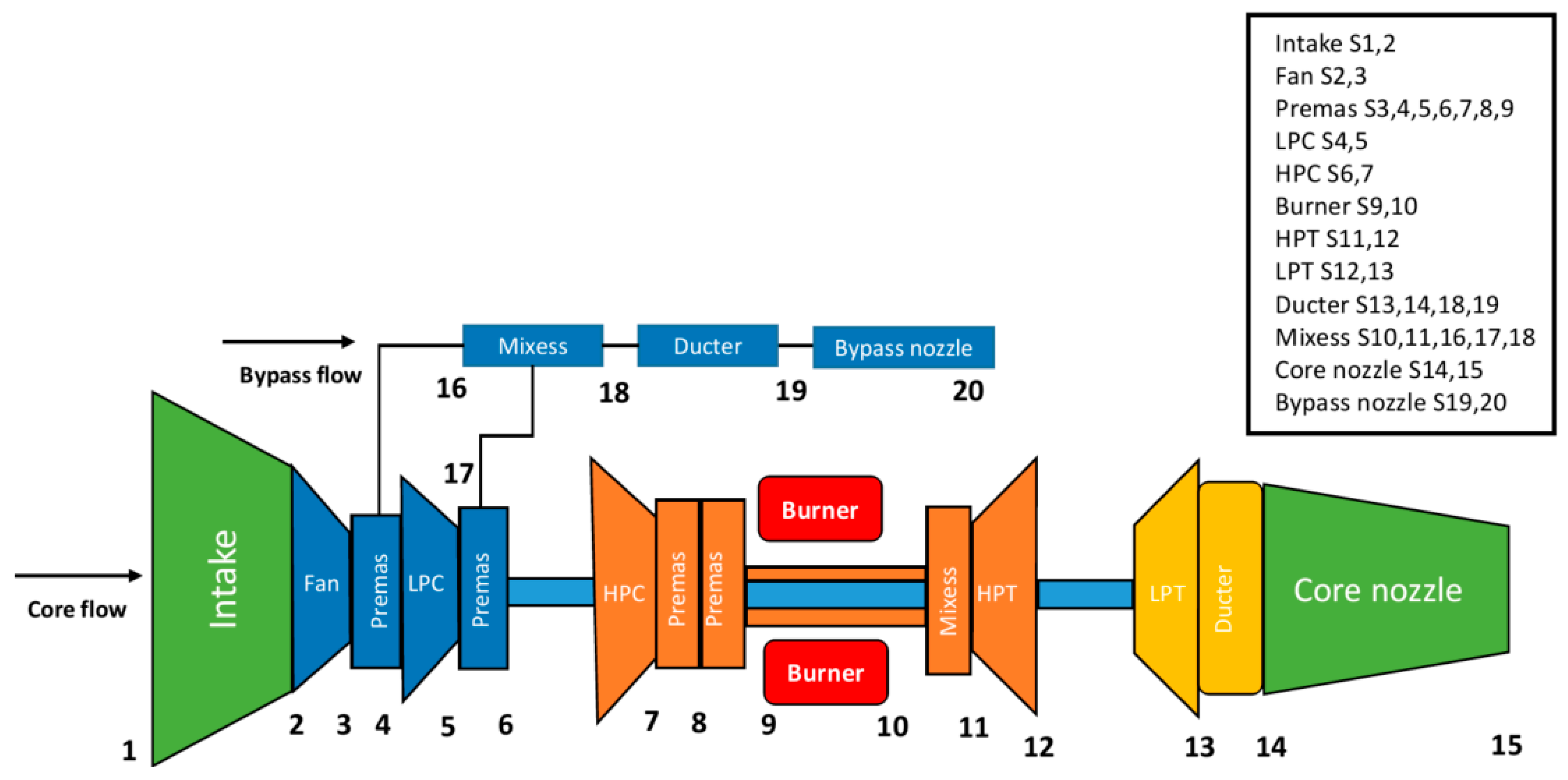
3.1. Model Description

The fan, bypass ducting, and the first two stages of the LPC were selected for this study as components of a research aeroengine inspired by NASA’s E3 engine [27,28,29]. Furthermore, the model was originally assembled by a previous research work at Cranfield University. Geometric details showing the locations of the airfoils, which define the blading as well as the annular definition curves of the engine components modelled, are presented in Figure 1a together with the CFD domain employed in the simulations, Figure 1b, and detail of the blading of the IGV and the first two stages of the booster compressor used for the surface roughness simulations, Figure 1c. The design parameters at the design point (DP) are shown in Table 2.

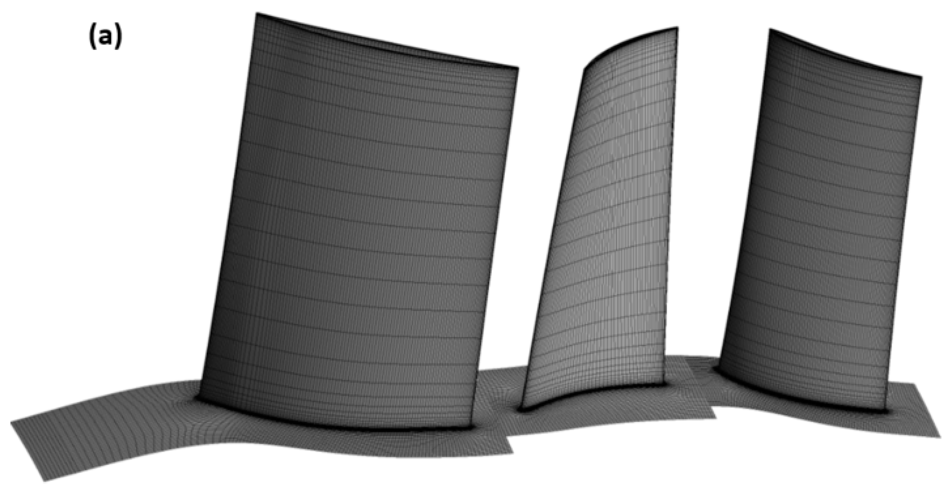
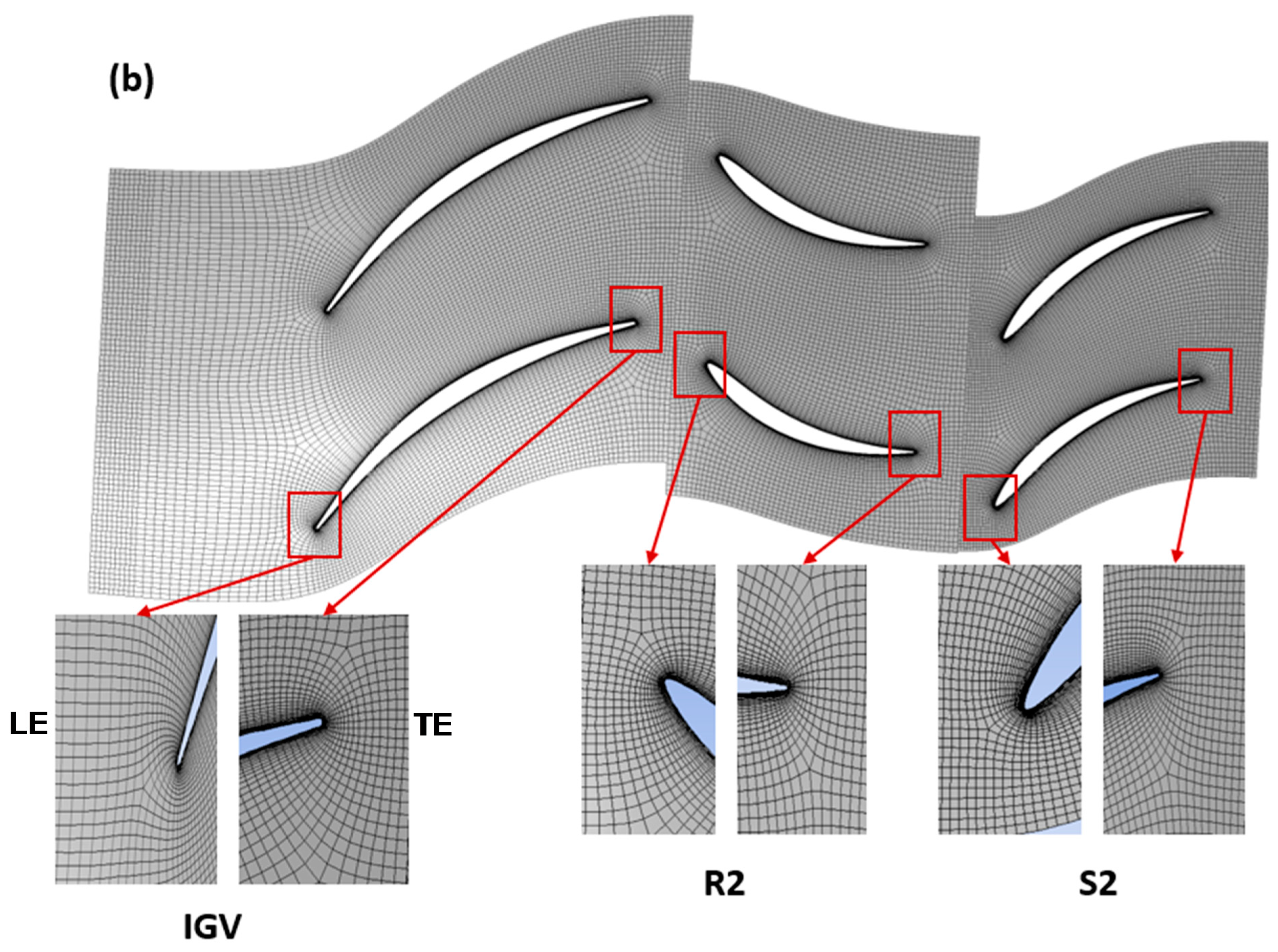
3.2. Mesh Generation and Model Verification

A structured mesh was generated using the Turbogrid meshing tool, CFD, CFX 19.1V (ANSYS Inc, Canonsburg, PA, USA), which is part of the CFD, CFX 19.1V (ANSYS Inc, Canonsburg, Pa, USA) suite. The mesh sensitivity was carried out on all of the computational domains. An example of the surface mesh on the hub, and details of the LE and TE at 50% blade height are shown in Figure 2 for the IGV, R2, and S2 blade rows.
A mesh dependency study was performed at the LPC DP, and the results are presented in Table 3. The R2 component was selected for the comparison objective in Table 3.
The medium-mesh was selected in this study as it offers an adequate resolution while keeping the computational costs relatively low. The number of nodes of each simulated component is shown in Table 4.
The model verification involves the examination of the dependency of the results on the density of the meshes employed.
The well-known Grid Convergence Index method (GCI) [40] has been employed in this study. The GCI technique is based on the Richardson extrapolation (RE) concept. The GCI method defined herein is a suitable procedure, evaluated over numerous CFD cases, and it is the most dependable method available for the evaluation of numerical uncertainty [40]. To achieve the estimation of the discretization error, the procedure is listed as follows:
Define the cell size (h) for the three mesh sizes utilised in the study by
h = 1 N   i = 1 N ( Δ   V i ) 1 / 3
where, N 1, N 2, and N 3 are the total number of cells for the coarse, medium, and fine cases, respectively, and Δ V i represents the volume.
Calculate the values of the critical variables that are considered an objective of the numerical study. Here, the pressure ratio (PR) values for the coarse, medium, and fine cases, which are represented as 1 ,   2 ,   3   , respectively, were employed for the comparison.
Determine the apparent order p by using the following Equations
p = 1 ln ( r 21 )   | ln | ε 32 ε 21 | + q ( p ) |
q ( p ) = ln ( r 21 p S r 32 p S )  
S = 1   . sgn   ( ε 32 ε 21 )
where, r 21 ,   r 32 represent the grid refinement factor as r 21 = h 2 / h 1 and r 32 = h 3 / h 2 , and ε 21 = 2 1 and ε 32 = 3 2 .
Determine the extrapolated values ( e x t 21 ) using
e x t 21 = ( r 21 p   1 2 ) ( r 21 p 1 )
Determine the error estimation from
e a 21 = | 1 2   1 |
e e x t 21 = | e x t 21 1   e x t 21 |  
G C I F i n e 21 = 1.25   e a 21 r 21 p 1
where e a 21 represents the approximate relative error, e e x t 21 represents the extrapolated relative error, and G C I F i n e 21 the fine-grid convergence index.
The calculations of the discretization error are listed in Table 5. The results reported the numerical uncertainty in the fine-grid solution for the PR as 3.5%.

3.3. Boundary Conditions and Convergence Criterium

A schematic representation of the computational domain together with its dimensions relative to the fan blade chord at midspan is presented in Figure 3. The inlet and outlet boundary conditions are applied at locations identified in Figure 3. The location of these boundaries is placed away from the turbomachinery components in order to ensure that the local flow is developed according to CFD good practice.
A single periodic blade passage of every LPC component was analysed at the DP. The boundary conditions were set as follows:
(1)
The stator domains of the EGV, IGV, S2, and S3 were set as stationary.
(2)
The rotor domains of the fan, R2, and R3 were set as rotating at 4215 rpm.
(3)
All walls were set as no slip.
(4)
At the inlet: the stationary frame total pressure P 01 = 101.325 KPa, and total temperature T 01 = 288.15 K were prescribed. The turbulence intensity was set at 5%.
(5)
Mixing planes were used as the interface between stator and rotor rows.
(6)
At outlets, bypass and booster, average static pressure was specified with values adjusted by trial and error to enable these two components to pass the target m ˙ .
All cases converged with residual values of mass below 10−5 whereas the residual values of momentum dropped below 10−4.

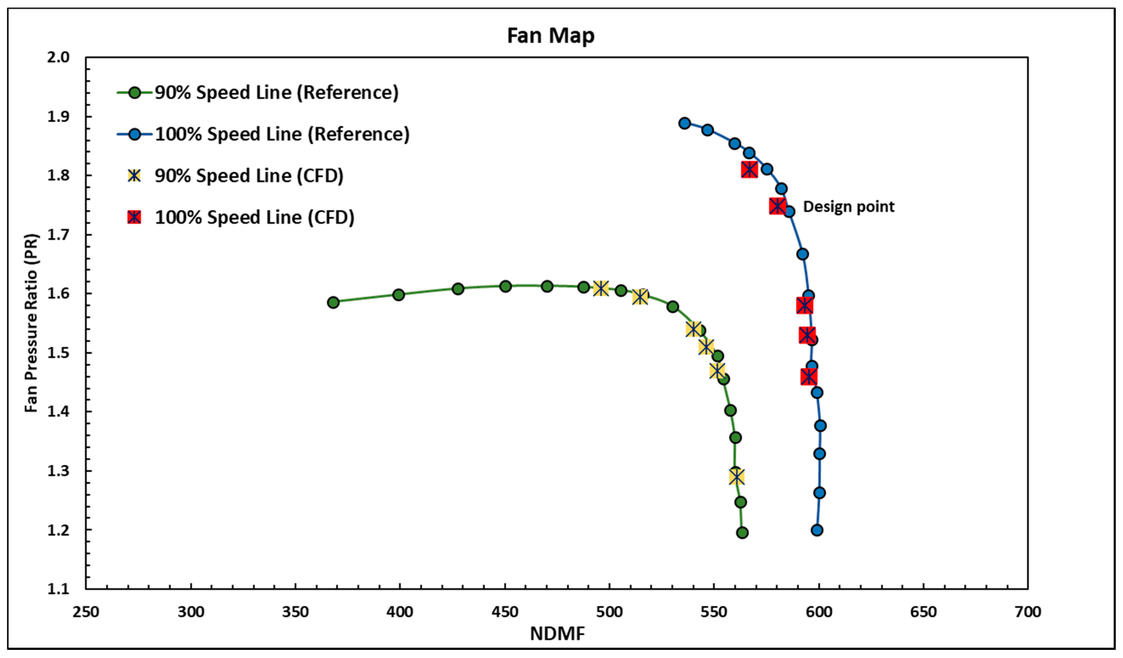
3.4. CFD Results Comparison

The CFD and Turbomatch results were examined against the NASA E3 reference data [27,28,29]. Furthermore, the CFD results were compared against the design parameters of the available fan rotor data of the E3 engine [29]. The outcomes are verified in terms of the PR and the NDMF. The results obtained from the CFD simulations at both 90% and 100% speed-lines presented a very good match with the reference data, as shown in Figure 4. Additionally, it was found that the maximum deviation of the CFD results compared to the design objective was 1.9% of NDMF at the 100% speed-line.
Furthermore, a comparison study was performed to compare the results of the numerical simulations of the modelled booster stages of the research engine at the design point. The results obtained that focus on the variation of the m ˙ , PR, exit temperature ( T 2 ), and the η i s of the second stage of the LPC are listed in Table 6. The outcomes demonstrate good agreement as the variation between the CFD results and the design calculation’s values are less than 4%.

4. Results and Discussion

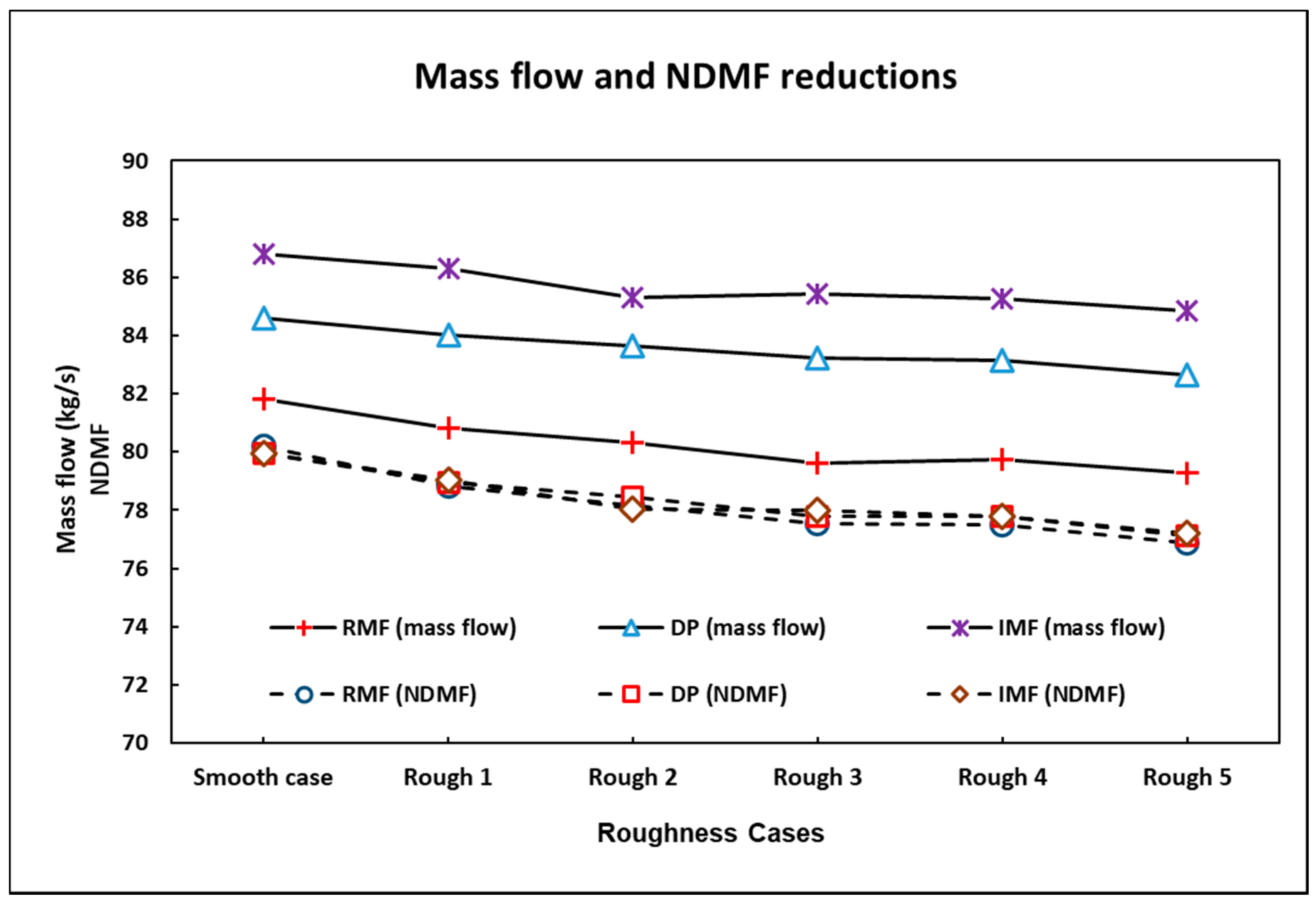
4.1. Effect of Roughness Variation on Engine Mass Flow

Three different operating points located on the 100% speed-line have been selected for the examination of the results: reduced (RMF), design point (DP), and increased mass flow (IMF) of 81.8 kg/s, 84.6 kg/s, and 86.8 kg/s, respectively. To examine the impact of increasing the surface roughness of LPC blades, NDMF, PR, and the η i s were evaluated. The computed cases are introduced in Table 1. Furthermore, the NDMF parameter is introduced for the purposes of comparing different types of compressors [41,42]. The simulation results of the m ˙ and the NDMF for the smooth case and the different roughness cases are shown in Figure 5. Each line is labelled by the corresponding operating point. Moreover, the outcomes demonstrate that increasing surface roughness reduced the m ˙ and the NDMF. The reduced mass flow operating point was most affected by surface roughness, and the deviation at this operating point was 3.2% and 4.1% for the m ˙ and the NDMF, respectively. Therefore, the observed degradation can be ascribed to the increase in blockage and, hence, a reduction in effective throat areas.
The increase in losses in the flow can result in a significant drop in the LPC’s PR and efficiency, reducing, therefore, the power output of the GTE. The numerical predictions of PR and efficiency reductions of the compressor at the 100% design speed, taken at the three different operating points are presented in Figure 6 and Figure 7, respectively. It can be observed that the values of the PR and the η i s of the computed stages reduced progressively as the roughness conditions of the blades increased. The maximum reduction in PR of 3.1%, corresponds to the highest surface roughness at RMF condition as shown in Figure 6.
In comparison, the maximum reduction in the efficiency of 7.7% was found at the operating point corresponding to IMF. A very similar result was obtained for the compressor efficiency at the DP as shown in Figure 7.

4.2. Effect of Roughness Variation on Compressor Aerodynamics

CFD predictions in terms of flow characterisation are presented in this section. The results listed in this section correspond to the DP.

4.2.1. Effect on Flow Structure

Increasing the blade’s surface roughness has a noticeable effect on the flow field, especially across the blade SS of the stators and rotors. In order to demonstrate the impact of surface roughness on the LPC components, the IGV is selected.
The wall shear stress on the SS of the IGV is plotted in Figure 8 below for the smooth and the Rough 5 cases. As is apparent, there is some inward radial migration near the end walls with the occurrence of a sizable hub corner stall, which starts at the midchord position for both roughness cases.
As can be observed from Figure 8, the increase in roughness is accompanied by a rise in the spanwise values of the wall shear stress. This effect is more clearly observed by plotting the chordwise distribution of this quantity at midspan, Figure 9.
The chordwise distribution of wall shear stress shown in Figure 9 provides evidence not only of the bulk increase of this quantity but also of its evolution from the leading to the trailing edges. The average increase in wall shear stress, computed over the SS, is around 85%. Regarding the differences between the Rough 5 and the smooth case distributions, a general increase in the SS and the PS values with roughness is noted. Interestingly enough, the high roughness case is associated with a decrease in wall shear stress in the latter section of the chord with respect to the smooth case.

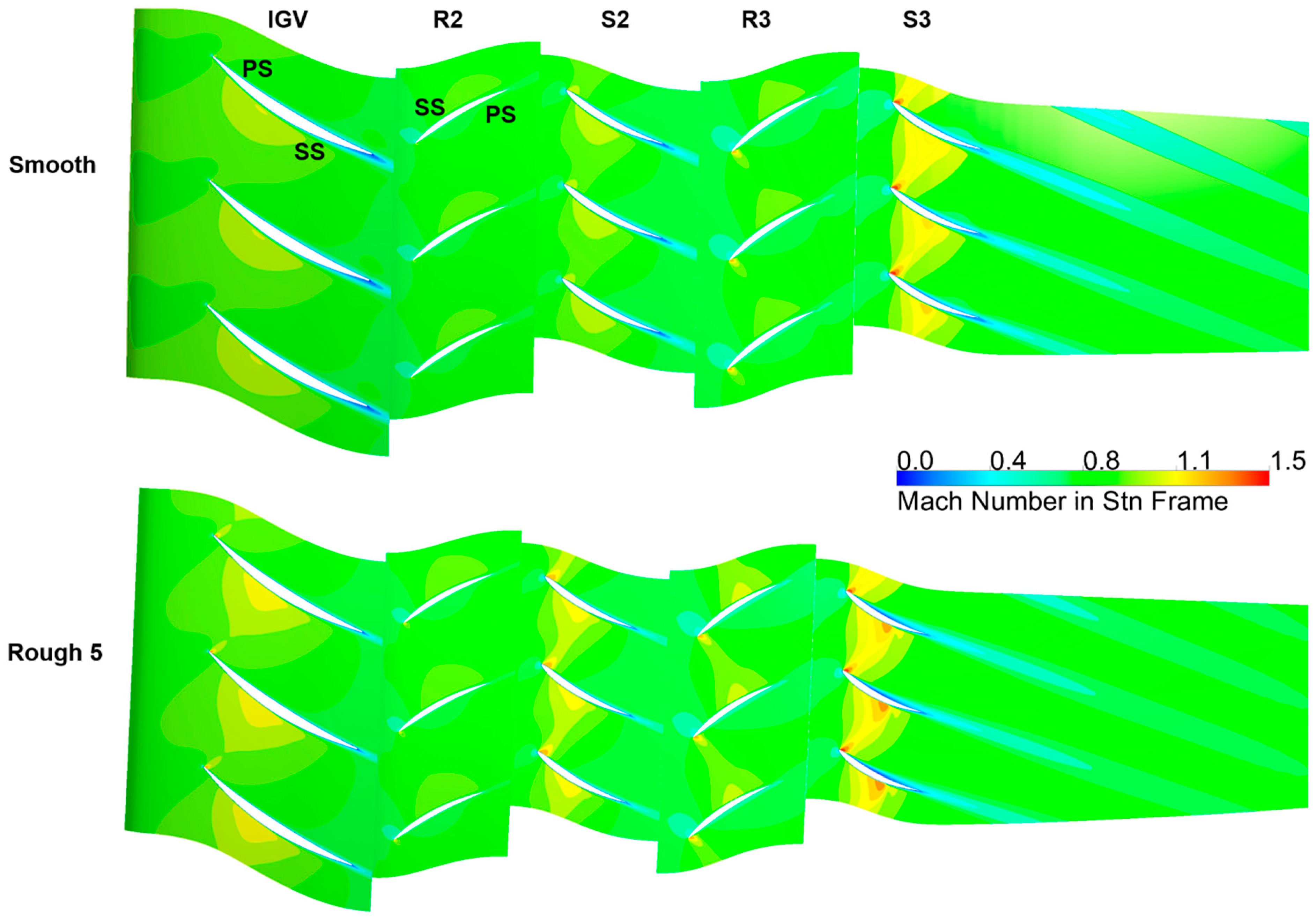
4.2.2. Effect on Mach Number Distributions

The distribution of relative Mach number at the DP for a smooth and rough case (Rough 5) at 50% blade span is presented in Figure 10. The flow is subsonic throughout except for some regions near the leading edge and towards the latter stator midchord position. A comparison between the smooth case and the highest roughened case leads to the identification of expanded patches of detached flow near the TE regions. In the roughened case there is a reduction in the extent of the high Mach number regions throughout, as was also observed by Sun et al. [26]. For roughened cases, in comparison to the SS of the blades, the PS is associated with a lower value in terms of the distribution of Mach numbers due to lower flow acceleration, which creates a thinning turbulent boundary layer accompanied by suppression of boundary layer turbulence as observed in reference [43]. These results indicate that the surface roughness has a minor effect on the Mach number distributions for the computed cases. However, the increases in surface roughness do result in increases in the flow blockage, which in turn contribute to the observed performance deterioration of the LPC in a manner similar to that reported in reference [44].

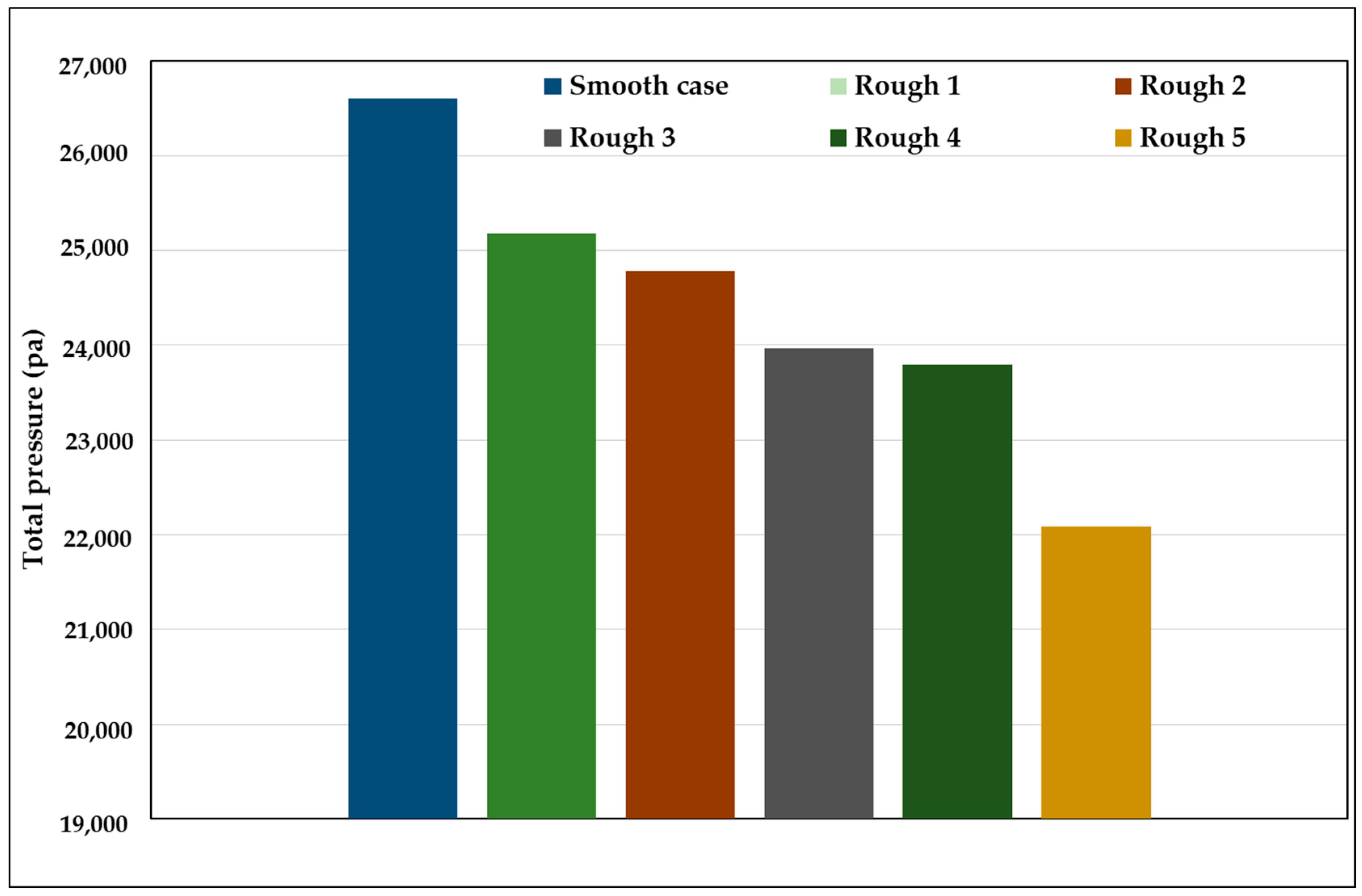
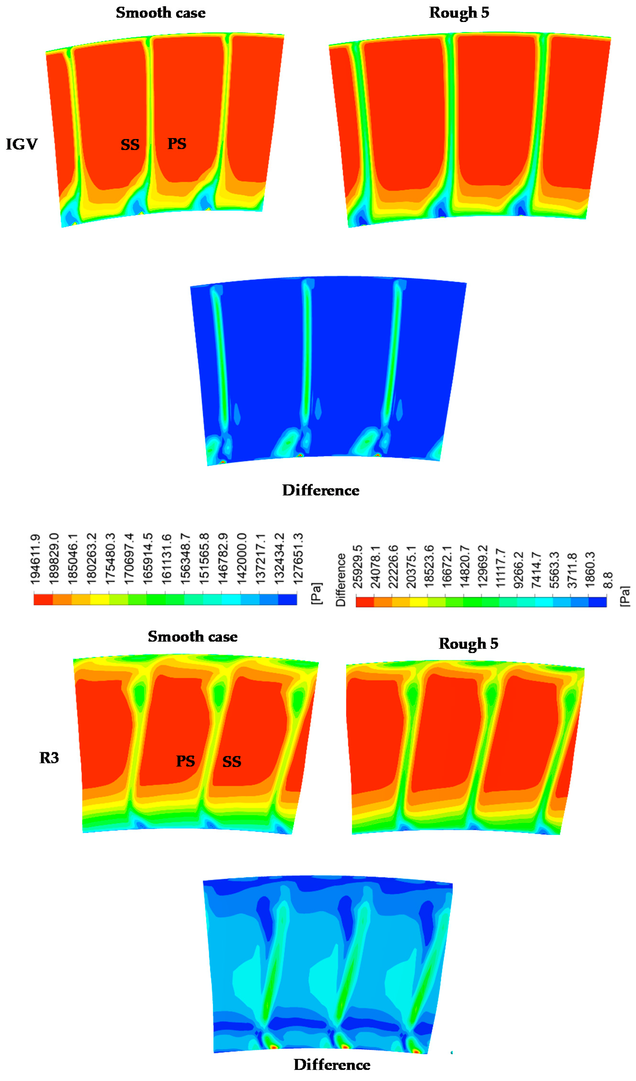
4.2.3. Effect on Total Pressure

The total pressure distribution of the flow with different roughness scenarios showed that the pressure loss is amplified by increasing surface roughness. The loss in total pressure is reported with reference to the decrease in total pressure rise in the booster calculated as a difference between the value computed downstream of S3 and the average value calculated upstream of the IGV, Figure 11. As can be observed in this Figure, the introduction of roughness, even for the lowest value (Rough 1 case), is associated with a reduction in the total pressure rise (5.1%), which is considerably larger than that observed when the roughness doubles between 15 and 30 µm (1.5% between Rough 1 and 2, respectively). Contour plots of the spatial distribution of total pressure at the IGV and R3 blade row exit, taken downstream of both components, for the smooth and Rough 5 cases, are shown in Figure 12. The results demonstrate a thickening of the wakes between the smooth and the roughened case. This observation is valid both for the IGV and the rotor domain. For the IGV case, low momentum core of the hub-corner stall is further developed with roughening of the blades. The difference plots indicate the areas and magnitude of roughness effects, showing that the total pressure is mainly influenced in the immediate vicinity of the blade surface, particularly at the suction side. The end wall regions, in turn, remain mostly unaffected.

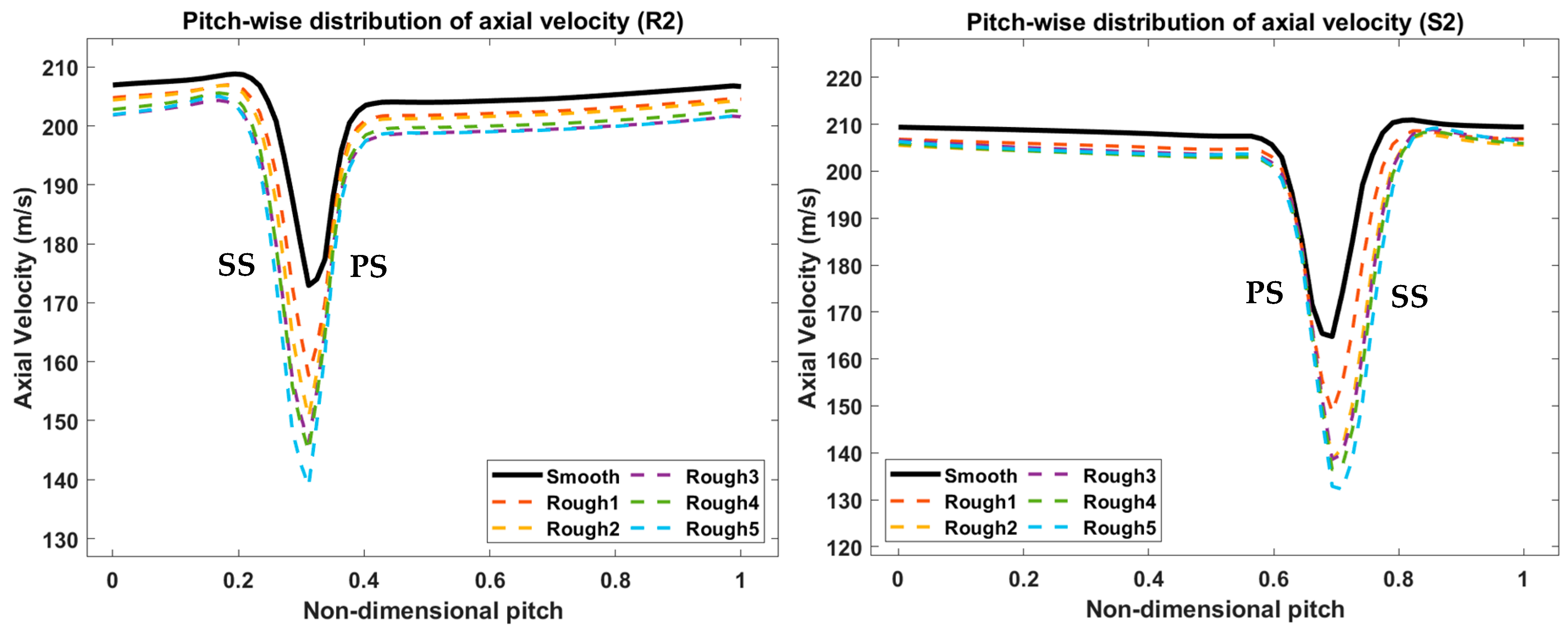
4.2.4. Distribution of Axial Velocity

The distribution of axial velocity is examined in this section. The introduction of roughness has a marked effect on the axial velocity deficit associated with merging boundary layers in the wake region. The axial velocity distribution downstream of R2 and S2 versus non-dimensional pitch is plotted in Figure 13. The increase in roughness leads to a combined effect of increasing the depth of the wake together with thickening of the boundary layer, especially at the SS region. It is noteworthy how the low roughness case (Rough 1) produces a substantial thickening of the wake, a process that is then further reinforced with increasing roughness, although at a considerably reduced rate. Regarding the velocity defect, the introduction of roughness is associated with an increase in the depth of the wake, which ranges from 12% for the Rough 1 case to about 24% for the Rough 5 case when considering the R2 component. A similar magnitude of the velocity drop was observed in the stator S2.

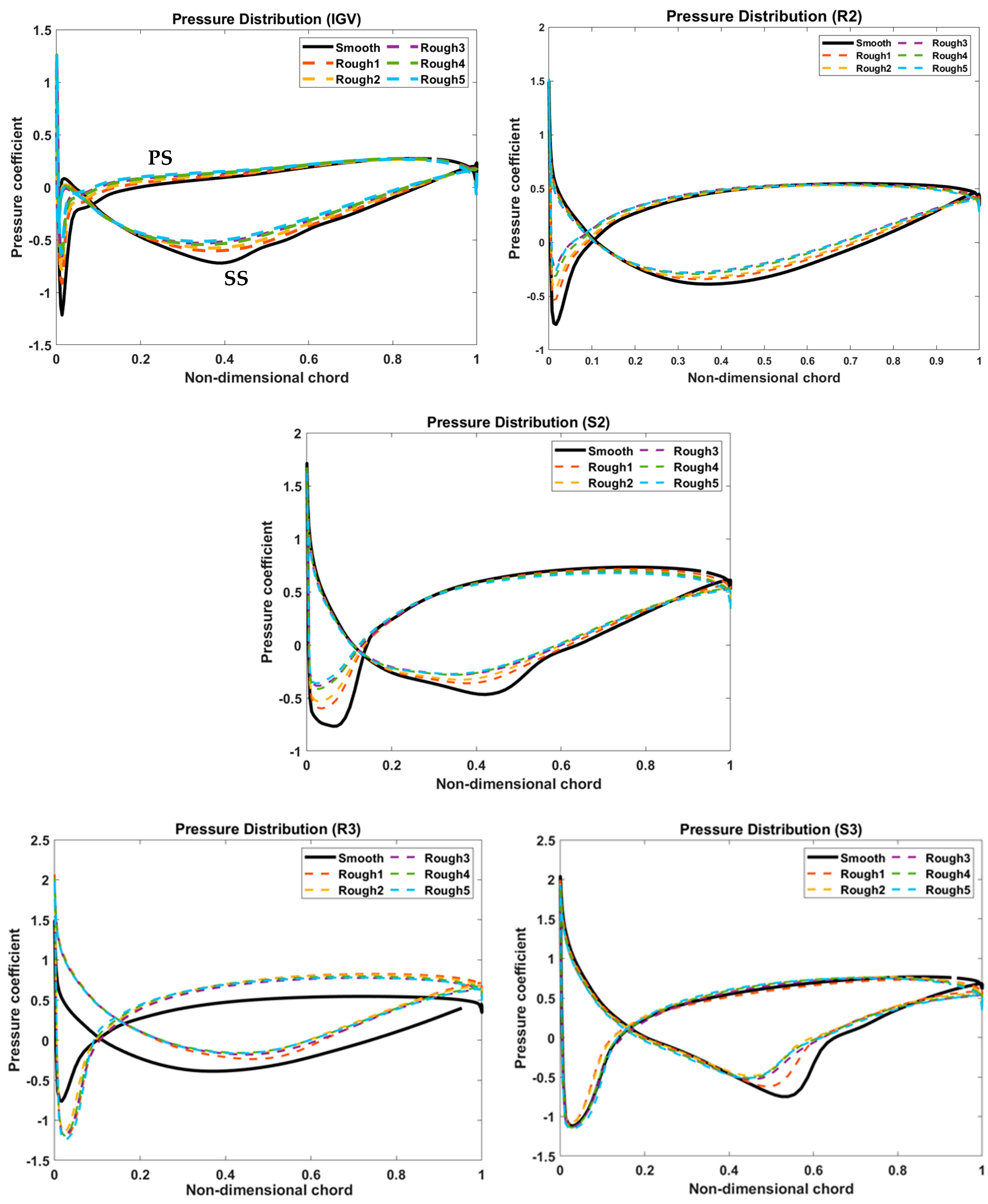
4.2.5. The Pressure Coefficient

The static pressure coefficient ( C p ) is a key parameter providing information on the aerodynamic loading of the blades. In addition, it can supply information regarding the occurrence of shocks and the chordwise variation of losses. The static pressure coefficient is given by the following expression [45]
C p = P s P 1 P 01 P 1
where P s is the static pressure of the blade, P 1 is the upstream static pressure used as reference, and P 01 is the inlet total pressure.
The C p distribution around the blades at midspan is presented in Figure 14 for the IGV, R2, S2, R3, and S3. As was noted before, the SS tends to be more affected by the roughness. Except for R3, the PS exhibits a reduction in the LE pressure spike extending over the first ~20% of the blade chord. The severity of the reduction correlates with the level of roughness, although, somewhat surprisingly, the values of high roughness and the intermediate ones, i.e., Rough 3 and Rough 5, produce relatively similar distributions. It is noteworthy that the introduction of roughness, even Rough 1 ( k s = 15 µm), yields a considerable departure from the smooth surface. The SS variation with roughness extends over the bulk of the chord and is again well correlated to the level of roughness. The last stage provides the exception to this general observation. The pressure drop observed in S3 related to the shock location is attenuated with the introduction of roughness. The pressure distributions at the second rotor blade, R3, exhibit a different behaviour compared to the other LPC blades. The observed difference is due to the position of the rotor stagnation point. In the rear rotor blades, the flow impinges on the SS at a positive incidence. Thus, flow deviation is facilitated by surface roughness, promoting separation at the blade SS, which was also observed by Zhihui and Yanming [22].

4.3. Turbomatch Performance Tool

Aeroengine performance simulations are frequently utilised to examine the engine behaviour at different operating conditions. Such simulations can be beneficial during the engine development process in evaluating performance, assisting component design, testing data, and optimizing the engine controls, associated with decreased design and development costs [46]. Therefore, a robust design is essential for the engine performance design stage [47]. In this research, the thermodynamic cycle performance calculations were carried out by utilising an in-house tool—Turbomatch. Turbomatch is a performance software developed by Cranfield University for design point (DP) and off-design (OD) analysis of GTEs. The performance of GTEs is determined by utilising scaled maps of the compressors, combustion chambers, and turbines. Turbomatch relies on several subroutines to simulate the performance of the GTE’s components. The user can assemble the modules together to create an engine model with the required specifications. This allows for a considerable degree of flexibility to examine alternative GTE arrangements and operating conditions. A comprehensive description of the working principles and implementation of the Turbomatch suite can be found in [48,49,50].
In this study, a Turbomatch model was created according to the available technical data of the E3 engine [27,28,29]. To examine the blade surface degradation effects on engine performance, the PR, mass flow at inlet ( M ˙ i n ) , and efficiency were adjusted according to the degradation level. The scaling factor (SF) of these specific parameters needs to be utilised against the corresponding values of the standard map as follows [51]
S F P R = P R D P 1 P R D P   M A P 1
S F η i s = η i s D P η i s D P   M A P  
S F N D M F = N D M F D P N D M F D P   M A P
NDMF = M ˙ i n 101,325   ( Pa ) P 01   T 01 288.15   ( K )
where PR represents the pressure ratio, η i s the isentropic efficiency, NDMF the non-dimensional mass flow, M ˙ i n the mass flow at the inlet, P 01 the total pressure, and T 01 is the total temperature.
The SFC, TET, and EPR were calculated to analyse the engine behaviour under the degradation phenomenon. A schematic of the research engine is shown in Figure 15, representing the individual components called ‘bricks’ in Turbomatch: Intake, Fan, Bypass duct/flow splitter for bleed (Premas brick), LPC, area of mixing of two flows (Mixess brick), afterburner/intercooler duct (Ducter brick), Bypass nozzle, high pressure compressor (HPC), Burner, high pressure turbine (HPT), low pressure turbine (LPT), and Core nozzle. The bricks are linked together, with interfaces known as stations.

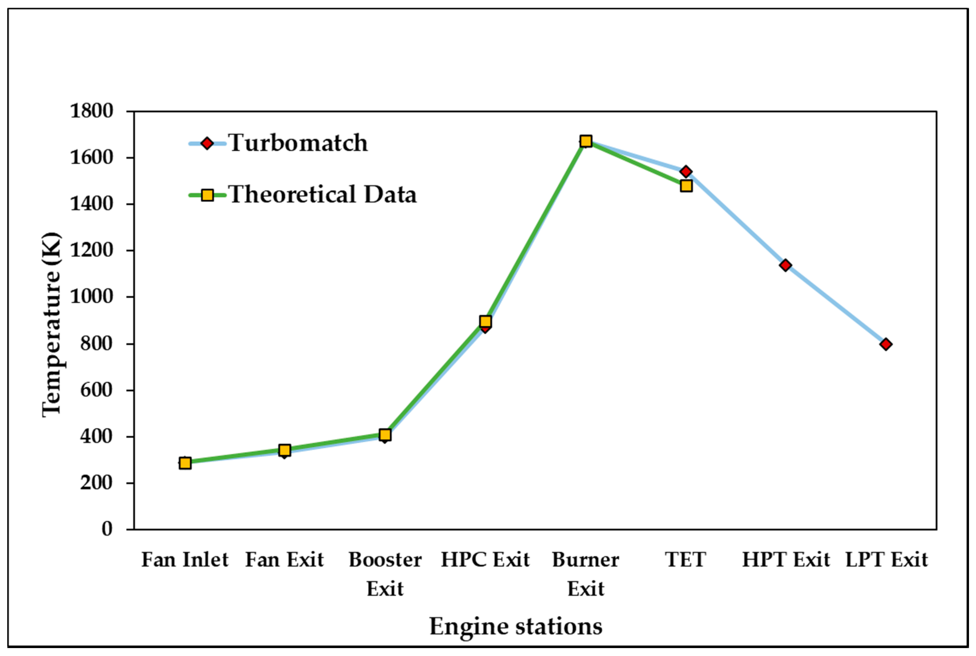
Turbomatch Model Validation

A comparison of Turbomatch results against the E3 reference data [27,28,29] was performed. The verification is based on the temperatures at each engine station for the 100% speed-line, as shown in Figure 16.
The temperatures provide a good indication of whether the GTE meets the design requirements. In particular, the maximum cycle temperatures influence the maximum overall thermal efficiency of the GTE and can indicate the design matching of the GTE components [52]. The comparison was performed by using the available data for the exit temperatures of the E3 components in terms of the fan, LPC, HPC, burner, and TET. The HPT temperatures and the LPT are left without comparison due to the lack of reference data for the turbine section of the E3 engine. The results show a satisfactory agreement. The maximum discrepancy between the Turbomatch results and the reported design data was found at the TET to be less than 4%.

4.4. Turbomatch Performance Results

To analyse the performance implications of increasing surface roughness in the LPC, a thermodynamic study was carried out using Turbomatch. To estimate the degradation levels of the two stages of the LPC that have been computed in this study, the research engine booster has been split into two parts. The simulated stages, as well as the latter two stages of the LPC were scaled by Turbomatch as two separate components. The modelling of the degradation in Turbomatch involves specifying the reduction in PR, NDMF, and the η i s as handle parameters affecting the performance of the compressor. The values are taken from the CFD analysis. The input data representing the influence of the roughness conditions on the engine performance variables are presented in Table 7. The outputs of the Turbomatch model are expressed through the EPR, SFC, and TET.

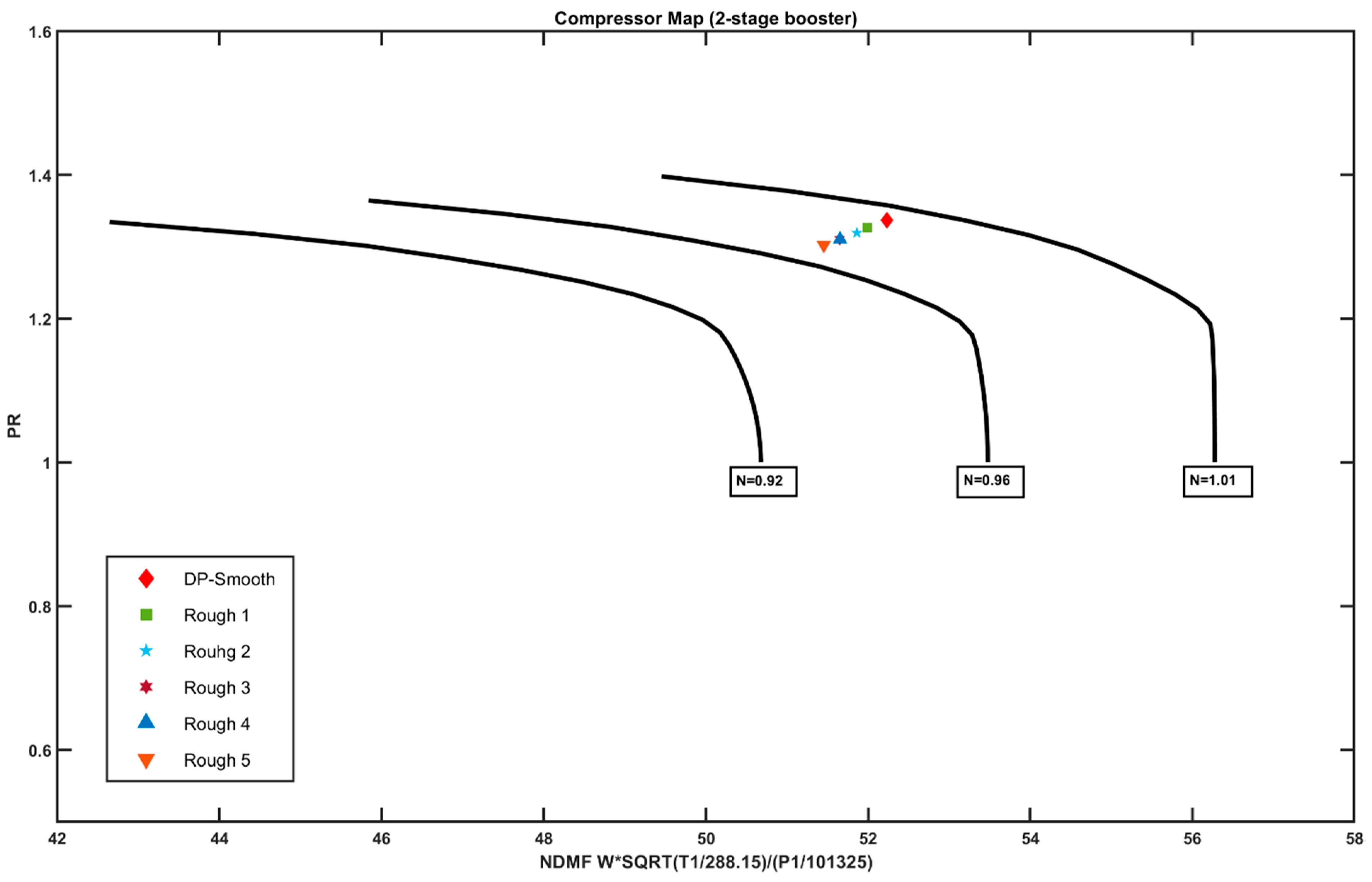
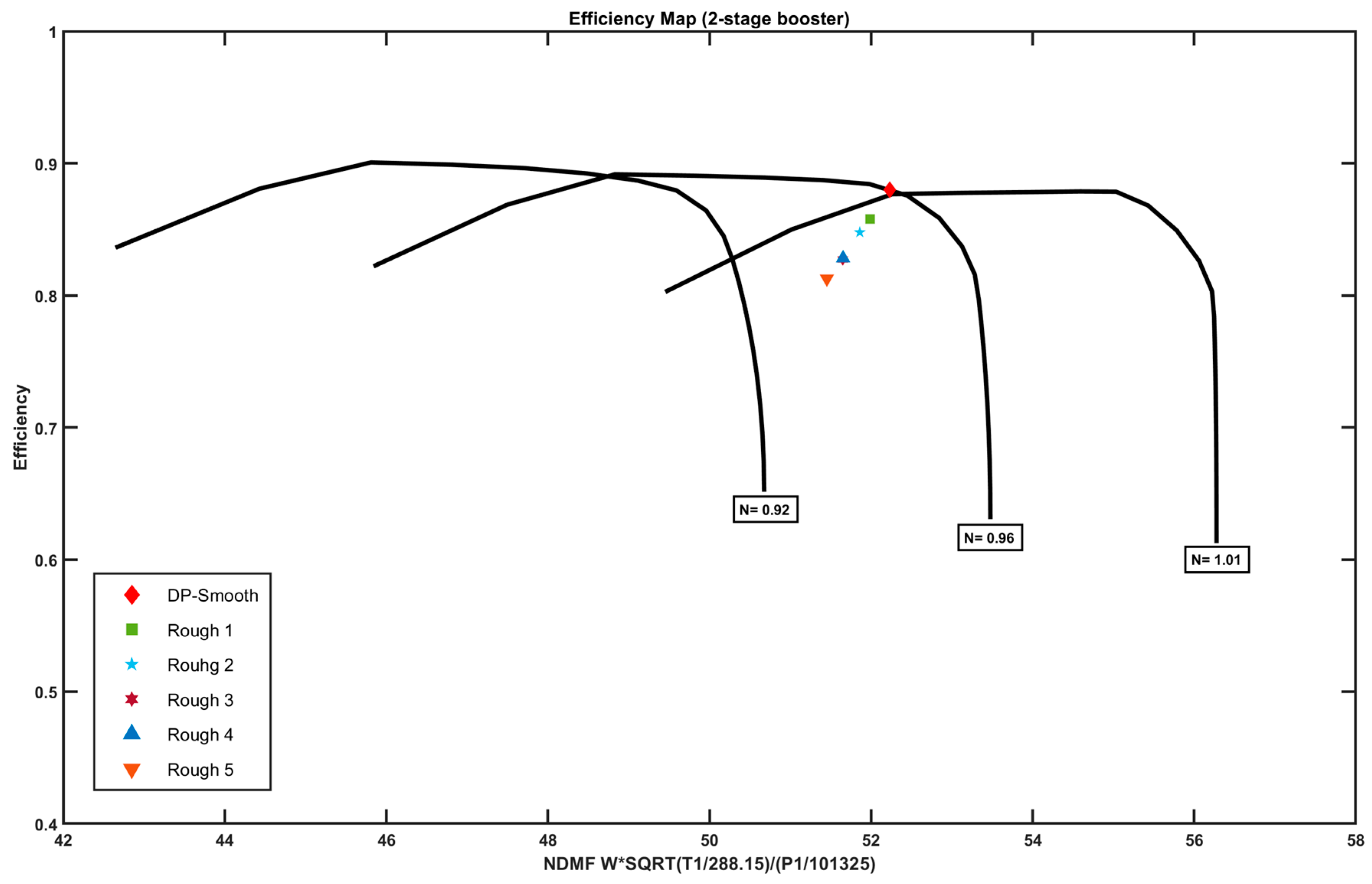
4.4.1. Effect on Compressor Maps

By applying the levels of degradation specified in Table 7, the performance implications of the roughened conditions were examined. The analysis of the roughened stages was carried out at the DP. The variation in the characteristic maps of the first two stages of the LPC is presented in Figure 17 and Figure 18 regarding the PR and the isentropic efficiency against the NDMF. The black lines in these plots correspond to the values obtained at three rotational speeds (N) indicated in the figures. It can be noticed that the smooth case values of PR and isentropic efficiency corresponding to DP are obtained at 100% N. The results indicate that if surface roughness is increased, the DP is shifted away from its initial position on the map, and the compressor operates at a reduced mass flow and PR. As shown in Figure 17.
Similarly, the DP is shifted away from its initial position on the map, while the surface roughness is increased and the compressor operates at a reduced mass flow and efficiency as shown in Figure 18.
As observed previously, setting the roughness at 15 µm and 30 µm presents a marked difference in the shift of the corresponding PR and efficiency points in reference to the smooth case. This indicates that the compressor is more sensitive to the introduction of roughness than to its increase.
Roughness limits are, in practice, controlled by the hardness and the mechanical specifications of the tested material, even if degraded. According to Hamed [20], for turbomachinery applications, the blade’s surface roughness does not increase beyond a given limit due to the physics of the solid particle erosion (SPE) process that induces the roughening of the blades. Thus, the impact of surface roughening will be limited to a threshold k s value somewhere around the 45 µm mark according to the references [20,38]. The examination of cases with k s   > 45 µm was performed in order to investigate the behaviour of the compressor in a situation where alternative blade material properties might enable higher values of roughness than what is commonly encountered with current manufacturing materials and techniques.

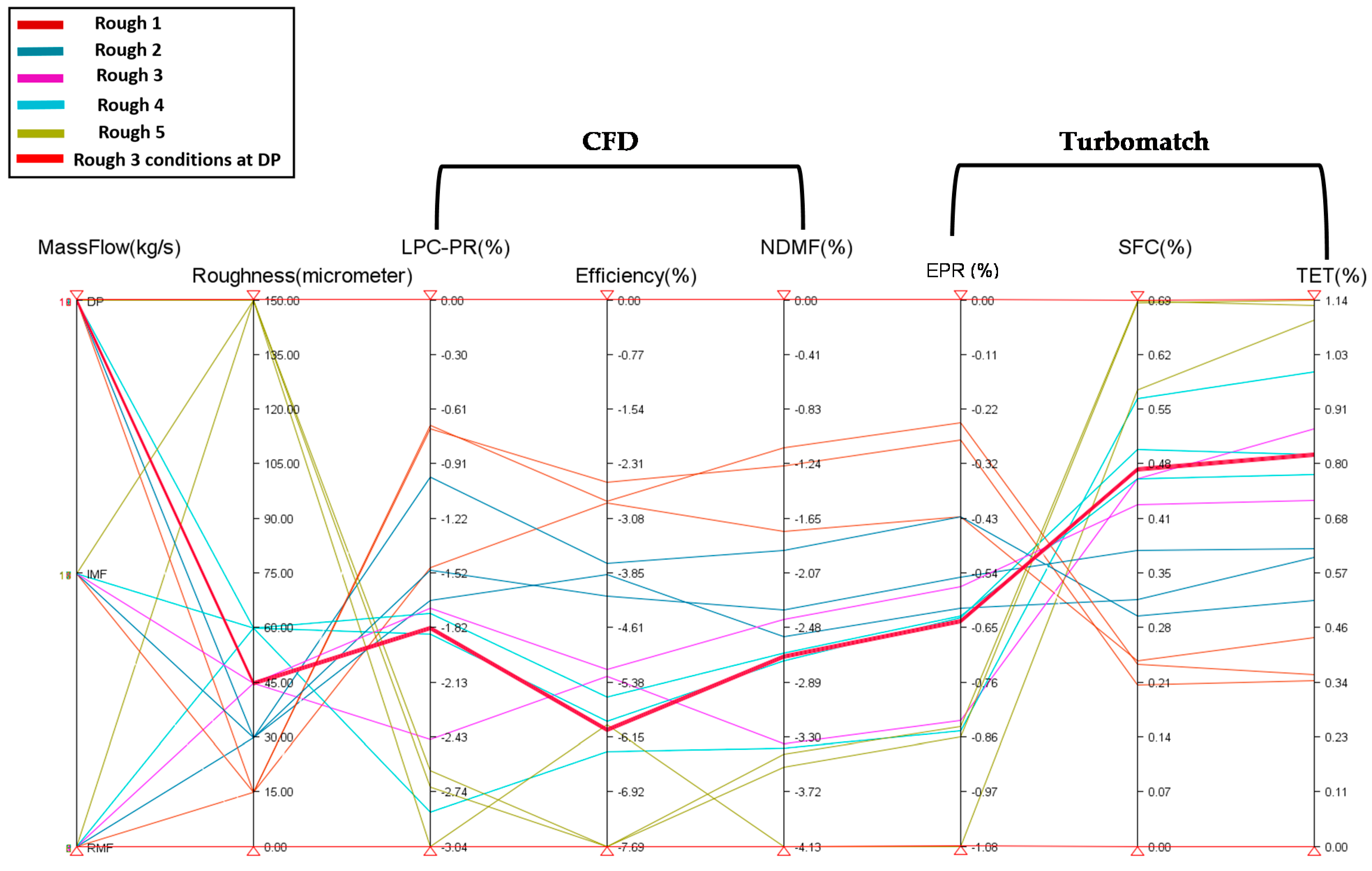
4.4.2. Effect on Cycle Parameters

The increased surface roughness affects the EPR, SFC, and TET of the research engine. The impact of increasing the surface roughness of the EPR and SFC are tabulated as a percentage, while the TET is shown as a change in temperatures (Δ) compared to the smooth case, Table 8.
Although the engine performance changes are relatively minor for the cases studied, they represent significant cycle degradations resulting in a noticeable drop in EPR and attending increase in SFC, affecting the economics of the operation. Although the increase in TET is in absolute terms not very significative for the low roughness values, it represents nevertheless a tangible degradation of the GTE since even minor increases in TET are associated with creep life reductions and, hence, affect the durability and maintenance requirements of the engine.
In order to highlight the implications on the whole engine performance along with the LPC performance, a combination of the Turbomatch and CFD results is shown in Figure 19. The results are juxtaposed using a parallel coordinate chart to show the simultaneous effects on each variable by varying the surface roughness in the LPC’s first two stages.
It can be seen that the large degradation of the LPC predicted by the CFD analysis, impacts in a less substantial manner the overall cycle performance in terms of SFC, TET, and EPR. Taking as an example the Rough 3 condition at DP (indicated in Figure 19 through a thick red line), its impact on the first two stages’ PR is in the order of a 1.8% drop, 6.1% drop in isentropic efficiency, and 2.7% drop in NDMF, whereas the corresponding rise in the overall cycle SFC is 0.48% and in TET is 0.8%, together with a drop in EPR of 0.61%. These values are valid for the reduced section of the booster model, which is in any case the part of the core compressor system more directly affected by solid particle erosion (SPE) and must not be taken to represent the degradation effects of the full compressor, and are, hence, representative of a subset of a wider GTE deterioration phenomenon.

5. Conclusions

This study examined the aerodynamic and engine performance implications of increasing blade surface roughness in the first two stages of a low pressure compressor utilising the design parameters of the E3 engine. Blade roughness stemming from the operation of GTEs in dust laden atmospheric conditions is known to occur in the first stages of the compression system. This investigation sought to quantify the blade surface degradation of the first two stages with an examination of their impact for the thermodynamic cycle. The results showed that uniformly increased surface roughness of the blades significantly reduces the compressor efficiency and PR, impacting the performance of the whole thermodynamic cycle. The qualitative and quantitative outcomes of this study are as follows:
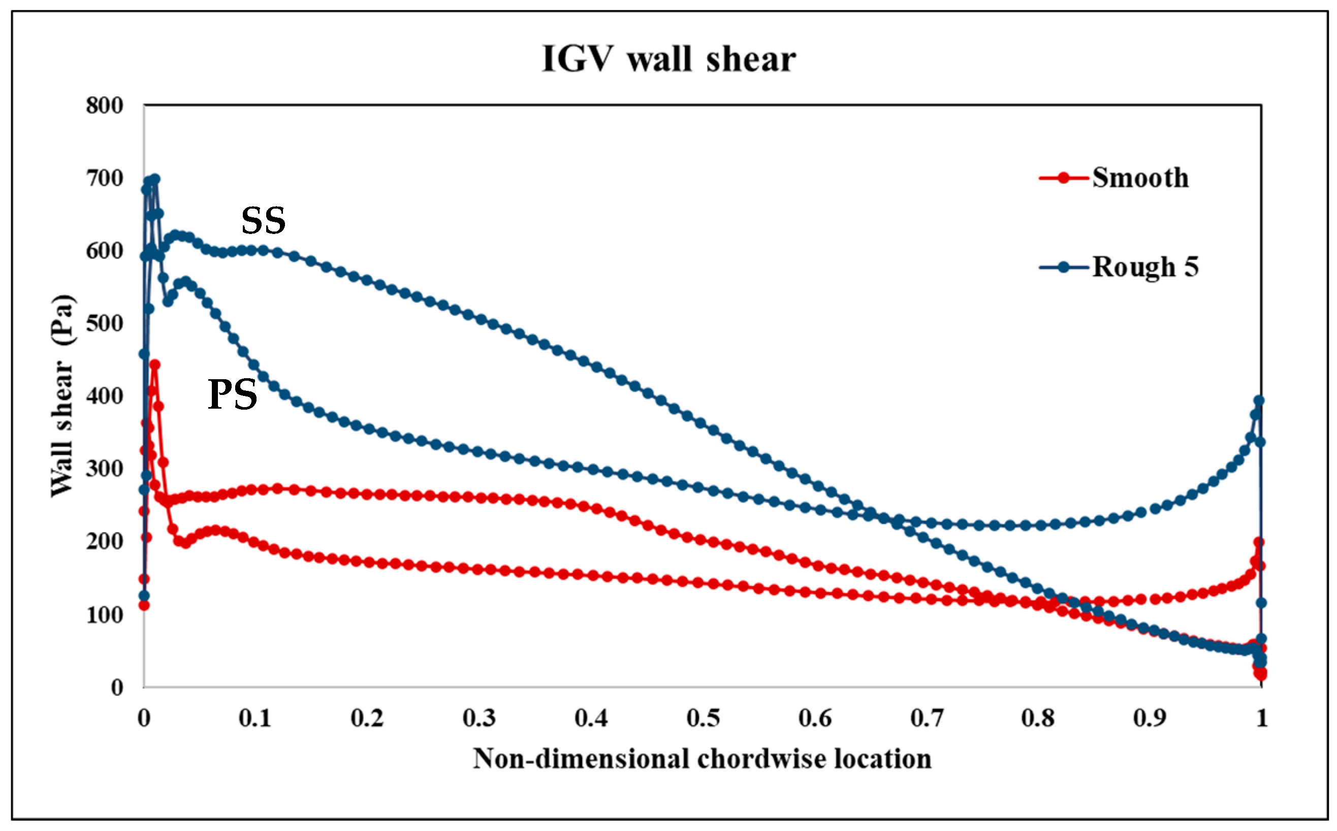
  • The simulations employed uniformly roughened blades notwithstanding the fact that it is known that rotor and stator blades experience different levels of roughness in the suction and pressure sides when compressors are exposed to SPE conditions. This modelling approach is justified on the grounds that the pressure side of both stators and rotors is largely insensitive to the variation in whole blade roughness level as is evident from the analysis of Figure 13.
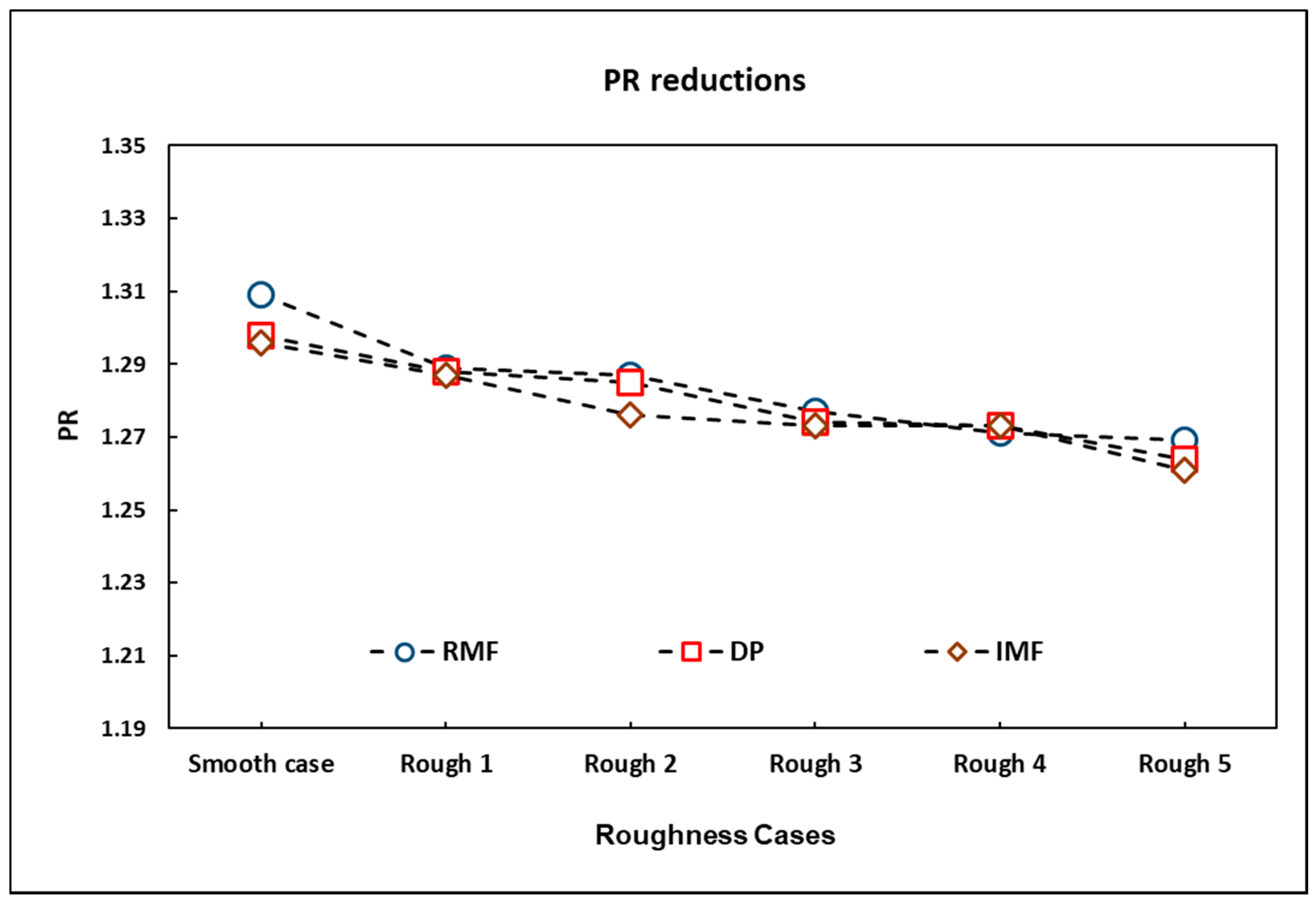
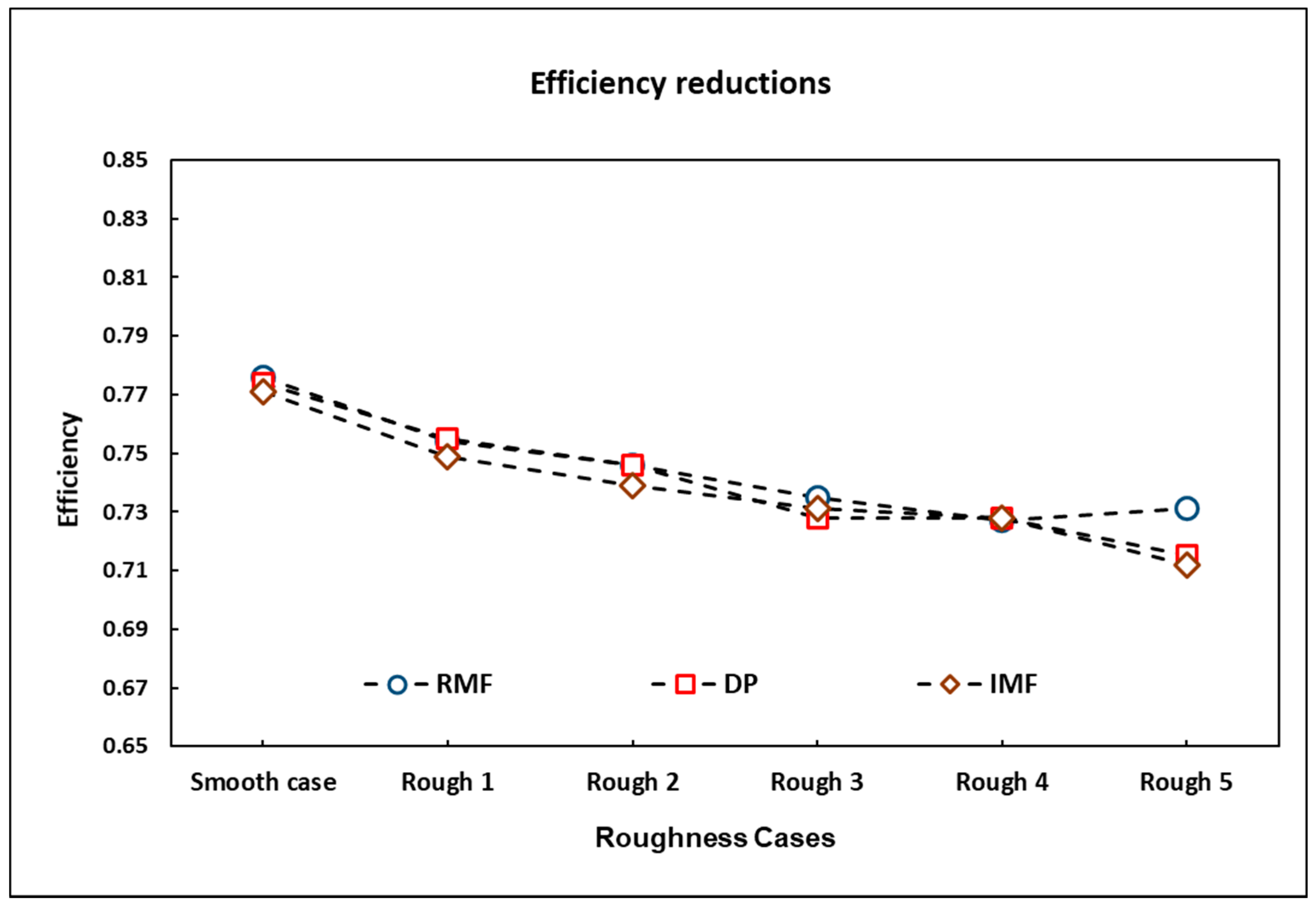
  • The increase in surface roughness of the first two stages of the LPC results in a quantifiable reduction in the performance variables of the research engine studied. The examined performance variables, isentropic efficiency, LPC PR, NDMF, TET, SFC, and overall PR exhibited, for the maximum blade surface degradation case, drops of 7.68%, 2.62% and 3.53%, rises of 1.14% and 0.69%, and a drop of 0.86%, respectively.
  • The maximum blade roughness results represent an extreme case, examined out of academic enquiry, since according to the literature, the SPE induced roughness level tends to stabilise independently of the erosion duration at around the 60 µm mark. The variation in the same parameters recorded above for this level of roughness, in terms of LPC PR, isentropic efficiency, NDMF, TET, SFC, and overall PR, corresponds to a drop of 1.85%, 5.92%, 2.72%, and increases of 0.81% and 0.51%, together with a drop of 0.63%, respectively.
  • The effect of increasing roughness on the LPC maps is characterised by the shift towards lower PR and NDMF values. The variation is more marked between the smooth and Rough 1 roughness regimes when compared to further roughness values. This observation has two aspects. Turbomachinery designers need to account for the operation of low pressure compressors used in propulsive applications to include the effects of a finite amount of roughness, which is an unavoidable consequence of their employment in eroding atmospheric environments. The second aspect relates to the physics of the erosion phenomenon, which limits the upper threshold of roughness of the blades and represents, therefore, a well-defined, worst-case scenario.
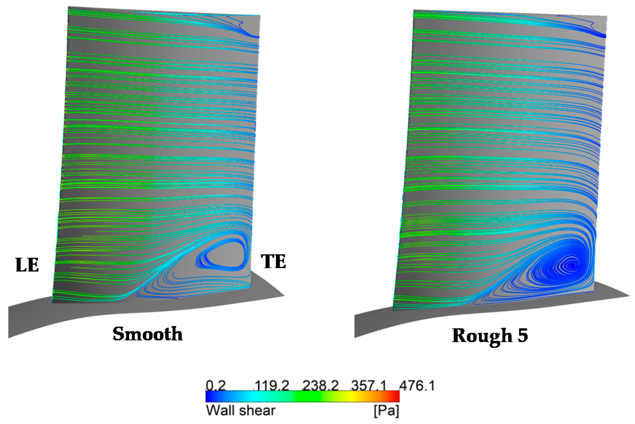
  • Although the various roughness levels examined were applied uniformly over the blades of the first two stages of the LPC, the SS region, as well as the early chordwise locations, exhibit the greatest variation, with reference to the smooth case in terms of chordwise C p coefficient. These regions are most effective at promoting the thickening of the local boundary layers, as evidenced through the total pressure distributions downstream of the blades as well as the pitchwise distribution of axial velocity.

Author Contributions

J.A. and J.A.T. conceived and designed the numerical models; J.A. performed the simulations; J.A.T. and J.A. analysed the simulation outcomes; J.A.T. contributed analysis tools; J.A. and J.A.T. wrote the paper. All authors have read and agreed to the published version of the manuscript.

Funding

This research received no external funding.

Institutional Review Board Statement

Not applicable.

Informed Consent Statement

Not applicable.

Acknowledgments

The authors of this article are grateful and acknowledge the help provided by their institutes. Also, the authors would like to express their gratitude to Natan Zawadzki for making his E3 inspired research engine model available as well as for many useful discussions during the elaboration of this paper.

Conflicts of Interest

The authors declare no conflict of interest.

Nomenclature

C p Total pressure loss coefficient
C r Log-layer constant
DP Design point
e a 21 Approximate relative error
e e x t 21 Extrapolated relative error
G C I F i n e 21 Fine-grid convergence index
h Cell size
HPC High pressure compressor
HPT High pressure turbine
kVon Karman constant
k s Equivalent sand-grain size (µm)
k s + Modified sand-grain roughness (µm)
LE Leading edge of the blade
LPC Low pressure compressor
LPT Low pressure turbine
( m ˙ ) Mass flow rate (kg/s)
M i n Mass flow at inlet (kg/s)
NDMFNon-dimensional mass flow
N 1, N 2, N 3 Total number of cells
P s Static pressure (Pa)
P 01 Total pressure (Pa)
PR Pressure ratio
PS Pressure side
RANS Reynolds Averaged Navier Stokes
R a Mean roughness (µm)
R e Reynolds number
R e k Roughness Reynolds number
r 21 ,   r 32   Grid refinement factor
SF Scaling factor
S F P R Scaling factor of the PR
S F N D M F Scaling factor of the NDMF
S F η i s Scaling factor of the isentropic efficiency
SFC Specific fuel consumption (g/kN.s)
SS Suction side
TE Trailing edge of the blade
TET Turbine entry temperature (K)
T 01 Total temperature (K)
U t Velocity parallel to the wall (m/s)
u + Dimensionless velocity
u τ Friction velocity (m/s)
u τ ˜ Modified friction velocity (m/s)
vKinematic viscosity (N.s/m2)
W 1 Relative inlet velocity (m/s)
y + Dimensionless distance from the wall
y + ˜ Modified dimensionless distance from the wall
Greek letters
ρDensity (kg/m3)
τ w Wall shear stress (Pa)
η i s Isentropic efficiency
Δ V i Cells volume (m3)
1 ,   2 ,   3 Pressure ratio (PR) values
e x t 21 Extrapolated value

References

  1. Szwaba, R.; Kaczynski, P.; Doerffer, P. Roughness effect on shock wave boundary layer interaction area in compressor fan blades passage. Aerosp. Sci. Technol. 2019, 85, 171–179. [Google Scholar] [CrossRef]
  2. Smil, V. The two prime movers of globalization: History and impact of diesel engines and gas turbines. J. Glob. Hist. 2007, 2, 373–394. [Google Scholar] [CrossRef] [Green Version]
  3. Alsayegh, A.; Ali, N. Gas turbine intercoolers: Introducing nanofluids—A mini-review. Processes 2020, 8, 1572. [Google Scholar] [CrossRef]
  4. Hu, J.; Wang, R.; Huang, D. Improvements of performance and stability of a single-stage transonic axial compressor using a combined flow control approach. Aerosp. Sci. Technol. 2019, 86, 283–295. [Google Scholar] [CrossRef]
  5. Alqallaf, J.; Ali, N.; Teixeira, J.A.; Addali, A. Solid particle erosion behaviour and protective coatings for gas turbine compressor blades-A review. Processes 2020, 8, 984. [Google Scholar] [CrossRef]
  6. Diakunchak, I.S. Performance deterioration in industrial gas turbines. Proc. ASME Turbo Expo. 1991, 4, 161–168. [Google Scholar]
  7. Brun, K.; Kurz, R.; Simmons, H.R. Aerodynamic instability and life-limiting effects of inlet and interstage water injection into gas turbines. J. Eng. Gas Turbines Power 2006, 128, 617–625. [Google Scholar] [CrossRef]
  8. Liu, C.; Cao, Y.; Ding, S.; Zhang, W. Effects of blade surface roughness on compressor performance and tonal noise emission in a marine diesel engine turbocharger. Proc. Inst. Mech. Eng. Part D J. Automob. Eng. 2020, 234, 3476–3490. [Google Scholar] [CrossRef]
  9. Ali, N.; Teixeira, J.A.; Addali, A.; Al-Zubi, F.; Shaban, E.; Behbehani, I. The effect of aluminium nanocoating and water pH value on the wettability behavior of an aluminium surface. Appl. Surf. Sci. 2018, 443, 24–30. [Google Scholar] [CrossRef] [Green Version]
  10. Ali, N.; Teixeira, J.A.; Addali, A.; Saeed, M.; Al-Zubi, F.; Sedaghat, A.; Bahzad, H. Deposition of stainless steel thin films: An electron beam physical vapour deposition approach. Materials 2019, 12, 571. [Google Scholar] [CrossRef] [Green Version]
  11. Ali, N.; Teixeira, J.A.; Addali, A. Effect of water temperature, ph value, and film thickness on the wettability behaviour of copper surfaces coated with copper using eb-pvd technique. J. Nano Res. 2019, 60, 124–141. [Google Scholar] [CrossRef]
  12. Burberi, C.; Michelassi, V.; Scotti Del Greco, A.; Lorusso, S.; Tapinassi, L.; Marconcini, M.; Pacciani, R. Validation of steady and unsteady CFD strategies in the design of axial compressors for gas turbine engines. Aerosp. Sci. Technol. 2020, 107, 106307. [Google Scholar] [CrossRef]
  13. Sun, S.; Wang, S.; Zhang, L.; Ji, L. Design and performance analysis of a two-stage transonic low-reaction counter-rotating aspirated fan/compressor with inlet counter-swirl. Aerosp. Sci. Technol. 2021, 111, 106519. [Google Scholar] [CrossRef]
  14. Kubacki, S.; Simoni, D.; Lengani, D.; Dick, E. An Extended Version of an Algebraic Intermittency Model for Prediction of Separation-Induced Transition at Elevated Free-Stream Turbulence Level. Int. J. Turbomach. Propuls. Power 2020, 5, 28. [Google Scholar] [CrossRef]
  15. Denton, J.D. Loss Mechanisms in Turbomachines; American Society of Mechanical Engineers: New York, NY, USA, 1993; Volume 78897, pp. 1–40. [Google Scholar]
  16. Hobson, G.V.; Millsaps, K.T.; Song, S.; Millsaps, K. Effects of Reynolds Number and Surface Roughness Magnitude and Location on Compressor Cascade Performance. J. Turbomach. 2012, 134, 051013. [Google Scholar]
  17. Melino, F.; Morini, M.; Peretto, A.; Pinelli, M.; Spina, P.R. Compressor fouling modeling: Relationship between computational roughness and gas turbine operation time. J. Eng. Gas Turbines Power 2012, 134, 052401. [Google Scholar] [CrossRef]
  18. Seehausen, H.; Gilge, P.; Kellersmann, A.; Friedrichs, J.; Herbst, F. Numerical Study of Stage Roughness Variations in a High Pressure Compressor. Int. J. Gas Turbine Propuls. Power Syst. 2020, 11, 16–25. [Google Scholar] [CrossRef]
  19. Pan, T.; Wu, W.; Li, Q. Effect of casing treatment to switch the type of instability inception in a high-speed axial compressor. Aerosp. Sci. Technol. 2021, 115, 106801. [Google Scholar]
  20. Hamed, A.; Tabakoff, W.; Wenglarz, R. Erosion and deposition in turbomachinery. J. Propuls. Power 2006, 22, 350–360. [Google Scholar] [CrossRef] [Green Version]
  21. Bammert, K.; Woelk, U.G. Influence of the Blading Surface Roughness on the Aerodynamic Behavior and Characteristic of an Axial Compressor. ASME Pap. 1979, 102, 283–287. [Google Scholar] [CrossRef]
  22. Zhihui, L.; Yanming, L. Optimization of rough transonic axial compressor. Aerosp. Sci. Technol. 2018, 78, 12–25. [Google Scholar]
  23. El-Sayed, A. Aircraft Propulsion And Gas Turbine Engines, 2nd ed.; Taylor & Francis Group: London, UK, 2017. [Google Scholar]
  24. Wang, M.; Yang, C.; Li, Z.; Zhao, S.; Zhang, Y.; Lu, X. Effects of surface roughness on the aerodynamic performance of a high subsonic compressor airfoil at low Reynolds number. Chin. J. Aeronaut. 2020, 34, 1–11. [Google Scholar] [CrossRef]
  25. Back, S.C.; Sohn, J.H.; Song, S.J. Impact of surface roughness on compressor cascade performance. J. Fluids Eng. Trans. ASME 2010, 132, 0645021–0645026. [Google Scholar] [CrossRef]
  26. Sun, H.O.; Ma, J.; Wang, Z.; Cao, L. The research on compressor performance degradation caused by surface roughness enlargement due to corrosion in marine environments. Proc. ASME Turbo Expo. 2019, 1, V001T25A003. [Google Scholar]
  27. Gray, D.; Et, A. NASA: Energy Efficient Engine Preliminary Design and Integration Studies Report; NASA: Hampton, VA, USA, 1978.
  28. Michael, C.J.; Halle, J.E. NASA: Energy Efficient Engine Low-Pressure Component Test Hardware Detailed Design Report; NASA: Hampton, VA, USA, 1981.
  29. Halle, J.; Michael, C.J. NASA: Energy Efficient Engine Fan Component Detailed Design Report; NASA: Hampton, VA, USA, 1981.
  30. Liu, Z.; Zhao, Y.; Chen, S.; Yan, C.; Cai, F. Predicting distributed roughness induced transition with a four-equation laminar kinetic energy transition model. Aerosp. Sci. Technol. 2020, 99, 105736. [Google Scholar] [CrossRef]
  31. ANSYS. ANSYS CFX-Solver Theory Guide; ANSYS: Canonsburg, PA, USA, 2016; pp. 1–350. [Google Scholar]
  32. Saidi, N.; Cerdoun, M.; Khalfallah, S.; Belmrabet, T. Numerical investigation of the surface roughness effects on the subsonic flow around a circular cone-cylinder. Aerosp. Sci. Technol. 2020, 107, 106271. [Google Scholar] [CrossRef]
  33. Launder, B.; Spalding, D. The Numerical Computation of Turbulent flows. Comput. Methods Appl. Mech. Eng. 1973, 3, 269–289. [Google Scholar] [CrossRef]
  34. Yang, L.; Zhou, J.; Fan, S.; Zheng, Q.; Zhang, H. Method and numerical simulation for evaluating the effects of water film on the performance of low-speed axial compressor. Aerosp. Sci. Technol. 2019, 84, 306–317. [Google Scholar] [CrossRef]
  35. Liu, C.; Shi, Y.; Cao, Y. Numerical study of effects of blade fouling on compressor performance and tonal noise emission. Aiaa Aviat. Forum 2020, 2699, 1–14. [Google Scholar]
  36. Li, Z.; Liu, Y. Effect of end-wall roughness on performance of transonic axial compressor. Proc. Inst. Mech. Eng. Part G J. Aerosp. Eng. 2017, 231, 1213–1224. [Google Scholar] [CrossRef]
  37. Syverud, E.; Bakken, L.E. The Impact of Surface Roughness on Axial Compressor Performance Deterioration. ASME Turbo Expo Power Land Sea Air 2006, 42401, 491–501. [Google Scholar]
  38. Aldi, N.; Morini, M.; Pinelli, M.; Spina, P.R.; Suman, A.; Venturini, M. Performance evaluation of nonuniformly fouled axial compressor stages by means of computational fluid dynamics analyses. J. Turbomach. 2014, 136, 1–11. [Google Scholar] [CrossRef]
  39. Zaita, A.V.; Butey, G.; Karlsons, G. Performance deterioration modeling in aircraft gas turbine engines. Proc. ASME Turbo Expo. 1998, 120, 4. [Google Scholar] [CrossRef]
  40. Celik, I.B.; Ghia, U.; Roache, P.J.; Freitas, C.J.; Coleman, H.; Raad, P.E. Procedure for estimation and reporting of uncertainty due to discretization in CFD applications. J. Fluids Eng. Trans. ASME 2008, 130, 0780011–0780014. [Google Scholar]
  41. Boyce, M.P. Principles Of Operation And Performance Estimation Of Centrifugal Compressors. In Proceedings of the 22nd Turbomachinery Symposium, College Station, TX, USA, 14–16 September 1993; pp. 161–178. [Google Scholar]
  42. Boyce, M.P. Gas Turbine Engineering Handbook, 2nd ed.; Gulf Professional Publishing: Oxford, UK, 2002; Volume 134. [Google Scholar]
  43. Zhang, Q.; Ligrani, P.M. Aerodynamic losses of a cambered turbine vane: Influences of surface roughness and freestream turbulence intensity. J. Turbomach. 2006, 128, 536–546. [Google Scholar] [CrossRef]
  44. Suder, K.L.; Chima, R.V.; Strazisar, A.J.; Roberts, W.B. The Effect of Adding Roughness and Thickness to a Transonic Axial Compressor Rotor. In Proceedings of the 39th International Gas Turbine and Aeroengine Congress and Exposition sponsored by the American Society of Mechanical Engineers, The Hague, The Netherlands, 13–16 June 1994; pp. 491–505. [Google Scholar]
  45. Sun, J.; Ottavy, X.; Liu, Y.; Lu, L. Corner separation control by optimizing blade end slots in a linear compressor cascade. Aerosp. Sci. Technol. 2021, 114, 106737. [Google Scholar] [CrossRef]
  46. De Giorgi, M.G.; Quarta, M. Hybrid MultiGene Genetic Programmin—Artificial neural networks approach for dynamic performance prediction of an aeroengine. Aerosp. Sci. Technol. 2020, 103, 105902. [Google Scholar] [CrossRef]
  47. Zhang, J.; Tang, H.; Chen, M. Robust design of an adaptive cycle engine performance under component performance uncertainty. Aerosp. Sci. Technol. 2021, 113, 106704. [Google Scholar] [CrossRef]
  48. Gallar, L.; Volpe, V.; Salussolia, M.; Pachidis, V.; Jackson, A. Thermodynamic gas model effect on gas turbine performance simulations. J. Propuls. Power 2012, 28, 719–727. [Google Scholar] [CrossRef]
  49. Suresh, S.; Nikolaidis, T.; Pilidis, P. TURBOMATCH-webengine—A web based gas turbine engine performance analysis tool. ASME Turbo Expo. 2013, 55188, 1–8. [Google Scholar]
  50. Nind, A.; Sethi, V.; Sampath, S. Towards the Development of A Technoeconomic, Environmental Risk Analysis for an Aircraft Operator, Awatef Hamed; Faculty Work and Research, College of Engineering and Applied Science: Cincinnati, OH, USA, 2015. [Google Scholar]
  51. Igie, U.; Abbondanza, M.; Szymański, A.; Nikolaidis, T. Impact of compressed air energy storage demands on gas turbine performance. Proc. Inst. Mech. Eng. Part A J. Power Energy 2020. [Google Scholar] [CrossRef] [Green Version]
  52. Meher-Homji, C.; Bromley, A. Gas Turbine Axial Compressor Fouling and Washing. Turbomach. Symp. 2004, 163–191. [Google Scholar] [CrossRef]
Figure 1. (a) Meridional view of the research engine components modelled, (b) computational domain, and (c) blading of IGV and first two booster stages.
Aerospace 08 00330 g001aAerospace 08 00330 g001b
Figure 2. (a) IGV, R2, and S2 grids; (b) Surface mesh on the hub and details of the LE and TE.
Aerospace 08 00330 g002aAerospace 08 00330 g002b
Figure 3. Computational domain and location of boundary conditions.
Aerospace 08 00330 g003
Figure 4. Comparison between the design calculation and the CFD points of the fan map at 100% and 90% speed-lines.
Aerospace 08 00330 g004
Figure 5. Variation of mass flow and NDMF with roughness at three operating points, 100% speed-line effect of roughness variation on pressure ratio and efficiency.
Aerospace 08 00330 g005
Figure 6. Pressure ratio reductions of the compressor at 100% design speed.
Aerospace 08 00330 g006
Figure 7. Efficiency reductions of the compressor at 100% design speed.
Aerospace 08 00330 g007
Figure 8. Effect of increasing surface roughness on the wall shear stress on the SS of the IGV.
Aerospace 08 00330 g008
Figure 9. Effect of increasing surface roughness on the wall shear stress of the SS of IGV (50% span).
Aerospace 08 00330 g009
Figure 10. Mach number distribution of compressor component at 50% spanwise, where (top) shows the smooth case and (bottom) illustrates the Rough 5 case.
Aerospace 08 00330 g010
Figure 11. Variation in total pressure rise in the booster with roughness.
Aerospace 08 00330 g011
Figure 12. Total pressure distribution at the exit of the IGV and the R3 for the smooth and Rough 5 cases and the difference between these two.
Aerospace 08 00330 g012
Figure 13. Distribution of axial velocity against non-dimensional pitch for the R2 and S2 at midspan.
Aerospace 08 00330 g013
Figure 14. Blade loading for five roughened cases ( C p vs. non-dimensional chord) for IGV, R2, S2, R3, and S3.
Aerospace 08 00330 g014
Figure 15. Turbomatch model of the research engine with station numbering.
Aerospace 08 00330 g015
Figure 16. Turbomatch results and theoretical design data for the E3 engine.
Aerospace 08 00330 g016
Figure 17. Compressor map of the 2-stages booster (PR).
Aerospace 08 00330 g017
Figure 18. Compressor map of the 2-stage booster (isentropic efficiency).
Aerospace 08 00330 g018
Figure 19. Performance variation of selected components against the roughened conditions for three operating points, 100% speed-line.
Aerospace 08 00330 g019
Table 1. Equivalent sand-grain size and the mean roughness values of the LPC blade surfaces.
Numberks (µm)Ra (µm)
Smooth case--
Rough 1152.419
Rough 2304.838
Rough 3457.258
Rough 4609.677
Rough 515024.193
Table 2. Fan, bypass, and low pressure compressor (LPC) design parameters. Reprinted with permission from ref. [27,28,29]. Copyright 2013 NASA Technical Report Server (NTRS).
ItemsUnitValue
Fan pressure ratio-1.74
Number of fan blades (R1)-24
R1 tip clearancemm1.39
Number of exit guide vanes (EGV) blades-29
Number of inlet guide vanes (IGV) blades-76
Number of second rotor blades (R2)-82
R2 tip clearancemm0.97
Number of stator blades (S2)-102
Number of third rotor blades (R3)-88
R3 tip clearancemm0.86
Number of third stator blades (S3)-110
Mass flow rate ( m ˙ ) (engine) (100% speed-line)kg/s623.73
mass flow rate (LPC) (100% speed-line)kg/s83.05
LPC pressure ratio (PR) (for the four stages)-1.77
LPC PR (for the first two stages)-1.336
Rotational speed for 100% speed-liner/min4215
Table 3. Results of the grid and turbulence model sensitivity study for R2.
ParametersCoarse MeshMedium MeshFine Mesh
Number of nodes
(all components)
3.1 M4 M8 M
Polytropic efficiency
(SST turbulence model)
0.950.960.96
Simulation time
(SST turbulence model)
4 h and 53 min6 h and 35 min9 h and 50 min
Table 4. Number of nodes in medium mesh for each of the blade rows.
ComponentsNumber of Nodes
Fan1.6 M
Bypass417 k
IGV387 k
R2389 k
S2357 k
R3402 k
S3478 k
Table 5. Outcomes of the discretization error.
Components∅ = PR (with Monotonic Convergence)
N1, N2, N33,106,608, 3,987,820, 7,963,228
r 21 0.92
r 32 0.80
1 1.28
2 1.30
3 1.31
P3.02
e x t 21 1.33
e a 21 0.63%
e e x t 21 2.78%
G C I f i n e 21 3.5%
Table 6. Comparison of the numerical results and the design calculation’s values.
ParameterCFD ResultsReferenceDeviation (%)
m ˙ (kg/s)84.783.11.8
PR (2-stage booster)1.301.342.9
T 2 at stage 2 exit (K)344.2333.03.2
ηis (2-stage booster)0.790.823.6
Table 7. Reduction in PR, NDMF, and isentropic efficiency of the first two booster stages by reference to the smooth case.
CaseReduction
PRNDMF η i s  
Smooth---
Rough 10.9920.9870.974
Rough 20.9910.9810.962
Rough 30.9810.9730.939
Rough 40.9820.9720.940
Rough 50.9730.9640.9231
Table 8. Effect of surface roughness on the performance variables of the research engine.
CaseDeviation (%)(Δ)
EPRSFCTET (K)
Smooth---
Rough 1−0.275+0.204+5.8
Rough 2−0.426+0.292+8.6
Rough 3−0.633+0.476+13.7
Rough 4−0.626+0.502+13.7
Rough 5−0.862+0.687+19.1
Publisher’s Note: MDPI stays neutral with regard to jurisdictional claims in published maps and institutional affiliations.

