A Hybridized Discontinuous Galerkin Solver for High-Speed Compressible Flow

Abstract

We present a high-order consistent compressible flow solver, based on a hybridized discontinuous Galerkin (HDG) discretization, for applications covering subsonic to hypersonic flow. In the context of high-order discretization, this broad range of applications presents unique difficulty, especially at the high-Mach number end. For instance, if a high-order discretization is to efficiently resolve shock and shear layers, it is imperative to use adaptive methods. Furthermore, high-Enthalpy flow requires non-trivial physical modeling. The aim of the present paper is to present the key enabling technologies. We discuss efficient discretization methods, including anisotropic metric-based adaptation, as well as the implementation of flexible modeling using object-oriented programming and algorithmic differentiation. We present initial verification and validation test cases focusing on external aerodynamics.

1. Introduction

Compressible flow simulation has long been dominated by at most second order consistent methods. Prime examples are finite volume schemes and stabilized finite element schemes [1,2,3,4,5,6,7,8]. Higher order consistent methods promise superior resolution at reduced number of degrees-of-freedom (DoF), provided the solution is (locally) smooth enough [9]. In compressible flow, however, flow features such as shock waves can compromise local solution regularity. Moreover, besides shock waves, other strongly anisotropic features are usually present. Examples include boundary and shear layers. To allow efficient resolution of these features, while taking advantage of superior resolution on coarse elements, whenever the flow is smooth, a good high-order methodology ought to be adaptive, preferably using anisotropic adaptation. Furthermore, computations are often carried out primarily with the aim to compute a few solution-dependent functionals very accurately. Examples, such as force or heat transfer coefficients, readily come to mind. This suggests goal-oriented adaptation, which may be implemented via adjoint methods [10].

For a while now, metric-based adaptation methods have been used in compressible flow simulation [11,12,13,14]. A convenient formalism for such methods is the continuous mesh framework [15,16]. However, the formulation for high-order discretization, using piecewise polynomial approximation methods, has been relatively recent [17,18]. In previous work, we proposed a high-order method using analytical optimization of the continuous mesh model [18,19], including hp-adaptation [20] and goal-oriented adaptation [21,22]. The main advantage is that the procedure is entirely free of parameters, using only a constraint given by the overall mesh-complexity. Demonstrating the fidelity of our high-order continuous mesh method with respect to high-Mach number flow is the first aim of the present paper.

Secondly, for the wide range of applications and flow conditions envisioned here, one has to consider a range of physical models. In our implementation we use the library Mutation++ [23] to provide a flexible interface to thermodynamic closure equations and transport coefficients. We present an efficient implementation framework, based on object-oriented programming and class-based templates.

Finally, the flexible approach to modeling has implications for the overall solution strategy applied to the nonlinear discretized equations. Compressible flow discretization usually leads to stiff problems. This is even more pronounced for high-order discretization methods on very anisotropic grids. Under these circumstances, fully coupled implicit methods are attractive. For instance, Newton–Raphson methods offer asymptotic quadratic convergence, provided a very accurate differentiation of the residual function is available. This is a complication when the goal is to support easy implementation of different physical models, as it requires not only implementation of the physical model, but also its differentiation with respect to the state. We use algorithmic differentiation to facilitate the embedding of different physical models into our solver framework.

The idea of using higher order methods to simulate compressible flow is not new [24,25], and indeed there are publicly available tools [26,27]. Moreover, there is recent work with partially overlapping scope [28,29,30]. In particular, Nguyen et al. developed a high-order HDG solver and used it to simulate hypersonic flow, using a single-species, perfect gas model [30]. However, at the intersection of (1) high-order methods, (2) high-Mach-number flow, (3) flexible, non-trivial physical modeling, (4) anisotropic adaptation, and (5) fast solver convergence, there is a dearth of existing tools.

In summary, the purpose of this paper is to present a high-order HDG solver for high-Mach-number flows addressing the above aspects. Our solver originates from the work first presented in [31]. The overall implementation strategy is designed to support a wide range of applications and flexible modeling, while keeping the solver components (adaptation, implicit solution methods, etc.) intact without extensive programming efforts. The paper is organized as follows: In Section 2, we briefly review the governing equations. Next, in Section 3 and Section 4, we discuss the discretization and adaptation methods used in this work, while Section 5 discusses our implementation strategy. Finally, in Section 6 we present numerical results.

2. Governing Equations

Our computational approach is designed to solve balance laws of the following type:

$$\frac{\partial \mathit{u}}{\partial t}+\sum _{i=1}^d\frac{\partial {\mathit{f}}_i(\mathit{u},\nabla \mathit{u})}{\partial x_i}=\mathit{S}(\mathit{u},\nabla \mathit{u}).$$

(1)

where $(1,\dots ,d)=:\mathit{f}$ is the flux vector, and $\mathit{S}$ is a source term. In the present paper, we focus on steady compressible flow problems. We consider models for a homogeneous mixture of ideal gases with frozen chemistry, as well as models for a mixture in chemical non-equilibrium.

For a gas composed of $N_s$ molecular species, the state vector of conserved variables is written as

$$\mathit{u}=\left(\begin{array}{c}\mathit{\rho }\\ \rho \mathit{v}\\ E\end{array}\right),$$

(2)

where $\mathit{\rho }={({\rho }_1,\dots ,{\rho }_{N_s})}^T$ is the vector of species densities, and $\rho ={\sum }_{i=1}^{N_s}{\rho }_i$ is the total density. The bulk fluid velocity vector and total energy are denoted by $\mathit{v}={(v_1,\dots ,v_d)}^T$, and E, respectively. In the absence of chemical reactions (frozen flow), we may treat the gas as a homogenous mixture. In this case, we may set $N_s=1$, and only one mass equation is solved. (The same is true for flows in local thermodynamic equilibrium (LTE), where chemical reactions are assumed to be fast enough, such that the equilibrium mixture is locally achieved and provided that the elemental composition is frozen. However, we do not consider LTE models in this work.)

We write $\mathit{f}={\mathit{f}}_c-{\mathit{f}}_v$, where ${\mathit{f}}_c$ and ${\mathit{f}}_v$, are the convective and diffusive flux, respectively. Together with the source term $\mathit{S}$, they are given by

$${\mathit{f}}^c=\left(\begin{array}{c}\rho {\mathit{v}}^T\\ \rho \mathit{v}{\mathit{v}}^T+p{\mathit{I}}_d\\ \left(E+p\right){\mathit{v}}^T\end{array}\right),{\mathit{f}}^v=\left(\begin{array}{c}-\mathit{J}\\ \mathit{\tau }\\ {\mathit{v}}^T\mathit{\tau }-{\mathit{q}}^T\end{array}\right),\mathit{S}=\left(\begin{array}{c}\dot{\omega }\\ \mathbf{0}\\ 0\end{array}\right).$$

(3)

Here, p is the pressure. Moreover, $\mathit{\tau }={\left({\mathit{\tau }}_{ij}\right)}_{i,j=1,\dots ,d}$ is the viscous stress tensor, $\mathit{q}={(q_1,\dots ,q_d)}^T$ is the heat flux vector, $\mathit{J}={\left(J_{ij}\right)}_{i=1,\dots N_s,j=1,\dots ,d}$ is the species diffusion flux, and $\dot{\omega }={({\dot{\omega }}_1,\dots ,{\dot{\omega }}_{N_s})}^T$ is the vector of reaction rates. Models for these quantities are discussed below. For simple fluid models with frozen chemistry and negligible species diffusion, $N_s=1$, $\mathit{J}=\mathbf{0}$, and $\dot{\omega }=\mathbf{0}$. If, furthermore, the flow is considered inviscid, $\mathit{\tau }=\mathbf{0}$ and $\mathit{q}=\mathbf{0}$.

Closure Equations, Constitutive Models, and Transport Coefficients

We assume that the gas mixture is thermally perfect (although not necessarily calorically perfect). This assumption is often made in high-enthalpy hypersonic applications where the pressure is not too high [32]. Thus, each species satisfies the ideal gas law for the partial pressure $p_i$, and the mixture satisfies Dalton’s law,

$$p=\sum _{i=1}^{N_s}{p}_i=\sum _{i=1}^{N_s}{\rho }_i{R}_{i}T,$$

(4)

where $R_i$ is the specific gas constant of species i. Under the above assumptions, we have $R_i=c_{p,i}-c_{v,i}$, where $c_{v,i}=c_{v,i}\left(T\right)$ and $c_{p,i}=c_{p,i}\left(T\right)$ are the specific heat capacities at constant volume and pressure, respectively. The thermal energy and enthalpy of each species are solely determined by the temperature [33]:

$$e_i={\int }_{T_0}^T{c}_{v,i}\left(T\right)dT+e_{0,i},h_i={\int }_{T_0}^T{c}_{p,i}\left(T\right)dT+h_{0,i}.$$

(5)

Under the present modeling assumptions, we obtain the bulk thermal energy and enthalpy as weighted by the mixture composition:

$$e=\sum _{i=1}^{N_s}{Y}_i{e}_i,h=\sum _{i=1}^{N_s}{Y}_i{h}_i.$$

(6)

Here, $Y_i={\rho }_i/\rho$ is the mass fraction of species i. For frozen chemistry, we may use the effective gas constant R, given by ${\sum }_{i=1}^{N_s}{Y}_i{R}_i$, where $Y_i$ is assumed constant, to compute

$$p=\rho RT.$$

(7)

Simpler models, which may be used in external aerodynamics under subsonic or moderately supersonic free stream conditions, regard the mixture as a both thermally and calorically perfect gas. Under these assumptions we may write the equation of state as

$$p=(\gamma -1)\rho e=(\gamma -1)\left(E-\frac{1}{2}\rho \mathit{v}·\mathit{v}\right),$$

(8)

where $\gamma$ is the (constant) ratio of specific heats.

When considering Newtonian viscous flow, the stress tensor is given by

$$\mathit{\tau }=\mu (\nabla \mathit{v}+{(\nabla \mathit{v})}^T-\frac{2}{3}(\nabla ·\mathit{v}){\mathit{I}}_d),$$

where for simplicity, we set the bulk viscosity to zero. For moderate temperatures, one may use Sutherland’s law [34] to compute the viscosity $\mu =\mu \left(T\right)$ as

$$\mu =\frac{C_1{T}^{3/2}}{C_2+T},$$

(9)

with $C_1=1.458·{10}^{-6}\frac{\mathrm{kg}}{\mathrm{ms}\sqrt{\mathrm{K}}}$ and $C_2=110.4\mathrm{K}$ for an air mixture. For higher temperatures, the library Mutation++ may be used to compute the viscosity from the current local state.

As mentioned above, we distinguish between simple fluid models with frozen chemistry, characterized by constant mass fractions, and more general gas mixtures. For the former, recall that only one mass equation is solved. For the latter, we model species diffusion using Fick’s law with averaged species diffusion coefficients [35,36],

$${\mathit{J}}_i=-\rho D_i\nabla Y_i+Y_i\sum _{j=1}^{N_s}\rho D_j\nabla Y_j.$$

(10)

Thermal and baro-diffusion effects were neglected here. Please note that the second term ensures zero net diffusion flux, when summed over all species. The averaged species diffusion coefficients $D_i$ are obtained directly from Mutation++ from the binary diffusion coefficients of the gas mixture. More accurate diffusion models, using multicomponent diffusion coefficients, are available in Mutation++, but have not been used here.

We model the heat flux using Fourier’s law and energy transfer due to species diffusion (neglecting thermal diffusion induced by species diffusion) [36]:

$$\mathbf{q}=\sum _{i=1}^{N_s}{h}_i{\mathbf{J}}_i-k\nabla T.$$

(11)

Here, k is the mixture thermal conductivity. For simple fluid models with $Y_i=const.$, only the second term is present. At moderate flow conditions, we may assume a constant Prandtl number, whence

$$k=\frac{\mu c_p}{\mathrm{Pr}}.$$

(12)

For example, $\mathrm{Pr}=0.72$ for air. At higher temperatures, this is no longer a good approximation, and we again use the library Mutation++ to compute the thermal conductivity k from the local state.

Finally, for flows in chemical non-equilibrium, the species source terms $\dot{\omega }$ must be considered. These represent the creation and destruction of the species through chemical reactions. Upon choosing a desired mixture model with a predefined set of $N_r$ elementary reactions, Mutation++ models the reaction rates using the Law of Mass Action, and provides the local net production rates for each species. The forward rate coefficients are computed based on Arrhenius’ law. The forward and backward rate coefficients are linked through the equilibrium constant, satisfying the second law of thermodynamics [37].

To summarize,

Table 1. Overview of models used in the present paper. Please note that the first two models solve only one mass Equation (with $\mathit{J}=\mathbf{0}$ and $\dot{\omega }=\mathbf{0}$).

	Model 1	Model 2	Model 3
	Perfect Gas	High-Enthalpy Frozen	High-Enthalpy Non-Equilibrium
Number of equations	$d+2$	$d+2$	$N_s+d+1$
Equation of state	Equation (8)	Equation (7)	Equation (4)
Viscosity	Equation (9)	Equation (9) or Mutation++	Mutation++
Thermal Conductivity	Equation (12)	Equation (12) or Mutation++	Mutation++
Species Diffusion	-	-	Mutation++
Production Rates	-	-	Mutation++

gives an overview of models used in the present work.

3. Numerical Discretization

3.1. Hybridized Discontinuous Galerkin Method

The governing equations presented in Section 2 are discretized using a hybridized discontinuous Galerkin (HDG) method. We only give a brief summary here. A more detailed overview of HDG schemes can be found elsewhere [38,39,40].

Let $\mathsf{\Omega }$ be the computational domain. For a given a triangulation ${\mathcal{T}}_h=\left\{\kappa \right\}$, and setting $m=N_s+d+1$ for the number of equations to be solved, we define the approximation spaces

$$\begin{array}{cc}\hfill V_h& :=\{\mathit{w}\in {\left(L^2\left(\mathsf{\Omega }\right)\right)}^m:\mathit{w}{|}_{\kappa }\in {\left(P^p\left(\kappa \right)\right)}^m,\forall \kappa \in {\mathcal{T}}_h\}\hfill \end{array}$$

(13)

$$\begin{array}{cc}\hfill {\mathsf{\Sigma }}_h& :=\{\zeta \in {\left(L^2\left(\mathsf{\Omega }\right)\right)}^{m\times d}:\zeta {|}_{\kappa }\in {\left(P^p\left(\kappa \right)\right)}^{m\times d},\forall \kappa \in {\mathcal{T}}_h\}\hfill \end{array}$$

(14)

$$\begin{array}{cc}\hfill {\mathsf{\Lambda }}_h& :=\{\nu \in {\left(L^2\left({\mathcal{E}}_h^0\right)\right)}^m:\nu {|}_e\in {\left(P^p\left(e\right)\right)}^m,\forall e\in {\mathcal{E}}_h^0\}.\hfill \end{array}$$

(15)

Here ${\mathcal{E}}_h^0$ denotes the set of interior edges, and $P^p$ denotes the space of polynomials with total degree at most p. Upon defining ${\mathbb{X}}_h:={\mathsf{\Sigma }}_h\times V_h\times {\mathsf{\Lambda }}_h$, the HDG discretization of the steady-state version of the balance law (1) is given as the variational problem

$${\mathbf{x}}_h\in {\mathbb{X}}_h:N_h({\mathbf{x}}_h,\mathbf{y})=0,\forall \mathbf{y}\in {\mathbb{X}}_h.$$

(16)

Defining elementwise integration,

$$\begin{array}{cccc}\hfill {\int }_{{\mathcal{T}}_h}·dx& :=\sum _{\kappa \in {\mathcal{T}}_h}{\int }_{\kappa }·dx,\hfill & \hfill {\int }_{\partial {\mathcal{T}}_h^0}·ds& :=\sum _{\kappa \in {\mathcal{T}}_h}{\int }_{\partial \kappa \backslash {\mathcal{E}}_h^{\partial }}·ds,\hfill \end{array}$$

where ${\mathcal{E}}_h^{\partial }$ are the boundary edges, and setting ${\mathbf{x}}_h=({\sigma }_h,{\mathit{u}}_h,{\lambda }_h)$, $\mathbf{y}=(\zeta ,\mathit{w},\nu )$, we can write

$$\begin{array}{cc}\hfill N_h({\mathbf{x}}_h,\mathbf{y})={\int }_{{\mathcal{T}}_h}{\sigma }_h:\zeta dx+{\int }_{{\mathcal{T}}_h}({\mathit{u}}_h\otimes \nabla ):\zeta dx-{\int }_{\partial {\mathcal{T}}_h^0}{\lambda }_h\otimes \mathit{n}:\zeta ds-{\int }_{{\mathcal{E}}_h^{\partial }}{\widehat{\mathit{u}}}^b\otimes \mathit{n}:\zeta ds& \hfill \\ \hfill -{\int }_{{\mathcal{T}}_h}\mathit{f}({\mathit{u}}_h,{\sigma }_h\mathit{n}):\nabla \mathit{w}dx+{\int }_{\partial {\mathcal{T}}_h^0}\widehat{\mathit{f}}({\sigma }_h,{\mathit{u}}_h,{\lambda }_h;\mathit{n})·\mathit{w}ds+{\int }_{{\mathcal{E}}_h^{\partial }}{\widehat{\mathit{f}}}^b({\sigma }_h,{\mathit{u}}_h;\mathit{n})·\mathit{w}ds& \hfill \\ \hfill -{\int }_{{\mathcal{T}}_h}\mathit{S}({\mathit{u}}_h,{\sigma }_h)·\mathit{w}dx+{\int }_{{\mathcal{E}}_h^0}\left[\left[\widehat{\mathit{f}}({\sigma }_h,{\mathit{u}}_h,{\lambda }_h;\mathit{n})\right]\right]·\mathit{\nu }ds& .\hfill \end{array}$$

(17)

The numerical flux function is written as $\widehat{\mathit{f}}={\widehat{\mathit{f}}}_c-{\widehat{\mathit{f}}}_v$, where ${\widehat{\mathit{f}}}_c$ and ${\widehat{\mathit{f}}}_v$ are standard convective and viscous numerical fluxes, respectively. In the present work we use the Lax-Friedichs flux for the former, and the LDG flux for the latter. More precisely, let elements ${\kappa }^{+}$ and ${\kappa }^{-}$ be separated by edge $e\in {\mathcal{E}}_h^0$, Then we define the numerical fluxes such that

$$\begin{array}{cccc}\hfill {\widehat{\mathit{f}}}_c\equiv {\widehat{\mathit{f}}}_c^{\pm }& :=\mathit{f}\left({\lambda }_h\right)·{\mathit{n}}^{\pm }-{\alpha }_c\left({\lambda }_h-{\mathit{u}}_h^{\pm }\right)\hfill & \hfill & \mathrm{on}e\hfill \end{array}$$

(18)

$$\begin{array}{cccc}\hfill {\widehat{\mathit{f}}}_v\equiv {\widehat{\mathit{f}}}_v^{\pm }& :=\mathit{f}({\lambda }_h,{\sigma }_h^{\pm })·{\mathit{n}}^{\pm }-{\alpha }_v\left({\lambda }_h-{\mathit{u}}_h^{\pm }\right)\hfill & \hfill & \mathrm{on}e\hfill \end{array}$$

(19)

Here ${\mathit{n}}^{\pm }$ denotes the outward pointing normal on $\partial {\kappa }^{\pm }$, and ${\mathit{u}}_h^{\pm }$, ${\sigma }_h^{\pm }$ are the limits of the respective functions approaching the iterface from ${\kappa }^{\pm }$. (Please note that ${\lambda }_h$ is single-valued by definition.) The jump of the total flux on e then reads $\left[\left[\widehat{\mathit{f}}\right]\right]={\widehat{\mathit{f}}}^{+}{\mathit{n}}^{+}+{\widehat{\mathit{f}}}^{-}{\mathit{n}}^{-}$. Again, it ought to be noted that the numerical flux functions are not by definition conservative. Instead, the last term in (17) enforces conservation as a constraint [39,40,41]. Finally, the boundary fluxes ${\widehat{\mathit{u}}}^b$ and ${\widehat{\mathit{f}}}^b({\mathit{u}}_h,{\sigma }_h;\mathit{n})$ are assumed to be consistent with the boundary conditions [42].

To avoid oscillations near discontinuities, the discretization can be augmented with a shock-capturing term. At present, we use a classic method based on artificial viscosity [43,44]. We define

$$N_h^{SC}({\mathbf{x}}_h,\mathbf{y}):={\int }_{{\mathcal{T}}_h}ϵ\left({\mathit{u}}_h\right){\sigma }_h:\nabla \mathit{w}dx.$$

(20)

The artificial diffusion coefficient is computed as a function of the solution ${\mathit{u}}_h$, such that

$$ϵ\left({\mathit{u}}_h\right){|}_{\kappa }:=\frac{{ϵ}_0{(h_{\kappa }/p_{\kappa })}^{2-\beta }}{\left|\kappa \right|}{\int }_{\kappa }\sum _{i=1}^m|\nabla ·{\mathit{f}}_c\left({\mathit{u}}_h\right)|dx,\forall \kappa \in {\mathcal{T}}_h.$$

(21)

Here $h_{\kappa }$ is the diameter of $\kappa$, and $p_{\kappa }$ is the polynomial degree of approximation. The parameters ${ϵ}_0$ and $\beta$ can be used to tune the shock-capturing term. In the present work, we set $\beta =0$. The term (20) can be added to the semilinear form (17) to provide nonlinear stabilization. This approach is somewhat generic in the sense that it is not especially tuned to the physical model under consideration. It has proven successful for transonic and supersonic external aerodynamics. Below we show that the range of application extends to moderately hypersonic flow conditions, not exceeding $M_{\infty }\approx 8$. For higher Mach numbers more carefully tuned shock capturing may become necessary [30].

Equation (16) is solved using a Newton–Raphson method. Writing ${\mathbf{x}}_h^{n+1}={\mathbf{x}}_h^n+\delta {\mathbf{x}}_h^n$, the linearized global system is given in block-matrix form as

$$\left[\begin{array}{ccc}A& B& R\\ C& D& S\\ L& M& N\end{array}\right]\left[\begin{array}{c}\delta Q\\ \delta W\\ \delta \mathsf{\Lambda }\end{array}\right]=\left[\begin{array}{c}F\\ G\\ H\end{array}\right],$$

(22)

where the vector ${\left[\delta Q,\delta W,\delta \mathsf{\Lambda }\right]}^T$ contains the expansion coefficients of $\delta {\mathbf{x}}_h^n=(\delta {\sigma }_h$, $\delta {\mathit{u}}_h$, $\delta {\lambda }_h$) with respect to the chosen basis. The matrix on the left represents the Jacobian matrix of $N_h({\mathbf{x}}_h,\mathbf{y})$ as a function of these coefficients. In particular, the nonlinear contributions from flux functions, numerical flux functions, and boundary fluxes are often cumbersome to compute. Moreover, these elements change upon implementation of a new physical model. It is here that the algorithmic differentiation mentioned in the introduction is very useful. We come back to this issue in Section 5 below.

Taking the Schur complement, one obtains the hybridized system

$$\left(N-\left[\begin{array}{cc}L& M\end{array}\right]{\left[\begin{array}{cc}A& B\\ C& D\end{array}\right]}^{-1}\left[\begin{array}{c}R\\ S\end{array}\right]\right)\delta \mathsf{\Lambda }=H-\left[\begin{array}{cc}L& M\end{array}\right]{\left[\begin{array}{cc}A& B\\ C& D\end{array}\right]}^{-1}\left[\begin{array}{c}F\\ G\end{array}\right].$$

(23)

System (23) is solved at each Newton iteration using an iterative linear solver. This system is clearly algebraically equivalent to (22). Moreover, the structure of the HDG discretization makes its assembly economically feasible, as the sub-matrix to be inverted is block-diagonal. The system is globally coupled only in the degrees-of-freedom corresponding to ${\lambda }_h$. This remains true when the shock-capturing term (20) is added. In contrast, standard DG schemes, written in primal form (possibly upon locally eliminating the degrees-of-freedom Q, which can be done for all standard DG schmes [45]), lead to larger linear systems. This is increasingly so for higher polynomial degree p [44]. Indeed, HDG schemes were found to be competitive in terms of efficiency with continuous Galerkin schemes using static condensation [46].

3.2. Adjoint Equations

Let $J(\mathit{u},\nabla \mathit{u})$ be a solution-dependent functional, and let $J_h\left({\mathbf{x}}_h\right)$ be a consistent approximation, such that for $\mathbf{x}=(\mathit{u},\nabla \mathit{u},\mathit{u}{|}_{{\mathcal{E}}_h^0})$, $J_h\left(\mathbf{x}\right)=J(\mathit{u},\nabla \mathit{u})$. Adjoint methods can be used to provide a map to relate variations in the functional to the discrete residual. An approximation is given by the discrete adjoint method, where

$$J_h\left({\mathbf{x}}_h\right)-J(\mathit{u},\nabla \mathit{u})\approx N_h({\mathbf{x}}_h,{\mathbf{z}}_h),$$

(24)

provided that ${\mathbf{z}}_h\in {\widehat{\mathbb{X}}}_h\supset {\mathbb{X}}_h$ satisfies, for a fixed solution ${\mathbf{x}}_h\in {\mathbb{X}}_h$ of the primal problem,

$$N_h^{\prime }\left[{\mathbf{x}}_h\right](\mathbf{y},{\mathbf{z}}_h)=J^{\prime }\left[{\mathbf{x}}_h\right]\left(\mathbf{y}\right),\forall \mathbf{y}\in {\widehat{\mathbb{X}}}_h.$$

(25)

Please note that taking the adjoint solution from a superset ${\widehat{\mathbb{X}}}_h\supset {\mathbb{X}}_h$ is necessary to avoid an identically zero right-hand side in (24). The adjoint-based error estimate can be used to drive a goal-oriented adaptation process [47].

We proved in a previous publication that, with appropriate treatment of boundary conditions, the HDG discretization (17) is adjoint consistent [42,48]. It remains asymptotically adjoint consistent when the shock capturing term (20) is added. In other words, the discrete adjoint equations automatically give a consistent discretization of the adjoint PDE with appropriate boundary conditions. This is true for admissible functionals of the form

$$J(\mathit{u},\nabla \mathit{u})={\int }_{\partial \mathsf{\Omega }}\beta \otimes \mathit{n}:\mathit{f}(\mathit{u},\nabla \mathit{u})ds,$$

(26)

where $\beta$ is any $L^2$ function. For instance, at an adiabatic wall one has, by the definition of the fluxes and the boundary conditions,

$$\mathit{f}(\mathit{u},\nabla \mathit{u})·\mathit{n}=({\mathit{f}}_c\left(\mathit{u}\right)-{\mathit{f}}_v(\mathit{u},\nabla \mathit{u}))·\mathit{n}=\left(\begin{array}{c}0\\ p\mathit{n}\\ 0\end{array}\right)-\left(\begin{array}{c}0\\ \mathit{\tau }\mathit{n}\\ 0\end{array}\right).$$

(27)

Thus, compatible functionals include force coefficients. For non-adiabatic walls, heat transfer coefficients may also be used [42].

4. Adaptation

Metric-based methods have emerged as an interesting paradigm for mesh adaptation. The idea is to encode a desirable mesh in a tensor-valued mapping, yielding a one-parameter family of s.p.d. matrices, ${\left(\mathcal{M}\left(x\right)\right)}_{x\in \mathsf{\Omega }}$, where $\mathsf{\Omega }\subset {\mathbb{R}}^d$ is some computational domain. A metric-conforming mesh is a triangulation whose elements are (nearly) equilateral under the Riemannian metric induced by $\mathcal{M}$. This mapping is the continuous mesh [15]. In this section, we summarize our continuous mesh optimization, which we used in the computational studies below. More details can be found in [18,19,20,21,22].

4.1. Encoding a Mesh via Metric Tensors

Let ${\mathcal{T}}_h:=\left\{\kappa \right\}$ be a triangulation of $\mathsf{\Omega }$. For any non-degenerate simplex element, there is a unique symmetric positive definite matrix

$$\mathbb{M}=\left(\begin{array}{cc}{m}_{11}& m_{12}\\ m_{12}& m_{22}\end{array}\right)$$

(28)

such that,

$$\left|\right|{\mathit{e}}_i{\left|\right|}_{\mathbb{M}}^2={\mathit{e}}_i^T\mathbb{M}{\mathit{e}}_i=C,i=1,2,3,$$

(29)

where ${\mathit{e}}_i$ is an edge of the triangle, given as a vector of arbitrary orientation. In other words, the mesh element is equilateral in the norm $\left|\right|·{\left|\right|}_{\mathbb{M}}^{}$ induced by the metric $\mathbb{M}$, i.e.,

$${\left|\right|\mathit{x}\left|\right|}_{\mathbb{M}}^{}:=\sqrt{{\mathit{x}}^T\mathbb{M}\mathit{x}}.$$

We say the element is $unit$ with respect to $\mathbb{M}$. A straightforward geometric interpretation is shown in Figure 1: The mesh element is inscribed into the unit circle ${\left|\right|\mathit{x}\left|\right|}_{\mathbb{M}}^{}=1$ (i.e., an ellipse).

It will prove useful to characterize the metric by its eigenstructure, i.e., $\mathbb{M}=Q^T\mathsf{\Lambda }Q$, where

$$Q=\left(\begin{array}{cc}cos\theta & sin\theta \\ -sin\theta & cos\theta \end{array}\right)\mathsf{\Lambda }=\mathrm{diag}({\lambda }_1,{\lambda }_2)$$

(30)

Thus, $\mathbb{M}$ may be represented by the tuple $(d,\zeta ,\theta )$, where the angle $\theta$ defines the orientation of the eigenvectors in (30), and

$$\zeta :=\sqrt{\frac{{\lambda }_1}{{\lambda }_2}},d:=\sqrt{{\lambda }_1{\lambda }_2}$$

(31)

are the aspect ratio and mesh density, respectively. The latter definition is motivated by the relation

$$d=\frac{\alpha }{\left|\kappa \right|}$$

(32)

where the constant $\alpha$ depends only on the constant C in (29).

Given an element-wise metric, one may, using a suitable interpolation, generate a metric field ${\left(\mathcal{M}\left(x\right)\right)}_{x\in \mathsf{\Omega }}$, defined for any $x\in \mathsf{\Omega }$. Metric-based mesh generators can generate a discrete mesh, composed of elements which are unit with respect to a metric field, usually interpreted in a least-squares sense, such that one approximates the solution to the minimization problem

$${\mathcal{T}}_h^{\star }=\arg {\min }_{{\mathcal{T}}_h}\sum _{\mathit{e}\in {\mathcal{T}}_h}\left|{\left|\right|\mathit{e}\left|\right|}_{\mathcal{M}}^2-C\right|.$$

The length of a segment $\mathit{e}:={\mathit{x}}_2-{\mathit{x}}_1$ under the metric ${\left(\mathcal{M}\left(\mathit{x}\right)\right)}_{\mathit{x}\in \mathsf{\Omega }}$ is now interpreted in a Riemannian sense, using the parametrization

$${\left|\right|\mathit{e}\left|\right|}_{\mathcal{M}}={\int }_0^1\sqrt{{\mathit{e}}^T\mathcal{M}({\mathit{x}}_1+s\mathit{e})\mathit{e}}\mathrm{d}\mathrm{s},$$

(33)

and a suitable quadrature rule. The mesh so produced can be viewed as a discrete approximation of a continuous mesh ${\left(\mathcal{M}\left(\mathit{x}\right)\right)}_{\mathit{x}\in \mathsf{\Omega }}$. Of course, the idea is to generate a new mesh not from the metric field corresponding to the current mesh (in this case not much would change), but from an optimized metric ${\mathcal{M}}^{\star }$, which is obtained using the solution estimate on the current mesh.

4.2. Optimizing the Continuous Mesh

The optimization is defined as the minimization of an interpolation error into the piecewise polynomial approximation space (13). The local error model is essentially that of a Taylor series,

$$|e_{\mathbf{x},p}\left(\mathbf{y}\right)|=\frac{1}{(p+1)!}|u^{(p+1)}{(\mathit{x};\xi )\left|\right|\mathit{y}-\mathit{x}|}^{p+1},\forall \mathit{y}\in \mathsf{\Omega },\xi =\frac{\mathit{y}-\mathit{x}}{|\mathit{y}-\mathit{x}|},$$

where the directional derivative is defined, using the usual multiindex notation for $\alpha =(a_1,\dots ,a_d)$,

$$\begin{array}{c}\hfill u^{\left(k\right)}(\mathit{x};\xi ):=\sum _{\left|\alpha \right|=k}{D}^{\alpha }u\left(\mathit{x}\right){\xi }^{\alpha },\xi \in {\mathbb{R}}^2,\left|\xi \right|=1.\end{array}$$

The optimal metric is obtained by a two-step formal optimization procedure. First, following [17], one obtains local values for the optimal aspect ratio and orientation, $({\zeta }^{\star },{\theta }^{\star })$ leading to a bound on the interpolation error, valid for a triangle centered at $x=x_{\kappa }$, and having locally optimal anisotropy $({\zeta }^{\star }\left(x_{\kappa }\right),{\theta }^{\star }\left(x_{\kappa }\right))$:

$$\left|\right|e_{x_K,p}^{\mathrm{int}}{\left|\right|}_{L^q\left(\kappa \right)}^q\le e_d{\left(x_{\kappa }\right)}^q{d}^{-1}\left(x_{\kappa }\right),$$

(34)

where

$$e_d\left(x\right):={\left(\frac{2\pi }{q(p+1)+2}\right)}^{\frac{1}{q}}\overline{A}\left(x\right)d{\left(x\right)}^{-\frac{p+1}{2}},$$

(35)

and $\overline{A}=\sqrt{A_{max}{A}^{\perp }}$. Here $A_{max}$ is the maximum directional derivative

$$\begin{array}{cc}\hfill A_{max}& =\frac{1}{\left(p+1\right)!}\underset{\left|\xi \right|=1}{max}\left|u^{(p+1)}(\mathit{x};\xi )\right|\hfill \end{array}$$

while $A^{\perp }$ is the derivative in direction orthogonal to that defining $A_{max}$.

Please note that the mesh density d is still unspecified. Imagine now a triangulation composed of elements with arbitrary size distribution, but each having locally optimal anisotropy. Then, starting from (34), one has asymptotically,

$$\left|\right|e_{x_K,p}^{\mathrm{int}}{\left|\right|}_{L^q\left(\mathsf{\Omega }\right)}^q\le \sum _{\kappa \in {\mathcal{T}}_h}{e}_d{\left(x_K\right)}^q{d}^{-1}\left(x_K\right)\propto \sum _{\kappa \in {\mathcal{T}}_h}{e}_d{\left(x_K\right)}^q\left|\kappa \right|\to {\int }_{\mathsf{\Omega }}{e}_d{\left(x\right)}^{q}dx,(h\to 0).$$

(36)

The function $x\mapsto e_d\left(x\right)$ is termed the continuous interpolation error. This leads to a constraint minimization problem

$$\begin{array}{ccccc}\hfill {\int }_{\mathsf{\Omega }}{e}_d^q\left(x\right)dx\to min& \hfill & \hfill \mathrm{s}.\mathrm{th}.& \hfill & \hfill {\int }_{\mathsf{\Omega }}d\left(x\right)dx=\mathcal{N}.\end{array}$$

(37)

Here $\mathcal{N}$ is the mesh complexity, which is related to the number of mesh elements via the constant $\alpha$ in (32). One may apply straightforward calculus of variations to solve for the density distribution $d^{\star }$. Finally, one obtains

$$d^{\star }\left(x\right)=C\overline{A}{\left(x\right)}^{\frac{2q}{(p+1)q+2}},$$

(38)

where

$$C=\frac{\mathcal{N}}{{\displaystyle {\int }_{\mathsf{\Omega }}{\overline{A}}^{\frac{2q}{(p+1)q+2}}dx}}.$$

(39)

The optimization presented here is thus with respect to the error model, measured in any $L^q$ norm. The approach may be extended to goal-oriented adaptation. In the most straightforward formulation, the resulting methodology is very similar to $L^1$-optimization, using the formulation presented here, but with additional weights coming from an adjoint solution. We omit discussion here, and refer to our earlier work [22]. See also related work in [21,49].

5. Implementation and Code Structure

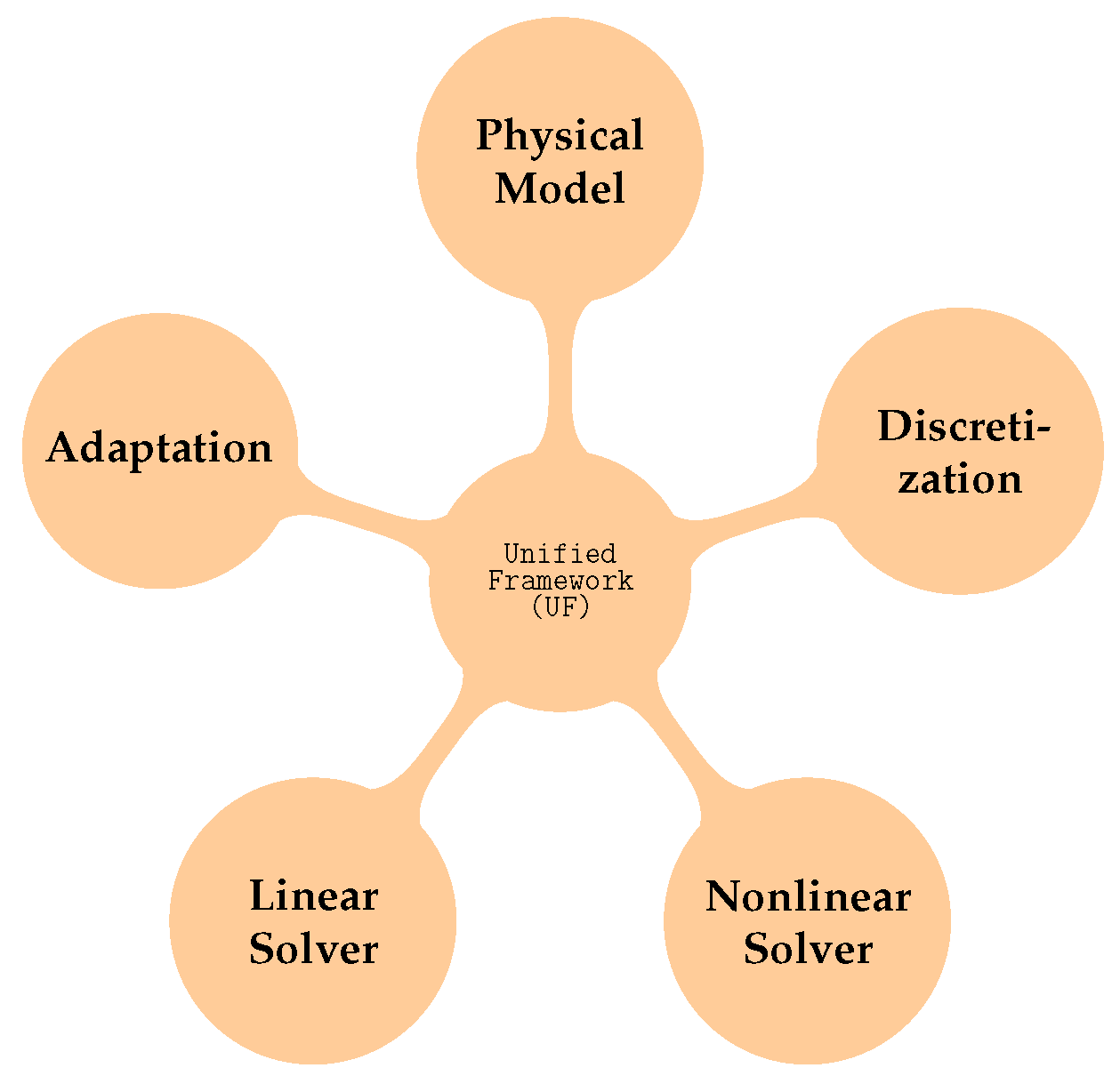
Our solver framework has a modular code structure (Figure 2). We give a brief overview only insofar as it facilitates discussing the implementation of new physical models. A more detailed documentation is given in [31].

The code is written in C++, using the Finite Element library Netgen/NGsolve [50,51]. Each module shown in Figure 2 is made available as a class, or as an external library. An example of the latter is the linear solver, which is made available through the PETSc library [52]. The most important example of the former is the physical modeling. Each model is required to implement certain functions modeling Equation (1) (convective flux, diffusive flux, boundary conditions, etc.). Listing 1 shows the class definition. The template parameters D and $COMP$ refer to the physical dimension and number of state vector components, respectively.

Listing 1. Definition of a Model.

template <int D, int COMP>

class MyModel {

…

};

Listing 1. Definition of a Model.

template <int D, int COMP>

class MyModel {

…

};

For the present work, this data structure has been enlarged to allow more flexible physical modeling, by decoupling the definition of the fluxes in the model and the closure equations used to evaluate them. We follow the Strategy pattern as defined by Gamma et al. [53] to set up a uniform interface between the general models describing the conservation laws, and families of different algorithms that implement the closure equations. A specific implementation is then linked to a model through a template parameter $CLOS$, as shown in Listing 2.

Listing 2. Model definition including new interface.

template <int D, int COMP, class CLOS>

class MyModel {

…

};.

Listing 2. Model definition including new interface.

template <int D, int COMP, class CLOS>

class MyModel {

…

};.

Physical models, such as the compressible Euler equations, can thus use different thermodynamic and transport models through well-defined interfaces. For example, the perfect gas model, as well as the model for thermally perfect gases at higher temperatures discussed in Section 2, use the same model class, but have different closure classes as template parameters. The latter includes an interface to the library Mutation++.

As an example, consider the convective flux. Convective flux evaluation is a required public function within the model class. For the Euler or Navier–Stokes equations, the implementation using the new thermodynamic interface given in Listing 3.

Listing 3. Function to evaluate the convective flux for the compressible Euler or Navier–Stokes equations.

template <typename SCAL>

static void EvalConvFlux(Vec<COMP, SCAL> & state,

SpatialParams<D> & sparam,

Mat<COMP, D, SCAL> & res) {

SCAL p;

Vec<D, SCAL> U;

CLOS::EvalPrim(state, U, p);

res = state * Trans(U);

res.Rows(1, D+1) += p * Id<D>();

res.Row(D+1) += p * U;

}

Listing 3. Function to evaluate the convective flux for the compressible Euler or Navier–Stokes equations.

template <typename SCAL>

static void EvalConvFlux(Vec<COMP, SCAL> & state,

SpatialParams<D> & sparam,

Mat<COMP, D, SCAL> & res) {

SCAL p;

Vec<D, SCAL> U;

CLOS::EvalPrim(state, U, p);

res = state * Trans(U);

res.Rows(1, D+1) += p * Id<D>();

res.Row(D+1) += p * U;

}

Please note that the thermodynamics is contained in the evaluation of the primitive variables, which is thus relegated to the new module. The structure sparam contains several mesh variables, such as the node location of the current flux evaluation. This allows implementation of fluxes that depend on the physical coordinates, although it is not needed for the Euler equations. Please note that the template parameter SCAL allows function evaluation using standard data types, as well as custom made algorithmic differentiation data types. We come back to this in Section 5.1.

All model-dependent functions are made available through such public functions. From the solver, which is itself a class, these functions can be queried. Listing 4 illustrates this for evaluation of convective and diffusive fluxes. These calls are used in the volume quadrature when assembling the residual or the Jacobian of the discretization (17).

Listing 4. Calling Model Functions from the Solver Kernel.

if    (Model::Convection)

Model::EvalConvFlux(w, sparam, fc);

if    (Model::Diffusion)

Model::EvalDiffFlux(w, q, sparam, fv);

f = fc -fv;

Listing 4. Calling Model Functions from the Solver Kernel.

if    (Model::Convection)

Model::EvalConvFlux(w, sparam, fc);

if    (Model::Diffusion)

Model::EvalDiffFlux(w, q, sparam, fv);

f = fc -fv;

The model itself is a template parameter to the main solver class (Listing 5). The code can thus be compiled to solve different physical models using the same solver kernel. Implementing new models usually requires implementation of a new (or modified) model class.

Notice that the solver also takes the same template parameters D and $COMP$ as the model. The discretization is written for arbitrary values of these parameters. For instance, the compressible Navier–Stokes equations are implemented only once. Two- or three-dimensional flow can be selected by compiling with $D=2$, or $D=3$, respectively. Moreover, models with arbitrary number of components are easily implemented.

Listing 5. The solver class.

template <int D, int COMP, class Model>

class UnifyingFramework: public NumProc {

…

};

Listing 5. The solver class.

template <int D, int COMP, class Model>

class UnifyingFramework: public NumProc {

…

};

Recall that our code is built on the library Netgen/NGSolve. In Listing 5, the inherited class NumProc is indeed a class defined in NGSolve, and may be used to register our solver as an object inside the NGSolve framework. The code is then compiled as a dynamic library which may be loaded by the NGSolve executable at runtime.

Algorithmic Differentiation

The solver is intended to function in a research environment, where modeling of different physical phenomena is frequent. The overall code structure is designed to facilitate code maintenance, as well as the implementation of new models and numerical methods. The modular structure described in the previous section follows this rationale. However, as we argued in the introduction, flexibility must extend to differentiation of physical models. An accurate differentiation of the residual function not only enables fast convergence of a Newton solver (Section 3.1), but also allows direct use of the system Jacobian in a discrete adjoint context. We therefore opted for an approach using algorithmic differentiation.

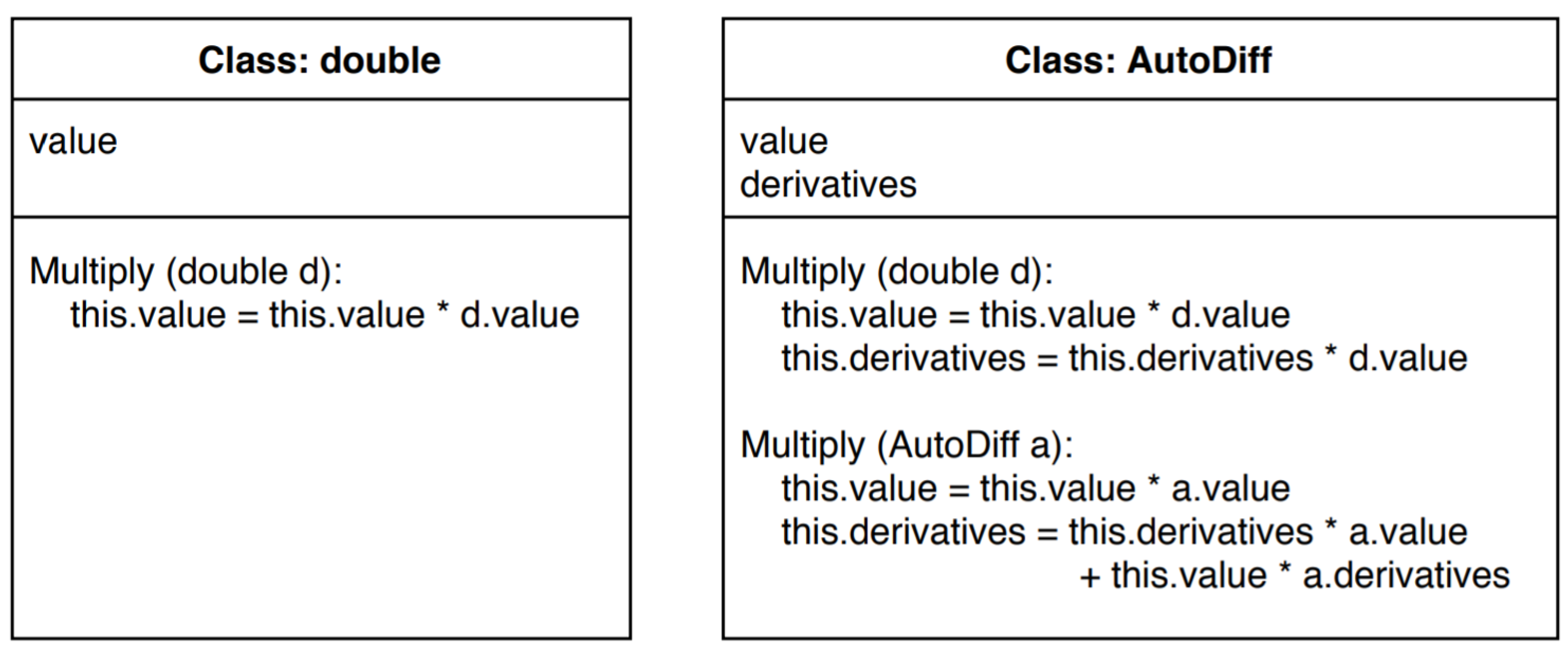
Algorithmic differentiation is implemented via a class-based data structure. The AutoDiff class, made available by the NGSolve library, carries both values and derivatives. Within the class definition, methods are defined to overload standard operations and functions. Figure 3 illustrates the concept, using multiplication as an example.

Individual routines contributing to the computation of the residual, such as the flux functions shown in Listing 3, are templated and can thus take AutoDiff arguments.

However, interfaces to undifferentiated external libraries are problematic. The most straightforward solution, if manual differentiation is not deemed economically feasible, is to use (local) finite-difference approximation. On the other hand, alternatives may be available. In particular, for some quantities computed by the library Mutation++, thermodynamic calculus may be used to fill the data structure locally with exact derivatives. As an example, consider the computation of temperature. Using the templated flux interface in Listing 3, the elements of the state vector are passed as AutoDiff types. The temperature is obtained (as a double) directly from Mutation++ as a function of the local state. The starting point for computing the derivatives is the relation for the internal energy,

$$\rho e=\sum _i^{N_s}{\rho }_i{e}_i\left(T\right)=E-\frac{\rho \mathit{v}·\mathit{v}}{2},$$

(40)

and noting $d{e}_i=c_{v,i}dT$. A straightforward computation yields

$$\frac{\partial T}{\partial {\rho }_j}=\frac{(\mathit{v}·\mathit{v})/2-e_j\left(T\right)}{{\sum }_i^{N_s}{\rho }_i{c}_{v,i}},\frac{\partial T}{\partial \rho \mathit{v}}=\frac{-\mathit{v}}{{\sum }_i^{N_s}{\rho }_i{c}_{v,i}},\frac{\partial T}{\partial E}=\frac{1}{{\sum }_i^{N_s}{\rho }_i{c}_{v,i}}.$$

(41)

One may thus instantiate the temperature as an AutoDiff by directly storing ${\nabla }_{\mathit{u}}T$ computed in this way. For frozen flow, the computation simplifies somewhat, as derivatives with respect to the individual species densities are not needed. Instead, temperature derivatives (with respect to the state) can be assigned easily using

$$e=\frac{E}{\rho }-\frac{1}{2}\mathit{v}·\mathit{v},$$

(42)

which gives the mixture internal energy as an AutoDiff (i.e., carries the derivatives), and using the mixture specific heat via $de=c_{v}dT$. The mixture specific heat can be obtained directly from Mutation++.

In either case, other variables using the temperature analytically are now automatically differentiated. In other words, they can be directly computed as an AutoDiff type without further manual input. Examples are the pressure using (4), or the viscosity using Sutherlands law (if applicable). In fact, if additionally the thermal conductivity is computed using a constant Prandtl number approximation, the frozen flow model has exact flux derivatives. If instead the transport coefficients are obtained directly from Mutation++, local difference approximations are currently used to produce derivatives for the AutoDiff type. Mutation++ can compute the derivatives of the species production rates with respect to species densities. This is used in the present work. At present, the derivatives of the species production rates with respect to the temperature are computed using finite difference approximations.

6. Results

We present numerical results using the modeling approach, discretization, and adaptation discussed in preceding Sections. Focus is on verification of the implementation, the interplay between the physical modeling, shock capturing, and the convergence of the Newton solver. The interface to the PETSc library makes is possible to use a variety of linear solvers. However, a study of linear solvers or preconditioning is not our aim. We therefore computed all results shown here with the same rather general setup, using a GMRES(m) method to solve the linear systems (where $m=120$), along with an ILU(k) preconditioner and levels of fill $3\le k\le 15$. Using the same setting for all cases allows a direct comparison between different modeling approaches, and to assess influence of the modeling and adaptive procedure on solver performance.

6.1. Verification of Thermodynamics Implementation

Initial verification of the new thermodynamics interface may be provided by considering moderate flow conditions, where the previously implemented perfect gas model ought to be valid. The new models should then yield very similar results. Subsequently, we consider a case at higher temperature, where the caloriaclly perface gas assumption ceases to be valid, and finite rate chemistry becomes important.

We shall frequently compare Models 1–3 in Table 1. In the case of the frozen flow high-enthalpy model (Model 2 in Table 1), we generally use Mutation++ to compute the transport coefficients. For all results shown below the NASA 9-coefficient polynomial database has been used with Mutation++ (see [23] and references therein for database options).

6.1.1. Laminar Flow around a Cylinder

We choose the Reynolds number small enough so that a steady flow develops. Free stream conditions are given by atmospheric pressure ($p_{\infty }=1$ atm) and moderate temperature ($T_{\infty }=298.15$) K. For the cylinder, adiabatic no-slip wall boundary conditions are used. In this setup, all models should yield very similar results. We used a low free stream Mach number $M_{\infty }=0.1$ to stay near the incompressible regime. As a secondary effect, using low Mach numbers puts additional strain on the solver, as it increases stiffness. (At present, no preconditioning for low Mach numbers is used.) Figure 4 shows the results in terms of the drag coefficient.

Adapted grids, using the method of Section 4, were created for each of these Reynolds numbers using the perfect gas model. All results for a given Reynolds number were then computed on the same grid. Solver results are compared to an empirical correlation for incompressible flow [54]. It can be seen that the new thermodynamics modules reproduce the results of the previously implemented model.

The non-equilibrium multispecies model can be used with a variety of mixture models. In Figure 4, we show results using a five-species air model. For the given flow conditions, only two species ($O_2$ and $N_2$) are significant. When computing the same case with a corresponding 2-species model, the solver yields identical results, up to the decimal accuracy used for output (

Table 2. Cylinder Test case. Results for the drag coefficient using 2-Species and 5-Species air models.

Re	2-Species Air	5-Species Air
30	1.75088641	1.75088641
45	1.48528380	1.48528380
60	1.32895637	1.32895637

). The solver is able to keep the non-significant species at machine-zero without problems during the flow evolution process. (We initialize the flow field with free-stream conditions.)

Furthermore, of interest is the convergence of the Newton solver. Figure 5 shows the convergence curves for three representative cases and different models.

Generally, we measure the residual of the globally coupled degrees of freedom by taking the $l^2$ norm of the right-hand-side of Equation (23). It can be seen that the convergence is indeed very similar for all models. The low Reynolds numbers of this test case emphasize the viscous terms. These contain the transport coefficients which are potentially approximated by finite-differences. (The differentiation of Sutherland’s law is analytic.)

6.1.2. Post-Shock Relaxation

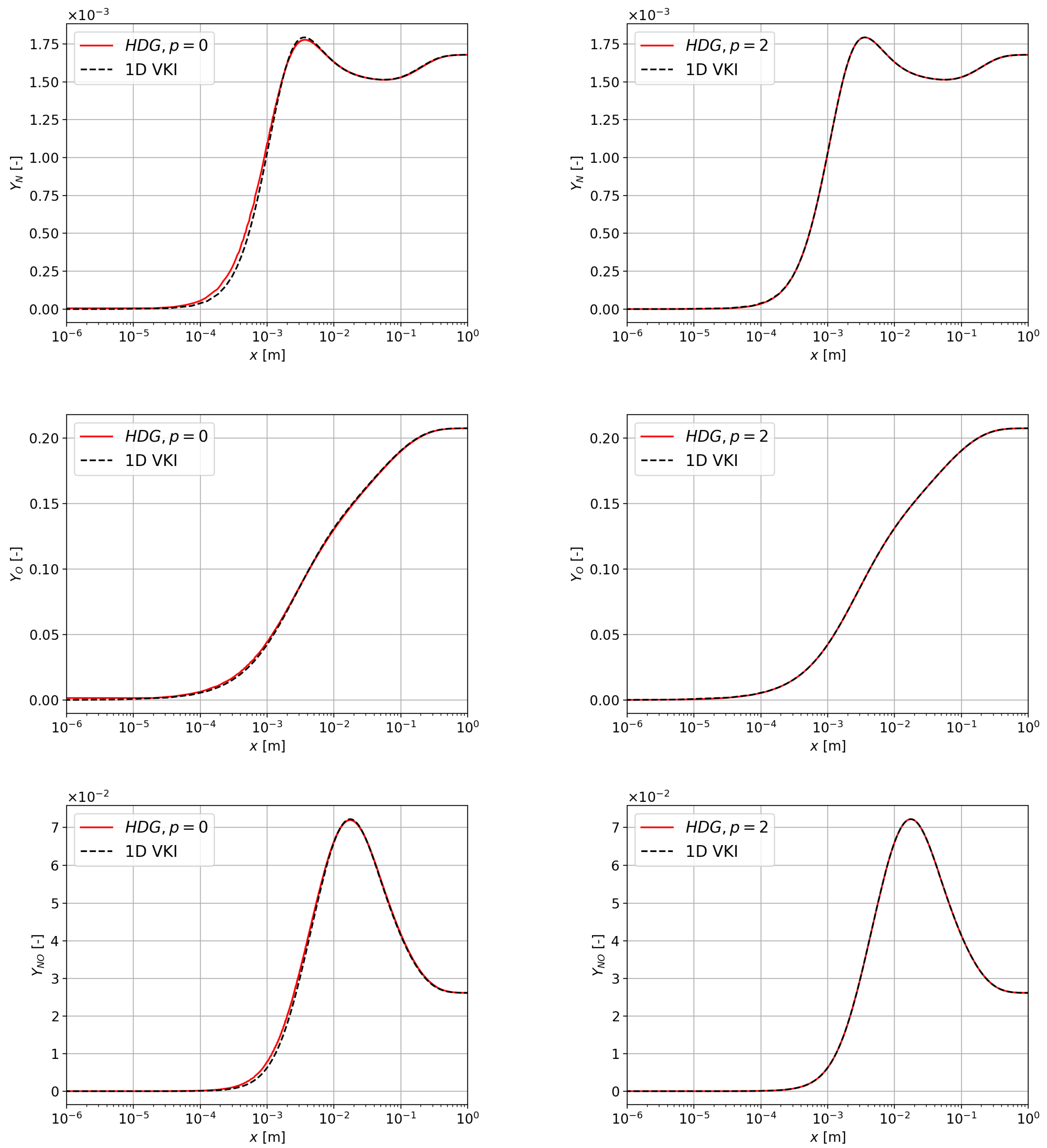
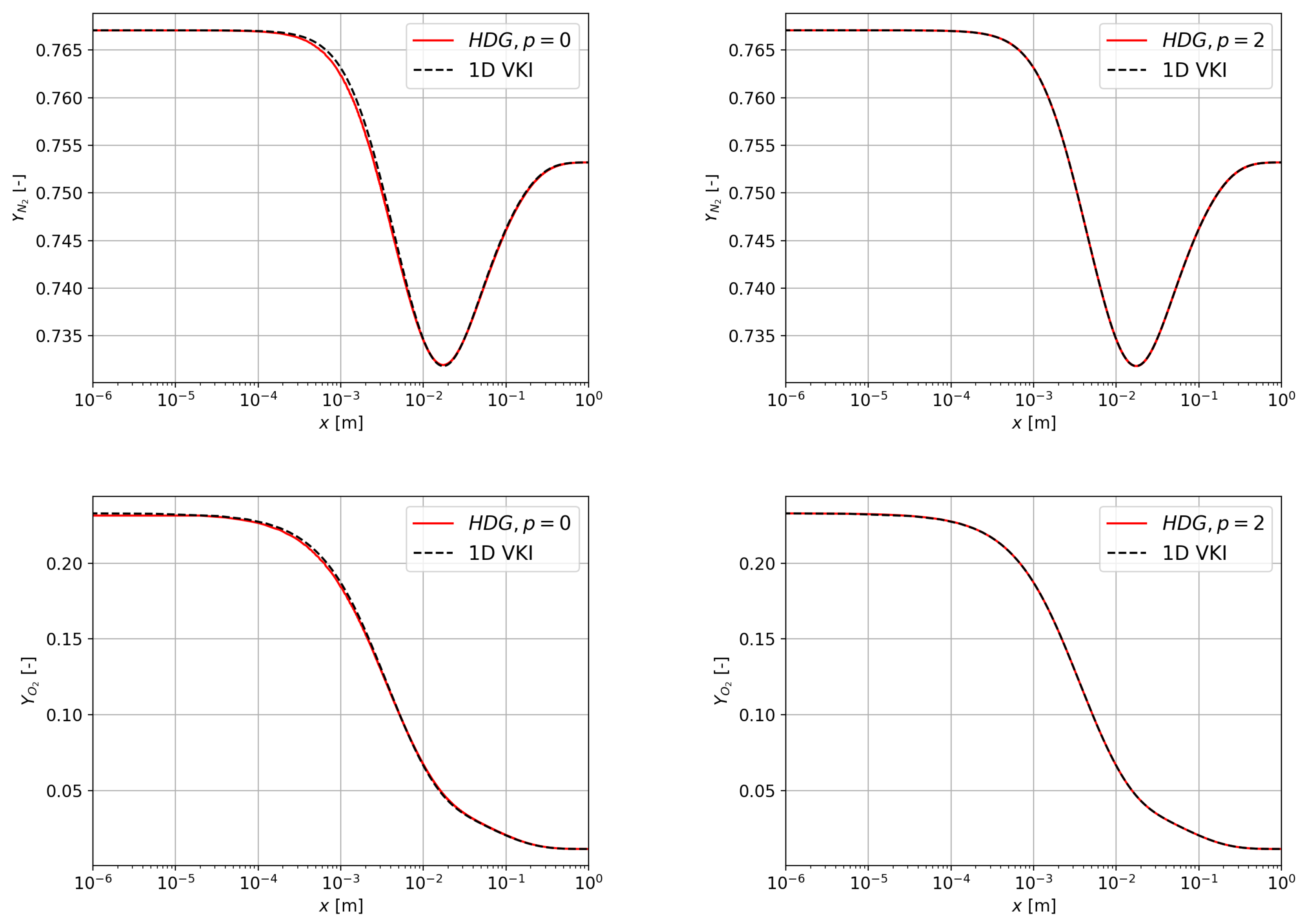
We consider a simulation of flow relaxation to chemical equilibrium behind a strong normal shock.

Table 3. Pre- and post-shock conditions for the shock relaxation test case.

	T [K]	p [Pa]	u [m/s]
Pre-shock	300	100	4000
Post-shock	6539	16,101	542

shows the pre- and post-shock conditions of the flow.

Across the shock, the chemistry is assumed to be frozen. Thus, the immediate post-shock species composition is identical to the pre-shock composition. This composition, together with the post-shock flow conditions, are assumed as inflow conditions for our computation. Not that this inflow state is far from equilibrium. The flow relaxes toward chemical equilibrium, as it proceeds downstream the shock. Similar cases have previously been used by several researchers [36,55,56,57]. We use a five-component, single-temperature inviscid air model with Mutation++ (Model 3 in Table 1). We compare our results to an independently verified 1D code, produced at the von Karman Institut for Fluid Dynamics, which also uses Mutation++ [58].

To simulate this one-dimensional case, a thin slab of $1.5\mathrm{m}\times 0.002\mathrm{m}$ with a graded mesh of approximately 1500 triangles was created, concentrating elements at the domain inlet. At the left and right boundaries, inlet and outlet conditions are used, respectively, imposing the mass fractions, temperature and velocity, respectively, the pressure. Slip-wall boundary conditions in transverse direction were used.

Figure 6 and Figure 7 show the results of the simulation.

There is excellent agreement between the output of the reacting Euler model implemented in the HDG framework, and that of the 1D VKI code.

6.2. High–Mach–Number Flow

We are particularly interested in the interplay between the metric-based adaptation, shock capturing, and modeling. We shall consider flows in the supersonic to moderately hypersonic regime. Shock capturing terms are available for the frozen flow models, i.e., Models 1 and 2 in Table 1, which will be used in this section. (As we stated in Section 3.1, our shock-capturing method is able to reliably resolve shocks up to around $M_{\infty }\approx 8$.) We consider external aerodynamics, and to avoid additional complications from the ensuing high Reynolds numbers, inviscid flow.

6.2.1. Diamond Profile

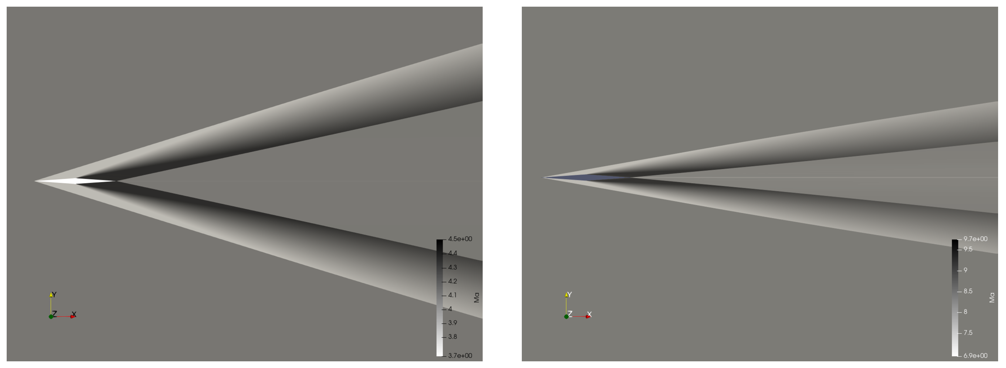
In this section, we solve inviscid supersonic to hypersonic flow around a diamond-shaped profile. The geometry of the profile is defined by a wedge angle of ${10}^{\circ }$, and a chord length of $c=1$. Free-stream Mach numbers ranging from $M_{\infty }=2$ to $M_{\infty }=8$ were used, along with adiabatic slip-wall boundary conditions at the airfoil. Figure 8 shows two representative Mach number contour plots.

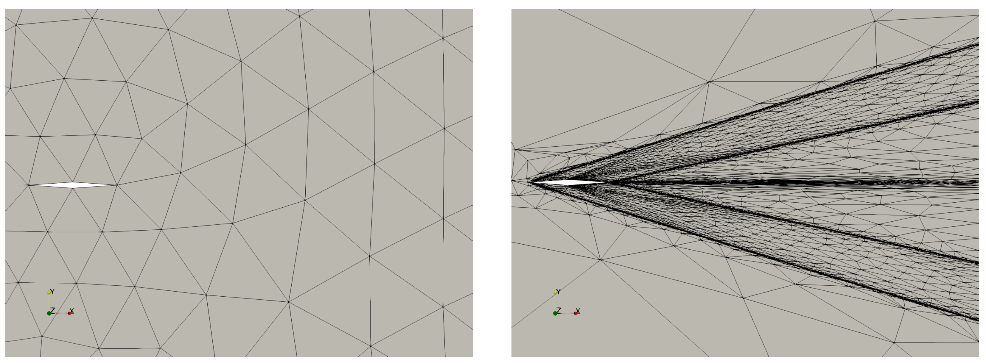
Results are computed on adapted meshes. Figure 9 shows the initial mesh used for all cases in this section, as well as a representative mesh produced by the adaptation sequence. The complexity constraint in Equation (37) is increased by $20\%$ in each adaptation cycle. This produces successively finer meshes, each of which with optimized distribution of degrees-of-freedom (cf. Section 4).

For the perfect gas model, the exact solution for the drag coefficient can be computed from the shock-jump relations and Prandtl-Meyer expansion around the tip of the airfoil. The left plot in Figure 10 shows a comparison between the exact values and the solution computed on adapted grids.

The high-temperature models admit calorically imperfect gases. For this model the perfect-gas solution for the drag is not exact. Nevertheless, deviations are relatively small, and the perfect gas solution has been used as a reference value for all models. Figure 10 shows the convergence of the drag coefficient as a function of the number of mesh elements. Both the perfect gas model and the high-temperature model produce a solution within $1\%$ of the drag value on relatively coarse meshes. Empirically, it has been found that the convergence as a function of DoF is fairly insensitive to the amount by which they are increased. The regeneration of the mesh, based on the metric, results not only in increase of DoF, but also in redistribution. As a consequence, a higher fraction of the added DoF (and even the existing DoF) can be placed in critical regions, and thus be leveraged more effectively.

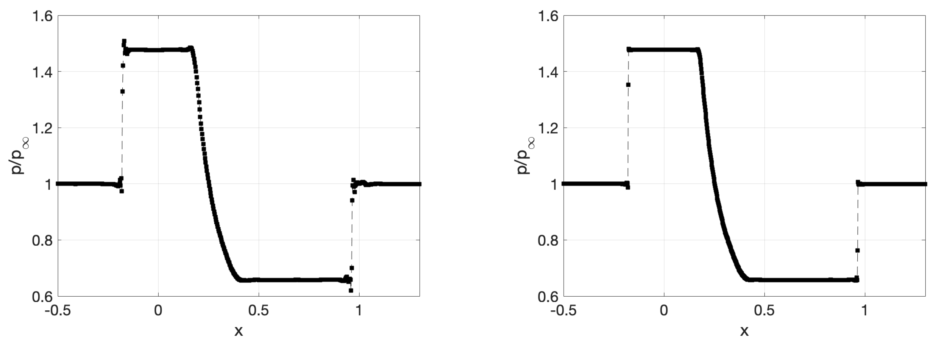
As we discussed in Section 3.1, we use a generic shock-capturing term. Up to the Mach numbers discussed here, shocks are captured cleanly. Moreover, the adaptation process, which is able to isolate shocks on anisotropic elements, is an important ingredient in the overall shock-capturing approach. In fact, up to moderate Mach numbers, the adaptation and the diffusion injected by the numerical fluxes sufficiently stabilize the solution, and converged solutions can be obtained without nonlinear stabilization provided by the shock capturing term. A representative result is shown in Figure 11.

For higher Mach number, the oscillations produced at discontinuities become significant enough to impede the convergence process, and the shock capturing term must be used to obtain fully converged steady-state solutions.

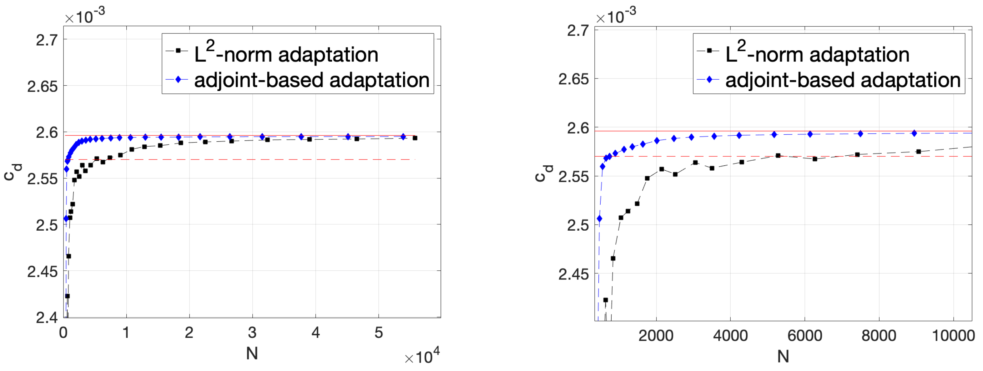
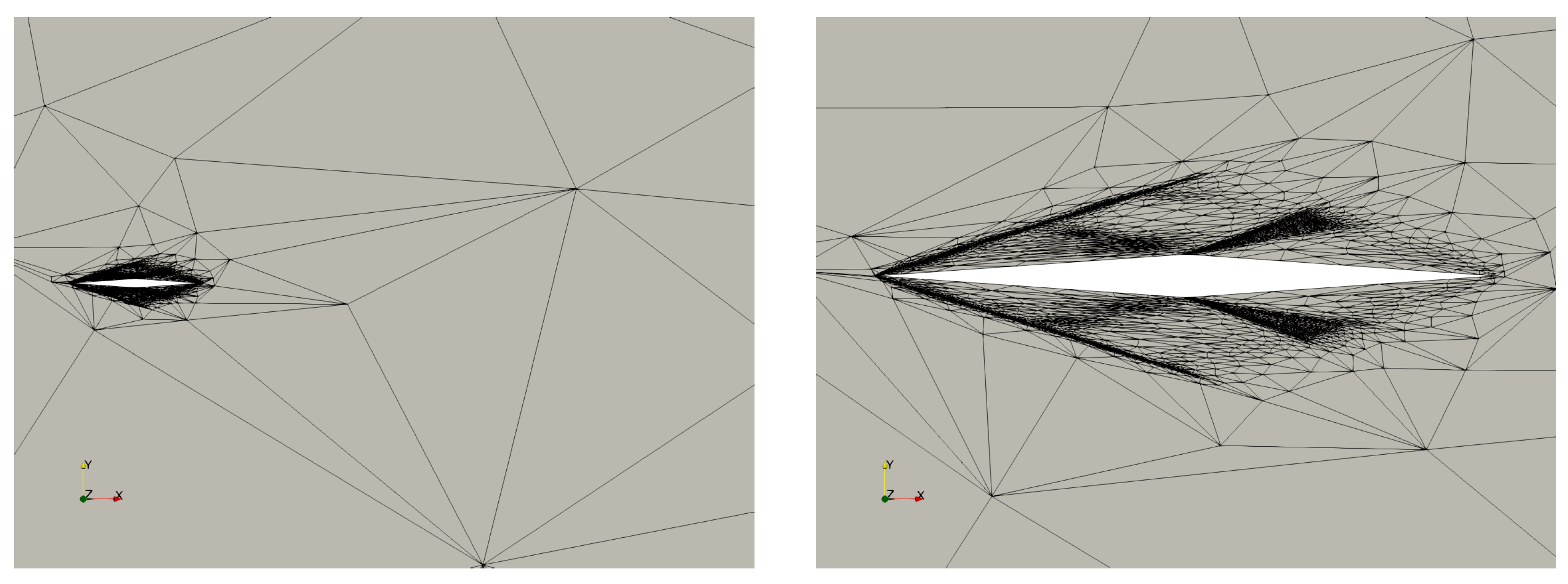
Convergence of force coefficients can be dramatically improved with goal-oriented adaptation. For this purpose, we used the methods of Section 4 with the adjoint-based modification discussed in [22]. Figure 12 shows a representative mesh produced when adapting on the drag coefficient.

Clearly, the shock is not resolved beyond the near field. In contrast, as we showed in Figure 9, norm-based optimization will resolve the entire shock into the farfield, irrespective of whether or not this is necessary for accurate computation of the drag. The goal-oriented approach can thus potentially save a large number of degrees of freedom. Indeed, Figure 13 demonstrates that adjoint-based adaptation leads to much better convergence in the target quantity.

Finally, Figure 14 shows the convergence of the nonlinear solver on adapted grids.

These curves are representative for the convergence on all the adapted meshes. Exceptions to the pattern of reliable convergence begin to emerge for $M_{\infty }=8$, where a few runs on intermediate adapted meshes did not fully converge. (For $M_{\infty }=4$ all runs converged to machine zero.) The rightmost plot in Figure 14 shows an example, where the residual convergence stalls after a reduction of about three orders of magnitude. For even higher Mach numbers, as we mentioned in Section 3.1, the currently implemented generic shock-capturing procedure is not expected to be the best choice.

6.2.2. NACA 0012

Consider supersonic to hypersonic inviscid flow around the NACA0012 airfoil. This case is somewhat more challenging, as it includes a stronger normal shock along the stagnation line, and a curved shock, bending into the farfield. Again, we use goal-oriented adaptation, based on the drag coefficient. Figure 15 and Figure 16 show adapted meshes.

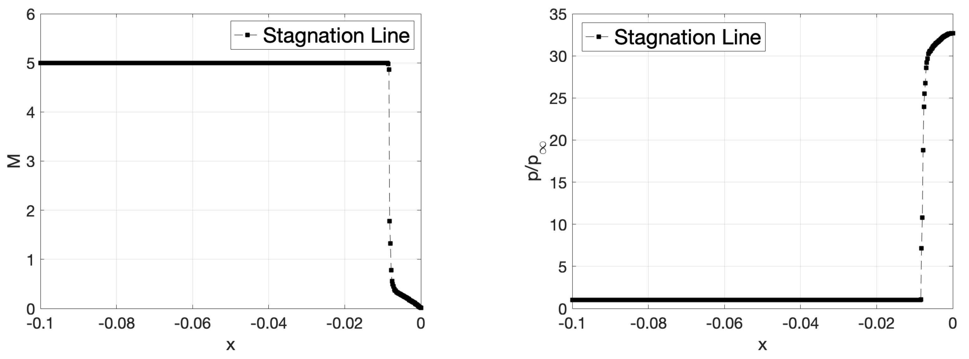
Shock are again resolved only as far as necessary for the computation of the drag coefficient. For free stream conditions $M_{\infty }=5$, Figure 17 shows a plot of Mach number and pressure along the stagnation line, using the solution obtained from the high-enthalpy frozen flow model (Model 2 in Table 1). It is clearly visible that the shock is well-captured.

7. Conclusions and Outlook

We presented design and initial verification of a high-order, HDG-based solver for high-speed flows, and, more broadly, flows requiring non-trivial physical modeling. We used object-oriented programming, and algorithmic differentiation (AD), to encapsulate different aspects of the modeling. Fluxes, source terms, and boundary conditions are implemented inside a model class, which is made available to the solver as a template parameter. These functions are differentiated automatically using the AD data structure. Closure equations and transport coefficients are implemented in a separate class, made available to the model, again as a template parameter. This hierarchical approach allows fairly flexible, non-intrusive implementation of physical models, and will thus serve as a stepping stone for future endeavors. For example, work is underway to implement modeling for flows in local thermodynamic equilibrium (LTE), as well as plasma flows. In addition, the shock capturing mechanism needs to be extended to multispecies non-equilibrium models and higher Mach numbers.

Moreover, future work will focus on more extensive validation campaigns regarding species diffusion and, in particular, heat flux into surfaces. In this context, extensions are planned to deal with gas-surface interaction on catalytic surfaces. This requires more complex boundary conditions than those considered in the present paper. Nevertheless, the same data structure can be used.

Efficient simulation of compressible flows using high-order methods requires adaptation. The metric-based approach was shown to be a very promising approach for high-speed flow. Moreover, the AD data structure in conjunction with adjoint-consistent discretization enables one to use a discrete adjoint approach for new physical models without implementation overhead. The adjoint-based approach leads to superior results, provided a suitable target of the computation can be identified. In the present paper, drag has been used. However, heat flux, in conjunction with non-adiabatic walls, is also a viable target, and will be considered in future work.