Classification and Analysis of Go-Arounds in Commercial Aviation Using ADS-B Data

Abstract

Go-arounds are a necessary aspect of commercial aviation and are conducted after a landing attempt has been aborted. It is necessary to conduct go-arounds in the safest possible manner, as go-arounds are the most safety-critical of operations. Recently, the increased availability of data, such as ADS-B, has provided the opportunity to leverage machine learning and data analytics techniques to assess aviation safety events. This paper presents a framework to detect go-around flights, identify relevant features, and utilize unsupervised clustering algorithms to categorize go-around flights, with the objective of gaining insight into aspects of typical, nominal go-arounds and factors that contribute to potentially abnormal or anomalous go-arounds. Approaches into San Francisco International Airport in 2019 were examined. A total of 890 flights that conducted a single go-around were identified by assessing an aircraft’s vertical rate, altitude, and cumulative ground track distance states during approach. For each flight, 61 features relevant to go-around incidents were identified. The HDBSCAN clustering algorithm was leveraged to identify nominal go-arounds, anomalous go-arounds, and a third cluster of flights that conducted a go-around significantly later than other go-around trajectories. Results indicate that the go-arounds detected as being anomalous tended to have higher energy states and deviations from standard procedures when compared to the nominal go-arounds during the first approach, prior to the go-around. Further, an extensive comparison of energy states between nominal flights, anomalous flights, the first approach prior to the go-around, and the second approach following the go-around is presented.

1. Introduction and Background

A go-around is a maneuver performed by a pilot after a decision has been made to discontinue a landing attempt. Go-arounds are conducted for a variety of reasons, including unstable approach, adverse weather, degraded conditions on the runway, a request by air traffic control (ATC), etc. An unstable approach is said to occur when an aircraft does not maintain either its speed, descent rate, glide slope, or localizer on approach [1]. While a single short-haul commercial airline pilot may only conduct a go-around at a rate of once or twice per year, cumulatively, go-arounds occur at an average rate of one to three per 1000 commercial flight approaches [2]. Due to the frequency of go-arounds, they may be considered a relatively significant event in commercial aviation operations. Further, it is noted that one in ten go-arounds record a potentially hazardous outcome [2]. Therefore, go-arounds are an important event to investigate to contribute to improving overall aviation safety.

Much of the current aviation literature focuses on detecting the occurrence of go-arounds, detecting conditions that should warrant the execution of a go-around, and, sometimes, qualitatively evaluating the underlying causes of go-arounds. The Flight Safety Foundation [2] surveyed pilots and crew members and examined 64 go-around reports between 2000 and 2012 to examine factors that went into go-around decision-making as well as the outcome of the go-around. The study, which focused on examining and proposing guidelines to improve go-around non-compliance, used the data collected to analyze and make several recommendations concerning stable approach criteria and go-around guidelines. Go-around non-compliance is when pilots do not follow established company (airline) policies for when a go-around should be conducted [2]. Campbell et al. [3] similarly sought to develop criteria for go-around decision-making. However, this study differed in that a flight simulator was utilized to evaluate crew touchdown performance under varying conditions at go-around decision points, or gates [3]. Campbell et al. concluded that the go-around decision point should be between the 100 ft and 300 ft gates, where reference speed and localizer deviations had the most significant influence on the go-around decision [3]. Additionally, Karboviak et al. [4] developed a “Go-Around Detection Tool” for General Aviation (GA) to classify whether approaches are a go-around, touch-and-go landing, or stop-and-go landing. Additionally, the tool could detect whether approaches were stable or unstable. The tool utilized flight data recorder parameters and achieved a 98.14% accuracy. Karboviak et al. [4] found that only 20.62% of unstable approaches resulted in a go-around.

Recently, the increased availability of flight trajectory data has enabled the utilization of machine learning and data analytics techniques to assess aviation safety events [5]. Specifically, the introduction of Automatic Dependent Surveillance–Broadcast (ADS-B) technology has created abundant opportunities to analyze flight trajectory data. ADS-B is a surveillance technology that enables an aircraft to broadcast its trajectory information, determined using satellite, inertial, and radio navigation [6]. With the mandated expansion of ADS-B, open-sourced flight trajectory data became more readily accessible [7]. As of 1 January 2020, aircraft flying in controlled United States airspace are required to be equipped with ADS-B technology [8]. The overarching objective of this work is to leverage trajectory information available in the open-source ADS-B data to develop a method to characterize go-arounds in commercial aviation.

Stemming from the increased availability and accessibility of aviation trajectory data, machine learning techniques have been gaining traction among aviation safety researchers interested in detecting and/or predicting go-arounds using historical flight data. Bro [9] trained an artificial neural network to categorize a landing event as a go-around using historical GA flight data, where low error rates were achieved. Wang et al. [10] examined the feasibility of training a logistic regression model on surveillance track data for 8158 approaches to Newark International Airport (KEWR) to predict the likelihood of a stable approach. The accuracy rates were 61.7%, 73.6%, and 83.1% for gates at 10 nm, 6 nm, and 3 nm, respectively. Proud [8] analyzed one year of ADS-B approach data at Chhatrapati Shivaji Maharaj International Airport Mumbai (VABB) to compare four existing methods to detect go-arounds. Proud also developed a novel method leveraging fuzzy logic to characterize different flight phases and examined changes in flight phases to detect a go-around [8]. Proud demonstrated that his method has a significantly higher accuracy rate than existing detection algorithms and applied his method to demonstrate that the majority of go-arounds at VABB can be attributed to weather and unstable approaches.

Additionally, existing research focuses on leveraging historical data to examine the causes of these go-arounds. Subramanian and Rao [11] used the NASA ASRS database to analyze go-around and missed approach data for GA. Subramanian and Rao first classified each incident based on 20 identified factors [11]. Subramanian and Rao then trained a Long Short-Term Memory (LSTM) neural network to forecast the count for each incident type [11]. The LSTM neural network enabled the identification of factors that contributed to incident trends [11]. Sherry et al. also utilized the NASA ASRS database to identify potential causes of aborted approaches, which they defined as “go around for a Missed Approach as well as a turn off the final approach segment prior to the Missed Approach Point (MAP)” [12]. They found airplane issues (unstable approach, alerts, and on-board failures) to be the largest factor leading to an aborted approach. The current work does not differentiate between aborted approaches as defined by them and traditional go-arounds and includes both. Janakiraman et al. [13] developed an algorithm for the automatic discovery of precursors in time-series data (ADOPT). The ADOPT algorithm was applied to go-around flights to identify several precursors, including energy mismanagement and potential overtake [13]. Dai et al. [14] focused on determining the impact of specific factors of interest on go-around occurrence. First, go-arounds at John F. Kennedy International Airport (KJFK) were detected utilizing a trajectory-based approach [15]. Subsequently, the impact of various features, such as separation, airport conditions, weather conditions, and trajectory performance, on go-around occurrence were modeled using a principal component logistic regression model [15]. Dai et al. found that there is not one dominant factor affecting go-around occurrence; however, aircraft state, visibility, ceiling height, aircraft type, and separation and speed difference from the aircraft in front are prominent factors. Some recent work has also focused on process-based and crew-centered go-around procedure design [16].

While there exists much literature focused on detecting go-arounds, conditions that should warrant a go-around decision, and causes of go-arounds, limited work has been conducted related to the characterization of go-arounds. Thus, a gap exists in the literature regarding a comprehensive method to characterize go-arounds. Further, existing methods examine the features of all approaches to determine casual factors, to detect go-arounds, or to perform adjacent analyses. The objective of this work is to leverage the full time-series of go-around flight trajectories. While go-arounds are a necessary aspect of operations, they are also among the most safety-critical ones as the pilots’ workload is relatively high during this phase. Therefore, there exists a need to study go-arounds such that actionable insights may be obtained related to their operations. It is imperative to execute go-arounds in the safest possible manner to avoid accidents or hazards. Therefore, the overarching research objective of this work is to leverage machine learning techniques and open-source ADS-B data to:

1

Classify go-arounds to gain insight into the aspects of typical, nominal go-arounds;

2

Identify factors that contribute to abnormal or anomalous go-arounds.

The remainder of this paper is organized as follows. Section 2 details the methodology by which go-arounds are detected in an ADS-B data set. Subsequently, Section 3 presents results obtained after the implementation of the methodology. Finally, Section 4 concludes the paper.

2. Methodology

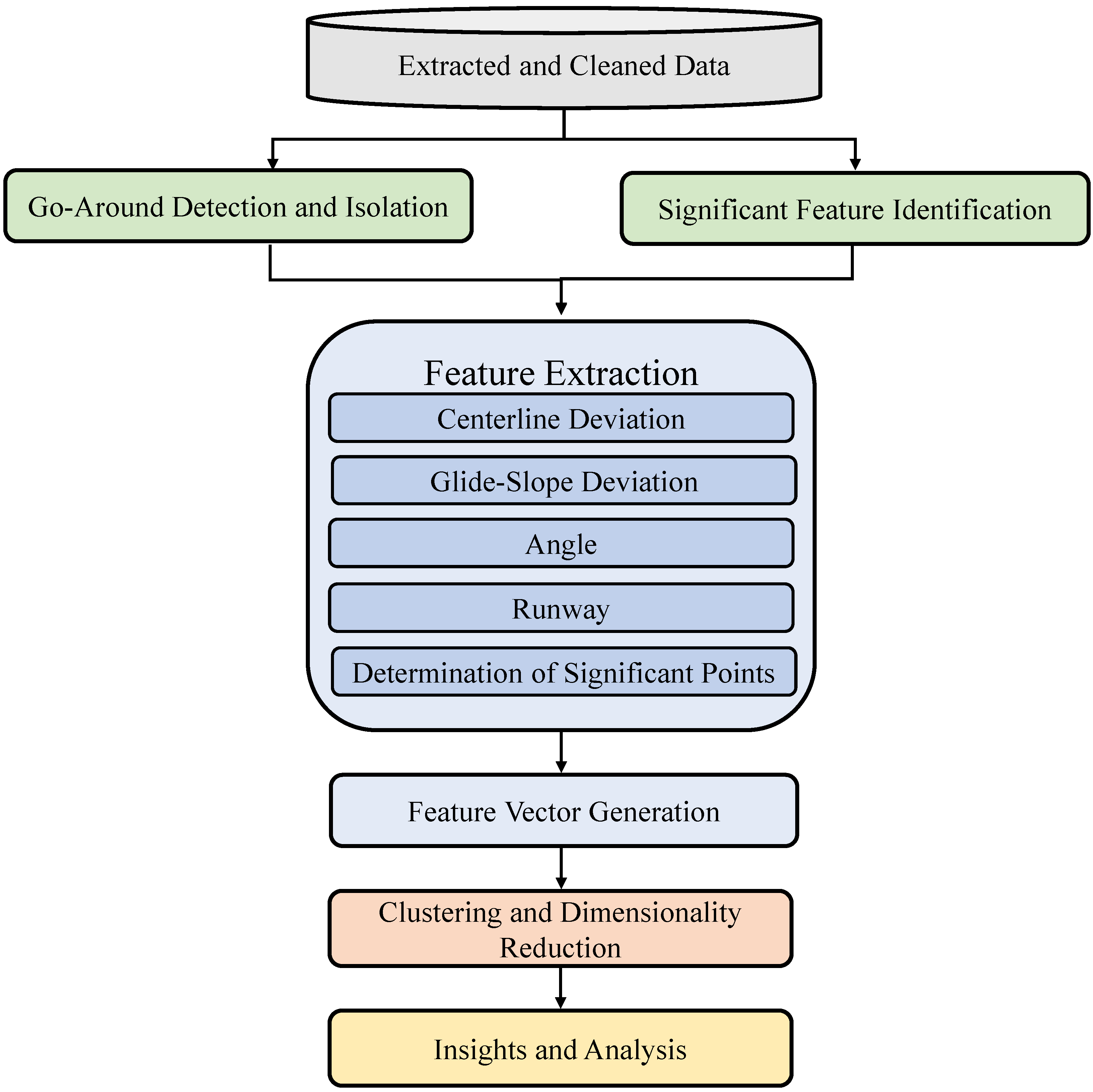
Figure 1 displays a summary of the methodology applied. First, the data extraction, cleaning, and processing is discussed. Then, a discussion of the detection of go-around flights and the identification of significant trajectory points and features is presented. Steps to extract significant features at each of the points are then discussed in detail, as well as the process of generating the feature vector. Finally, a discussion of various clustering techniques, including those implemented, and dimensionality reduction for visualization is presented.

2.1. Data

Automatic Dependent Surveillance–Broadcast (ADS-B) trajectory data for flights arriving at San Francisco International Airport (KSFO) in 2019 were extracted from the OpenSky Network [17] historical database. The OpenSky Network [17] is a non-profit association that processes and archives ADS-B data from a global network of sensors. OpenSky Network data have previously been used by researchers for a diverse range of studies. The traffic [18] Python library enables the extraction of OpenSky Network historical ADS-B trajectory data, where each data record is referred to as a state vector. State vectors contain timestamps (added on the receiver side, with many receivers equipped with a GPS nanosecond precision clock), transponder unique 24-bit identifiers (icao24), space-filled 8-character callsigns, latitude, longitude (in degrees), (barometric) altitude (in feet, with respect to standard atmosphere), GPS altitude (in feet), ground speeds (in knots), true track angle (in degrees), vertical speed (in knots).

The procedure for cleaning and processing the OpenSky Network data applied in this work is detailed in prior work by the authors [19,20]. State vectors within a 25 nautical mile radius of KSFO and below 25,000 feet in altitude for all days in 2019 were extracted using the traffic Python library. An initial cleaning step first took place in which state vectors not meeting certain criteria were discarded, i.e., those that were repeated, empty, or associated with non-commercial flights. Next, flight segments were identified by callsign and timestamps, and a touchdown point was identified. Finally, final cleaning of the data set occurred, in which segments that were not arrival segments were discarded, and a height above ground level and cumulative ground track distance were computed for each trajectory point. Each flight was re-sampled to contain 200 data points. The final data set contained 179,538 total arrival flight segments from 1 January 2019 to 31 December 2019.

2.2. Detection of Go-Arounds

A procedure to detect go-arounds in the extracted and cleaned ADS-B trajectory data was developed. The procedure builds upon routines presented by Proud [8] and Dai [15]. Algorithm 1 presents the detailed steps to detect go-arounds. The algorithm utilizes altitude, vertical rate, and the cumulative ground track distance to detect each go-around. Existing methods to detect a go-around check for increasing altitude or a positive rate of climb at different position reports following the minimum altitude [8]. In the current work, vertical rate was assessed. Additionally, altitude checks were performed similarly to Proud [8] and Dai et al. [15] to ensure that flights in a holding pattern were not classified as go-arounds. Detected go-arounds were validated based on visual inspection of altitude and track. A total of 890 go-around flights were identified by this algorithm for use in this work.

Algorithm 1: Detects whether a given flight conducted a go-around.

Input: ADS-B time-series flight data sorted in descending order by cumulative ground track distance  $idx\leftarrow 0$;  $cgtd\leftarrow$ Cumulative ground track distance at idx;

2.3. Selection of Significant Points and Features

Significant features must be selected to apply machine learning or data mining techniques. This section outlines the rationale and historical insights that aid in the selection of features for the clustering analysis. To select points, the process of a go-around can be divided into four main parts: (1) the approach for the initial landing that required a go-around, (2) the climb out during the go-around, (3) constant altitude hold when flying the go-around trajectory, and (4) the approach for the landing that was successful following the go-around. Captain Ed Pooley, after reviewing 66 historical go-around incidents, noted that risk-bearing unsafe go-arounds are likely to have been preceded by significant procedural non-compliance(s) [21]. This motivated the examination of the initial approach prior to the go-around. During the initial approach, pilots may go-around if they determine that the approach is unstable [3]. In his study, Pooley found that 40 events followed unstabilized flight and that 73% of these events were followed by a risk-bearing go-around [21]. Therefore, stable approach gates are used as significant points on the initial landing attempt. Generally, stable approach criteria are assessed at 1000 feet at instrument meteorological conditions (IMC) and 500 feet at visual meteorological conditions (VMC) [1]. However, out of the 890 go-arounds considered in this study, 436 flights conducted a go-around before reaching the 500-feet altitude gate. Additionally, the 1000-feet approach gate was where the final landing configuration was selected [2]. Therefore, only the 1000-feet approach gate was considered.

Blajev et al. [2] mentioned that the 1000-feet approach gate may be variable from 800 feet to 1500 feet based on the aircraft type. The highest altitude value in this spectrum, 1500 feet, was selected to include another approach gate. Dai et al. [14,15] selected factors of interest based on a literature review to reveal causal correlations that led to go-arounds. Dai et al. chose to include flight-specific features at a point five nautical miles away from the runway [15]. Dai et al. found that if the aircraft are aligned with the extended runway centerline at this point, go-arounds would decline by 9.5% [14]. Using a standard three-degree glide-slope, the aircraft would be at approximately 1592-feet altitude five nautical miles away from the runway, further bolstering the rationale of a 1500-feet approach gate. Approach gates for the successful landing following the go-around are selected in a similar manner. The 1000-feet and 500-feet approach gates were selected for this approach as they are commonly used approach gates to check for unstable approach [1,2]. As initiating a go-around ineffectively may lead to a loss of control [2], factors at the minimum altitude prior to the go-around, where a pilot would be in the beginning stages of initiating a go-around, were examined. Since the altitude at which a go-around is initiated may lead to risks, the minimum altitude prior to the go-around was considered in order to allow effective comparison between flights.

After reviewing the literature, pilot surveys, and a workshop, Campbell et al. [3] revealed five important features of interest at the approach gates: gate height, localizer deviation, glide-slope deviation, reference speed deviation, and rate of descent. Therefore, these features were selected and considered at each of the gate heights and the minimum altitude prior to the go-around. Due to the difficulty of consistently determining the reference speed for each flight (factors such as aircraft weight would have to be approximated), instead, the velocity at the approach gates was considered as a feature. Additionally, to estimate how far from the runway each of the flights were at the various approach gates, the distance between the aircraft and the runway was considered. Finally, as studies have shown, aircraft energy states affect the execution of a go-around [2,14,22]; thus, the specific total energy at all points was considered.

Aircraft pitch, early turns, and thrust are considered important during the execution of a go-around, where failure to properly manage these can increase the likelihood of an unsafe go-around [2,22]. The 1000-feet and 2500-feet altitude gates were selected to evaluate the climb following the minimum altitude prior to the go-around; 1000 feet was selected to evaluate the flight soon after the go-around decision and 2500 feet was selected as it is the half-way point during the climb for most flights. Most go-around flights reached an altitude hold at 5000 feet. As data for aircraft attitude were not directly available, features such as velocity and vertical rate were considered at these points. Additionally, to appropriately account for turns for all flights and their position at various points with respect to the go-around runway, the angle between the aircraft and the go-around runway was considered at every point.

In the past, pilots and flight instructors have expressed difficulties in capturing the go-around altitude [22]. Therefore, the point at which the aircraft reached its maximum altitude hold was selected. There are risks during the go-around associated with not following the correct trajectory [2], where pilots and flight instructors have expressed difficulty with horizontal flight path management [22]. Therefore, the half-way point of the maximum altitude hold and the point at which the aircraft began descent from the maximum altitude point were selected to evaluate features of the flight throughout the trajectory. Velocity was selected as a feature at these points as energy metrics are commonly identified as significant during a go-around [2,14,22]. Since pilots have also expressed difficulty with vertical flight path management [22], vertical rates at these points were also included.

Table 1. Summary of the significant points and features selected.

Significant Points	Altitude	Velocity	Vertical Rate	Distance to Runway	Specific Total Energy	Glide-Slope Deviation	Centerline Deviation	Angle to Runway
1500-Feet Approach Gate Prior to Go-Around		✓	✓	✓	✓	✓	✓	✓
1000-Feet Approach Gate Prior to Go-Around		✓	✓	✓	✓	✓	✓	✓
Minimum Altitude Prior to Go-Around	✓	✓	✓	✓	✓	✓	✓	✓
1000-Feet on Climb Following Go-Around Initiation		✓	✓		✓			✓
2500-Feet on Climb Following Go-Around Initiation		✓	✓		✓			✓
Start of Maximum Altitude Hold Following Go-Around Initiation		✓	✓		✓			✓
Half-Way Point of Maximum Altitude Hold		✓	✓		✓			✓
Aircraft Begins Descent for Second Approach		✓	✓		✓			✓
1000-Feet Approach Gate on Second Approach		✓	✓	✓	✓	✓	✓	✓
500-Feet Approach Gate on Second Approach		✓	✓	✓	✓	✓	✓	✓

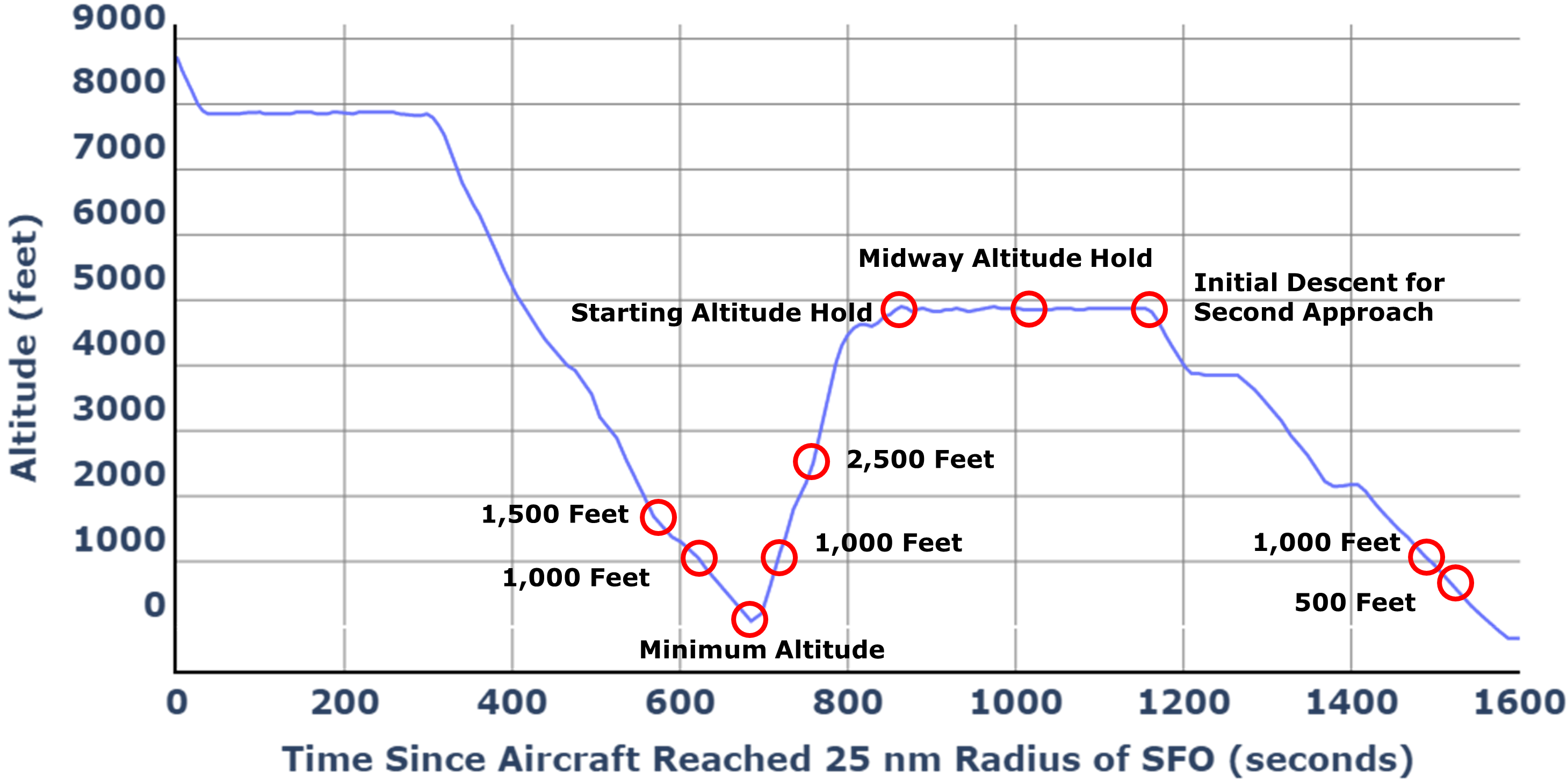
provides a summary of all of the selected points and features noted above. Figure 2 displays a visualization of the significant points throughout the go-around trajectory. The time between some of the specific points discussed above is also included. While the points discussed above are adequate to provide a snapshot of different features, incorporating a time metric allows for a better understanding of the velocities, trajectory, and energy management of the entire flight.

Table 2. Summary of the time-series features selected.

Start Time Point	End Time Point
1500-Feet Approach Gate Prior to Go-Around	Minimum Altitude Prior to Go-Around Execution
Minimum Altitude Prior to Go-Around Execution	Start of Maximum Altitude Hold Following Go-Around Initiation
Minimum Altitude Prior to Go-Around Execution	500-Feet Approach Gate on Second Approach
Start of Maximum Altitude Hold Following Go-Around Initiation	Aircraft Begins Descent for Second Approach
Aircraft Begins Descent for Second Approach	500-Feet Approach Gate on Second Approach

provides a summary of the time features selected.

2.4. Feature Engineering

The extracted and cleaned ADS-B data set contains data for many features that are leveraged, including latitude, longitude, height above ground level, velocity, vertical rate, time, specific kinetic energy, and specific total energy.

For the computation of features such as centerline deviation, glide-slope deviation, runway angle, and distance, and to determine the landing runway and go-around runway, each latitude and longitude pair was projected onto a Universal Transverse Mercator (UTM) coordinate system using a UTM-WGS84 converter for Python (https://pypi.org/project/utm/, accessed on 1 September 2021). Latitude and longitude values for each runway were obtained from the AirNav website (https://www.airnav.com/airport/SFO, accessed on 1 September 2021). The following subsections outline some of the computations performed on the data to obtain the engineered features used in this work.

2.4.1. Centerline Deviation

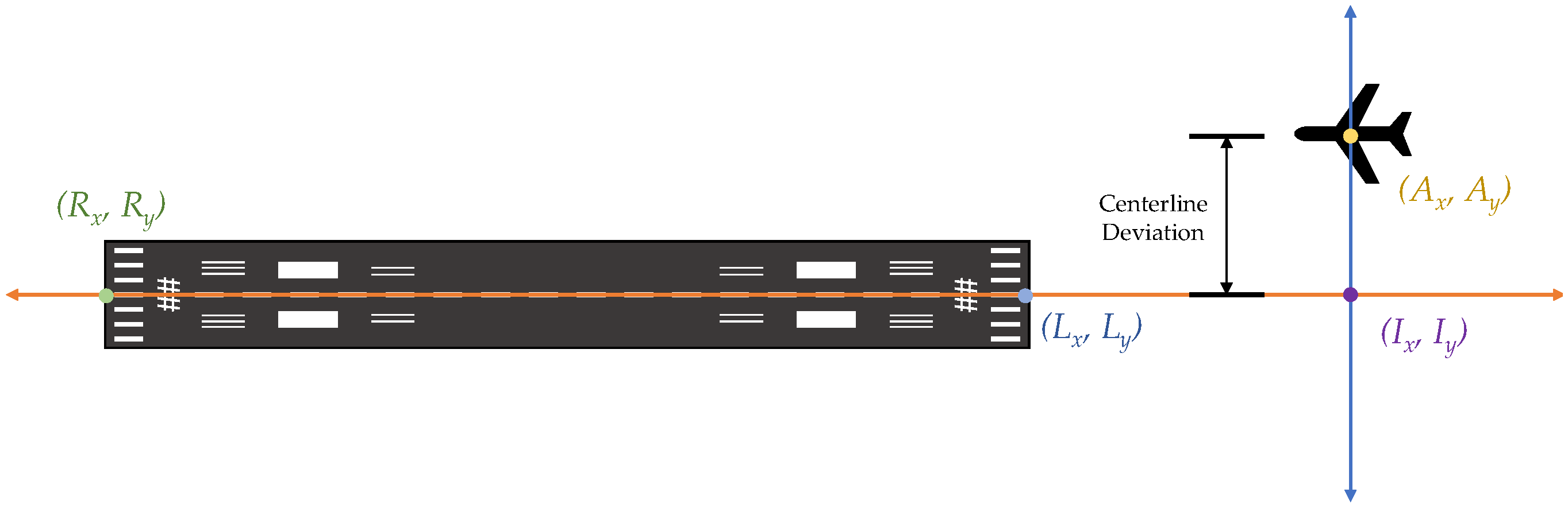
The centerline deviation was calculated by determining the shortest distance between the airplane and an extended centerline from the runway. This calculation was performed using coordinate geometry on a Cartesian coordinate plane. Figure 3 displays a visualization of the points and lines that were applied to calculate the centerline deviation. First, the equation of the runway centerline was determined. Equation (1) was applied to determine the runway centerline slope ($m_{runway}$) and Equation (2) was applied to determine the y-intercept ($y_{runway}$). $(L_x,L_y)$ and $(R_x,R_y)$ represent the positions of each end of the runway on which the aircraft intends to land in UTM coordinates.

$$m_{runway}=\frac{R_y-L_y}{R_x-L_x}$$

(1)

$$y_{runway}=L_y-m_{runway}·L_x$$

(2)

Next, the slope ($m_{perpendicular}$) and y-intercept ($y_{perpendicular}$) of the perpendicular line to the extended centerline that passed through the aircraft position were determined by applying Equations (3) and (4), where $(A_x,A_y)$ represents the position of the aircraft in UTM coordinates.

$$m_{perpendicular}=-1·\frac{1}{m_{runway}}$$

(3)

$$y_{perpendicular}=A_y-m_{perpendicular}·A_x$$

(4)

Finally, the position $(I_x,I_y)$, where the extended centerline intersected the perpendicular line that passed through the aircraft, was determined using Equations (5) and (6).

$$I_x=\frac{y_{runway}-y_{perpendicular}}{m_{perpendicular}-m_{runway}}$$

(5)

$$I_y=m_{runway}·I_x+y_{runway}$$

(6)

The centerline deviation was then calculated as the Euclidean distance between points $(A_x,A_y)$ and $(I_x,I_y)$.

2.4.2. Glide-Slope Deviation and Angle

Aircraft generally follow a standard three-degree glide-slope during approach [23], meaning that the angle between the aircraft and the start of the runway should be three degrees at all points during the approach. Therefore, the glide-slope deviation was calculated by subtracting three from the actual angle that the aircraft made with the start of the runway. Equation (7) was applied to calculate the glide-slope deviation, where $(A_x,A_y)$ is the position of the aircraft in UTM coordinates and $(L_x,L_y)$ is the position of the runway on which the aircraft intends to land in UTM coordinates.

$$glideslopeDeviation=arctan\frac{0.3048\ast altitude}{\sqrt{{(A_x-L_x)}^2+{(A_y-L_y)}^2}}-3$$

(7)

The horizontal plane angle between the aircraft at $(A_x,A_y)$ and the runway at $(L_x,L_y)$ was calculated applying Equation (8), where $cl$ is the centerline deviation calculated applying the methodology from Section 2.4.1.

$$angle=arcsin\frac{cl}{\sqrt{{(A_x-L_x)}^2+{(A_y-L_y)}^2}}$$

(8)

2.4.3. Determination of Landing Runway and Go-Around Runway

Runways are numbered based on the magnetic direction of the runway centerline, and the runway number is one tenth of the direction of the runway in degrees [23]. Therefore, the heading of the aircraft was leveraged to narrow down possible runways.

Table 3. Heading range applied to narrow down landing and go-around runway.

Heading Range	Runways
55–145	10L and 10R
0–55 and 325–360	1L and 1R
145–235	19L and 19R
235–325	28L and 28R

outlines the heading ranges applied to narrow down the runways. After the runways were narrowed down, the centerline deviation, calculated applying the methodology outlined in Section 2.4.1, was applied to select between the “L” (Left) and “R” (Right) options for the runway. Latitude, longitude, and heading values were selected at the minimum altitude prior to the go-around to determine the go-around runway. The latitude, longitude, and heading values at the 1000-feet approach gate were leveraged to determine the landing runway.

2.5. Determination of Other Significant Points

Numpy’s (https://numpy.org/, accessed on 1 September 2021) linear interpolation function was leveraged to determine features at the 1500-feet and 1000-feet approach gates prior to the go-around. Values were interpolated between the first point that the flight reached an altitude below each gate and the previous point. If the altitude at the minimum altitude point prior to the go-around was above the altitude gate, a temporary NaN (not a number) value was recorded for all the features at the gate.

Features at the 1000-feet gate and 2500-feet gate on climb after the go-around were determined similarly to the 1500- and 1000-feet approach gates prior to the go-around. Values were interpolated between the first point after the minimum altitude prior to the go-around that the flight reached an altitude above each gate and the previous point. If the altitude at the minimum altitude point prior to the go-around was above the altitude gate, a temporary NaN value was recorded for all the features at the gate.

The points corresponding to the aircraft’s “maximum altitude hold” following the initiation of the go-around are all points that are within 50 feet inclusive of the maximum height above ground level that the flight reaches after the minimum altitude point prior to the go-around. The maximum altitude that the flight reaches following the initiation of the go-around corresponds to the altitude that the flight holds between the first and second landing. The 50-feet threshold was included for two reasons: (1) on some flights, the altitude during the “maximum altitude hold” fluctuates between two values (i.e., between 5000 feet and 5025 feet), and (2) on some flights, while the majority of the data at the maximum altitude hold are constant (i.e., 5000 feet), one reading might be slightly higher (i.e., 5010 feet). Thus, 50 feet is a sufficient value as flights that fluctuate usually fluctuate between two values 25 feet apart. Moreover, 50 feet is also sufficient to capture flights that have one reading that is slightly higher or lower than the altitude that the aircraft maintains throughout the majority of the “maximum altitude hold”.

The point that corresponds to the start of the maximum altitude hold following the go-around initiation is the first point that the aircraft reaches an altitude within 50 feet of its maximum altitude, as described previously. The half-way point of the maximum altitude hold is the midpoint of all the points at which the aircraft is within 50 feet of its maximum altitude. For example, if the aircraft is within 50 feet of its maximum altitude for 21 points, the 11th point corresponds to the half-way point of maximum altitude hold. If there is an even number of points (n), the $\frac{n}{2}+1$ point is selected. The point at which the aircraft begins descent for its second approach is selected to be the last point at which the aircraft is at an altitude within 50 feet of its maximum altitude hold.

Features at the 1000-feet gate and 500-feet gate on the second approach were determined and extracted similarly to the 1500-feet and 1000-feet approach gates prior to the initiation of the go-around.

2.6. Feature Vector Generation

At every significant point, the features outlined in Table 1 and Table 2 were extracted and arranged as a feature vector. Each row in the feature vector corresponds to a single flight, while each column corresponds to a feature. Two pre-processing steps were conducted prior to clustering. First, all NaN values in the feature vector were replaced with the mean of that column. Second, Scikit-learn’s preprocessing module (https://scikit-learn.org/stable/modules/preprocessing.html, accessed on 1 September 2021) was leveraged to standard scale the feature vector. Standard scaling, also referred to as Z-score normalization [24], ensures that every column of each feature vector has a mean of zero and a standard deviation of one. This acts as a form of normalization, which is a pre-processing step applied before solving most problems with data [24]. This was performed to ensure that a column having values in a larger range or of larger magnitude does not dominate other columns in the data set.

2.7. Clustering

Clustering is an unsupervised machine learning method that attempts to discover structure and patterns in unlabeled data [25]. Clustering algorithms aim to separate data into subsets such that similar data points are grouped together [25]. There are a multitude of clustering algorithms. Clustering algorithms include k-means [26], Agglomerative Hierarchical Clustering [27], density-based spatial clustering of applications with noise (DBSCAN) [28], and Hierarchical DBSCAN (HDBSCAN) [29,30]. These algorithms are also popular in the aviation safety literature [31].

The goal of this analysis was to classify go-around flights into an unknown number of clusters and to identify anomalous go-arounds. Clustering algorithms such as k-means require the user to specify the number of clusters to split the data into. Additionally, k-means is not very effective at dealing with outliers or anomalies and requires that each cluster has a well-defined mean [32]. Agglomerative hierarchical clustering can erroneously split data points into different clusters early and this cannot be corrected later [32]. When agglomerative hierarchical clustering was attempted on the data set during preliminary clustering, it tended to split the data into clusters based on distinct single features and therefore struggled to find meaningful clusters later or failed to consider other features.

DBSCAN and HDBSCAN are clustering techniques that specialize in anomaly detection. Both of these techniques do not require a pre-specified number of clusters. DBSCAN can discover clusters of arbitrary shape based on samples of high density [28]. DBSCAN requires a core distance threshold as a hyperparameter, which impacts the percentage of outliers determined in a data set. In this study, the percentage of flights that were outliers (i.e., anomalies) was unknown, as was the optimal value for the core distance threshold. 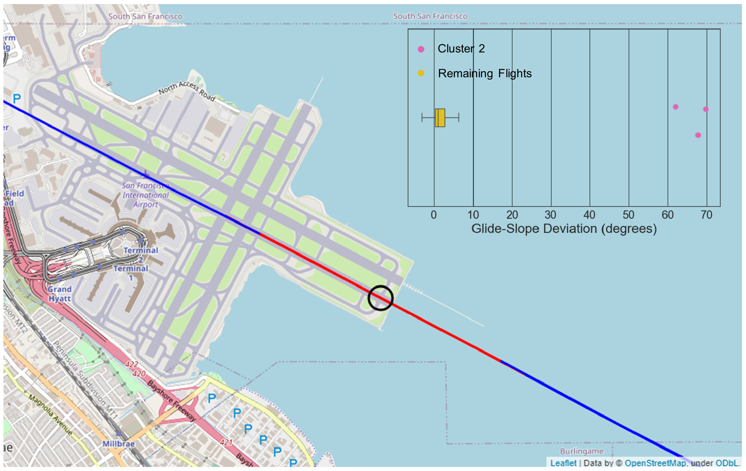HDBSCAN is a density-based clustering algorithm (DBSCAN algorithm core), where the clustering is performed over different DBSCAN core distance thresholds, and it determines the clustering that provides the greatest stability [33]. Additionally, HDBSCAN can identify clusters with differing densities. Consequently, HDBSCAN was able to pick up a second anomalous cluster (discussed later). Recently, HDBSCAN has had success within the aviation literature to analyze approaches [34,35], traffic flows [36], and trajectory clustering [19,20]. Therefore, HDBSCAN was selected for this analysis.

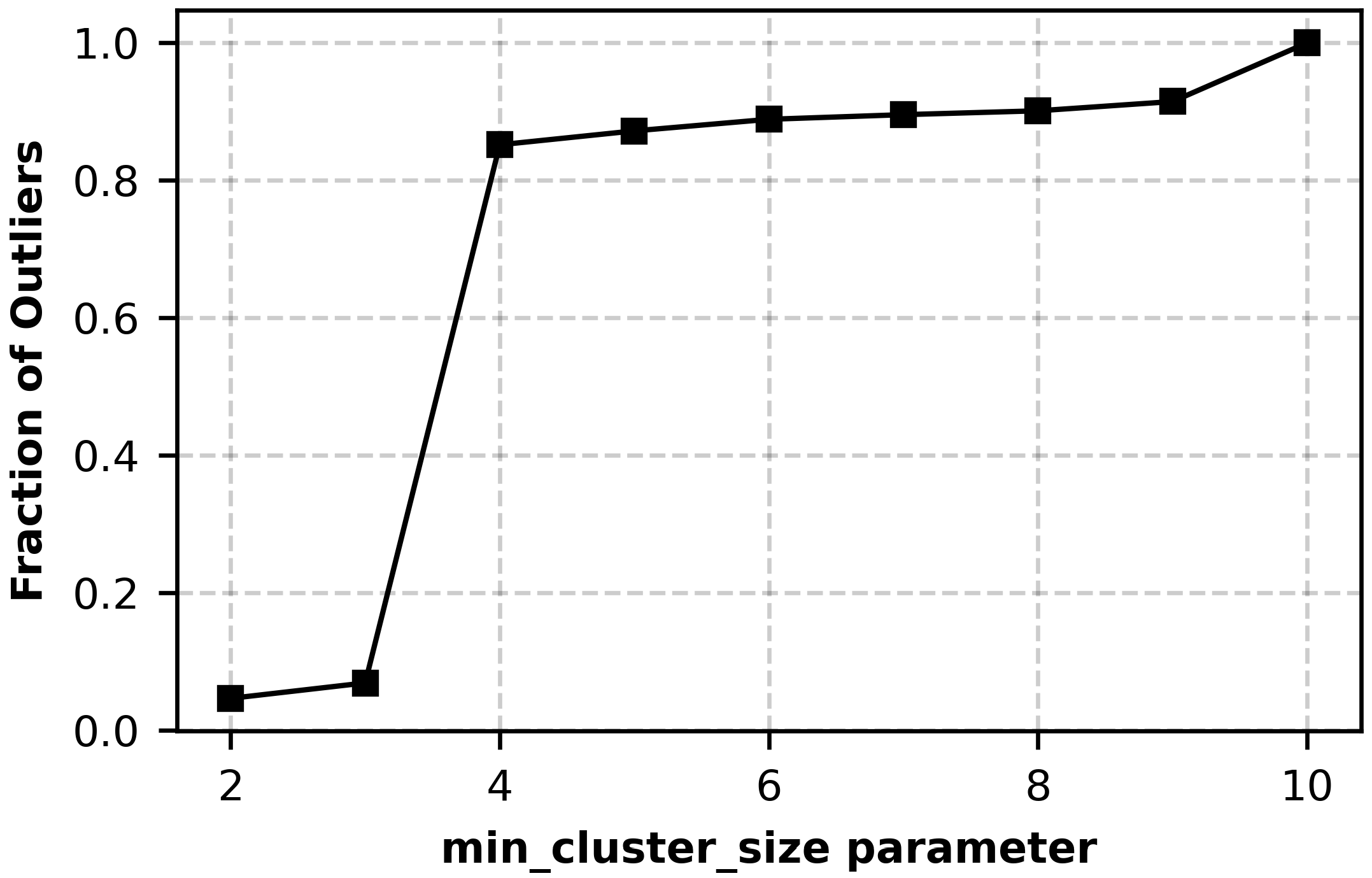
HDBSCAN requires the specification of one hyperparameter: the minimum number of samples required to form a cluster, or minimum cluster size. The minimum cluster size hyperparameter is generally selected based on the total number of data points and the clustering application. As the objective of this study was to analyze trends in go-around flights such that potentially anomalous go-arounds may be detected, clusters with a low number of flights are acceptable because these would indicate operations that are similar to each other, yet sufficiently different than the nominal operations. Therefore, the HDBSCAN algorithm was applied with values of minimum cluster size set to a range from two to ten. Figure 4 displays how the minimum cluster size impacts the percentage of flights detected as outliers. The number of clusters was 2 for minimum cluster size between two and nine and dropped to zero when the minimum cluster size was ten as all points were classified as outliers. A significant increase in flights classified as outliers was observed as the minimum cluster size varied from three to four. Anomalies, by definition, are rare events; thus, they typically make up a small fraction of flights. Therefore, clustering results that detect a small fraction of outliers are preferred. A minimum cluster size value of three provides clustering results with a small fraction of outliers, while still grouping “enough” flights together in each cluster for further analysis of similarities. The HDBSCAN algorithm was implemented using the hdbscan Python library (https://hdbscan.readthedocs.io/en/latest/, accessed on 1 September 2021).

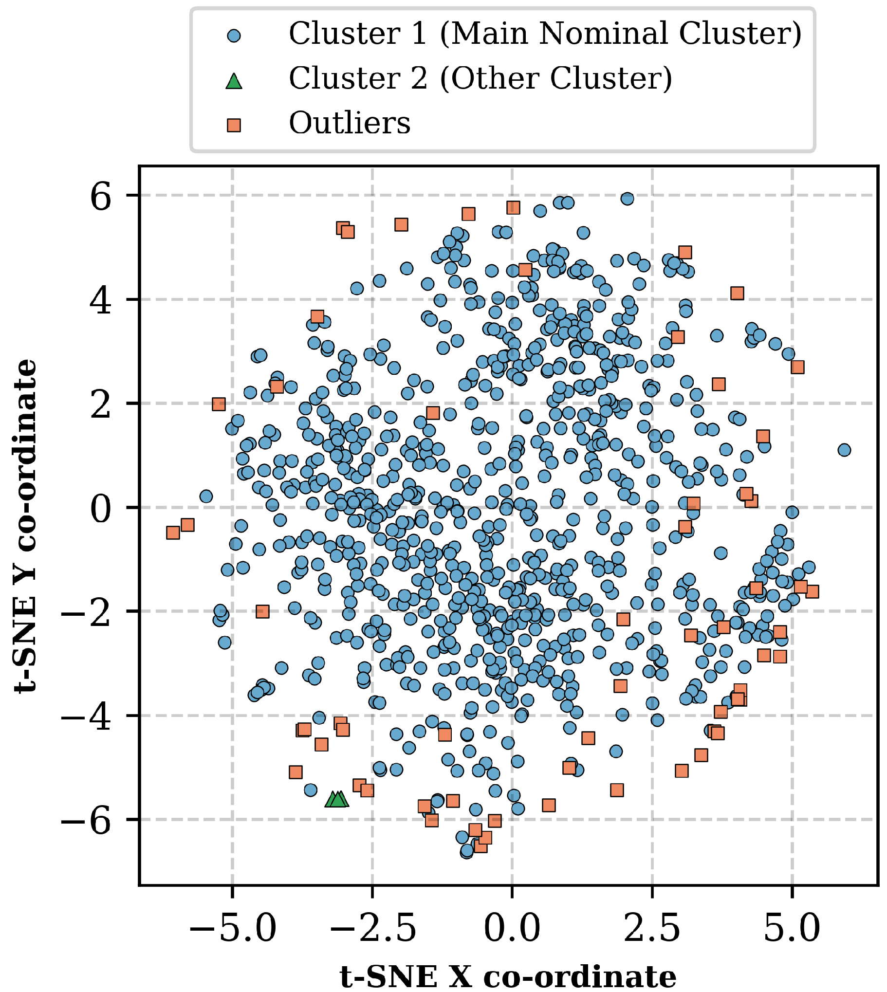
To visualize results of the HDBSCAN clustering, the t-distributed stochastic neighbor embedding (t-SNE) [37] dimensionality reduction technique was applied to reduce the dimensionality of the feature vector to two dimensions. t-SNE is a dimensionality reduction technique that provides insight into both the local structure and global structure of the data and the presence of clusters [37]. t-SNE was implemented leveraging scikit-learn’s manifold module (https://scikit-learn.org/stable/modules/manifold.html, accessed on 1 September 2021).

3. Results and Discussion

In this section, the results of the implementation of the HDBSCAN algorithm are presented. The distribution of features between and within clusters is discussed. Additionally, an in-depth analysis of energy management and outliers is presented.

3.1. Overall Clustering Results

Figure 5 displays the two-dimensional projection of all flights’ feature vectors after applying the t-SNE algorithm, where each flight is colored by the cluster to which it was assigned after applying the HDBSCAN algorithm. The clustering algorithm assigned 826 flights to Cluster 1 (the Major Nominal Cluster), 3 flights to Cluster 2 (the Other Cluster), and identified 61 flights as outliers. The 61 flights that were identified as outliers are displayed in Figure 5 as orange-colored squares. The 826 flights in Cluster 1 are displayed in Figure 5 as blue circles. Finally, the three Cluster 2 flights are displayed in Figure 5 as green triangles. The distinction between the nominal flights and outliers (or anomalous flights) is discussed further in the following sections. First, a deeper examination of the flights placed in Cluster 2, the “Other Cluster”, is presented.

The three flights that were placed in the Other Cluster had an extremely high glide-slope deviation at the minimum altitude prior to the go-around. The median absolute value glide-slope deviation of all go-around flights was 1.17 degrees. The median glide-slope deviation for these three flights was 67.84 degrees. These three flights had a significantly higher glide-slope deviation than the other flights as these flights reached their minimum altitude point either over the runway or close to the runway. Most other flights reached their minimum altitude before the runway. Therefore, the small distance measurement from the end of the runway combined with an altitude significantly higher than ground level resulted in a very high glide-slope deviation measurement. Figure 6 shows an example of one of the flights that was placed into the “Other Cluster”. In this figure, the blue lines represent the trajectory path, the black circle highlights the minimum altitude point, and the red line represents the trajectory path prior to the go-around of the flight when its altitude was less than 500 feet. The box-plot displays the 25th percentile, median, and 75th percentile glide-slope deviation at the minimum altitude point. The whiskers of the box-plot extend out to 1.5 times the inter-quartile range. As Figure 6 indicates, the minimum altitude point was actually above the runway for this particular flight. A possible explanation for the characteristics of these three flights is that the decision to conduct a go-around was made much later than usual, which is supported by the minimum altitude point prior to the go-around being so close to the runway. Although these flights were not classified as outliers by the HDBSCAN algorithm, it is important to acknowledge that these are also anomalous go-arounds. Thus, application of the HDBSCAN algorithm enabled the identification of a group of flights that were all anomalous in the same manner. In the remainder of this section, an analysis of nominal and anomalous go-arounds and possible correlated or causal factors is presented.

3.2. Feature Distribution Discussion

The distribution of features at approach gates were examined to gain an understanding of the overall differences between nominal flights (i.e., Cluster 1) and anomalous flights (i.e., outliers). This may aid in the understanding of causal factors behind nominal and anomalous go-arounds as identified by the algorithm.

Figure 7 and Figure 8 display the distributions of several features at each of the approach gates on the initial approach prior to the go-around and the second approach following the go-around for both the nominal and anomalous flights. The edges of the boxes represent values at the 25th and 75th percentile values and the central line represents the median value. Outliers, which are defined as 1.5 times the inter-quartile range, are not displayed. The whiskers extend out to the minimum/maximum value that is not considered an outlier. In each figure, from left to right, the altitude is lower and, subsequently, the aircraft is closer to the ground or touchdown.

Across all features, the distributions for anomalous flights tend to have a higher inter-quartile range than the distributions of nominal flights. However, comparing the distributions between Figure 7 and Figure 8, the distribution of features for anomalous flights tends to be closer to the nominal flights for the approach following the go-around than the approach prior to the go-around. This indicates that the anomalous flights are more similar to the nominal flights during the second approach, which leads to a successful landing. Examining the first approach prior to the go-around (Figure 7) reveals some interesting trends. At the minimum altitude prior to the go-around, 1000-feet approach gate, and 1500-feet approach gate, anomalous flights have a higher median specific energy and velocity than nominal flights. Additionally, at the 1000-feet approach gate and 1500-feet approach gate, the velocity and specific energy at the third quartile are significantly higher for anomalous flights. This indicates the possibility of anomalous go-arounds having higher energy and, possibly, poor energy management, when compared with the nominal flights. The other examined features are directly related to stable approach criteria. The anomalous flights tend to have a higher magnitude vertical rate (indicated by both the median and quartile values) than the nominal flights at both the approach gates. Under stable approach guidelines, aircraft should maintain a vertical rate magnitude below 1000 feet/minute [1]. At the 1000-feet approach gate, almost all nominal flights are below this value, while over 25% of the anomalous flights have a vertical rate magnitude greater than 1000 feet/minute. Stable approach criteria also require that aircraft are within 1 degree of the glide-slope [1]. At the 1000-feet approach gate, almost all nominal flights are within the 1 degree glide-slope deviation, while over 25% of the anomalous flights have a glide-slope deviation greater than one degree. Similar distributions are observed for both the runway angle and centerline deviation parameters, where the anomalous flights tend to be further deviated than the nominal flights. This indicates that approach stability is correlated with the classification of the go-around as nominal or anomalous, but not necessarily with whether a go-around is conducted or not (all flights in our set are go-arounds, yet many had a stable approach).

Interestingly, considering Figure 7 and Figure 8, in the distributions of features and metrics in the approach prior to go-around, the nominal and anomalous flights deviate from and remain distinct from each other. On the other hand, after the go-around, the distinction between the two sets is smaller and diminishes closer to actual touchdown.

3.3. Energy Management Discussion

Proper energy management plays a significant role in the safety and success of aviation approaches [38,39]. Puranik et al. [40] completed a survey of the existing literature on energy management in aviation operations and identified the energy metrics that are most relevant. Puranik et al. indicated that energy states for an aircraft can be used as an objective currency to evaluate various safety-critical conditions during flight [40]. The definition and utilization of energy metrics is common within the aviation literature, particularly in anomaly detection using ADS-B data. Corrado et al. [20] introduced the concept of energy anomalies in ADS-B trajectory data, which are detected as those trajectories whose energy metrics do not conform to standard operations. While Corrado et al. did not consider go-arounds in their work, it follows from the previous sub-section that energy metrics and energy management do play a significant role in the analysis of go-arounds. For instance, Blajev et al. discovered that high or low aircraft energy states can “make the safe execution of go-arounds less likely” [2]. The feature distribution analysis from the previous sub-section indicated the possibility of energy management playing a role in the identification and classification of the go-arounds. Therefore, the energy states of the nominal and anomalous flights throughout the entire go-around were examined here in depth.

Figure 9 and Figure 10 display plots of the specific total energy and specific kinetic energy of nominal and anomalous flights at various cumulative ground track distances as the shaded regions. The 25th and 75th percentile values for each distribution are plotted. Figure 9 and Figure 10 directly compare the nominal and anomalous flights for the first approach prior to the go-around and the second approach following the go-around, respectively.

For the first approach prior to the go-around, the ground track distance is the cumulative ground track distance of the aircraft with respect to the minimum altitude point prior to the go-around plus the distance of the aircraft from the runway at the minimum altitude prior to the go-around. For the second approach, the ground track distance is the cumulative ground track distance of the aircraft with respect to the landing point, as explained in Section 2.1. A maximum cumulative ground track distance of 30 nautical miles was chosen for the second approach such that energy states during the go-around trajectory could be captured and compared.

Figure 9 indicates that the 25th percentile values for anomalous flights at each of the cumulative ground track distances are almost equal to, or only slightly higher than, the nominal flights. However, both the specific total energy and specific kinetic energy states at the 75th percentile values of anomalous flights are significantly higher than nominal flights. This implies that the anomalous flights tend to have significantly higher energy states throughout the entire approach prior to the go-around. However, Figure 10 indicates significant overlap between energy states at the 25th and 75th percentile values for both nominal and anomalous flights on the second approach following the go-around. This supports earlier observations that the anomalous flights are similar to the nominal flights for the second approach following the go-around.

Figure 11 compares the energy states of the aircraft between the first approach prior to the go-around and the second approach following the go-around by separating the nominal and anomalous flights. This allows comparison of the different classes of flights with themselves on the second landing attempt. The plot again shows the 25th and 75th percentile values. However, for an accurate comparison between the first approach and second approach, the specific kinetic energy was plotted at every 100-feet altitude gate between 500 feet and 4000 feet. It is evident that flights tend to have higher energy states on the first approach prior to the go-around than the second approach after the go-around (particularly for the anomalous class). The flights that were categorized as anomalous also have a significantly higher difference in the 25th and 75th percentile specific kinetic energy between the two landing attempts than the nominal flights. Since all these flights completed a successful landing following the second approach, the second approach can be considered a “normal” approach. Therefore, these plots indicate that the energy states for nominal flights on the approach prior to the go-around were closer to what they would be on a “normal” approach, while the energy states for anomalous flights on the approach prior to the go-around were significantly higher than they would be on a “normal” approach. Therefore, these observations indicate that the anomalous go-arounds could have a closer relationship with safety margins than the nominal go-arounds, and this warrants further investigation in future work.

Figure 12 shows a two-dimensional density contour plot of the specific potential energy versus specific kinetic energy of all the nominal flights during all descent phases (vertical rate below −100 ft/min). The specific potential energy and specific kinetic energy of one anomalous flight are overlaid on top of the density contour plot. The points in red correspond to the first approach prior to the go-around and the orange points correspond to the second approach after the go-around. This plot provides a good visualization of the earlier observations related to some anomalous flights following an energy trajectory that is significantly outside the bounds of the energy states of nominal flights during the first approach. However, these anomalous flights tend to have comparable energy states that are on par with nominal flights on their second approach.

4. Conclusions

This paper presented a novel methodology to classify and analyze go-arounds. Go-around flights were first detected from the OpenSky Network’s historical database of approaches into San Francisco International Airport in 2019. An extensive literature search was conducted to identify and select significant points during the execution of a go-around and significant features at these points. The identified features were extracted at each point for the analysis of these go-around flights.

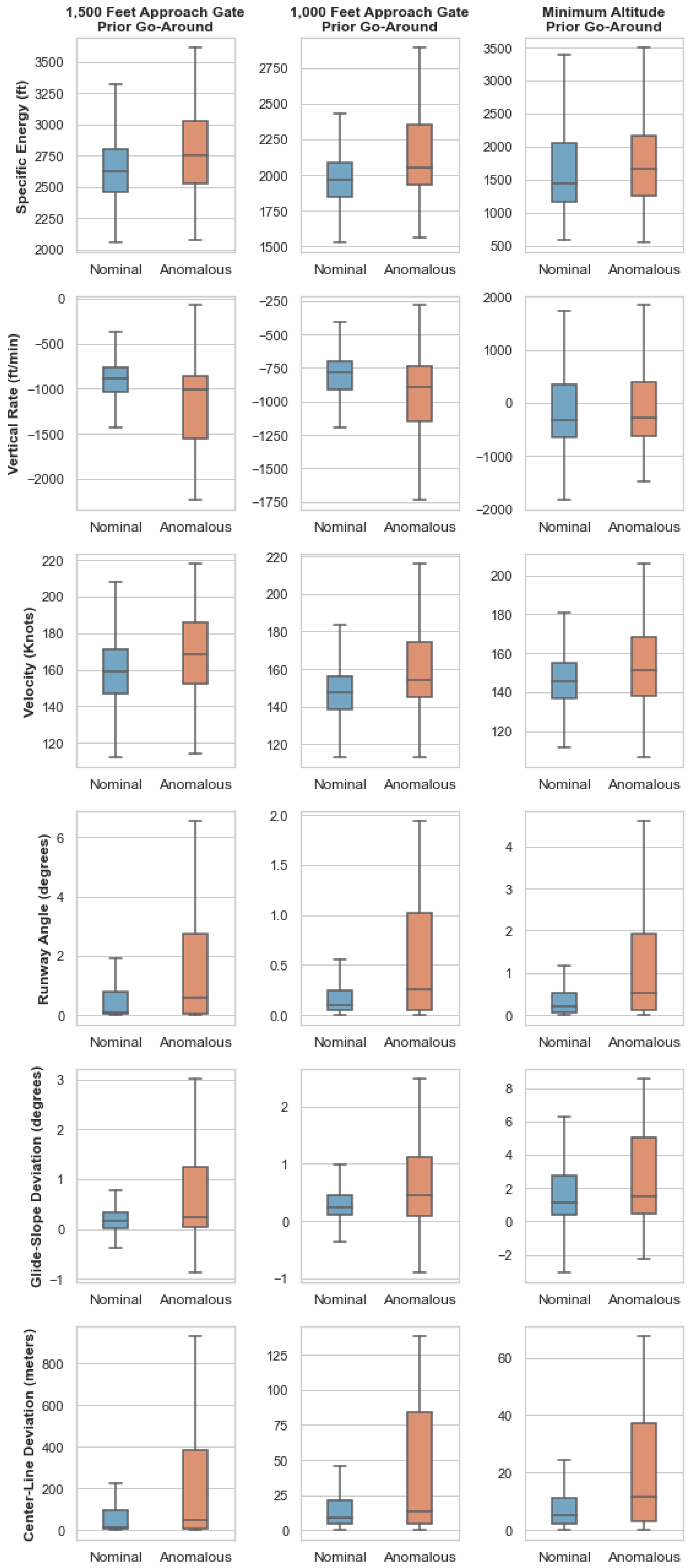
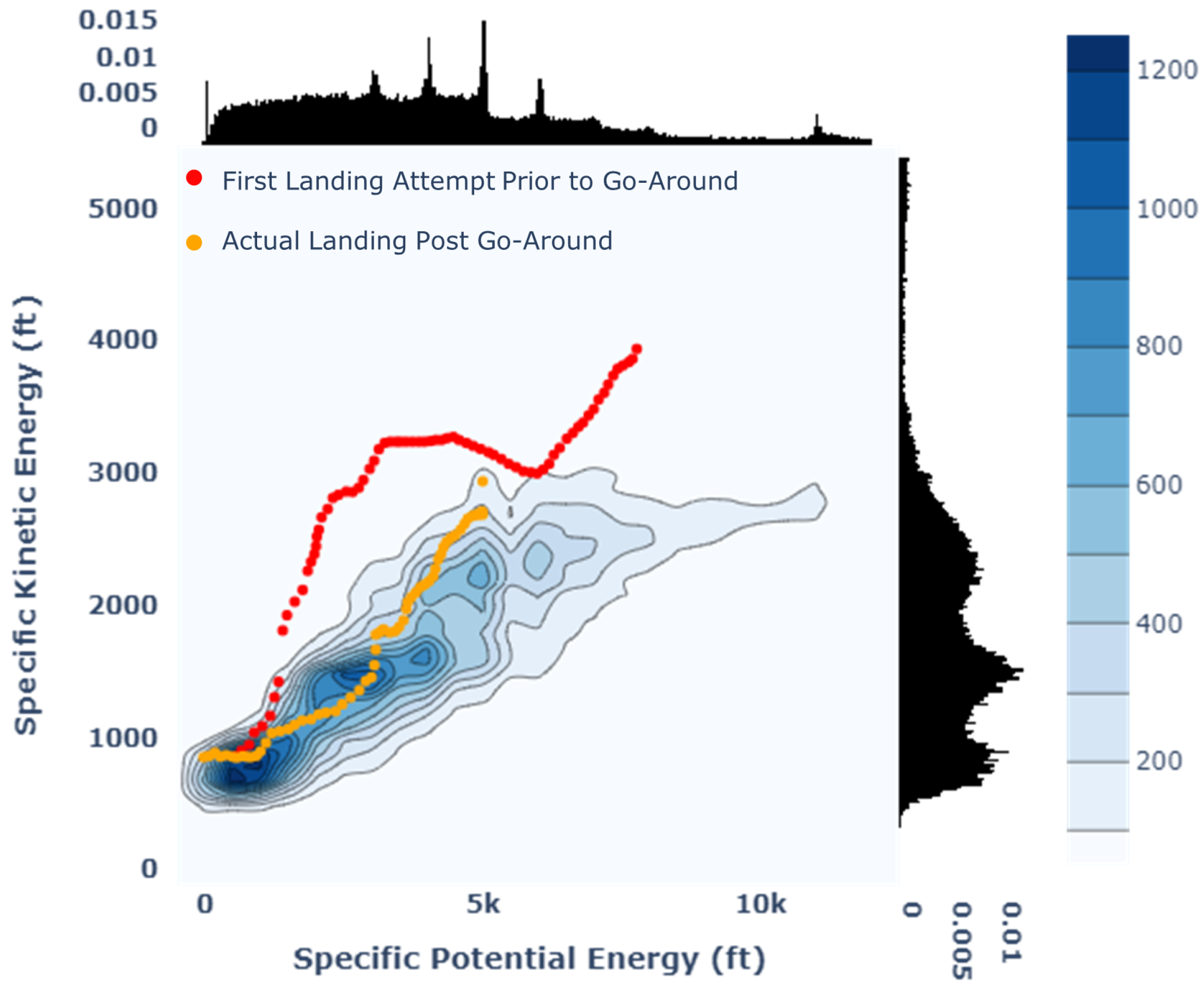
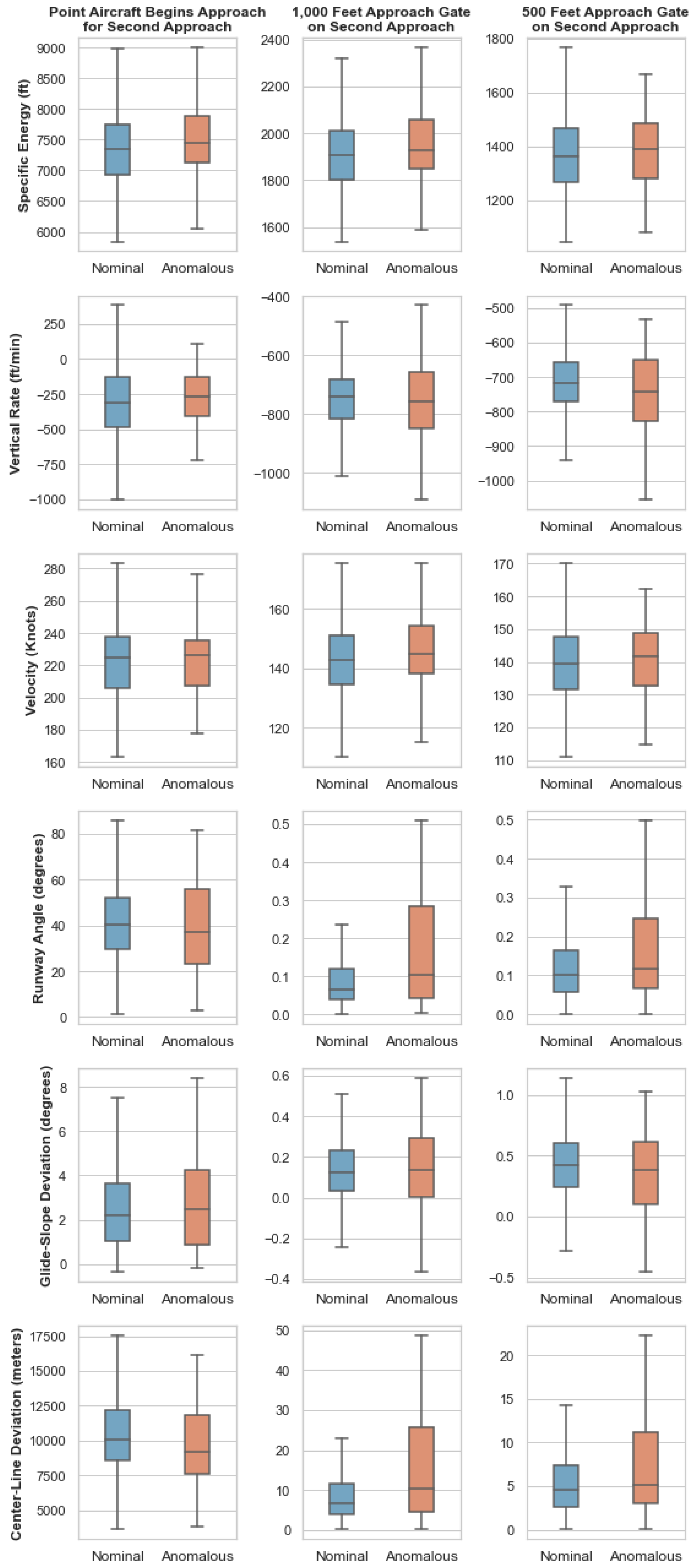
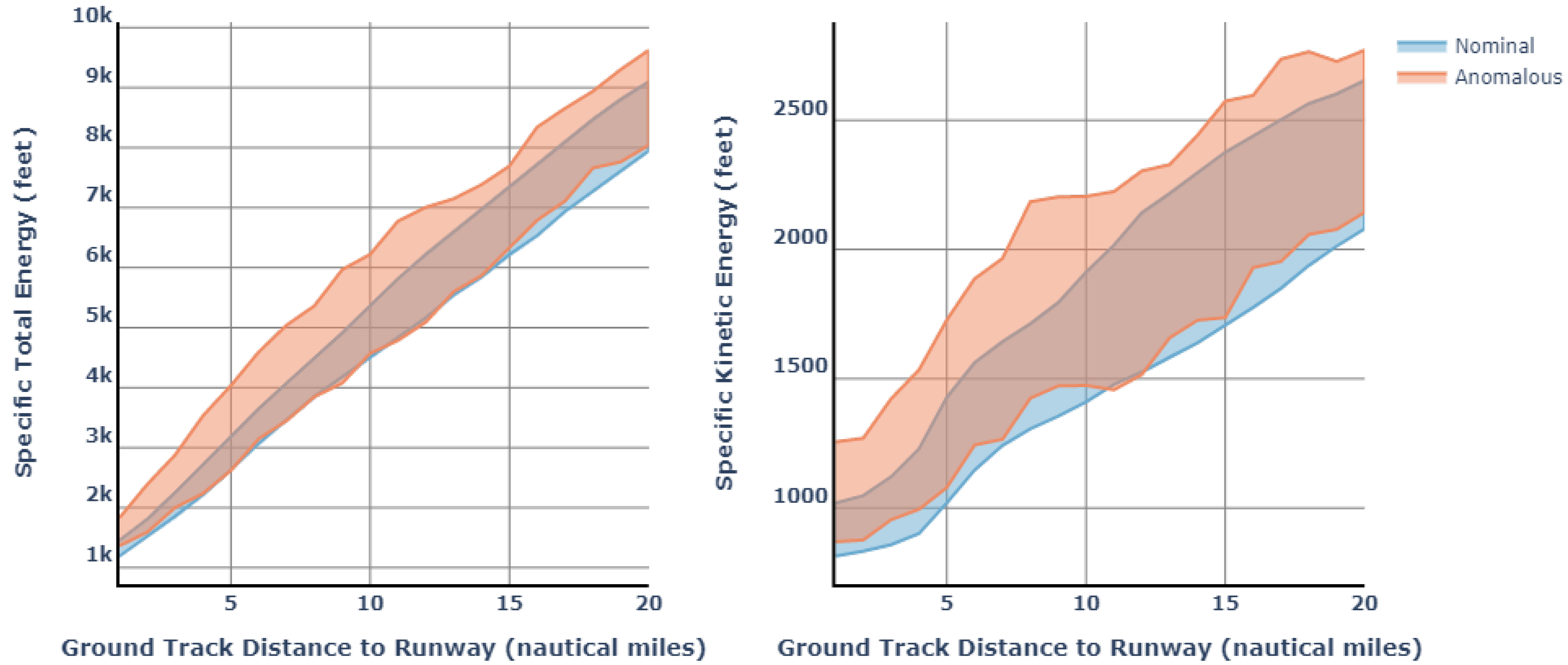
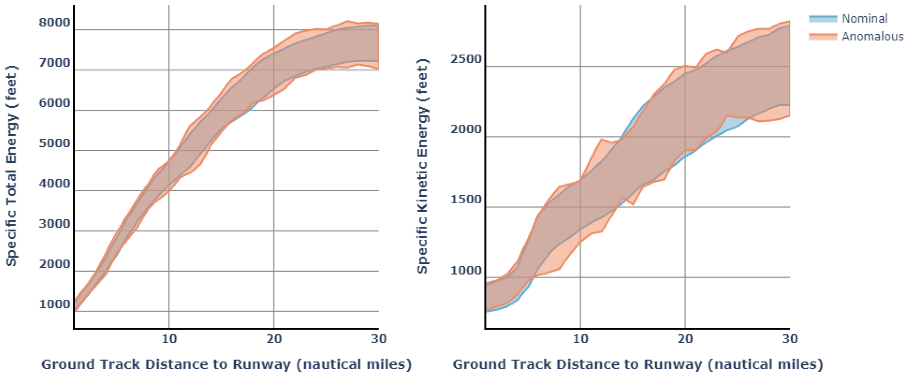
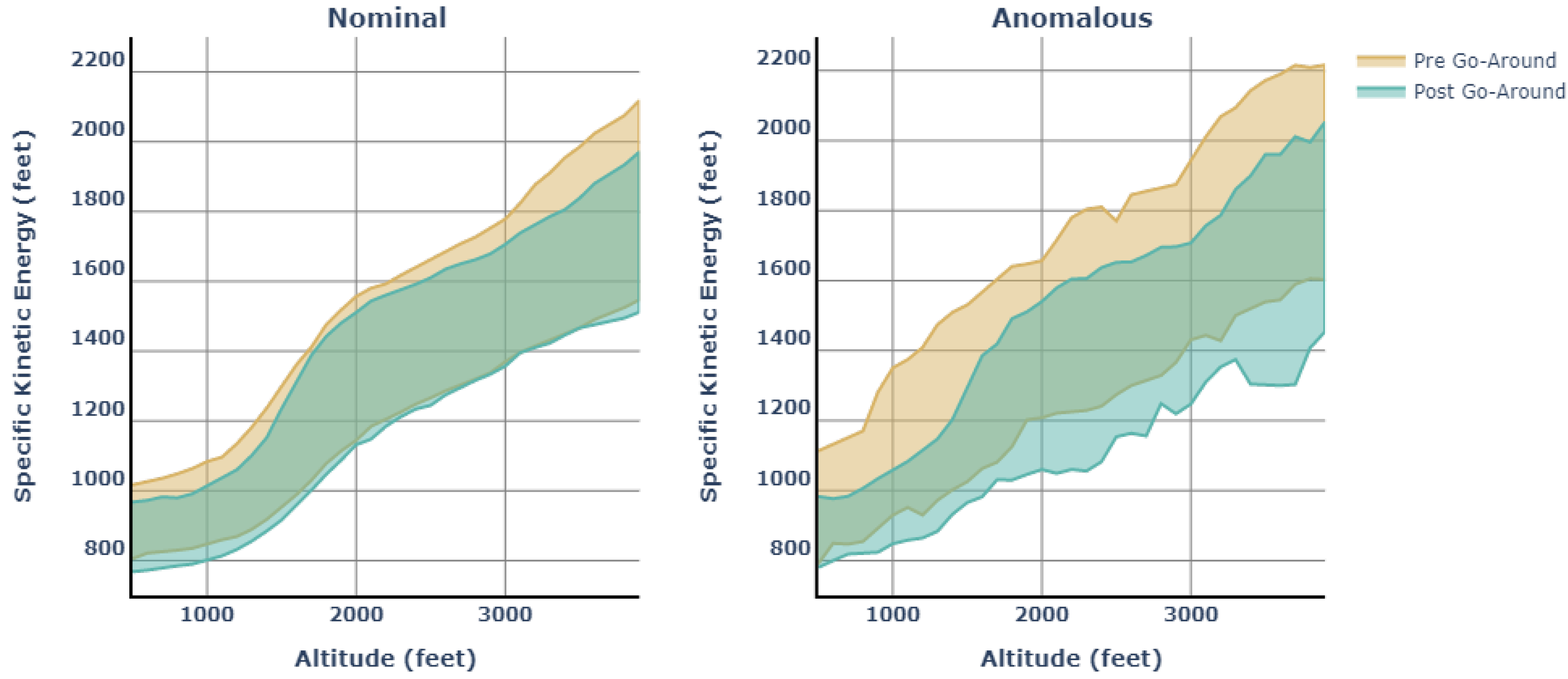
Go-arounds were classified, by applying the HDBSCAN clustering algorithm, into a nominal cluster, anomalous cluster, and another cluster that consisted of flights that conducted a go-around much later than normal. Further analysis was conducted on each category of go-arounds. Flights that were categorized as anomalous tended to have higher deviations from standard procedures or nominal flights on the initial approach prior to the go-around. Furthermore, a comparison of the energy states of the nominal and anomalous go-arounds indicated much higher energy states for anomalous go-arounds on the initial landing attempt.

Limitations of the methodology stem from limitations of the data utilized. For example, reference speed, which is utilized in stable approach determination, could not be calculated as factors such as aircraft weight would have had to be approximated. There were many references made throughout the paper to stable approach criteria. Consequently, due to these limitations, flights in this paper were not explicitly marked as stable or unstable. Additional aircraft data, such as aircraft attitude, which are considered important during the execution of a go-around, and other features available through Flight Operational Quality Assurance (FOQA) data, would have been helpful to gain better insights into aspects of nominal and anomalous go-arounds. A key facet of this work is the demonstration of the use of widely available open-source ADS-B trajectory data for go-around research and classification.

Given that go-arounds are a necessary procedure during landing operations, this work aids in understanding aspects that lead to anomalous go-arounds. The methodology discussed in this paper could be utilized by subject matter experts to identify anomalous go-arounds and to examine the detected go-arounds for further analysis specifically related to improper energy management. In future work, further analysis of the entire trajectory of anomalous go-arounds will be conducted. Additionally, correlations between external factors such as weather, air traffic control constraints, time, etc., and these outliers will also be examined.