Article

Unsupervised Anomaly Detection in Flight Data Using Convolutional Variational Auto-Encoder

1
Data Sciences Group, NASA Ames Research Center, USRA, Moffett Field, CA 94035, USA
2
Data Sciences Group, NASA Ames Research Center, KBR Inc., Moffett Field, CA 94035, USA
*
Author to whom correspondence should be addressed.
Aerospace 2020, 7(8), 115; https://doi.org/10.3390/aerospace7080115
Submission received: 7 July 2020 / Revised: 31 July 2020 / Accepted: 6 August 2020 / Published: 8 August 2020
(This article belongs to the Special Issue Machine Learning Applications in Aviation Safety)

Abstract

:
The modern National Airspace System (NAS) is an extremely safe system and the aviation industry has experienced a steady decrease in fatalities over the years. This is in part due the airlines, manufacturers, FAA, and research institutions all continually working to improve the safety of the operations. However, the current approach for identifying vulnerabilities in NAS operations leverages domain expertise using knowledge about how the system should behave within the expected tolerances to known safety margins. This approach works well when the system has a well-defined operating condition. However, the operations in the NAS can be highly complex with various nuances that render it difficult to assess risk based on pre-defined safety vulnerabilities. Moreover, state-of-the-art machine learning models that are developed for event detection in aerospace data usually rely on supervised learning. However, in many real-world problems, such as flight safety, creating labels for the data requires specialized expertise that is time consuming and therefore largely impractical. To address this challenge, we develop a Convolutional Variational Auto-Encoder (CVAE), an unsupervised deep generative model for anomaly detection in high-dimensional time-series data. Validating on Yahoo’s benchmark data as well as a case study of identifying anomalies in commercial flights’ take-offs, we show that CVAE outperforms both classic and deep learning-based approaches in precision and recall of detecting anomalies.

1. Introduction

As the National Airspace System (NAS) has evolved over the years, it has been able to accommodate commercial passenger demand while maintaining exceptional levels of safety. According to the National Transportation Safety Board (NTSB), the accident rate per 100,000 flight hours has been cut in half since 2000—from 0.306 to 0.156 in 2018 [1]. While the number of passenger enplanements has increased 20% from 706 million in 2009 to 851 million in 2017, the number of departures has decreased 5% from 9.7 million to 9.3 million over the same period [2]. This trend has resulted in a historically high passenger load factor of 82.3% in 2017 [3]. While the number of flights has remained relatively flat, the passenger load factor is approaching saturation and will result in more departing flights in the future. To remain at this historically low level of accidents per year, the NAS will need to innovate and proactively identify operationally significant safety events that are currently not being tracked. The FAA outlines proactive and reactive hazard and risk reduction under the auspices of safety risk management. This process is described within Section 2.1.3 of the 2019 Safety Management System Manual [4]. Identifying vulnerabilities or hazards is a key step in the process where machine learning can provide assistance and eventually lead to implementation of risk mitigation in the form of revising safety requirements to address the newly identified vulnerability. Although any vulnerability discovery method needs to be cognizant of high false positive rates when determining requirements for the operationalization of the system, missed detection also carry a high cost to safety and should be factored into the planned operations by the stakeholders.
Identifying situations where unknown risk or vulnerabilities exist is not a trivial problem. Much of the knowledge of adverse events comes from after-the-fact analysis using forensic investigations to determine the root cause of an incident or accident such as the manual process that NTSB uses when investigating accidents [5]. In 2007, the Federal Aviation Administration (FAA) partnered with MITRE Corp to develop the Aviation Safety Information and Sharing (ASIAS) system. This system archives air carrier flight data and promotes proactive analytics which could identify safety risks in the NAS before they lead to a significant incident or accident. One aspect of the program acts as a repository for Flight Operational Quality Assurance (FOQA) data. These data are comprised primarily of 1 Hz recordings for each flight. These recordings cover a variety of systems, including the state and orientation of the aircraft, positions and inputs of the control surfaces, engine parameters, and auto pilot modes’ corresponding states. The data are acquired in real time on-board the aircraft and downloaded by the airline once the aircraft has reached the destination gate. These time series are analyzed by domain experts, who derive threshold-based algorithms post-flight to flag known events. Events that are deemed to be of operational significance are then determined by the airline. These events are monitored over time to determine emerging trends or quantify safety improvements. The ASIAS program acts as an independent broker that does not have regulatory authority and can provide each airline a centralized assessment of their safety performance compared to other similar airlines in a de-identified context. However, in 2013, an Inspector General’s (IG) report [6] found that the “system lacked advanced analytical capabilities” and tasked the FAA to further improve the system. In October 2019, the IG began a follow-up review to assess the progress of ASIAS in addressing the IG’s 2013 recommendations [7].
Improving the ability to identify emerging vulnerabilities in current operations helps to increase awareness of new threats. Proactively addressing safety requires developing, testing, and validating new approaches that can process and model large amounts of historically recorded heterogeneous data. Such data describe the operations of millions of flights over multiple years and covers various diverse regions in the NAS. Data science and machine learning approaches have the potential to automatically identify anomalous events in these observed data. However, the events identified still need to be reviewed and assessed by subject matter experts familiar with the procedures in order to better understand how operations are carried out, and their safety implications. Possible vulnerabilities can then be addressed by mitigating the contributing factors with proper countermeasures. These may include improved pilot/controller training or developing automation safety processes, which, when in place, help to avoid states that result in an increased likelihood of an incident or accident that may result in damage to the aircraft, injury, or loss of life. For example, as the Boeing 737 MAX went into service, comparisons with existing 737 models’ operations may have highlighted significant differences due to the Maneuvering Characteristics Augmentation System (MCAS). This early identification of unexpected behaviors during a critical phase of flight, shortly after takeoff, in the 737 MAX might have yielded insights about the vulnerabilities of the MCAS. Having this information available to operators, manufacturers, and regulators could have led to actions that might have prevented the Lion Air Flight 610 and Ethiopian Airlines Flight 302 accidents [8]. However, it is important that any decision support tool has both low false positive (false alarm) and false negative (missed anomalies) rates, in order to ensure that the user has trust in the system and takes appropriate actions.
In order to improve and automate identification of these vulnerabilities, we have developed an unsupervised machine learning algorithm that constructs models based on observed operations and identifies operationally significant safety anomalies. This algorithm is demonstrated to improve performance as compared to existing anomaly detection methods used in this domain. The paper is organized as follows: In Section 2, we cover related work. In Section 3, a description of the proposed method is discussed with a background on existing concepts used to construct the method and attention to the innovative contribution we have made. In Section 4, we demonstrate the model’s performance on the publicly available Yahoo! benchmark time series data and real world FOQA data and compare performance with several classic (K-Means and One-Class Support Vector Machine) and deep learning-based (Auto-Encoder and Generative Adversarial Networks) anomaly detection methods. Finally, in Section 5, we discuss our conclusions and future work.

2. Related Work

The standard anomaly detection technique in aerospace data is exceedance detection. This technique compares specific parameters against pre-defined thresholds, which are identified based on domain knowledge. The exceedance analysis is described in the FAA document on the FOQA program [9] and implemented in flight data monitoring software used by airlines and aviation equipment manufacturers (e.g., eFOQA from GE or AirFase from Teledyne). The exceedance detection method performs well on known issues, but is incapable of identifying unknown risks and vulnerabilities.
In order to identify unknown risks and vulnerabilities, we need to go beyond simplistic rule-based thresholding approaches. Recent advancements in the field of machine learning have shed light on their application for identifying anomalies in aviation data. Generally, machine learning approaches used for anomaly detection can be categorized into supervised and unsupervised methods, with the presence of labels a key differentiator between the two. Lee et al. [10] developed an interpretable framework to visualize and process FOQA data and to identify safety anomalies in the data using several supervised machine learning classification methods. Janakiraman [11] also developed a deep multiple instance learning approach for supervised classification of adverse events to identify precursors in FOQA data. However, the difficulty of obtaining labels even for known anomalies in aerospace data makes an unsupervised approach often the only feasible option, and such an approach is the focus of this article. Unsupervised machine learning algorithms used for anomaly detection in aerospace data include proximity-based methods (nearest neighbors and clustering-based), support vector machines (SVM) and, more recently, deep learning methods.
Bay and Schwabacher [12] is among the proximity-based approaches that develop an algorithm which defines an anomaly as a point in feature space whose nearest neighbors are far from it. This algorithm was applied to detect anomalies in Space Shuttle main engines. Another line of work relies on clustering methods, such as the Sequence Miner algorithm for discrete flight parameters (cockpit switch flips) [13] and the Inductive Monitoring System (IMS) [14] for continuous parameters. These studies rely on identifying “normal” regions in the feature space, and then computing an anomaly score by measuring the distance between the observed data and these regions. In the investigation of the Space Shuttle Columbia disaster, IMS has been applied to temperature-sensor data of the Shuttle’s left wing, detecting in retrospect the damage from the foam impact [15]. The ClusterAD-Flight method [16] transforms FOQA time series data into high-dimensional vectors, making different flights comparable by sampling each flight parameter at fixed temporal or distance-based intervals starting from an anchoring event (e.g., time from takeoff or distance from touchdown) with subsequent clustering using the density-based spatial clustering algorithm.
One-class SVMs (OC-SVM) are a popular unsupervised approach for anomaly detection. A OC-SVM constructs an optimal hyperplane separating normal data in the high dimensional kernel space by maximizing the margin between the origin and the hyperplane. This approach has been developed for anomaly detection in aviation data as well [17]. A major challenge in implementing OC-SVMs is the computational complexity of the kernel building step, which is quadratic with respect to the number of training examples.
Anomaly detection using deep neural networks has caught much attention recently. This reflects a rising trend in the popularity of deep learning due to its flexibility and scalability. One of these approaches is the Autoencoder (AE) [18], which is a feed-forward multi-layer neural network trained to copy its input to its output by minimizing the reconstruction error. It could be viewed as a nonlinear generalization of Principal Component Analysis (PCA). An AE uses a multi-layer encoder network to transform the high-dimensional data into a low-dimensional latent space, and a decoder network to recover the input data from the latent space [18]. Anomaly detection with an AE uses the reconstruction error as an anomaly score. Reddy et al. [19] applied an AE to raw time series data from multiple flight sensors by using sliding overlapping time windows to form input vectors (a much earlier example of applying an AE to spacecraft data can be found in [20]). Zhou et al. [21] implement an AE with regularization term (called “robust AE”) to eliminate outliers in case of lacking clean training data. The main difficulty of applying autoencoders is the choice of the right “degree of compression”, i.e., the dimensionality of the latent space and finding its right trade-off between fit to the data and model flexibility.
Work by Kingma and Welling [22] and Rezende et al. [23] bridged recent advancements in deep learning with variational inference by introducing the concept of a Variational Auto-Encoder (VAE) (see details in Section 3 of this paper). VAEs are deep generative models that are used for various applications, with anomaly detection becoming increasingly popular. An and Cho [24] proposed an anomaly detection method based on a VAE with the anomaly score as a Monte Carlo estimate of the reconstruction log-likelihood, which they called “reconstruction probability”. Haowen Xu et al. [25] used this approach for detecting anomalies in univariate time series representing seasonal key performance indicators in web applications, with the input vector formed by applying a sliding time window.
Generative adversarial networks (GANs) are another type of deep generative models that have increased in popularity for use in anomaly detection. For example, Zenati et al. [26] developed an efficient anomaly detection approach based on Bidirectional GANs [27,28], which we also use for benchmarking performance of our proposed model. Following the success of using deep Recurrent Neural Networks (RNN) for machine learning applications with sequential data, approaches of using VAEs with RNNs for anomaly detection in time series have been actively explored as well. They usually use Long Short-Term Memory (LSTM) constructs for VAE encoder and decoder networks to handle temporal dependencies in data [29,30,31,32,33]. The LSTM-VAE approach has also been applied for anomaly detection in telemetry data from the Soil Moisture Active Passive (SMAP) satellite and the Mars Curiosity rover [34]. However, VAEs based on the RNN architecture are computationally expensive to train for high-dimensional time series and may overlook local temporal dependencies.

3. Method

Unsupervised detection of anomalous patterns in high-dimensional heterogeneous time series such as FOQA data are an extremely challenging task. The model trained for this task must be able to capture complex patterns in correlated heterogeneous data in order to identify anomalous trends. In this section, we outline our proposed model, the Convolutional Variational Auto-Encoder (CVAE), which is specifically designed for anomaly detection in high-dimensional heterogeneous time series data. The CVAE model is comprised of two main parts: (1) an encoder, which maps the original data space (X) into a compressed low-dimensional latent space (Z) and (2) a decoder, which reconstructs the original data by sampling from the low-dimensional latent space. As illustrated in Figure 1, given all data entries, CVAE adapts the rate of fitting the model to the unbalanced training data, which contains a significantly lower number of anomalous than nominal examples. In this process, CVAE is able to successfully learn the optimal mapping of the nominal data to the latent space and to reconstruct them (i.e., x ^ nominal ) with small reconstruction error, i.e., | | x nominal x ^ nominal | | 2 2 . However, for anomalous data, the mapping to the latent space is not optimized and hence results in significantly higher reconstruction error. In this way, the reconstruction error can be used as a metric to identify anomalies. It should be noted that the level of fitting to the training data needs careful consideration, as CVAE can also fit to the anomalous data. If this is the case, the reconstruction error for anomalies can be as low as the error for nominal data, which is an undesirable outcome. We take inspiration from [35] to control the levels of fitting to nominal and anomalous training data by introducing a hyperparameter in the loss function of the machine learning model. We start with summarizing a basic understanding of variational inference and VAEs, and then explain the proposed model in detail.

3.1. Variational Inference

Let us assume the following problem: given the original data, x X , and the latent variables, z Z , the goal is to estimate the conditional density of the posterior of the latent variables, i.e., p ( z x ) , which can be computed using the Bayes rule,
p ( z x ) = p ( z , x ) p ( x )
The denominator in the above equation is called the evidence. In order to calculate the evidence, one needs to compute the following integral:
p ( x ) = z p ( z , x ) d z
However, computing this integral is usually intractable. In order to approximate the posterior of the latent variables, i.e., p ( z x ) , two paradigms are used: (1) Markov Chain Monte Carlo (MCMC), which uses sampling across an ergodic Markov chain on the latent variable z whose stationary distribution is the posterior p ( z x ) ; and (2) variational inference (VI), which uses optimization instead of sampling to approximate the posterior by minimizing the Kullback–Leibler (KL) divergence between the estimated posterior and the exact one,
f * ( z ) = argmin f F KL f ( z ) | | p ( z x )
where f ( z ) is an arbitrary function defined over variable z, F is the domain of all possible candidates for function f, and f * ( z ) is the function that achieves the minimum KL divergence with respect to the posterior distribution p ( z x ) . While MCMC provides guarantees of producing samples from the exact posterior distribution, it is computationally expensive—especially when datasets are large and models are complex. VI, on the other hand, is faster and applicable to complex problems, while sacrificing the guarantee of convergence to the exact posterior. However, the objective defined in Equation (3) is not tractable to compute as it requires computing the log of the evidence, i.e., log p ( x ) . To see this, we need to extend the definition of the KL divergence:
KL f ( z ) | | p ( z x ) = f ( z ) log f ( z ) p ( z x ) d z = E f ( z ) [ log f ( z ) ] E f ( z ) [ log p ( z x ) ] = E f ( z ) [ log f ( z ) ] E f ( z ) [ log p ( z , x ) ] + log p ( x )
Due to the dependence of the KL divergence on the evidence (i.e., log p ( x ) ), we cannot compute it. As a result, VI relies on optimizing an alternative objective, which is called the evidence lower bound (ELBO),
ELBO ( f ) = E f ( z ) [ log p ( z , x ) ] E f ( z ) [ log f ( z ) ]
As noted, the ELBO is the negative KL divergence (defined in Equation (4)) plus log p ( x ) , which is a constant when we take the expectation with respect to f ( z ) . As a result, maximizing the ELBO is equivalent to minimizing the KL divergence, which is the main objective of VI optimization, i.e., Equation (3).

3.2. Variational Auto-Encoder

The Variational Auto-Encoder (VAE) approximately optimizes the evidence defined in Equation (2). It should be noted that VAEs are called Auto-Encoders because their training objective resembles an encoder–decoder combination [36], as we discuss later. Re-organizing the definition of the KL divergence in Equation (4) (renaming the approximate posterior as q ϕ ( z x ) ), we obtain
KL q ϕ ( z x ) | | p ( z x ) = E q ϕ ( z x ) [ log q ϕ ( z x ) log p θ ( x z ) log p θ ( z ) ] + log p θ ( x )
where ϕ and θ are parameters of functions q and p that map X to Z (i.e., the encoder part) and Z to X (i.e., the decoder part), respectively. Using the KL divergence definition again Equation (6) turns into
log p θ ( x ) KL q ϕ ( z x ) | | p ( z x ) = E q ϕ ( z x ) [ log p θ ( x z ) ] KL q ϕ ( z x ) | | p θ ( z )
Equation (7) is the key equation in VAEs: The left-hand side is the term that we would like to optimize, which is the sum of the log-likelihood of the data, x X , minus the error in approximating the true posterior p θ ( z x ) with the approximate one q ϕ ( z x ) . The right-hand side of the equation is equivalent to the definition of the ELBO in Equation (5) and is an objective that we can optimize using stochastic gradient descent given the right choice of q (refer to [36] for further details). Hence, the objective function of the VAE is defined as follows:
L ( θ , ϕ ; x ) = E q ϕ ( z x ) [ log p θ ( x z ) ] KL q ϕ ( z x ) | | p θ ( z )
However, taking the gradient of L ( θ , ϕ ; x ) with respect to ϕ is problematic, especially for the first term. Kingma and Welling [22] propose a solution called the reparameterization trick, which introduces variable ϵ N ( 0 , I ) , and reformulates the objective function so that the expectation is only with respect to fixed x and ϵ . This ensures the objective function to be deterministic and continuous in θ and ϕ , which makes backpropagation with stochastic gradient descent possible.
Let the prior over the latent variables z be a standard Gaussian, i.e., p θ ( z ) = N ( z ; 0 , I ) , and the variational approximate posterior a multivariate Gaussian with diagonal covariance, q ϕ ( z x ) = N ( z ; μ , σ 2 I ) . Then, the objective function in Equation (8) becomes [22]
L ( θ , ϕ ; x ) = 1 L l = 1 L log p θ x z ( l ) + 1 2 j = 1 J 1 + log ( σ j 2 ) μ j 2 σ j 2
where z ( l ) = μ + σ ϵ ( l ) , and ϵ ( l ) N ( 0 , I ) . The first term in Equation (9) is, in autoencoder terminology, the negative reconstruction error and the second term is the analytical form for the KL divergence of the multivariate Gaussian posterior from the standard Gaussian prior.

3.3. Convolutional Variational Auto-Encoder (CVAE)

Recently, there has been a growing interest in modifying the loss function of VAEs to improve the disentanglement of different dimensions of the latent space with the goal that each latent space dimension corresponds to a continuum of a meaningful domain-specific attribute. Higgins et al. [35] formulate this as a constrained optimization problem to maximize the marginal log-likelihood of the observed data as
max θ , ϕ E x D [ E q ϕ ( z x ) [ log p θ ( x z ) ] s . t . KL q ϕ ( z x ) | | p ( z ) < ϵ
In addition, Lagrangian KKT conditions are used to define
F ( θ , ϕ , β ; x , z ) = E q ϕ ( z x ) [ log p θ ( x z ) ] β KL q ϕ ( z x ) | | p ( z ) ϵ
Higgins et al. [35] find that increasing β improves the disentanglement of the latent space dimensions; however, it decreases the reconstruction quality. More recent work [37,38] has introduced extra terms to factorize the latent space and improve the total correlation between the dimensions of the latent space, which has shown to improve the disentanglement of the latent space. Although this disentanglement is easy to quantify and validate when dealing with imagery data, it turns out that such disentanglement is not quite as clear when it comes to time series data. Building upon the work of [35], we define the CVAE loss function as follows:
L ( θ , ϕ , β ; x , z ) = E q ϕ ( z x ) [ log p θ ( x z ) ] β KL q ϕ ( z x ) | | p θ ( z )
Since β and ϵ in Equation (11) are both positive constants, L is the lower bound for F : F ( θ , ϕ , β ; x , z ) L ( θ , ϕ , β ; x , z ) . It should be noted that we do not introduce β to improve disentanglement in the latent space, but we rather use it as a regularization hyperparameter. Recall that the KL divergence term in the loss function penalizes latent-variable posteriors that are far from the prior (which is standard-normal). As a result, one can imagine that hyperparameter β serves as a metric that determines how much we want CVAE to fit on the training data. Given that we are using a completely unsupervised approach and our training data consist of both nominal and anomalous time series, there is a degree of freedom of to what extent CVAE fits the mapping to the latent space. As a result, we treat β as a regularization hyperparameter that needs tuning. As β tends towards zero, CVAE converges to the regular convolutional autoencoder (as we will see later), and if β = 1 , then our CVAE model is identical to the convolutional VAE [22].
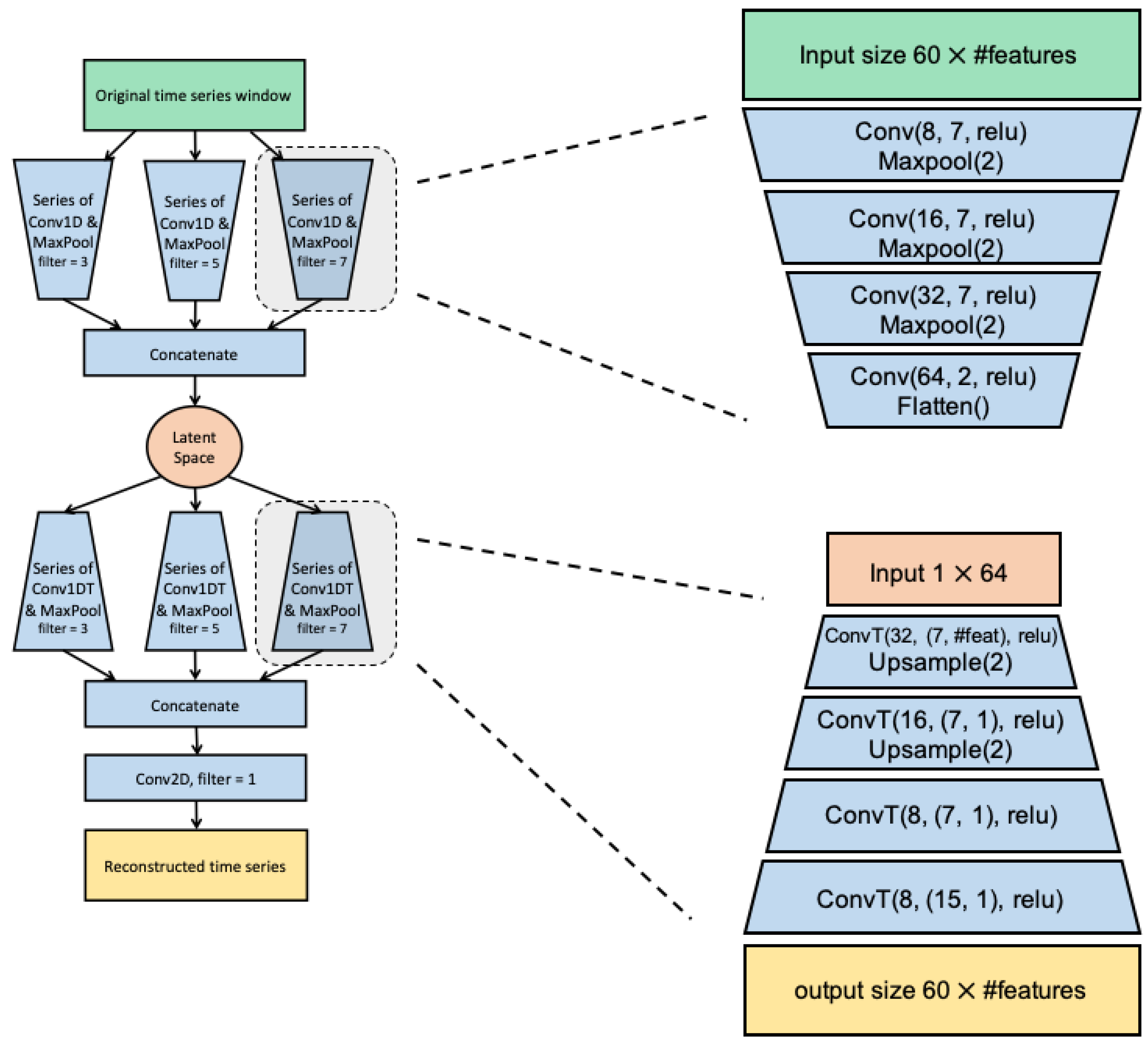
CVAE uses windowed time-series data as an input and applies series of convolutional operations with different filter sizes to take multiple local temporal dependencies into account. Then, the results of each series of convolutions are concatenated and mapped to the latent space. We use a similar architecture for both the encoder and the decoder. As a result, the decoder consists of a series of deconvolution and up-sampling with different filter sizes. Each branch of the encoder has four convolutional layers followed by a pooling layer, of which the number of input channels increases as the window size shrinks. Similarly, the decoder consists of four layers of de-convolution followed by an up-sampling layer, the number of input channels of which decreases as the window size expands. The exact number of layers depends on the size of the inputted time series windows, as we shrink the window size to 1 × # channels before the latent space layer. Figure 2 shows the general architecture used for all of the results presented in the paper. We treat the dimension of the latent space as well as β as hyperparameters that need tuning for each application, and we use the limited number of labels available to show what combinations performed best in a post-processing step.

3.4. Anomaly Detection Metric

Once CVAE is trained, we use the reconstruction errors obtained from the training data to set a threshold for detecting anomalies. To do so, we first calculate the reconstruction error for all training data, i.e., ζ i = | | x i x ^ i | | 2 2 , for i { 1 , , N train } , where x ^ i = D θ E ϕ x i (with D denoting the decoder and E the encoder). Once the reconstruction error is defined for the entire training dataset, we define the threshold for anomaly detection as
t h r = E [ ζ ] + 2 σ ( ζ )
where E and σ represent the expected value and the standard deviation. In the above equation, we set the threshold according to the prior knowledge that ∼2 % of the data are anomalous. As a result, we expect that the top 2 % tail of the reconstruction error corresponds to the anomalous examples, assuming that the reconstruction error follows a Gaussian distribution. If testing on a different data, the threshold formula needs to be adjusted according to the ratio of anomalous/nominal examples. Once the threshold is identified, we identify anomalies in the test data by calculating the reconstruction error for each test data instance and compare it to the above threshold. It should be noted that the model is fully unsupervised, and we only use test data to evaluate the performance of CVAE in a post-processing step.

4. Results and Discussion

Throughout this section, we compare performance of the proposed CVAE to five alternatives: (1) Conv-AE, which is a deep Auto-Encoder with convolutional architecture (identical to CVAE, except that it is not variational) and serves as a comparison to CVAE with small values of β , (2) FC-AE, which is a deep Auto-Encoder with fully connected architecture (architecture is reported in Appendix A), (3) BiGAN, which is anomaly detection based on deep Bidirectional GANs [26] (architecture is reported in Appendix A), (4) KMeans, which is a clustering-based anomaly detection, and (5) One-Class SVM (OC-SVM), which is an unsupervised kernel-based classification algorithm.
In any scenario, we divide the data into three sets of training, validation, and testing. We use training to train CVAE, validation to tune the hyper-parameters (i.e., dimension of latent space and β ) with limited available labels, and testing to evaluate the unbiased estimate of the model’s performance with a threshold (Equation (13)) calculated just based on the training set.

4.1. Validation on Yahoo!’s Data

We first comprehensively validate performance of CVAE on the recently published benchmark data set of Yahoo! for time series anomaly detection [39]. This dataset is comprised of four different time series: A1-4. A1 and A2 are univariate real and synthetic production traffic to some of the Yahoo! properties, respectively. A3 and A4 are synthetic multivariate time series with outlier and change-point anomalies, respectively. The multivariate data have additive noise and 12-h, daily, and weekly seasonality associated with the actual values of the traffic.
In all of the results, we assume that nominal data are the negative class, and the anomalous data are the positive class. We evaluate the performance of all models according to two metrics of precision and recall defined as
precision = T P T P + F P recall = T P T P + F N
where T P is true positive: anomalies that are correctly identified, F P is false positive (or false alarms): anomalies that are incorrectly identified, and F N is false negative, or anomalies that are missed and classified as nominal by mistake.
Figure 3 shows the precision (top panel) and recall (bottom panel) for the performance of classification on test data for each of the above-mentioned methods. Each data instance is a windowed time series, where, for A1 and A2, we use a window size of 50, and, for A3 and A4, we use a window size of 20 across all methods. We have also fixed the dimension of the latent space for CVAE, Conv-AE, FC-AE, and BiGAN to two dimensions for A1 and A2 and to 25 dimensions for A3 and A4. The value of hyperparameter β is fixed to 0.001 for these data sets. The reason for using a small value of hyperparameter β is that anomalies in Yahoo! data are point anomalies (anomalies that happen only in one time step) and, as a result, a lower value of β allows higher variance and complexity in the model, which leads to a better performance in the case of point anomalies. As mentioned above, for small values of β , the CVAE is similar to a Conv-AE, as can be seen from their performance across the data sets. For KMeans, we cluster the data into two clusters ( K = 2 ) and select the minority cluster to be representative of anomalies, and, for OC-SVM, we set the parameter ν = 10 % , which corresponds to the average expected percentage of anomalous examples present in the Yahoo!’s data and we used ’rbf’ kernel with coefficient set uniformly across features.
Across the four data sets, CVAE achieves 66.4 % precision and 68.4 % recall on average, which is very close to Conv-AE, especially in recall ( 75.5 % precision and 68.8 % recall). CVAE outperforms classic methods such as KMeans and OC-SVM, with an on-average 48.2 percentage point (pp) higher precision and 29.2 pp higher recall. Moreover, CVAE outperforms other deep learning-based anomaly detection approaches (FC-AE and BiGAN) on average by 43.8 pp (precision) and 60.2 pp (recall). As mentioned before, since the anomalies in the Yahoo! data are point anomalies, models with high variance such as Conv-AE and the CVAE with a small value of β perform better. In the next section, we showcase the performance of these methods on a different case study, where a model with higher bias performs better.

4.2. Anomaly Detection in FOQA Data

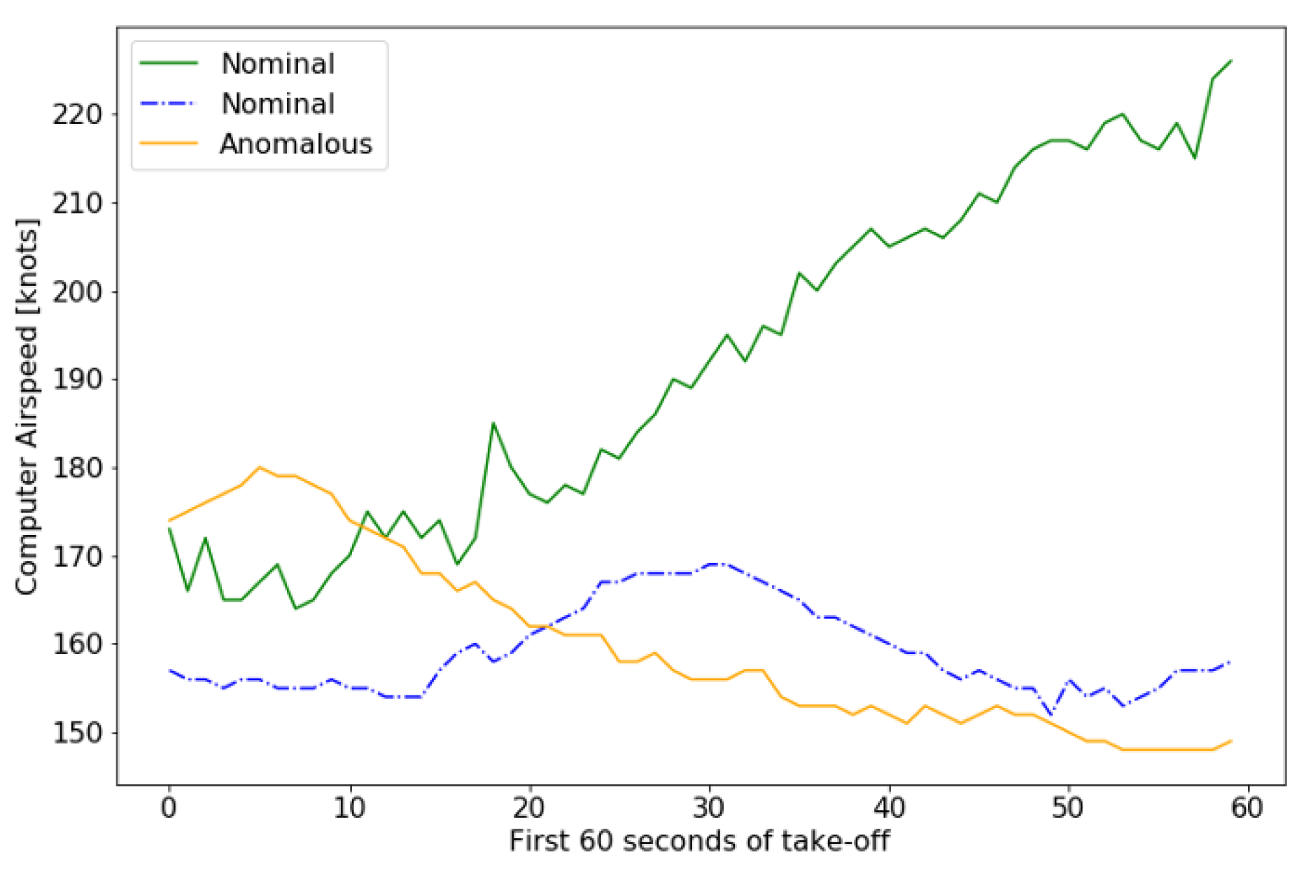
In this section, we introduce an anomaly detection case study based on FOQA data. In this case study, we are interested in identifying anomalies during take-offs of commercial flights, due to a drop in airspeed over a certain threshold. Subject matter experts have identified that, if the speed of an aircraft drops more than 20 knots in the first 60 s after take-off, an adverse event could ensue. To objectively measure the performance of the anomaly detection algorithm, we are relying on this specific safety incident. This is not necessarily the only type of anomaly in the data set and the true number of operationally significant safety anomalies are unknown; however, our objective is to measure the effectiveness of the algorithm and are using this particular safety incident as one measure of the algorithm’s performance. As a result, we have pre-processed FOQA data to set up training/validation/testing data sets for benchmarking machine learning models. Data consist of ∼27 K nominal and ∼700 anomalous samples. Each data sample is a multivariate time series of 16 features measuring the roll attitude, altitude information, pitch attitude, speed information, and yaw attitude. It should be noted that FOQA data contain hundreds of features, and the 16 features used in our study were selected due to their relevance to the take-off phase of flight based on the guidance of subject matter experts. Flights that experienced a drop in airspeed of more than 20 knots were given a label of 1; other flights were labeled as 0. Figure 4 visualizes three instances: both the green and blue lines represent nominal samples, while the orange line represents an anomalous sample. It can be seen that the pattern of a nominal example (e.g., blue line) can be very close and similar to an anomalous one (e.g., orange line).
Although data labels were used to differentiate nominal and anomalous flights, our intent is to assess whether a machine learning model can identify rarely occurring anomalous events in an unsupervised setting without prior knowledge of the significance or the characteristics of the event. The architecture of the CVAE (and Conv-AE) is deliberately based on the different groups of features outlined above. CVAE sends each group into its own encoder (as illustrated in Figure 2) and concatenates the outcome of each encoding before passing the information to the shared latent space. After that, each group has its own decoder to reconstruct the inputs by sampling from the shared latent space. This grouping is done purely based on domain expert knowledge of the flight dynamics of the aircraft and the corresponding observed variables, without any correlation analysis, so that learning proceeds in an unsupervised fashion. For all of the deep generative models (i.e., CVAE, Conv-AE, FC-AE, and BiGAN), we fix the dimensionality of the latent space to 10 dimensions. For KMeans, we cluster the data into two clusters ( K = 2 ) and select the minority cluster to be representative of anomalies, and, for OC-SVM, we set the parameter ν = 2.5 % , which corresponds to the expected percentage of anomalous examples present in the training data and we used ’rbf’ kernel with coefficient set uniformly across features. We also fix the hyperparameter β for CVAE to a larger value of 0.1 in this example. As we noted before, the anomalies in the FOQA data are not point anomalies and the entire data contained in a 60-s window (or a significant portion thereof) are needed to identify an anomalous example. As a result, we expect higher values of β to perform better, since they increase the amount of bias in the model, forcing the algorithm to not over-fit to anomalous training data. CVAE model is implemented in Python and using Keras library. Training of the CVAE (for 100 epochs) takes about 16.5 min and uses about 4.7 GB of memory on NASA’s Pleiades Supercomputer’s Skylake GPU-enhanced node (https://www.nas.nasa.gov/hecc/resources/pleiades.html) and testing on a single data point is in real-time.
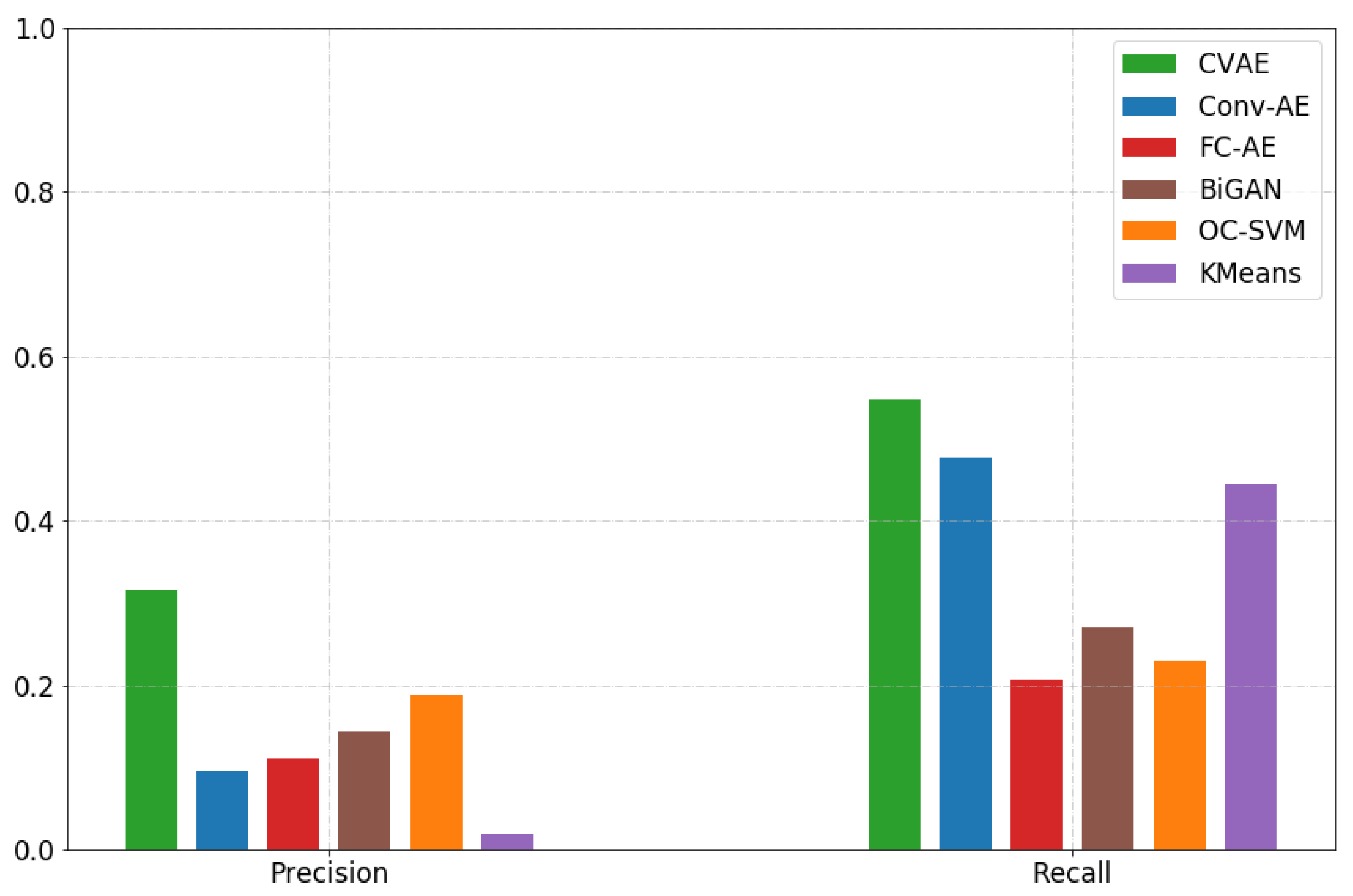
Figure 5 shows the performance of CVAE on this challenging case study, compared to the alternative methods. As is illustrated, CVAE outperforms all of the alternative methods both in precision and recall.
First, we want to emphasize the difference between CVAE and Conv-AE. As mentioned before, Conv-AE is similar to a CVAE with a small value of β , and, in the Yahoo! data, we saw that the performance of the two was very similar. However, in this case study, because anomalies happen over a window of data, we see that CVAE with β = 0.1 outperforms Conv-AE. The flexibility of balancing the bias/variance trade-off by tuning the hyperparameter β is the main advantage of using CVAE in place of regular autoencoders. On average, CVAE has a 23 pp higher precision and 7.2 pp higher recall compared to Conv-AE. Moreover, CVAE outperforms other deep learning-based approaches (e.g., BiGAN and FC-AE) with a 18.9 pp higher precision and 31 pp higher recall on average, and classic approaches (e.g., KMeans and OC-SVM) with a 21.3 pp higher precision and 21 pp higher recall.
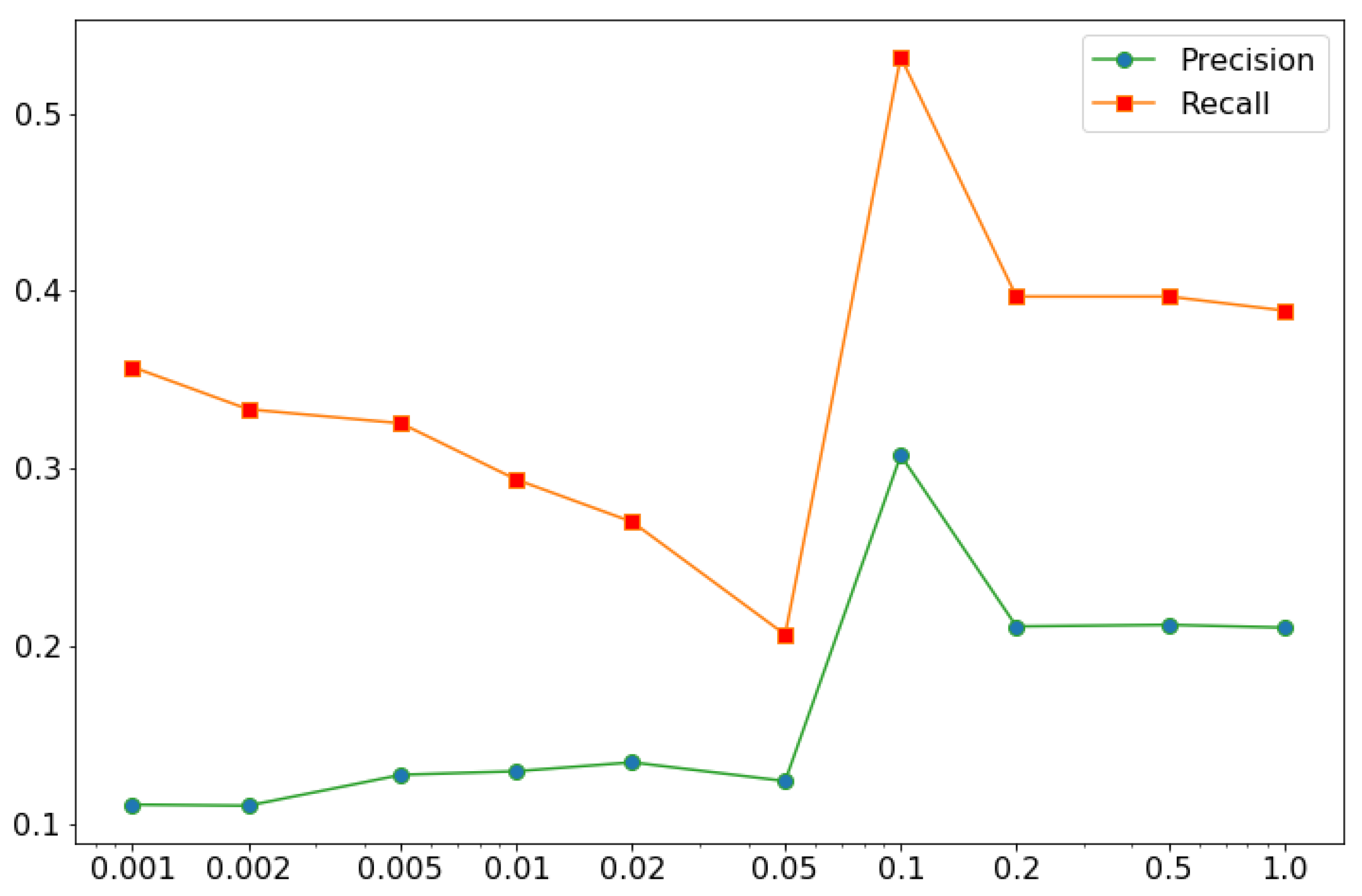
As mentioned above, we expect higher values of the hyperparameter β to perform better when dealing with anomaly detection examples where anomalies occur over the span of a time window. To further validate this conjecture, we illustrate CVAE’s performance in terms of precision and recall on the testing data on a wider range of values of hyperparameter β (Figure 6). Our intuition was partially correct, which illustrates an important finding. Although β = 0.1 performs better than smaller values, higher values of β do not improve performance. We conclude that β = 0.1 is a sweet spot for balancing the bias/variance trade-off of the model. This is significant because it emphasizes the importance of tuning hyperparameter β (which is the penalty imposed on the KL-divergence in the loss function in Equation (12)), depending on the data set and research question. As was illustrated in two examples (Yahoo! and FOQA data), depending on the domain and the nature of anomalies, a regular autoencoder, a variational autoencoder, or a model in-between the two, can demonstrate superior anomaly-detection performance. CVAE, as introduced in this study, allows flexibility in setting up the autoencoder model based on the problem at hand.
In many recent studies on anomaly detection using deep generative models [24,29,33,34], researchers rely on only training the models with nominal data (anomalies are not present during training and validation and only appear during testing), which can significantly improve model performance. To showcase this phenomenon, we trained CVAE on a training data set that only contains nominal examples and then test it on a testing data set of mixed nominal and anomalous examples. The ratio of anomalous to nominal samples in the testing data are still the same as before; the only difference is that we removed anomalous examples from the training and validation data sets. Figure 7 compares the performance of CVAE when trained with only nominal examples or mixed nominal/anomalous examples. In the case of mixed training data, we used the same setting as before ( β = 0.1 ), while in the case of only nominal training data, we decreased the value of hyperparameter β to 0.001 to achieve a closer fit to the training data. This is because we are aware that the training data do not contain any anomalies and CVAE can be allowed to closely fit to the nominal patterns in the training data. As expected, removing anomalies from the training data significantly improved CVAE’s performance, resulting in a 36.8 pp higher precision and 27.3 pp higher recall.
These results show a promising first step in developing and deploying an unsupervised and scalable machine learning algorithm based upon recent advancements in deep generative models—an algorithm that is able to identify anomalies in high-dimensional flight time series with reasonable accuracy and a minimal number of false negatives (i.e., missed anomalies).

5. Conclusions

In order to improve and automate identification of unknown vulnerabilities in flight operations, we have developed an unsupervised machine learning approach for identifying operationally significant anomalies in high-dimensional heterogeneous aviation time-series. The proposed approach constructs models based on observed operations and identifies operationally significant safety anomalies. This algorithm is demonstrated to have improved performance as compared to existing anomaly detection methods used in the aviation domain. This translates to increased visibility of previously undetected vulnerabilities that if gone unmonitored and unaddressed may lead to a more serious incident or accident. The majority of approaches presented in the aerospace literature either rely on rule-based thresholding or supervised learning approaches. Although the supervised approaches show a good performance, creating labels for aviation data requires a huge amount of effort and is largely impractical. Our approach builds upon recent advancements in deep generative models to develop the Convolutional Variational Auto-Encoder (CVAE), which is an unsupervised approach for anomaly detection in high-dimensional heterogeneous time-series data (Figure 1). It is important to note that there is a significant cost to missing each unknown incident and any improvement upon the detection rates helps to increase awareness and consequently safety. Having an unsupervised method that does not require valuable subject matter expert’s feedback can assist in this process and is a key aspect of being proactive to reduce incident and accident levels in anticipation of growing air traffic demands in the future.
We validate CVAE in relation to several classic approaches (e.g., KMeans clustering and one-class support vector machines) as well as deep learning-based approaches (e.g., autoencoder, generative adversarial networks), used in the literature for anomaly detection in various data sets. Validating CVAE on Yahoo!’s benchmark time series anomaly detection database, we show that our model outperforms both classic approaches (∼48 pp higher precision, and ∼29 pp higher recall) and deep learning based approaches (on average ∼44 pp higher precision and ∼60 pp higher recall) (Figure 3). Moreover, we illustrated the effect of hyperparameter β in the CVAE model on the performance of anomaly detection and illustrated the advantage of CVAE over autoencoders as well as conventional variational autoencoders (Figure 6).
The application of CVAE to anomaly detection in Flight Operational Quality Assurance (FOQA) shows promise for further development of this line of work for anomaly detection in high-dimensional heterogeneous time series. Specifically, by designing a case study of anomaly detection in the first 60 s of the take-off of commercial flights, we show that CVAE outperforms all baseline models (on average ∼20 pp higher precision and ∼26 pp higher recall) (Figure 5). Performance significantly improves when CVAE is only trained on nominal data as illustrated in Figure 7 (on average ∼37 pp higher precision and ∼27 pp higher recall).
Future Work: The next steps will potentially focus on developing an architecture to process different types of heterogeneous time series data, such as binary channels or categorical features in the FOQA data. One possible approach may be to map multiple inputs into a state space representation to capture the changes in the time series modes. In addition, exploring techniques to visualize and explain the behavior in the latent space as it relates to the original input parameters and the anomalies identified is another area of research that can add understanding and interpretability to the anomaly detection model. Finally, the scaling and practical deployment of the algorithm on more complex operationally significant real-world data sets would need to be tested and validated before the algorithm can be integrated into an existing vulnerability discovery program.

Author Contributions

All authors conceived the idea together. B.M. provided domain expertise and set up the F.O.Q.A. case study. M.M. developed the methodology and implementations of the method and performed validations and obtained the results. I.A. developed comprehensive literature review of anomaly detection in aerospace using machine learning. All authors contributed to the writing of the manuscript. All authors have read and agreed to the published version of the manuscript.

Funding

This research was supported by the NASA Airspace Operation and Safety Program and the NASA System-wide Safety Project.

Acknowledgments

The authors acknowledge the funding of this research from a NASA System-wide Safety Project under contracts 80ARC020D0010 and NNA16BD14C. We would also like to thank Hamed Valizadegan, Thomas Templin, Daniel Weckler, and Marc-Henri Bleu-Laine for their insights and comments in developing and testing the algorithm.

Conflicts of Interest

The authors declare no conflict of interest.

Abbreviations

The following abbreviations are used in this manuscript:
NASNational Airspace System
CVAEConvolutional Variational Auto-Encoder
FOQAFlight Operational Quality Assurance
NTSBNational Transportation Safety Board
FAAFederal Aviation Administration
ASIASAviation Safety Information and Sharing
IGInspector General
OC-SVMOnce-Class Support Vector Machine
BiGANBidirectional Generative Adversarial Networks
VIVariational Inference
MCMCMarkov Chain Monte Carlo
KLKullback–Leibler
FC-AEFully Connected Auto-Encoder
Conv-AEConvolutional Auto-Encoder

Appendix A

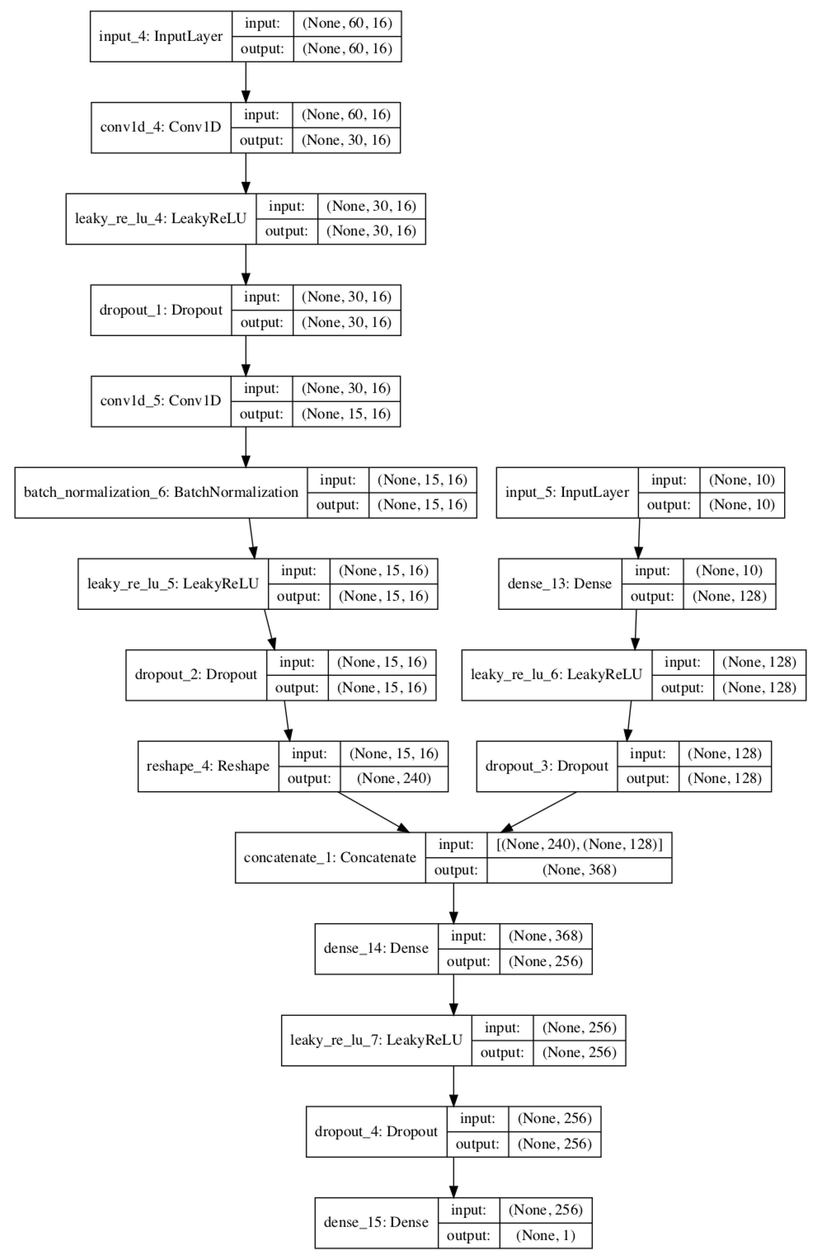
In this section, we report the architecture of the fully connected autoencoder (FC-AE) and the bidirectional generative adversarial network (BiGAN) for the interested reader. FC-AE encoder is comprised of a Time Distributed Dense layer with one neuron to mix different features of each windowed data instance, followed by three Dense layers with 100 neurons, followed by transition to the latent space (which is a Dense layer with the number of neurons equal to the dimension of the latent space). The decoder is similar and starts with three Dense layers with 100 neurons followed by a Time Distributed Dense layer with neurons equal to the number of features to reconstruct each feature. The BiGAN architecture is similar to that of [26]; the only differences are adjustments to the shapes and sizes of inputs and outputs and replacements of 2D convolutions by 1D convolutions, since the original model was developed for imagery data. Figure A1 shows the architecture of the discriminator as an example.
Figure A1. Network architecture of the discriminator in BiGAN.
Aerospace 07 00115 g0a1

References

  1. National Transportation Safety Board (NSTB). Annual Summaries of US Civil Aviation Accidents. 2019. Available online: https://www.ntsb.gov/investigations/data/Pages/aviation_stats.aspx (accessed on 8 August 2020).
  2. National Transportation Safety Board (NSTB). US Transportation Fatality Statistics. 2017. Available online: https://www.bts.gov/content/transportation-fatalities-mode (accessed on 8 August 2020).
  3. Sprung, M.J.; Chambers, M.; Smith-Pickel, S. Transportation Statistics Annual Report; U.S. Department of Transportation: Washington, DC, USA, 2018.
  4. FAA Office of Air Traffic Organization. Safety Management System Manual. 2019. Available online: https://www.faa.gov/air_traffic/publications/media/ATO-SMS-Manual.pdf (accessed on 8 August 2020).
  5. National Transportation Safety Board (NSTB). National Transportation Safety Board Aviation Investigation Manual Major Team Investigations. 2002. Available online: https://www.ntsb.gov/investigations/process/Documents/MajorInvestigationsManual.pdf (accessed on 8 August 2020).
  6. Office of Inspector General Audit Report. FAA’s Safety Data Analysis and Sharing System Shows Progress, but More Advanced Capabilities and Inspector. 2014. Available online: https://www.oig.dot.gov/sites/default/files/FAA%20ASIAS%20System%20Report%5E12-18-13.pdf (accessed on 8 August 2020).
  7. Office of Inspector General Audit Report. INFORMATION: Audit Announcement | FAA’s Implementation of the Aviation Safety Information Analysis and Sharing (ASIAS) System. 2019. Available online: https://www.oig.dot.gov/sites/default/files/Audit%20Announcement%20-%20FAA%20ASIAS.pdf (accessed on 8 August 2020).
  8. National Transportation Safety Board (NSTB) Assumptions Used in the Safety Assessment Process and the Effects of Multiple Alerts and Indications on Pilot Performance. Dist. Columbia Natl. Transp. Saf. Board. 2019. Available online: https://trid.trb.org/view/1658639 (accessed on 8 August 2020).
  9. Federal Aviation Administration. Flight Operational Quality Assurance. Technical Report; 2004. Available online: https://www.faa.gov/regulations_policies/advisory_circulars/index.cfm/go/document.information/documentID/23227 (accessed on 8 August 2020).
  10. Lee, H.; Madar, S.; Sairam, S.; Puranik, T.G.; Payan, A.P.; Kirby, M.; Pinon, O.J.; Mavris, D.N. Critical Parameter Identification for Safety Events in Commercial Aviation Using Machine Learning. Aerospace 2020, 7, 73. [Google Scholar] [CrossRef]
  11. Janakiraman, V.M. Explaining Aviation Safety Incidents Using Deep Temporal Multiple Instance Learning. In Proceedings of the 24th ACM SIGKDD International Conference on Knowledge Discovery and Data Mining (KDD ’18), London, UK, 19–23 August 2018; pp. 406–415. [Google Scholar]
  12. Bay, S.D.; Schwabacher, M. Mining distance-based outliers in near linear time with randomization and a simple pruning rule. In Proceedings of the Ninth ACM SIGKDD International Conference on Knowledge Discovery and Data Mining (KDD ’03), Washington, DC, USA, 24–27 August 2003; ACM: New York, NY, USA, 2003; pp. 29–38. [Google Scholar] [CrossRef] [Green Version]
  13. Budalakoti, S.; Srivastava, A.N.; Otey, M.E. Anomaly Detection and Diagnosis Algorithms for Discrete Symbol Sequences with Applications to Airline Safety. IEEE Trans. Syst. Man Cybern. Part C Appl. Rev. 2009, 39, 101–113. [Google Scholar] [CrossRef]
  14. Iverson, D.L. Inductive System Health Monitoring. In Proceedings of the International Conference on Artificial Intelligence, Las Vegas, NV, USA, 21–24 June 2004. [Google Scholar]
  15. Matthews, B.; Srivastava, A.N.; Schade, J.; Schleicher, D.; Chan, K.; Gutterud, R.; Kiniry, M. Discovery of Abnormal Flight Patterns in Flight Track Data. In Proceedings of the 2013 Aviation Technology, Integration, and Operations Conference, Los Angeles, CA, USA, 12–14 August 2013; p. 4386. [Google Scholar]
  16. Li, L.; Das, S.; Hansman, R.J.; Palacios, R.; Srivastava, A.N. Analysis of Flight Data Using Clustering Techniques for Detecting Abnormal Operations. J. Aerosp. Inf. Syst. 2015, 12, 587–598. [Google Scholar] [CrossRef] [Green Version]
  17. Das, S.; Matthews, B.; Srivastava, A.N.; Oza, N. Multiple Kernel Learning for Heterogeneous Anomaly Detection: Algorithm and Aviation Safety Case Study. In Proceedings of the 16th ACM SIGKDD International Conference on Knowledge Discovery and Data Mining, Washington, DC, USA, 24–28 July 2010; pp. 47–56. [Google Scholar]
  18. Hinton, G.; SAlakhutdinov, R. Reducing the Dimensionality of Data with Neural Networks. Science 2006, 313, 504–507. [Google Scholar] [CrossRef] [PubMed] [Green Version]
  19. Reddy, K.K.; Sarkar, S.; Venugopalan, V.; Giering, M. Anomaly Detection and Fault Disambiguation in Large Flight Data: A Multi-modal Deep Auto-encoder Approach. Annu. Conf. Progn. Health Monit. Soc. 2016, 7. Available online: http://www.phmsociety.org/node/2088/ (accessed on 8 August 2020).
  20. Guo, T.H.; Musgrave, J. Neural network based sensor validation for reusable rocket engines. In Proceedings of the 1995 American Control Conference-ACC’95, Seattle, WA, USA, 21–23 June 1995. [Google Scholar] [CrossRef]
  21. Zhou, C.; Paffenroth, R.C. Anomaly Detection with Robust Deep Autoencoders. In Proceedings of the 23rd ACM SIGKDD International Conference on Knowledge Discovery and Data Mining (KDD ’17), Halifax, NS, Canada, 13–17 August 2017; pp. 665–674. [Google Scholar]
  22. Kingma, D.P.; Welling, M. Auto-Encoding Variational Bayes. International Conference on Learning Representations (ICLR). 2013. Available online: https://arxiv.org/abs/1312.6114 (accessed on 8 August 2020).
  23. Rezende, D.J.; Mohamed, S.; Wierstra, D. Stochastic backpropagation and approximate inference in deep generative models. In Proceedings of the 31st International Conference on Machine Learning (ICML-14), Beijing, China, 21–26 June 2014; pp. 1278–1286. [Google Scholar]
  24. An, J.; Cho, S. Variational Autoencoder based Anomaly Detection using Reconstruction Probability. Spec. Lect. IE 2015, 2, 1–18. [Google Scholar]
  25. Xu, H.; Chen, W.; Zhao, N.; Li, Z.; Bu, J.; Li, Z.; Liu, Y.; Zhao, Y.; Peii, D.; Feng, Y.; et al. Unsupervised Anomaly Detection via Variational Auto-Encoder for Seasonal KPIs in Web Applications. In Proceedings of the 2018 World Wide Web Conference, Lyon, France, 23–27 April 2018; pp. 187–196. [Google Scholar]
  26. Zenati, H.; Foo, C.S.; Lecouat, B.; Manek, G.; Chandrasekhar, V.R. Adversarial feature learning. In Proceedings of the International Conference on Learning Representations, Toulon, France, 24–26 April 2017. [Google Scholar]
  27. Dumoulin, V.; Belghazi, I.; Poole, B.; Mastropietro, O.; Lamb, A.; Arjovsky, M.; Courville, A. Adversarially Learned Inference. In Proceedings of the International Conference on Learning Representations, Toulon, France, 24–26 April 2017. [Google Scholar]
  28. Donahue, J.; Krahenbuhl, P.; Darrell, T. Adversarially Learned Anomaly Detection. In Proceedings of the 20th IEEE International Conference on Data Mining (ICDM), Singapore, 17–20 November 2018. [Google Scholar]
  29. Chen, R.Q.; Shi, G.H.; Zhao, W.L.; Liang, C.H. Sequential VAE-LSTM for Anomaly Detection on Time Series. arXiv 2019, arXiv:1910.03818. [Google Scholar]
  30. Wang, X.; Du, Y.; Lin, S.; Cui, P.; Shen, Y.; Yang, Y. adVAE: A self-adversarial variational autoencoder with Gaussian anomaly prior knowledge for anomaly detection. Knowl. Based Syst. 2019, 190, 105187. [Google Scholar] [CrossRef] [Green Version]
  31. Zhang, C.; Chen, Y. Time Series Anomaly Detection with Variational Autoencoders. arXiv 2019, arXiv:1907.01702. [Google Scholar]
  32. Zhang, C.; Song, D.; Chen, Y.; Feng, X.; Lumerzanu, C.; Cheng, W.; Ni, J.; Zhang, B.; Chen, H.; Chawla, N.V. A Deep Neural Network for Unsupervised Anomaly Detection and Diagnosis in Multivariate Time Series Data. In Proceedings of the AAAI-19, Honolulu, HI, USA, 27 January–1 February 2019; pp. 1409–1416. [Google Scholar]
  33. Park, D.; Hoshi, Y.; Kemp, C.C. A Multimodal Anomaly Detector for Robot-Assisted Feeding Using an LSTM-Based Variational Autoencoder. IEEE Robot. Autom. Lett. 2018, 3, 1544–1551. [Google Scholar] [CrossRef] [Green Version]
  34. Su, Y.; Zhao, Y.; Niu, C.; Liu, R.; Sun, W.; Pei, D. Robust Anomaly Detection for Multivariate Time Series through Stochastic Recurrent Neural Network. In Proceedings of the 25th ACM SIGKDD International Conference on Knowledge Discovery and Data Mining (KDD ’19), Anchorage, AK, USA, 4–8 August 2019; pp. 2828–2837. [Google Scholar]
  35. Higgins, I.; Matthey, L.; Pal, A.; Burgess, C.; Glorot, X.; Botvinick, M.; Mohamed, S.; Lerchner, A. β-VAE: Learning Basic Visual Concepts With A Constrained Variational Framework. In Proceedings of the International Conference on Learning Representations (ICLR), Toulon, France, 24–26 April 2017. [Google Scholar]
  36. Doersch, C. Tutorial on Variational Autoencoders. arXiv 2016, arXiv:1606.05908. [Google Scholar]
  37. Chen, T.Q.; Li, X.; Grosse, R.B.; Duvenaud, D.K. Isolating Sources of Disentanglement in Variational Autoencoders. Adv. Neural Inf. Process. Syst. (NeurIPS) 2018, 31, 2610–2620. [Google Scholar]
  38. Kim, H.; Mnih, A. Disentangling by Factorising. In Proceedings of the International Conference on Machine Learning (ICML), Vancouver, BC, Canada, 30 April –3 May 2018. [Google Scholar]
  39. Yahoo!-Webscope. Dataset Ydata-Labeled-Time-Series-Anomalies-v10. 2019. Available online: https://webscope.sandbox.yahoo.com/catalog.php?datatype=s&did=70 (accessed on 8 October 2019).
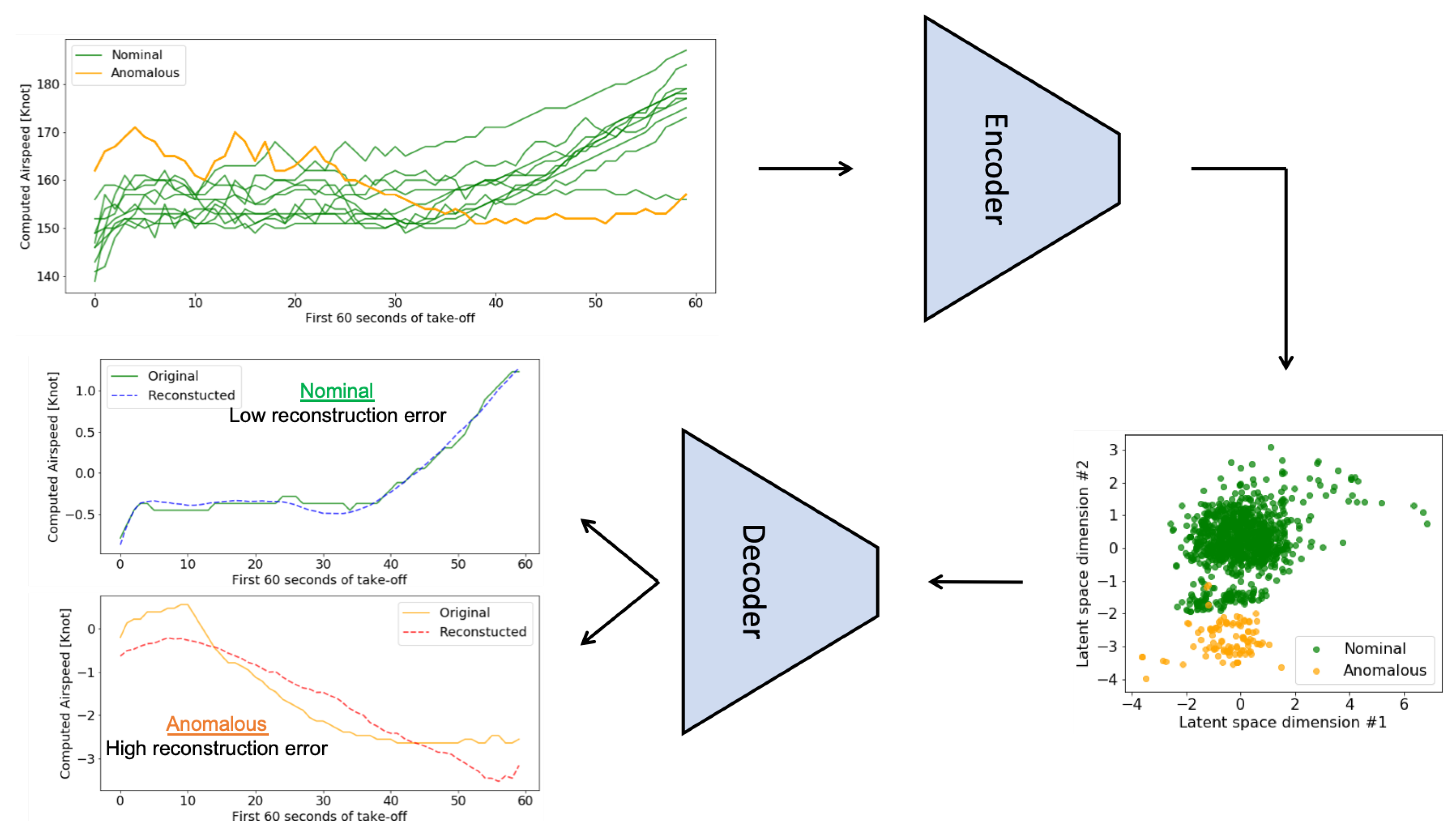
Figure 1. Overview of the proposed unsupervised anomaly detection approach.
Aerospace 07 00115 g001
Figure 2. Network architecture of the Convolutional Variational Auto-Encoder (CVAE). On the right panels, (i) Conv depicts 1D convolution, where the first input is the channel (or filter) size, the second is the kernel size, and the third is the activation function, (ii) Maxpool refers to max pooling operation, (iii) ConvT refers to 2D transpose convolution with the first input is channel (or filter) size, the second input is kernel size, and the third is the activation function, and (iv) Upsample refers to the up sampling. It should be noted that only the first layer of the decoder performs 2D transpose convolution to build the feature dimension and the remaining layers do not expand the feature dimension.
Aerospace 07 00115 g002
Figure 3. Anomaly detection in Yahoo!’s data using KMeans, OC-SVM, FC-AE, Conv-AE, CVAE, and BiGAN. It should be noted that FC-AE and BiGAN performances are absolute zero in the case of A2 data, since they both detect all of data in the testing set as nominal.
Aerospace 07 00115 g003
Figure 4. Computer airspeed during the first 60 s of take-off for three samples.
Aerospace 07 00115 g004
Figure 5. Validating the performance of CVAE on the FOQA data against Conv-AE, FC-AE, BiGAN, OC-SVM, and KMeans.
Aerospace 07 00115 g005
Figure 6. CVAE’s performance on the FOQA case study with different values of hyperparameter β .
Aerospace 07 00115 g006
Figure 7. CVAE’s performance when trained only on nominal data or a mixture of nominal/anomalous data.
Aerospace 07 00115 g007