Computational Evaluation of Control Surfaces Aerodynamics for a Mid-Range Commercial Aircraft

Abstract

Computational fluid dynamics is employed to predict the aerodynamic properties of the prototypical trailing-edge control surfaces for a small, regional transport, commercial aircraft. The virtual experiments are performed at operational flight conditions, by resolving the mean turbulent flow field around a realistic model of the whole aircraft. The Reynolds-averaged Navier–Stokes approach is used, where the governing equations are solved with a finite volume-based numerical method. The effectiveness of the flight control system, during a hypothetical conceptual pre-design phase, is studied by conducting simulations at different angles of deflection, and examining the variation of the aerodynamic loading coefficients. The proposed computational modeling approach is verified to have good practical potential, also compared with reference industrial data provided by the Leonardo Aircraft Company.

1. Introduction

Present trends in commercial aircraft design methodologies, which are mainly oriented toward cost reduction for product development, demand the accurate prediction of the control surfaces aerodynamics, to examine the aircraft flight control system early in the design process. The initial determination of handling qualities and hinge moments induced by the deflections of the different control surfaces permits significant improvements in the aircraft sizing process, with a strong impact on the aircraft weight prediction.

The computational approach is particularly useful in the pre-design process of a new aircraft, where wind-tunnel models are expensive and limited to the preselected parameters. The low-fidelity Vortex Lattice Method (VLM) is still widely used in evaluating the aerodynamic performance of the aircraft in the early design stages [1,2]. Owing to their high computational speed, VLM solvers give an immediate feedback on design changes, making quantitative knowledge available earlier in the design process. When considering a mid-range commercial aircraft, for example, a VLM approach was recently employed in the conceptual design for a regional turboprop aircraft in [3]. On the other hand, recent developments in meshing technology, numerical algorithms and calculation performance have allowed high-fidelity Computational Fluid Dynamics (CFD) models to be intensively used by industrial researchers to produce relevant aerodynamic databases. In fact, CFD has been strongly emerging as an effective tool for industrial aerodynamics research [4,5,6]. However, the application of CFD methods to simulate flight maneuvers is still a challenging task. The complex aerodynamic effects arising from the deflection of the different control surfaces, along with the consequent impact on the overall aircraft aerodynamics, and the importance of the flight envelope to be covered, make the numerical simulations particularly demanding. Therefore, while CFD has been usually employed to study the aerodynamics of high-lift systems during take-off and landing [7], the application to other control surfaces has been quite limited [8,9].

In this work, the aerodynamic analysis of the complete configuration of a regional transport aircraft is performed with a detailed assessment of the local aerodynamics of the trailing-edge control surfaces. The simulations are aimed at determining the variation of the aerodynamic loads, depending on the deflections of the control surfaces, and thus examining the effectiveness of the flight control process. Specifically, the efficiency of prototypical ailerons and elevators is studied, at typical flight conditions, by means of several different calculations. The mean turbulent flow field around the whole aircraft is simulated by using a fully three-dimensional CFD code employing the Finite Volume (FV) discretization approach, supplied with a Reynolds-Averaged Navier–Stokes (RANS) turbulence modeling procedure, e.g., [10,11]. Eddy viscosity-based diffusion is introduced into the governing equations to mimic the effects of turbulence, while solving an additional evolution equation for the turbulent viscosity variable. A similar approach was successfully adopted in other works investigating the aerodynamics of innovative regional aircraft models, e.g. [12,13]. The numerical simulations are conducted using the CFD software ANSYS Fluent 19, which is commonly and successfully employed for building virtual wind tunnels in industrial aerodynamics research [7,14,15,16].

The present analysis focuses on the validation of the proposed computational modeling approach with the distinctive feature of using real-case geometries, as provided by the Leonardo Aircraft Company researchers, rather than simplified generic wing-body models, as is typically done [7,17,18]. In fact, the main aim of this work is to examine the performance of CFD models that make use of relatively coarse FV meshes, to be employed for the conceptual design of a new mid-range commercial aircraft. A simplified CFD approach is evaluated, where the boundary layer region is not resolved [19], but modeled through a classical wall-function approach [20]. The numerical results are validated by comparison with wind-tunnel data obtained for similar models, and reference empirical data provided by the industrial aerodynamicists.

The remainder of this manuscript is organized as follows. In Section 2, the overall computational modeling approach is introduced, including the different geometric models that are employed in this study. The details of the CFD model implementation are given in Section 3. The results of the numerical simulations based on the present pre-design models are presented and discussed in Section 4. Finally, some concluding remarks are drawn in Section 5.

2. Computational Modeling

In this section, the overall computational modeling and simulation approach is introduced. The present analysis is performed using both low-fidelity and high-fidelity computational methods, as is typical during the preliminary design process to make a meaningful comparison. After briefly discussing the main features of the two different approaches, the geometric models that are used for the present simulations, involving both clean configuration and flight control surfaces, are illustrated.

2.1. Methodology

The prediction of the aerodynamic properties of interest is initially obtained using low-fidelity methods, by employing a VLM solver [1], while additional reference data are obtained using classical semi-empirical methods [21]. VLM uses singularities placed on the wing surface, while assuming an inviscid and incompressible flow field, which can be corrected using the Prandtl–Glauert compressibility correction. VLM solvers are ideally suited for the preliminary design environment, where they can be used to predict aerodynamic loads, stability and control data. Some aerodynamic characteristics as lift curve slope, lift distribution, and induced drag, can be obtained by modeling the wing through horseshoe vortices that are distributed along both span and chord, while neglecting the effects of thickness and air viscosity. In this study, a VLM-based free program for the aerodynamic and flight-dynamic analysis of a rigid aircraft of arbitrary configuration is used [22]. In this framework, wings are created as lifting surfaces, while the fuselage is considered to be a slender body. Suitable input data files must be created for describing the aircraft model under study. In particular, for each lifting surface, the geometry of the different wing sections must be provided, along with reference values for calculating the main aerodynamic coefficients and the appropriate vortex density parameter. The actual VLM model that is employed in this study is presented in Section 4.2.1.

The aerodynamics of the flight control surfaces is more accurately predicted by using a high-fidelity method, namely by resolving the RANS governing equations, which describe the mean turbulent flow field around the aircraft. Following this approach, the whole range of turbulent flow scales is modeled through suitable closure models. The RANS governing equations, which are not reported here for brevity, can be found, for instance, in Wilcox [23]. RANS methods are commonly used for the numerical simulation of both compressible and incompressible aerodynamic flows, e.g., [11,24]. In this work, the standard version of the one-equation Spalart–Allmaras (SA) model is employed, as is implemented in the commercial CFD solver that is selected. According to this model, the effect of turbulence is approximated by means of eddy viscosity terms, where an additional evolution equation for a modified eddy viscosity variable is resolved along with the RANS governing equations [10]. Given the nature of the present study, for the sake of effectiveness, the turbulent boundary layer is modeled using a standard wall-function approach, where semi-empirical correlations are employed instead of resolving the near-wall region [19]. This way, the wall boundary conditions are implemented so that relatively coarse FV meshes can be used in the numerical simulations. In fact, the restriction of placing the first off-wall grid point in the viscous sub-layer, such that $y^{+}\approx 1$, would lead to an increase in the computational cost that is out of the scope of this preliminary design study, while the wall-modeling is a viable alternative that allows use of even $y^{+}\approx 60$, for the present calculations. However, the standard wall-function method, as is usually employed, has limitations for flow cases that involve high adverse pressure gradients and compressibility. The examination of more sophisticated wall-function approaches for the SA turbulence model, which were recently developed, e.g., [25], is deferred to future research.

2.2. Geometric Models

The present study focuses on the computational evaluation of the aerodynamics of the trailing-edge control surfaces of a mid-range commercial aircraft. Starting from the Computer-Aided Design (CAD) model of the complete aircraft provided by the Leonardo Aircraft Company, the present geometric models are slightly simplified to make the computational cost of the numerical simulations affordable in a typical pre-design phase. In particular, the effects of the propellers are not considered. However, to achieve a meaningful comparison with reference industrial data, the main features of the original models are maintained. The aerodynamic flow is described in a Cartesian coordinate system ($x, y, z$), where the three directions correspond to the roll, pitch, and yaw axes of the aircraft, respectively. The different geometrical models that are employed in the simulations are introduced in the following, both in clean configuration and with deployed control surfaces.

2.2.1. Clean Configuration

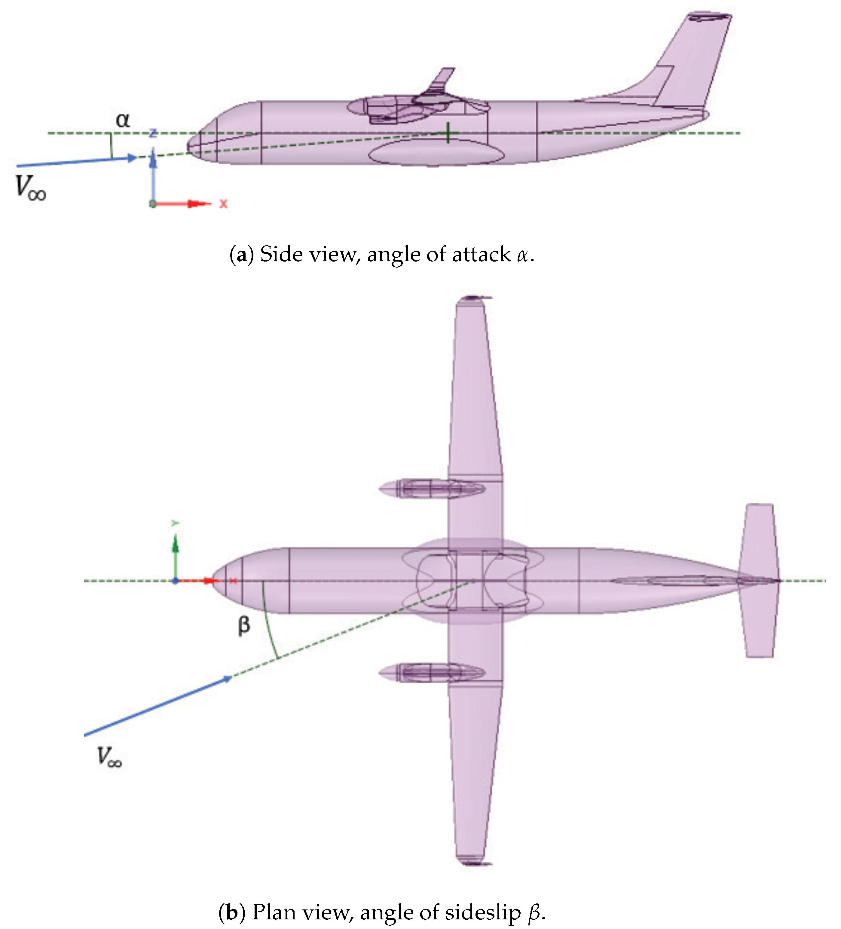
The geometric model that is used for the CFD calculations is illustrated in Figure 1, where the side and plan views of the regional transport aircraft under examination are depicted [13]. In this figure, $V_{\infty }$ represents the relative wind velocity, while $\alpha$ and $\beta$ stand for the Angle of Attack (AoA) and sideslip, respectively. The geometric model is comprised of fuselage, wing, empennage, and nacelle groups. Please note that the orientation of the reference body axes is such that the x-axis points backward, the y-axis points to the right wing, and the z-axis points upward. Some important geometrical data of the aircraft wing and tailplanes are given in

Table 1. Clean wings: geometrical data.

Parameter	Value
Wing Area	A
Wingspan (without winglets)	b
Wingspan (with winglets)	$1.03$b
Mean Aerodynamic Chord, $\overline{c}$	$0.086$b
Taper Ratio, $\lambda$	$0.5$
Horizontal Tailplane Area	$0.20$A
Horizontal Tailplane Span	$0.28$b
Vertical Tailplane Area	$0.25$A
Vertical Tailplane Span	$0.16$b

. Here, the different geometrical parameters are expressed in non-dimensional form, by using the wing area A and the wingspan b for normalization. The taper ratio $\lambda$ is defined as the ratio between the tip chord and the root chord of the wing. Note that some reference values cannot be reported, because they are not classified for publication by the industrial partner. However, the reference planform wing surface A is in the range from 70 to 80 m${}^2$, depending on the selected aircraft model in a family concept.

The model for the entire aircraft in clean configuration is obtained by not considering the gaps between the main aircraft components and the stowed control surfaces, while the projections of the surface edges are maintained, so that the different contributions of the different elements can be easily evaluated. The frontal view of the aircraft model is presented in Figure 2, where half the computational domain is considered, along with the associated surface mesh. Starting from the above model, the sub-model for analyzing the aerodynamics of the isolated clean wing is properly created by removing nacelles and winglets. This reduced model is employed for inviscid calculations that are preliminarily conducted to test the tool originally developed to evaluate the spanwise loading distribution starting from the CFD data. This way, the proper comparison with VLM results can be made.

2.2.2. Flight Control System

In this study, the flight control system is comprised of the main trailing-edge control surfaces that are the ailerons and the elevators. The different geometric models for evaluating the aerodynamics of these movable systems are developed by endowing the initial model of the aircraft provided by industrial aerodynamicists. Some geometrical data associated with the aircraft control surfaces are given in

Table 2. Clean surfaces: geometrical data.

Parameter	Value
Aileron Starting Section, $y_{start}^{\mathrm{aileron}}$	$\pm 0.725$$\frac{b}{2}$
Aileron Ending Section, $y_{end}^{\mathrm{aileron}}$	$\pm 0.992$$\frac{b}{2}$
Aileron Chord Ratio $c_a/c$	$0.3$
Elevator Starting Section, $y_{start}^{\mathrm{elevator}}$	$\pm 0.010$$\frac{b}{2}$
Elevator Ending Section, $y_{end}^{\mathrm{elevator}}$	$\pm 0.277$$\frac{b}{2}$
Elevator Chord Ratio, $c_e/c$	$0.33$
Horizontal Tailplane Incidence	$i_h<0$
Longitudinal Moment Arm	$z_h-z_w$
Tail-Wing Distance	$l_h$
Moment Reference Point	$0.25$$\overline{c}$

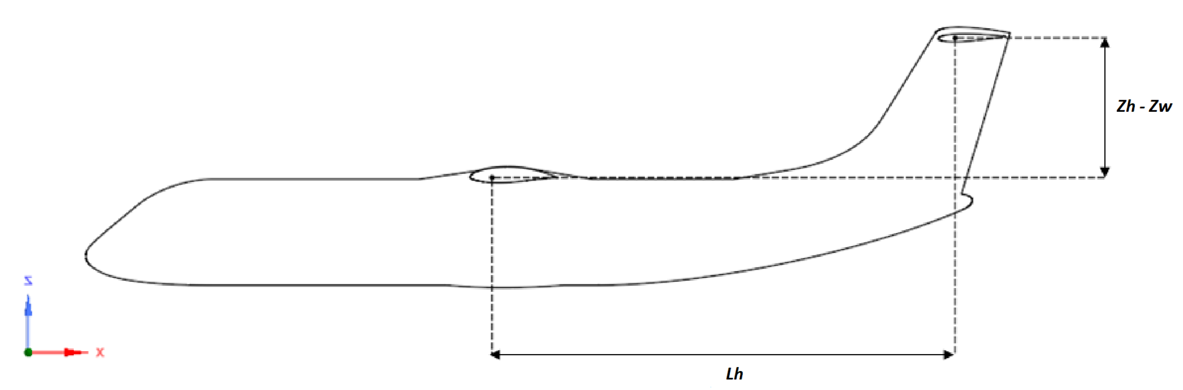
, with related definitions being illustrated in Figure 3. The characteristic high-wing T-tail empennage configuration of the regional transport aircraft under study is illustrated in Figure 4, where $z_h-z_w$ and $l_h$ represent the longitudinal moment arm and the vertical distance between the horizontal tailplane and the aircraft wing, respectively. The incidence of the horizontal tailplane is represented by $i_h$, which is the negative setting angle of the tailplane chord $c_h$ with respect to the $x-$axis direction.

The computational evaluation is performed by deflecting the control surfaces one at a time, while leaving the others in the stowed position. As far as the gaps between the moving surfaces and the correspondent main components are concerned, both upper and lower gaps are closed, whereas the lateral gaps are maintained, to avoid mesh distortion for deflected configurations. This way, the issue of meshing the main gaps, which represents a crucial part of the meshing process [26], is practically not addressed in this work.

The CAD model that is developed to study the aerodynamic effect of the ailerons is presented in Figure 5, along with the associated surface mesh, for the whole aircraft. The geometry is corresponding to that one considered for the clean configuration, while imposing two opposite deflection angles for the two ailerons, which are ${\delta }_a=\pm {10}^{\circ }$, with the right aileron being deflected downward. The corresponding close-up view is reported in Figure 6, along with the illustration of the positive deflection angle. The CAD model for studying the aerodynamic effect of the elevators is fully consistent with the approach used above. The computational grids are approximately corresponding to the previous ones, in terms of both number of elements and wall region resolution. For example, the side view of the rear part of the aircraft model with elevators deflected is illustrated in Figure 7, along with the associated surface mesh, for a given deflection angle that is ${\delta }_e=+{10}^{\circ }$ (downward).

3. CFD Solver Configuration

Some important settings about the CFD model implementation are made known in the following. The RANS governing equations are solved in a regular hexahedral domain, containing the aircraft models described above, whose size is chosen also based on a previous study conducted for a similar aircraft model [13]. The extents of the computational domain are provided in Figure 8, where both frontal and side views of half the model are shown. Please note that this computational domain is employed for all the flow configurations under study.

The numerical simulations presented in this work are carried out for zero sideslip angle ($\beta =0^{\circ }$). Therefore, the baseline calculations for the clean configuration, as well as the calculations performed to evaluate the effect of elevators, due to the symmetric flow configurations, make use of half the computational domain, while proper symmetry boundary conditions are imposed at the mid-span plane ($y=0$). On the contrary, the calculations for the aircraft with deflected ailerons, due to the asymmetric flow configuration, do employ the entire computational domain. In this case, the FV mesh generation is simplified by separately considering the two specular sub-domains, while putting a suitable mesh interface between them.

Hybrid meshes with tetrahedral elements and inflation layer in the wall region are employed for all the CFD calculations, with the mesh resolution representing a fair compromise between numerical accuracy and computational cost. Twelve prism layers, with a growth rate of $1.1$, are used in the boundary layer. Owing to the wall-function approach, a suitable first layer thickness is chosen, which allows proper modeling of the wall region. The FV meshes for the different flow configurations are developed by suitably modifying the baseline mesh used for the clean configuration. The latter, which is made up of about 7 million elements, was determined through a proper mesh sensitivity analysis, resulting in being the fair compromise between computational cost and estimation accuracy. Specifically, three different levels of resolution were tested by examining the deviation of the aerodynamic force coefficients. The deviation found between the finer and the medium mesh was considered small enough to state that a finer mesh would have not provided much more accurate results, but only increased the computational cost. For the selected FV grid, the mesh quality results in being pretty good, especially considering the complexity of the geometrical models. In fact, the maximum skewness of the mesh is less than $0.91$, which is within the prescribed limits for the commercial CFD code that is used. The same occurs for other mesh quality parameters, such as the aspect ratio and the orthogonal quality. For example, the plan view of the volume mesh for the configuration with deflected ailerons, corresponding to the half-span section of the right aileron, is shown in Figure 9. The use of the inflation layers in the wall region is apparent. It is worth stressing that given the aim of this work, which examines the feasibility and reliability of the proposed method during a hypothetical pre-design phase, the computations are performed using numerical meshes that are much coarser than those used in other similar numerical studies, e.g., [12], where more sophisticated turbulence models were employed.

The preliminary validation of the above CFD model is performed by considering a simplified wing-fuselage system, which is comprised of a round fuselage and a rectangular wing, where the NACA 0012 airfoil is used as symmetrical wing section. The model corresponds to one of the experimental combinations analyzed in the NACA Technical Report 540 [27]. Here, the aerodynamic interference between wing and fuselage, in the high-wing configuration, is examined at various angles of incidence, in symmetric flow. By making a comparison with the wind-tunnel data, the present CFD results are fully acceptable for small values of the AoA parameter, say $-5^{\circ }<\alpha <5^{\circ }$, as is illustrated in Figure 10, where the main aerodynamic coefficients are reported.

In this study, two different flight conditions are considered for the CFD simulations, namely a low speed condition that is typical of take-off and approach, with extended flaps, at $M_{\infty }=0.2$, and a normal cruise condition, at $M_{\infty }=0.52$. In the first, incompressible case, the energy equation is not solved, while imposing velocity inlet and pressure outlet boundary conditions. In the second, compressible case, the energy equation is solved supplied with the ideal gas law, while imposing pressure far field boundary conditions. The ratio of turbulent eddy viscosity to molecular viscosity is set to $0.1$ in the freestream. The AoA parameter is controlled by imposing the freestream velocity components. Please note that the solutions illustrated in the following figures are calculated at zero AoA, unless differently specified. The pressure-based coupled solver with second-order discretization is used for the numerical integration of the RANS equations. As for the computational time, typically, a calculation took about eight (twelve) hours, for the incompressible (compressible) case, using a parallel workstation that employed 16 Intel Xeon 2.4 GHz processors, for a minimum convergence threshold of ${10}^{-5}$.

4. Results

To demonstrate the capabilities of the proposed computational modeling framework in a real case, several CFD calculations are conducted using the geometric models introduced in Section 2.2. Specifically, RANS simulations of the mean turbulent flow field around the whole aircraft, with the control surfaces in either stowed or deployed positions, are carried out. The three different flow configurations presented in the following are summarized in

Table 3. Flow configurations.

Case	${\mathit{\delta }}_{\mathit{a}}$	${\mathit{\delta }}_{\mathit{e}}$
Clean Configuration	$0^{\circ }$	$0^{\circ }$
Ailerons Deflected	$\pm {10}^{\circ }$	$0^{\circ }$
Elevators Deflected	$0^{\circ }$	$\pm {10}^{\circ }$

.

The aerodynamic loading is expressed in terms of drag and lift coefficients that are $C_D=D/\left(q_{\infty }A\right)$ and $C_L=L/\left(q_{\infty }A\right)$, where D and L are the components of the mean aerodynamic force acting along and perpendicular to the relative wind direction, respectively, while $q_{\infty }=\frac{1}{2}{\rho }_{\infty }{V}_{\infty }^2$ stands for the dynamic pressure, with ${\rho }_{\infty }$ being the freestream air density. The three different moment coefficients are defined as $C_r$ (rolling), $C_m$ (pitching), and $C_n$ (yawing). Given the body axes reference depicted in Figure 1, it holds $C_r=-C_{M_x}$, $C_m=C_{M_y}$, and $C_n=-C_{M_z}$, with $M_x$, $M_y$, and $M_z$ being the moment components along the three spatial directions, where $C_{M_x}=M_x/\left(q_{\infty }A\overline{c}\right)$, and analogously for the other two directions. Practically, it is assumed $C_r>0$ when the rolling tends to put the right wing down, $C_m>0$ when the pitching tends to put the aircraft nose up, and $C_n>0$ when the yawing tends to put the aircraft nose right. The reference point for the moment evaluation is generally set coincident with the point at one quarter of the mean aerodynamic chord.

4.1. Clean Configuration

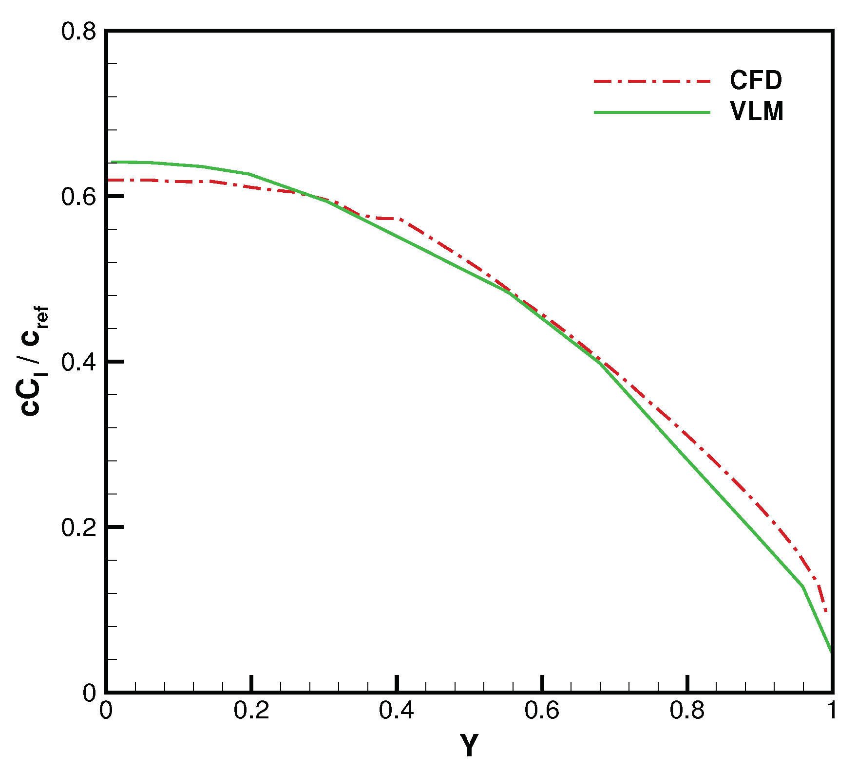
For the clean configuration, the solution obtained for the isolated wing model is first considered. The flight condition of the numerical test corresponds to a lift coefficient of $C_L=0.48$, at Mach number $M_{\infty }=0.2$. The inviscid CFD solution is compared to the VLM-based solution by examining the loading distribution along the spanwise direction. This calculation was conducted by neglecting the effect of both fluid viscosity and turbulent eddy viscosity, in order to verify the in-house tool that was originally developed to evaluate the spanwise loading distribution, starting from the available CFD data. The aerodynamic load is expressed in terms of the product $c{C}_l$, where c and $C_l$ stand for the local chord length and the section lift coefficient, respectively. The data are obtained using the strip method, by developing a suitable custom field function, where the aircraft wing is divided into several strips on which normal and tangential stresses are integrated. As demonstrated in Figure 11, where the chord length is normalized by the mean aerodynamic chord ($c_{ref}=\overline{c}$), and the abscissa $Y=y/(b/2)$ represents the normalized coordinate along the spanwise direction, the agreement between the two different solutions is fully acceptable.

The model of the complete aircraft in clean configuration is employed for several tests, whose results are also exploited as reference data for the solutions with deflected control surfaces. Several steady simulations are conducted at the two different flight conditions mentioned above, which can be expressed in terms of Mach and Reynolds numbers. The first one corresponds to $M_{\infty }=0.2$ and $R{e}_{\infty }=11.8\times {10}^6$, while the second one corresponds to $M_{\infty }=0.52$ and $R{e}_{\infty }=14.5\times {10}^6$. The aerodynamic loading coefficients are evaluated by integrating the predicted stresses on the aircraft surface. For illustration, the surface contours of the pressure coefficient, $C_p=(p-p_{\infty })/q_{\infty }$, and the skin friction coefficient, $C_f={\tau }_w/q_{\infty }$, are shown in Figure 12 and Figure 13, respectively, by considering both upper and lower plan views of the aircraft.

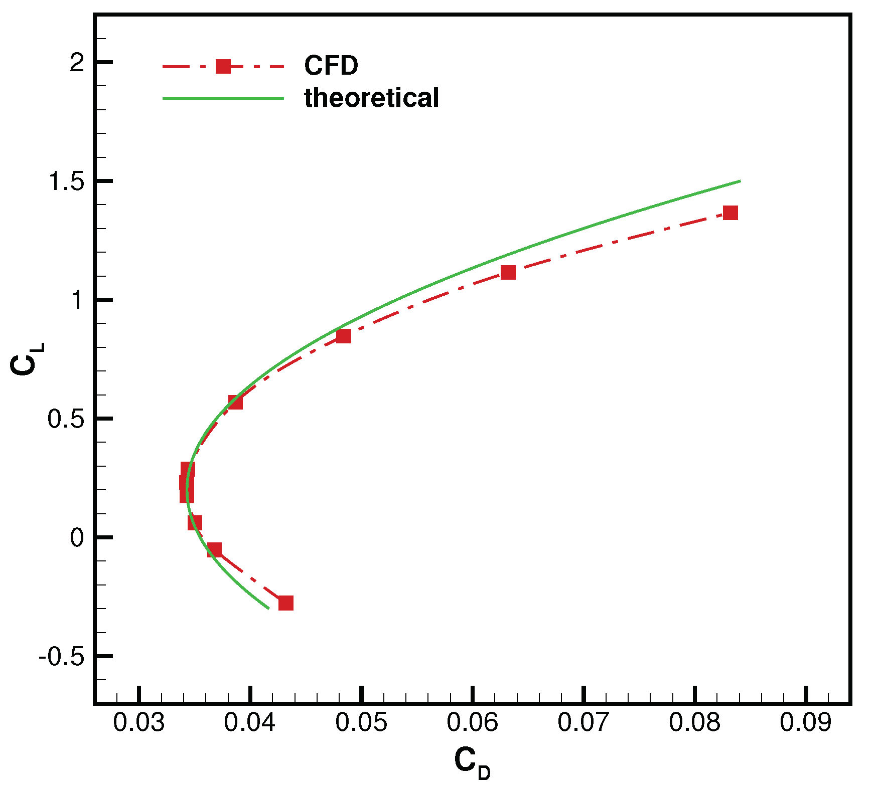
The drag polar, which is obtained by varying the AoA, is illustrated in Figure 14, compared with the theoretical parabolic polar, that is

$$C_D=C_{D0}+\frac{1}{e\pi AR}{(C_L-C_L^{\prime })}^2,$$

(1)

where $C_{D0}$ stands for the minimum drag coefficient, $AR$ is the aspect ratio, and e is the Oswald factor. Present CFD calculations provide $C_{D0}$ equal to $0.034$ or, equivalently, 340 drag counts, which corresponds to $C_L^{\prime }\approx 0.2$ for the lift coefficient. By exploiting the parabolic curve fitting the present numerical data, the value of $0.9$ is estimated for the Oswald factor. Apparently, the lift coefficient is well predicted for a reasonable operative range of the AoA parameter.

The variation of the pitching moment coefficient $C_m$ against the AoA is reported on the left side of Figure 15, corresponding to two different choices of the reference point for the moment evaluation. When employing the point at one quarter of the mean aerodynamic chord, apparently, the negative slope of the moment diagram obeys the longitudinal stability criterion. On the contrary, when employing the aerodynamic center as reference point, as is expected, the variation is highly reduced. The increased slope at high AoA is due to the pendular stability, as is typical for high-winged configurations [28]. Also, the neutral point is predicted at $53\%$ of the mean aerodynamic chord, which is consistent with the experimental data provided in [29], where a generic regional turboprop aircraft modular model was investigated. The breakdown of the pitching moment is illustrated on the right side of Figure 15, for $0^{\circ }<\alpha <{10}^{\circ }$, evaluated with respect to the point at one quarter of the mean aerodynamic chord. To this end, the geometric model presented in Section 2.2.1 is modified by deleting the unnecessary features and generating three different sub-models, namely the fuselage body (B), the combination of wing and body (WB) and that one of body and both vertical and horizontal tailplanes (BVH). The positive slope of the WB configuration denotes longitudinal instability, mainly due to the fuselage. The addition of the vertical tailplane to the wing-body combination does not affect $C_L$ and $C_m$, whereas longitudinal stability is introduced by the horizontal tailplane. The body-tailplanes configuration (BVH) is apparently stable, but does not produce useful lift. The complete aircraft configuration shows the highest $C_L$ slope due to the additional lift provided by the horizontal tailplane, yet representing an untrimmed configuration.

Furthermore, as an example of practical use of the CFD database that is developed, the downwash derivative $\frac{dϵ}{d\alpha }$ is estimated from the variation of the pitching moment with the AoA, due to the different contributions from the different sub-systems. In fact, this important parameter can be determined by combining the different contributions to $C_{m\alpha }=\partial C_m/\partial \alpha$, according to

$$\frac{q}{q_{\infty }}\left(1-\frac{dϵ}{d\alpha }\right)=\frac{C_{m\alpha }-C_{m\alpha }^{WB}}{C_{m\alpha }^{BVH}-C_{m\alpha }^B},$$

(2)

where $q/q_{\infty }$ is the dynamic pressure ratio. Based on the CFD data corresponding to these geometries, the predicted downwash derivative is $\frac{dϵ}{d\alpha }=0.142$, while the presence of tip winglets leads to a lower value. The above computational results are in good agreement with the corresponding experimental data given in [29].

4.2. Flight Control System

The simulation of the aircraft control system is presented and discussed, in the following, for some suitable deflections of either ailerons or elevators.

4.2.1. Ailerons

The aerodynamic properties of the ailerons are presented for deflection angles equal to ${\delta }_a=\pm {10}^{\circ }$, with the right aileron being deflected downward, which corresponds to a negative rolling moment ($C_r<0$). As illustrated in Figure 16, where the air flow streamlines corresponding to zero AoA are depicted, the mean flow field shows no separation on the control surfaces, for these deflection angles. The achieved spanwise loading distribution is reported in Figure 17, for the two different flight conditions at $M_{\infty }=0.2$ and $0.52$. Please note that the aerodynamic loading, which is calculated up to the wing sections immediately before the winglets, $\left|Y\right|<1$, is normalized by the reference chord $c_{\mathrm{ref}}$. When making a comparison with the baseline simulations with no deflection, the influence of the ailerons is apparent, while the load slightly increases with the Mach number.

As to the pressure coefficient, the distributions corresponding to three different wing sections, namely at $Y=0.2$, $0.6$ and 1, are reported on the left side of Figure 18. Looking at the pressure coefficient distribution corresponding to the half-span section of the aileron ($Y\cong 0.86$) for different angles of deflection, which is shown on the right side of Figure 18, the effect of deflecting the ailerons is apparent. The peaks close to the closed gaps, at both outboard and inboard aileron sides, can be attributed to the inhibited mass flow from wing pressure to suction side, which prevents any pressure compensation, as was found in similar studies, e.g., [18].

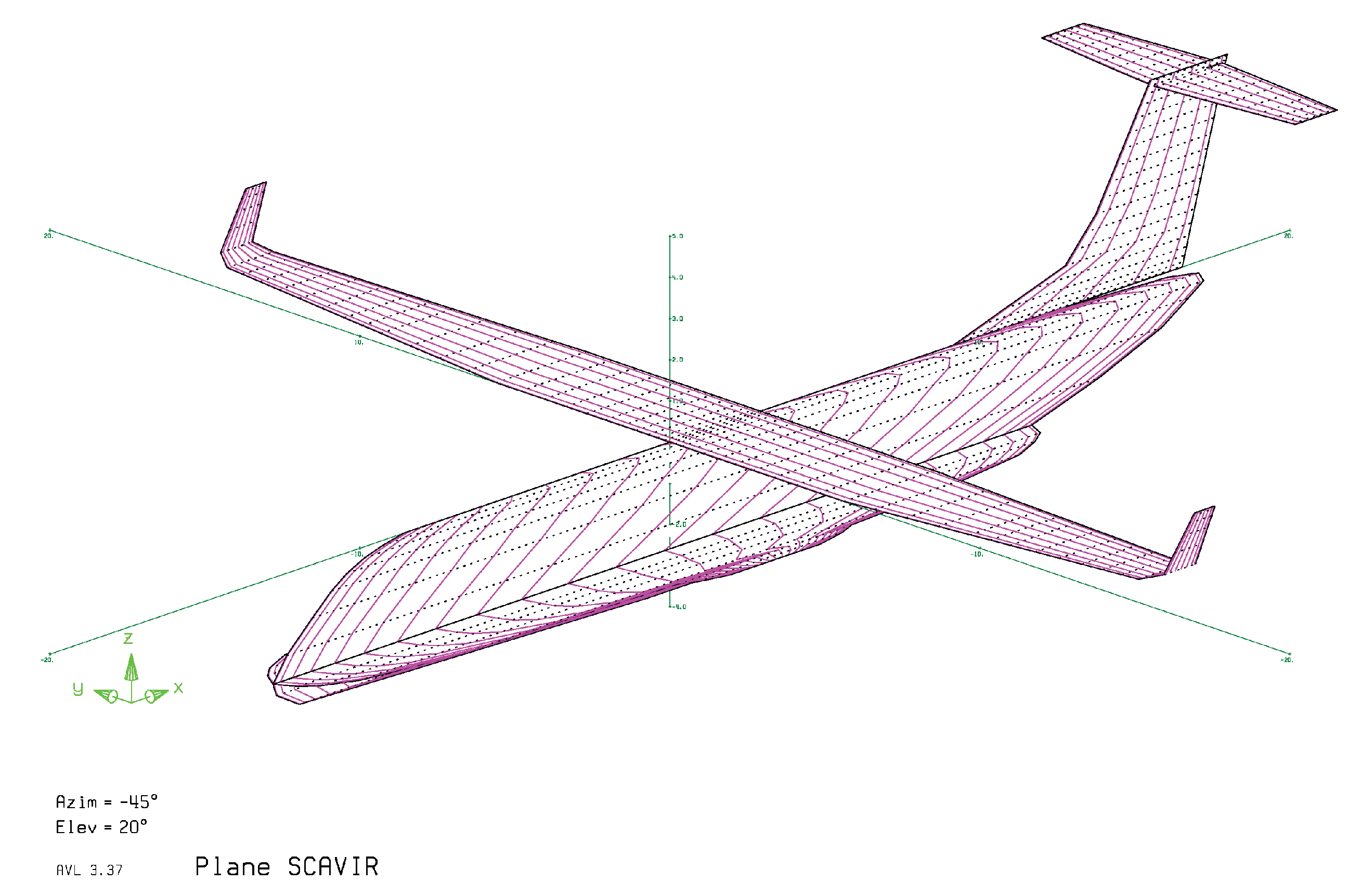
The reference VLM solution is obtained by employing the baseline model depicted in Figure 19, supplied with the proper definition of the trailing-edge control surfaces [22]. In Figure 20, the variation of the rolling moment coefficient against the lift coefficient is reported for both low and high-fidelity approaches. CFD predicts the loss in ailerons effectiveness for $C_L>0.9$, while VLM is not able to predict it. The drag breakdown corresponding to the aircraft configuration with deflected ailerons is illustrated in Figure 21, where each contribution is expressed as a percent of the total value. Several aerodynamic properties of the ailerons can be evaluated based on the CFD database. For example, a particularly interesting parameter is represented by the adverse yawing effect, which is induced by the rolling motion of the wing. This is indicated by the adverse sign of the yawing moment due to rolling, and quantified by the derivative $\partial C_n/\partial {\delta }_a$. CFD calculations provide a value of $2.6\times {10}^{-3}$ rad${}^{-1}$ at zero AoA, and $1.6\times {10}^{-2}$ rad${}^{-1}$ for $\alpha =7.5^{\circ }$, for this parameter.

4.2.2. Elevators

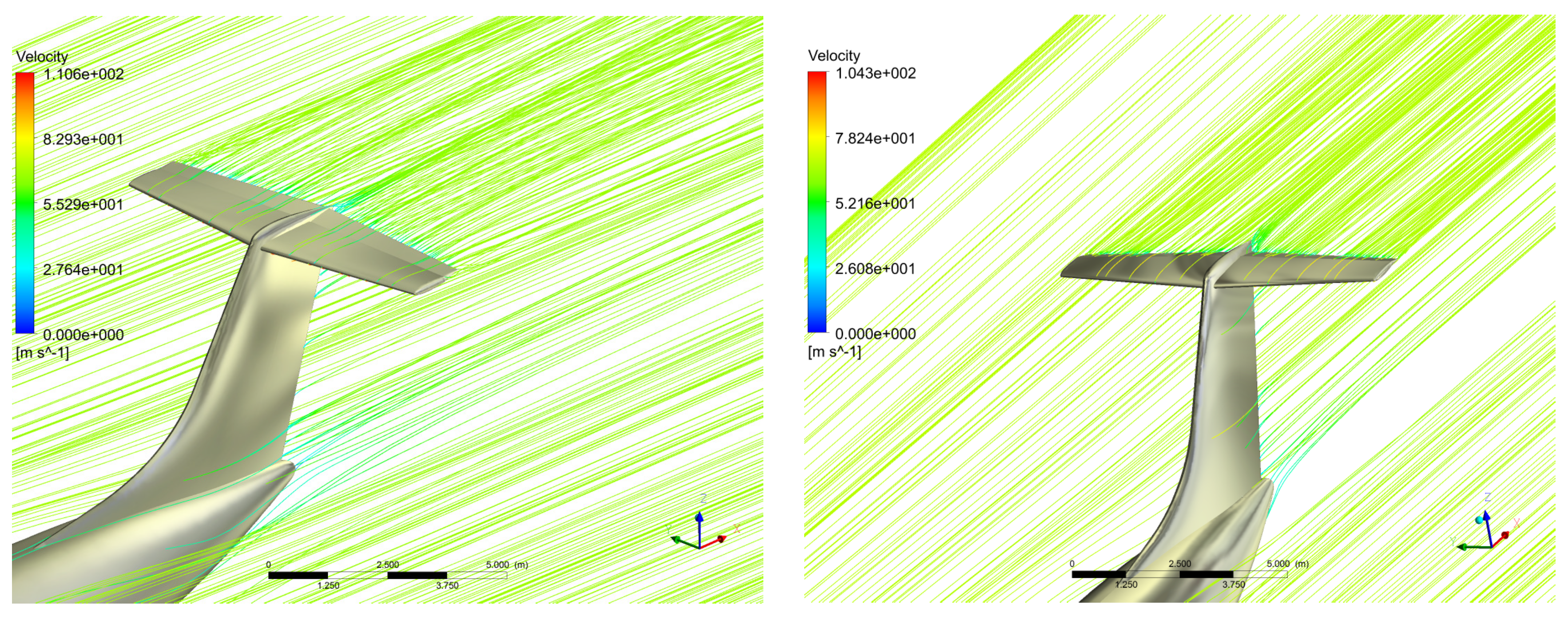
The aerodynamic properties of the elevators are presented for two different deflection angles that are ${\delta }_e=\pm {10}^{\circ }$. The air flow around the rear part of the aircraft is illustrated in Figure 22, where the streamlines are drawn for the configuration at zero AoA. The mean flow results in being not separated for both deflections, as is confirmed by looking at the corresponding half-span planar views, which are drawn in Figure 23.

The spanwise loading distribution on both aircraft wing and horizontal tailplane, for the flight condition at $M_{\infty }=0.2$, is shown in Figure 24 (left side). The maximum load on the horizontal tailplane occurs away from the symmetry plane, due to the presence of the vertical fin. The load on the horizontal tailplane decreases with the Mach number, as illustrated on the right side of the same figure. The variation of the pitching moment coefficient against the AoA is reported in Figure 25. When the elevator is not deflected (${\delta }_e=0^{\circ }$), apparently, the horizontal tailplane provides a negative lift that corresponds to $C_m>0$, for almost all AoA. This is due to its negative incidence with respect to the aircraft centerline ($i_h<0$), along with the downwash effect from the aircraft wing. Deflecting the elevator by $-{10}^{\circ }$ (upward) increases the absolute value of the negative lift. On the other hand, deflecting the elevator by $+{10}^{\circ }$ (downward) provides a positive lift, which gives in absolute value lower loading on the horizontal tailplane.

The variation of the pitching moment coefficient, for instance, at ${\delta }_e=+{10}^{\circ }$, for $M_{\infty }=0.2$ and zero AoA, is equal to $\Delta C_m=-0.54$. This result is comparable to the value obtained using a semi-empirical method, which is $-0.61$ [21]. The agreement is even better when making a comparison with the initial estimation made by industrial aerodynamicists in the pre-design phase of the new aircraft under development. When making the same analysis for the increment of the lift coefficient, it holds $\Delta C_L=0.109$, while the semi-empirical method provides the value of $0.1$ for the same parameter. Again, this estimation is consistent with the preliminary value found by the industrial partner. The more loaded configuration at ${\delta }_e=-{10}^{\circ }$ is further analyzed considering the associated drag polar in Figure 26, where an important increment for $C_{D0}$ with respect to the clean configuration, corresponding to 78 drag counts, is apparent. By looking at the associated drag breakdown, which is reported in Figure 27, it is interesting to note that the negative deflection of the elevators leads to higher drag for both fuselage body and vertical tailplane.

Finally, as far as the comparison with the VLM solution is concerned, the discrepancy of the results achieved with the two different methods is meaningful. This is likely due to differences in the modeling geometries that are employed, as was also found in similar works [30].

5. Conclusions

The present study must be intended as the proof-of-concept, namely the initial development of a CFD based procedure for predicting the aerodynamics of the flight control system of a mid-range commercial aircraft. Differently from similar works on the aerodynamics of aircraft control surfaces, where CFD results were often obtained for generic geometries, this study deals with models directly derived from real geometries provided by an aeronautical manufacturer. Several calculations have been performed with the aim of demonstrating the practical potential of the proposed methodology, which makes use of relatively coarse meshes, during the preliminary design procedure of a new regional transport aircraft under development. The good agreement with the wind-tunnel data for similar aircraft models is demonstrated. When compared against preliminary industrial data, which cannot be explicitly reported, the present computational results were considered fully acceptable by the industrial aerodynamicists. The computational analysis of the main trailing-edge control surfaces that is performed results in being reliable and valid, with a reasonable computational cost. The latter requirement is preferred, rather than the high accuracy of the results, owing to the character of the present study. Practically, it is demonstrated that the present CFD modeling can be effectively taken as a part of the industrial pre-design process, since it results in being accurate and affordable. A complete aerodynamic CFD database could be generated, given the prototypical geometry of the different control surfaces, in the pre-design industrial process. There remains the possibility of developing more sophisticated computational models for particular purposes, depending on the level of accuracy that is required, and the available computational resources.