Pulsed Blowing Interacting with a Leading-Edge Vortex

Abstract

Manipulation of vortex instabilities for aerodynamic performance increase is of great interest in numerous aeronautical applications. With increasing angle of attack, the leading-edge vortex of a semi-slender delta wing becomes unsteady and eventually collapses, endangering the flight stability. Hence, active flow control by pulsed blowing stabilizes the vortex system, enlarging the flight envelope for such wing configurations. The most beneficial outcome is the reattachment of the separated shear layer during post-stall, contributing to a lift increase of more than 50%. In contrast to high power consuming brute-force actuation, manipulating the flow instabilities offers a more efficient alternative for mean flow field control, which has direct repercussions on the aerodynamic characteristics. However, the flow mechanisms involving jet–vortex and vortex–vortex interactions and the disturbance convection through the flow field are little understood. This paper reports on the unsteady flow field above a generic half delta wing model with a $65°$ sweep angle and its response to periodic blowing. Numerical and experimental results are presented and discussed in a synergistic manner.

1. Introduction

Vortices are three-dimensional coherent flow features that occur very often in nature, as well as in many relevant technological applications. Hence, the manipulation of such brings great benefits. Depending on the desired outcome, the vortices can be destabilized or stabilized. Vortex premature decay is relevant for enhanced mixing in combustion chambers or destruction of tip/wake vortices for aeronautical safety requirements. However, sustaining the leading-edge vortices is desired for aerodynamic performance increase of swept wing configurations (e.g., delta wings). In [1], the authors identified three vortex types based on their applications: tip vortices, leading-edge vortices, and wake vortices, and discussed relevant vortical flow phenomena (edge separation, vortex roll-up, vortex instabilities, and vortex interactions) and corresponding control parameters (swirl angle, pressure distribution, location of disturbance injection, frequency). Control methods targeting the manipulation of each flow feature discussed were assessed in the paper mentioned. Irrespective of the actuator type (fluidic, moving-surface, or plasma actuator), the control mechanism either adds or removes vorticity, momentum, or turbulence [1].

Despite the additional external energy input, active flow control is superior to passive flow control, as on the one hand, it can be deployed on demand, and on the other, is able to trigger flow instability growth or decay by means of frequency conditioning. Local flow instabilities excited by periodic flow disturbance are an efficient way to alter the mean flow state in comparison to steady flow disturbance. In order to control the mean vortex system effectively, the physical processes involving vortex instabilities need to be understood [2,3,4].

Depending on the sweep angle, lift increase above delta wings is achieved by delaying vortex breakdown for slender planforms (leading-edge sweep angle of $\phi \ge 65°$) and by reattaching the shear layer for non-slender wings ($\phi \le 55°$). Therefore, various mechanisms are investigated, including passive vortex interactions, moving surfaces, blowing/suction, unsteady excitation, and others [4,5]. Occurring at sufficiently high angles of attack, the vortex breakdown is still a not fully understood vortex instability that manifests abrupt core deceleration, expansion, and pressure rise. There are two types of breakdown above delta wings, the spiral and the bubble type. The former type, the more common instability type for delta wings, shows a characteristic winding of the core, known as helical-mode instability [6,7].

Mitchell and Deléry presented a historical review of breakdown control methods, either by manipulating the vortex structure/location or delaying the breakdown location [5]. The two main parameters responsible for vortex breakdown are the swirl angle and the external pressure gradient. Hall demonstrated that the instability occurs when the swirl angle reaches $\varphi =arctan({\overline{u}}_{\theta }/{\overline{u}}_x)=50°$ [8]. Hence, continuously injecting fluid along the vortex core leads to reduction of the swirl angle and adds axial momentum, making the core flow more resistant to the adverse pressure gradient, as demonstrated on a $70°$ swept delta wing [5,9]. Because continuous blowing requires multiples of energy input and a continuous fluid supply compared to unsteady (periodic) fluid injection, the unsteady technology is more likely to reach application. On the same delta wing planform ($70°$), researchers conducted experimental [10,11] and complementary numerical investigations [5,12] on breakdown control by periodic sinusoidal blowing/suction at the leading-edge. There are primarily two dimensionless control parameters that affect the flow field, the momentum coefficient $c_{\mu }$ and the reduced actuation frequency $F^{+}$, defined as:

$$c_{\mu }=\frac{{\rho }_j\overline{{u^{\prime }}_j^2}{A}_j}{1/2{\rho }_{\infty }{U}_{\infty }^2{A}_{wing}}$$

(1)

$$F^{+}=f·c_r/U_{\infty }.$$

(2)

In Equation (1), index “j” designates the jet variables (density ${\rho }_j$, mean squared jet velocity fluctuations $\overline{{u^{\prime }}_j^2}$, and slot area $A_j$) and index “∞” stands for the freestream values. In Equation (2), the frequency f is undimensionalized by the time of flight, the ratio of freestream velocity $U_{\infty }$, and a reference length, e.g., root chord $c_r$. According to smoke visualizations [10], these parameters offered maximum downstream shift of the breakdown delay at values of $c_{\mu }=0.45$% and $F^{+}$ = 1.2–1.4 (at a chord Reynolds number range of $Re=1-5.5\times {10}^5$). However, transient water-tunnel PIV investigations ($Re=2.5\times {10}^4$) indicate no vortex breakdown delay, but rather, a reduction of the wake by axial momentum increase downstream of breakdown [11]. It is pointed out that with forcing, the breakdown location fluctuates longitudinally, making its detection difficult. The numerical modeling of the unforced and forced vortical flow field validated the findings and demonstrated the advantages of combining experimental and numerical investigations [13]. The results showed the generation of a strong shear layer vortex during the blowing phase that enhanced momentum transport into the primary structure. While the breakdown location remains rather unaffected, axial velocity increases near the surface, increasing suction and thus the normal force. The periodic forcing leads to an elliptical trajectory of the vortex core in a crossflow plane.

Tangential blowing/suction at the leading-edge of a $75°$ swept delta wing model successfully delayed breakdown at an incidence angle of $\alpha =54°$ (at which the vortex bursts near the apex) [14]. Alternating blowing/suction ($c_{\mu }=0.36$%, $F^{+}=1.3$) generated the most downstream displacement of breakdown $\Delta x/c_r=0.46$ compared to steady suction or blowing. In addition, the transient response of the breakdown location based on smoke visualization revealed a long term hysteresis effect, also reported on a pitching delta wing [15].

Oscillating piezoelectric membranes operated with high resonance frequency are used to generate sinusoidal blowing/suction in five segments distributed along the leading-edge of a $60°$ delta wing [16]. The pure sine wave signal failed to improve the stalled flow field, while adding low frequency signal modulation ($F^{+}=\mathcal{O}\left(1\right)$) led to significant stall delay. The burst mode signal demonstrated an optimum ($c_{\mu }=0.03$%, $F^{+}=1.0$) in efficiency, outperforming the amplitude modulated actuation ($c_{\mu }=0.4$%, $F^{+}=2.0$). This result showed the strong dependency of the shear layer receptivity to different actuation signals. The dynamics involving the shear layer manipulation over a delta wing is analogous to 2D separation, which is discussed briefly below.

Control of separating 2D layers proves most effective when periodic disturbances are injected in the separating shear layer in a frequency range that triggers inherent instabilities (Kelvin–Helmholtz) [3]. Naturally, the shear layer separating from the sharp leading-edge of a delta wing becomes unstable, generating discrete vortices that induce the shear layer roll-up into the primary vortex [17]. Reordering the discrete vortices increases the curvature of the mixing sheet, leading to a reduction of the separation region or even to flow reattachment [4,5,18]. The lowest disturbance amplitudes $c_{\mu }$ are required if the reduced actuation frequency is adjusted to $F^{+}=\mathcal{O}\left(1\right)$. This generates large coherent structures that generate maximum momentum transport across the shear (mixing) layer [3].

The current paper reports on the effect of pulsed blowing at the leading-edge of a sharp edged generic delta wing with a $65°$ sweep angle. In contrast to previously discussed leading-edge vortex control studies, the actuation consists of valve controlled pulsed blowing. Kölzsch proved the delay in vortex breakdown when the control frequency is tuned to the helical-mode instability [19]. In a subsequent experimental investigation, the effect of pulsed blowing on the velocity field and aerodynamic characteristics was validated [20]. Furthermore, the timing of the distributed blowing jets was altered in order to study the influence of phase and frequency modulation on the flow field. This demonstrated that synchronized blowing alters the flow field the most. Hence, quasi-2D disturbances achieved a maximum momentum transport across the shear layer compared to 3D disturbances, as also reported in [3,16]. Those experimental findings are complemented in this paper by detached eddy simulations (DES) at three flow regimes around stall (corresponding to angles of attack of $\alpha =23°,35°$, and $45°$). The different actuation type and experimental setup between the present work and [16] show how the flow response is more dependent on the amplitude and frequency (which is universal) than on the jet form and direction. Based on both non-intrusive methods, computational fluid mechanics (CFD) and particle image velocimetry (PIV), the results are analyzed and discussed in a synergistic fashion, focusing on the interaction between pulsating blowing jets and the vortical field. Hence, the advantages of both methods are exploited: for example, analysis of the regions in PIV planes contaminated by reflections (near-wall region) is conducted more effectively based on numerical results.

2. Methods

2.1. Delta Wing Model

The half delta wing model representing the Vortex Flow Experiment 2 (VFE-2) geometry was equipped with 12 pressure chambers distributed in three segments inside the $65°$ swept, sharp leading-edge, as sketched in Figure 1a and reported in [19,20]. Each chamber was supplied by pressurized air through a two state (open/closed) operating valve. The chambers, valves, and pressure tubes were integrated inside the half-wing model. The outlet of the pressure chamber represented a pair of high aspect ratio slots (2 mm × 10 mm) angled at 45$°$ to the leading-edge and $90°$ to each other. Opening the valve at the chamber’s inlet filled the chamber with air at higher pressure than in the environment. The pressure difference led to the generation of two discrete jets functioning as fluidic vortex generators. The valve switching time between closed and open state adjusted the phase and frequency of a periodic blowing signal (investigated here). The slot exit velocity $u_j$ could be adjusted merely segment-wise and increased monotonically with the supplied air pressure. Such a design allowed infinite possibilities for actuation signals. However, in the current investigation, all 12 actuator pairs were operated synchronously, representing a periodic quasi-2D disturbance injection at the leading edge.

Figure 1b shows the time records of the normal and tangential velocity component above a slot in quiescent air conditions ($U_{\infty }=0$) operating at a frequency of $f=12$ Hz and a duty cycle of $DC$ = 25%. The negative sign of the vertical velocity component $v_j$ indicated that the elongated jets were directed normally to the wing’s suction side and slightly inboard. Throughout these investigations, the fluidic actuators produced this kind of periodic (pulsating) velocity signal ($DC$ = 25%), but with the frequency tuned to the targeted flow instabilities.

2.2. Experimental Setup

The wind-tunnel tests were conducted in the low speed wind-tunnel facilities of the Chair of Aerodynamics and Fluid Mechanics (Technical University of Munich). The cases investigated included three angles of attack: prior to stall ($\alpha =23°$), at stall ($35°$), and beyond stall ($45°$). For all the measurements, two freestream velocity values were set, $U_{\infty }=$ 12 m/s for both highest angles of attack and 24 m/s for the lowest, corresponding to a Reynolds number based on the mean aerodynamic chord ($l_{\mu }=0.651$ m) of $Re=0.5$ and $1.0\times {10}^6$, respectively. For each freestream condition investigated, both the unforced and forced flow field were measured. For the actuated cases, the optimal control parameters were tuned to the addressed instabilities [19] and lied in the range reported by numerous other studies (cf. Section 1). The test cases are summarized in

Table 1. Test cases with corresponding control and numerical parameters.

Test Case	$\mathit{\alpha }$	${\mathit{U}}_{\mathbf{\infty }}$	$\mathbf{Re}$	f	${\mathit{F}}^{+}$	${\mathit{c}}_{\mathit{\mu }}$	$\mathbf{\Delta }\mathit{t}$	$\mathit{\tau }$	CFL
Vortex breakdown	$23°$	24 m/s	$1.0\times {10}^6$	65 Hz	2.6	0.14%	$1.9\times {10}^{-5}$ s	$5\times {10}^{-4}$	0.2
Stalled flow	$35°$	12 m/s	$0.5\times {10}^6$	32 Hz	2.6	0.55%	$3.9\times {10}^{-5}$ s	$5\times {10}^{-4}$	0.2
Post-stall	$45°$	12 m/s	$0.5\times {10}^6$	12 Hz	1.0	0.85%	$1.0\times {10}^{-4}$ s	$1\times {10}^{-3}$	0.5

.

Stereoscopic PIV measurements of the complete flow field were conducted on all cases with the setup reported also in [20]. A double laser pulse with an energy of 325 mJ and a wavelength of 532 nm illuminated particles dispersed in the fluid at two consecutive time instances. The instant three component velocity field in the measured plane was calculated based on the cross-correlation technique. Each plane was scanned 400 times with a frequency of 13 Hz. Crossflow scanning was synchronized with the blowing frequency for additional phase averaged information. The work in [20] showed that the synchronous blowing had the greatest influence on the flow field. Yet, the reason for this lied in the jet–vortex interaction and consecutive discrete vortex pairing. In order to investigate this, time/scale resolving numerical investigations complemented the time/phase averaged experimental results. The PIV uncertainty of the mean values, which was calculated based on the correlation statistics method [21], was highest in the vortex core and in the breakdown region, but did not exceed 2.5%$U_{\infty }$ in all three components. Phase averaged crossflow investigations showed local uncertainty peaks below 3.8%$U_{\infty }$ above the blowing slots and during the blowing phases.

2.3. Numerical Setup

Detached eddy simulations (DES) of the unperturbed and perturbed flow field were solved in ANSYS Fluent for each of the three investigated angles of attack ($\alpha =23°$, $35°$, and $45°$) under incompressible flow assumptions ($Ma<0.2$). DES is a hybrid RANS/LES model that combines the low computational requirements of RANS in stable flow regions and boundary layers and the scale resolving advantages of LES in unsteady flow regions. The momentum transport equations were closed with the shear stress transport (SST) equations, of the turbulent kinetic energy k and the specific dissipation rate $\omega$. The additional factor in the turbulent kinetic energy (TKE) dissipation term, the DES-TKE-multiplier $F_{DES}$, switched from SST-RANS to LES when $F_{DES}>1$. In the original formulation, turbulence was resolved if the modeled turbulent length scale $L_t$ exceeded the maximum element edge multiplied by a calibrated constant $C_{DES}{\Delta }_{max}$ ($C_{DES}=0.78$) [22]. Additional wall shielding (already implemented in the switching function of the SST formulation $F_{SST}$) restricted the protrusion of LES in the boundary layer that caused unphysical grid induced separation [23]. The multiplier is defined in Equation (3) and its distribution in the delta wing flow field displayed in Figure 2.

$$F_{DES}=max\left(\frac{L_t}{C_{DES}{\Delta }_{max}}(1-F_{SST}),1\right)$$

(3)

The SIMPLEC (Semi-Implicit Method for Pressure Linked Equations - Consistent) algorithm couples the pressure with the velocity for the pressure based solver. The gradients are evaluated with the least squares cell based algorithm. Momentum and pressure advection schemes are second-order accurate, whereas the turbulence advection scheme is first-order upwind, which should be accurate enough regarding the dominance of the source terms in both turbulence transport equations [24].

Initialized with the converged steady RANS solution, the DES computations progressed in time using a dual time stepping approach with the bounded second-order implicit scheme. The length of a time step was test case dependent, but its definition universal: it represented a division of 1/800 of one blowing period ($T=1/f$). For each case investigated, Table 1 lists the corresponding time step length $\Delta t$ and its non-dimensional form, relative to the convective time scale $\tau =\Delta t/(c_r/U_{\infty })$. The corresponding Courant–Friedrichs–Levy (CFL) number did not exceed one, which was the recommended value for LES [24].

The flow field around the delta wing was computed in a $15c_r\times 5c_r\times 15c_r$ large domain [25]. The simulations modeled the half-flow problem by attributing a symmetry boundary condition at the wing root. The delta wing was positioned $5c_r$ away from the inlet (in front and below) and the opening (sideways). The outlet planes were located two times farther downstream than the inlet planes, for sufficient convergence of the large high angle of attack wake towards freestream conditions. The fluid domain was discretized in a block structured manner using the meshing software ANSYS ICEM. The grid sensitivity study of the $\alpha =45°$ case concluded that the medium sized grid (49 million hexahedron cells) offered sufficient accuracy [25]. Overall, the grid generation conformed to the flow regions reported in [26]. The forcing was modeled by pulsating wall velocity at the actuator exit planes (red surfaces in Figure 3a).

The surface mesh of the wing had Y shaped blocking with 411, 408, and 525 elements distributed along the root chord, the trailing edge, and leading-edge, respectively (Figure 3). The maximum edge length of the surface mesh read $\Delta =0.0024c_r$. Towards the leading-edge where high gradients and flow separation were present, the area of the surface elements decreased, as shown in Figure 3a. The volume around the delta wing was divided into four O-grid layers (Figure 3b), permitting variable wall-normal element growth. The elements nearest the wall had a height of 0.01 mm, resulting in a wall distance of $y^{+}$ below unity over almost the entire wing surface. Away from the wall, the elements grew exponentially with a factor of 1.13 within the first O-grid, located in the boundary layer. In the outer layers, the second and third O-grid, the growth factor was reduced to 1.04, generating a region with good quality elements, required for LES (focus region). The last O-grid layer was located in the departure region where the element spacing increased towards the Euler region [26].

Table 2. Wall-normal grid parameters.

Flow Region	O-Grid Layer	Layer Thickness	Minimum Cell Spacing	Growth Factor
Viscous region	1st	3 mm	0.01 mm	1.13
Focus region	2nd	27 mm	0.48 mm	1.04
Focus region	3rd	190 mm	1.30 mm	1.04
Departure region	4th	300 mm	6.10 mm	1.20

summarizes the grid parameters.

3. Results and Discussion

Before the effect of actuation is analyzed, the baseline transient flow field is presented and discussed based on the PIV and DES results. All three cases investigated showed particularities and different dominant instabilities. At $\alpha =23°$, the vortex broke down at chord station $x/c_r\approx 0.60$ above the wing. At stall ($\alpha =35°$), the breakdown location reached the apex region. Increasing the angle of attack beyond stall led to an abrupt vortex collapse at $41°<\alpha <42°$ [20], resulting in massive lift loss. Hence, the third investigated baseline case was comprised of the non-reattaching shear layer at $\alpha =45°$.

3.1. Vortex Breakdown

The breakdown location was mainly dependent on the sweep and incidence angle. For a $65°$ sweep delta wing, breakdown occurred at the trailing edge at $\alpha \approx 20°$ and progressed upstream with increasing angle of attack. The adverse pressure gradient along the core constituted an internal (caused by swirl and stream tube divergence) and an external portion, which influenced the breakdown location [8]. When the longitudinal momentum equaled the adverse pressure, the core flow stagnated, followed by a typical winding and dissipation to turbulence. Hence, breakdown was described by the change in sign of the axial velocity and axial/lateral vorticity. However, the breakdown location was very unsteady, describing oscillatory movement with significant amplitudes as demonstrated by two images of the vortex core visualized by smoke in Figure 4. In this paper, the classical definition of the breakdown location as a constantly fluctuating point of stagnation was replaced by a mean breakdown location correlated with a maximum TKE region.

Figure 5 shows the measurement plane cutting horizontally along the vortex core capturing the breakdown phenomenon occurring at $\alpha =23°$ (first investigated case). The PIV results (a,b) were compared to equivalent DES results (c,d), however at translated positions by $\Delta x/c_r=\Delta y/s=0.1$ due to a delay in the CFD predicted breakdown (see Section 3.4.1). Included in Figure 5a,c, the distribution of the averaged axial velocity related to the freestream velocity $U_{\infty }=24$ m/s demonstrated that breakdown transitions the flow from a jet-type to a wake-type flow. The transition region showed high concentrations of turbulent kinetic energy caused by the fluctuations of the stagnation/breakdown point. The unsteady region ($k/U_{\infty }^2\ge 0.1$) expanded downstream around the low energy core (relative axial velocities of $u/U_{\infty }<0.5$). The flow unsteadiness downstream of breakdown was generated by the core flow dissipating into discrete vortices.

The instantaneous distribution of the dimensionless in-plane vorticity ${\omega }_z(l_{\mu }/U_{\infty })$, related to the ratio of the freestream velocity to the mean aerodynamic chord, identified the discrete vortices contained in the shear layer and in the breakdown wake (cf. Figure 5b,d). The wake flow included reversed flow regions, enclosed by $u/U_{\infty }=0$ isolines. The wake vortices were ordered in pairs and convected downstream in a helix path before dissipating into turbulence. Alternating regions of positive (red) and negative (blue) in-plane vorticity in the shear layer evidenced vortex generation through the Kelvin–Helmholtz instability. The shear layer vortices spiraled around, eventually transporting vorticity into the primary vortex core.

Figure 6 shows the instantaneous computed vortex cores designated by the isosurface of the Q-criterion $Q={10}^5$ s${}^{-2}$. The color bar is scaled with the relative axial velocity in the range $-0.5\le u/U_{\infty }\le 2$. Upstream of breakdown, the stable vortex core had high axial velocities and showed small wave patterns. The shear layer was unstable, forming stationary vortices that spiraled around the main structure. Such vortices were also measured above a $70°$ delta wing and reported in [27]. The breakdown position was evidenced by the abrupt core dilatation and disintegration into smaller vortices that increased turbulence. The abrupt deceleration of the primary structure correlated to pressure increasing downstream. The secondary vortex, which was located between the primary vortex and the leading-edge, broke down upstream of the primary vortex breakdown location. This then led to detachment of shear layer vortices interacting downstream with the wake flow.

3.2. Stall

At ${\alpha }_{max}=35°$, the vortex broke down near the apex, as suggested by the mean axial velocity and vertical vorticity distribution in the measured core plane presented in Figure 7. In contrast to the lower angle of attack, the wake-type flow dominated the suction side and revealed reversed mean flow in its core (cf. Figure 7a,c). At $\alpha =35°$, the external pressure gradient was greater than at $23°$, promoting flow instabilities that generated the formation of discrete vortices in the wake (as presented in the core plane of the flow field in Figure 7b,d). It was evident that the breakdown region was dominated by dipoles of vertical vorticity along the vortex core upstream of $x/c_r=0.2$. From this region, where a strong interaction with the separated shear layer was present ($k/U_{\infty }^2>0.15$ in Figure 7a), clusters of positive vorticity and negative vorticity departed in a conical path around the reversed flow regions. The pairs of vorticity peaks with different signs at breakdown suggested the formation of the helical-mode instability.

At both angles of attack $\alpha =23°$ and $35°$, the numerical method predicted a farther downstream, $\Delta x/c_r=0.1$, and a more “violent” breakdown. The computed pre-breakdown region showed a very stable behavior compared to the measured flow field with increased core velocities, explaining the delayed breakdown. Downstream, the core flow in both methods decelerated towards similar mean values of $u/U_{\infty }$, and dimensionless TKE levels in the range $0.10<k/U_{\infty }^2<0.15$ predominated the breakdown wake. In consequence, the core flow decelerated more abruptly in the numerical simulations, which predicted as well a higher TKE peak correlated with the mean breakdown position.

Comparing the instantaneous distribution of in-plane vorticity between PIV and DES, the numerically predicted breakdown showed a higher core dilatation, evidenced also by the wider stagnation region. In addition, the core flow in the measurements was unsteady prior to breakdown with low fluctuations along the core with amplitudes of $|{\omega }_z(l_{\mu }/U_{\infty })|<50$. The DES predicted instead a steady core (without fluctuations). Despite the observed differences between experiments and computations that may be due to apex resolution and flow constriction by the symmetric boundary condition in CFD, the vortical unsteady flow field was well predicted. The aerodynamic coefficients are discussed in Section 3.4.

Analogous to the previous case, Figure 8 shows vortex cores based on the Q-criterion. The core of the primary structure was stable up to $x/c_r=0.3$, where it broke down, wound downstream about one period, and dissipated into turbulence. The shear layer instability generated vortices with a positive winding around the core. However, in the wake region $x/c_r>0.3$, shear layer vortices changed the winding direction. This was caused by the strong interaction of the unsteady wake of the primary vortex with the vortices shed from the leading-edge. The shear layer transported the shed discrete vortices around the burst vortex core. Throughout this process, the vortices interacted with the unsteady and highly turbulent wake, resulting in complex 3D structures with random orientation downstream.

3.3. Post-Stall

Figure 9 presents the wake-type flow field at $\alpha =45°$, in which the shear layer was not able to reattach on the wing’s upper surface. The region with dimensionless TKE $k/U_{\infty }^2>0.05$ dominated the shear layer, the confluence of the freestream flow, and the reversed low energy flow above the wing. Due to the shear layer instability, evidenced by the downstream increasing curliness of the isoline $u=0$, discrete vortices with negative vertical vorticity emerged (cf. Figure 9b). Similar to the cases discussed previously, the computational baseline flow field at $\alpha =45°$ showed a delayed and more accelerated development of shear layer instability compared to the measurements. By comparing Figure 9b,d, the computed shear layer needed a longer distance in order to become unstable and develop discrete vortices. Again, the view on the longitudinal plane was shifted relative to the PIV plane ($\Delta x/c_r=\Delta y/s=0.3$). This led also to delayed TKE development (cf. Figure 9c).

In Figure 10, the computational result revealed the leading-edge shedding mechanism. Driven by the shear layer instability, vortex separation was initiated upstream and continued downstream. Consequently, the axis of the vortices showed a downstream and downward inclination. Throughout the downstream transport process, the vortices became unstable along their axis and canted in the freestream direction.

3.4. Pulsed Blowing

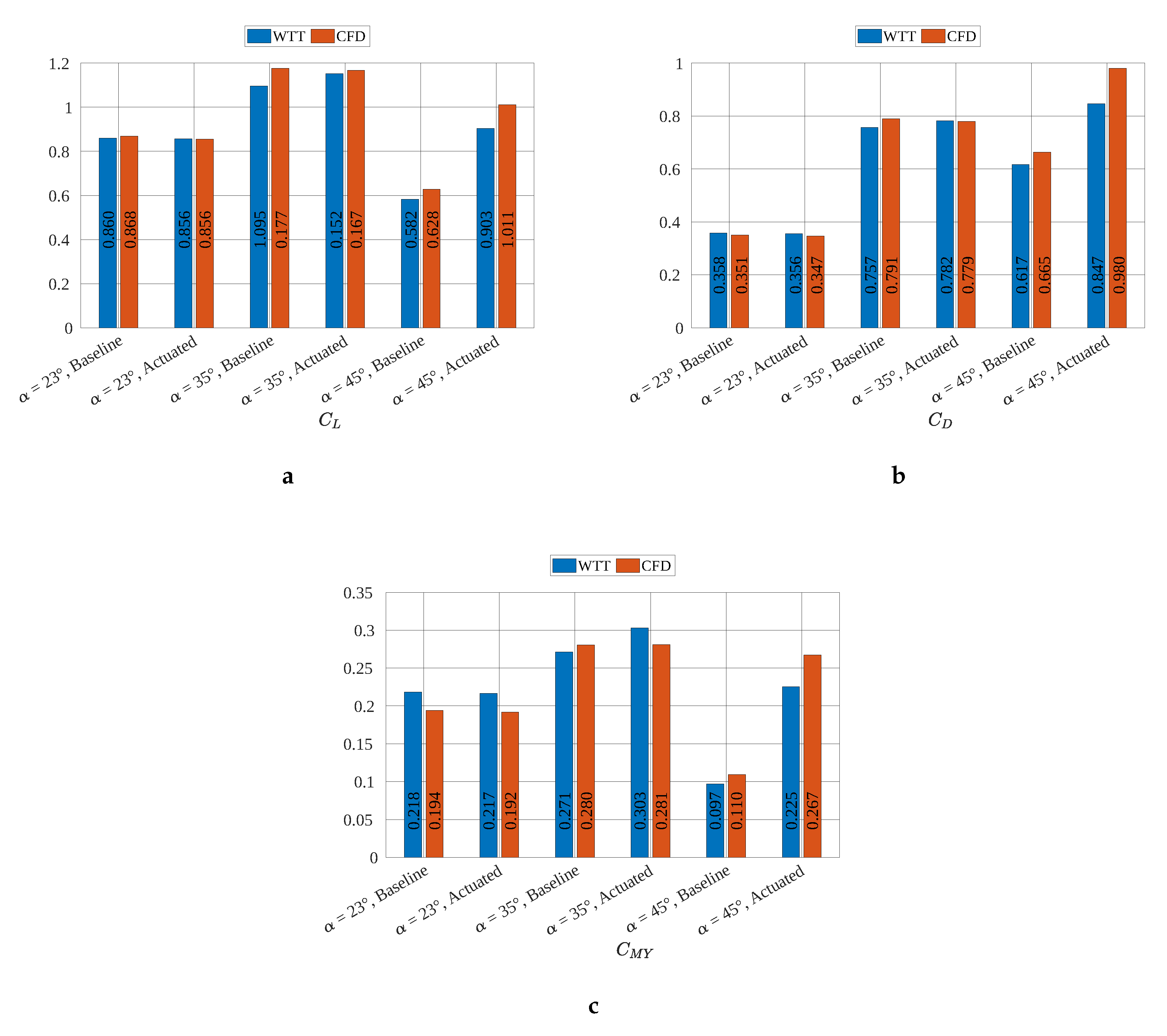
Based on the measured time and phase averaged velocity fields (PIV) and on the time accurate numerically solved velocity fields (DES), the current section discusses the effect of the applied periodic perturbation method on each flow field type. The mean aerodynamic coefficients, both from experimental measurements and from computed values, are assessed for each case investigated in Figure 11. The measurement uncertainty read $C_{L,err}=C_{D,err}=0.01$ for the lift and drag coefficient and $C_{MY,err}=0.003$ for the pitching moment coefficient [20]. With increasing angle of attack, the computed force and moment coefficients diverged from the wind-tunnel test (WTT) results. Two sources might affect this spread: no application of open-jet wind-tunnel corrections and vortex approaching the symmetry boundary with increasing angle of attack.

At $\alpha =45°$, the actuation reattached the shear layer, forming a sustained wake-type primary vortex structure, increasing the lift by more than 50%. For the lower investigated angles of attack $\alpha =23°$ and $35°$, at which a primary vortex structure was naturally present above the wing, pulsed blowing shifted the breakdown location downstream without significantly improving the integral aerodynamic coefficients. Based on the different flow types, vortex breakdown and wake flow, the actuation addressed different instabilities; therefore, the subsequent investigation attempted to describe the mechanisms leading to breakdown delay and shear layer reattachment.

3.4.1. Delay of Vortex Breakdown

When pulsed blowing was applied on the flow field dominated by vortex breakdown, the breakdown location was shifted downstream, depending on the angle of attack investigated. At $\alpha =23°$, PIV measurements along the core reported a mean delay of breakdown from $x/c_r=0.55$ to $0.58$ [20]. The DES method estimated the breakdown location too far downstream compared to PIV, for both the undisturbed ($x/c_r=0.66$) and disturbed flow field ($x/c_r=0.76$). At $\alpha =35°$, the mean axial stagnation point offered a more suitable criterion for measuring the effect of blowing on the conical wake region. According to the PIV investigations, pulsed blowing reduced the low energy region, displacing it downstream by a chord distance of $\Delta x/c_r=0.19$. Due to the symmetry boundary condition constricting the apex flow field, the undisturbed flow at the stall angle of attack stagnated farther downstream ($x/c_r=0.32$) compared to the experimental findings (0.24). Hence, the computed mean flow responded to actuation by a $\Delta x/c_r=0.13$ downstream displacement of the stagnation point.

Table 3. Relative chordwise positions $x/c_r$ of the breakdown ($\alpha =23°$) and stagnation location ($35°$).

	$\mathit{\alpha }=23°$		$\mathit{\alpha }=35°$
	Baseline	${\mathit{F}}^{+}=2.6$	Baseline	${\mathit{F}}^{+}=2.6$
PIV:	0.55	0.58	0.24	0.43
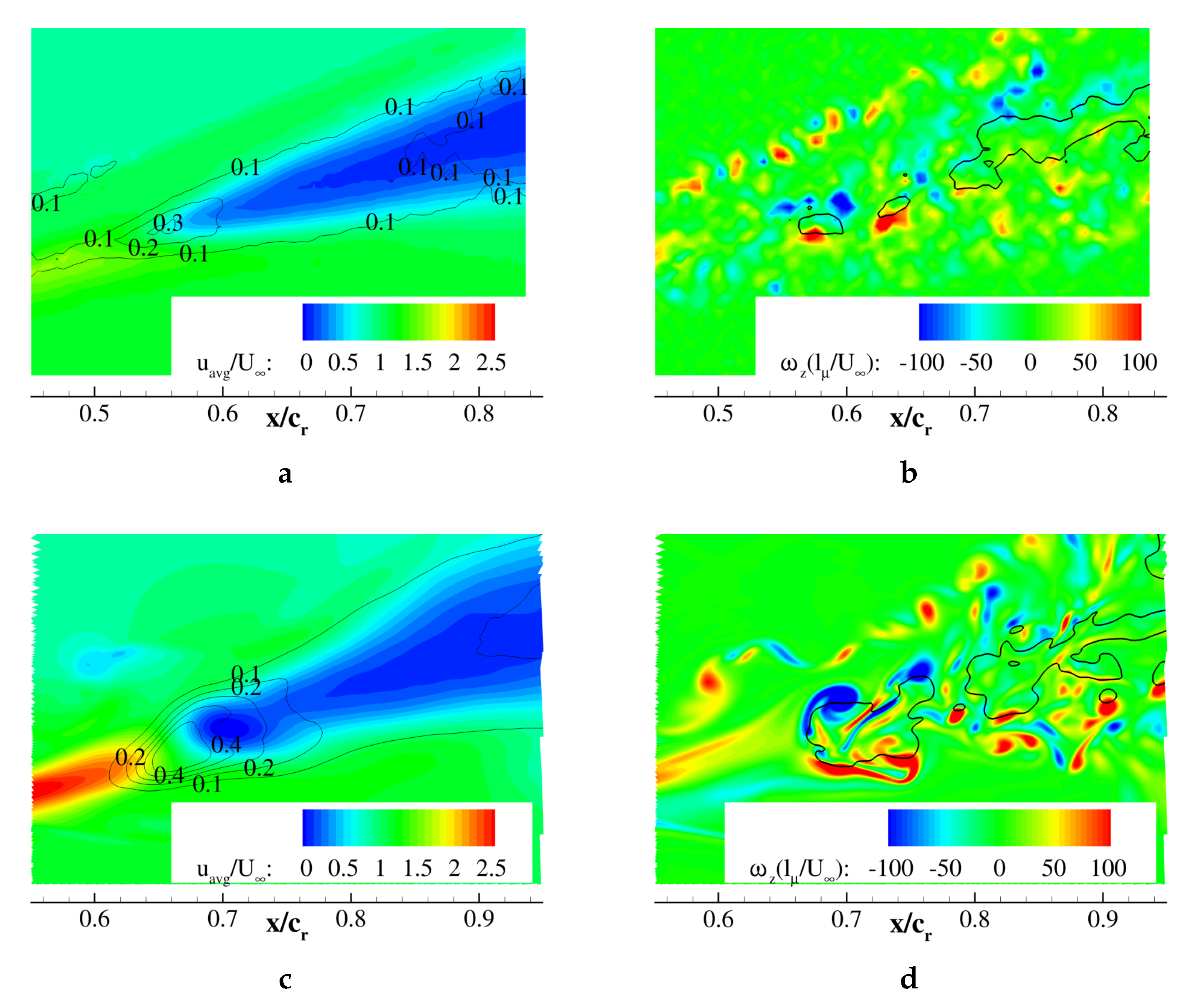
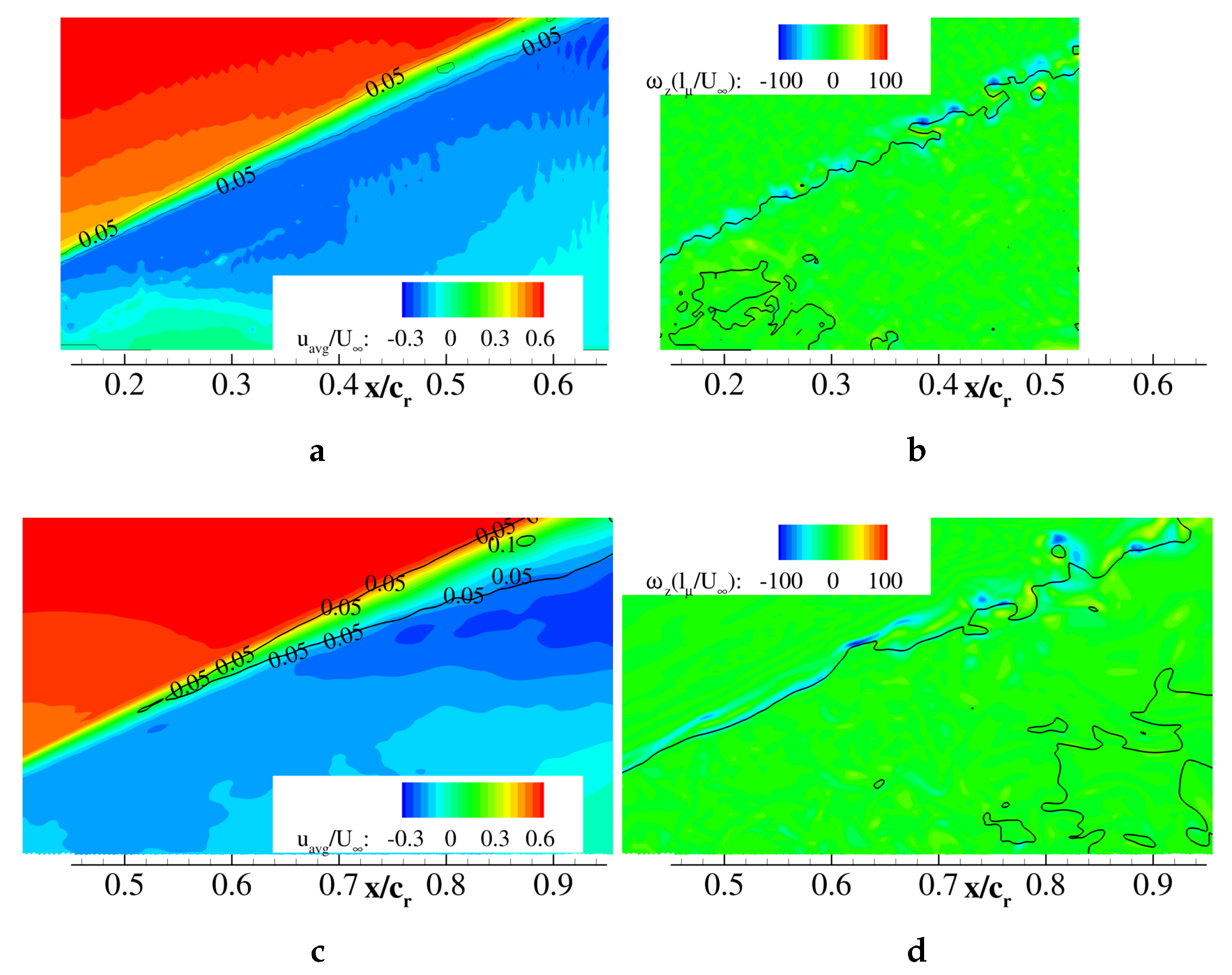
DES:	0.66	0.76	0.32	0.45

summarizes the computed and measured chordwise breakdown/stagnation positions based on the mean flow field. However, the average times between DES and PIV were largely unequal, in favor of the latter.

Figure 12 shows velocity profiles extracted from PIV crossflow planes across the vortex core for two angles of attack (a) $\alpha =23°$ and (b) $35°$. The effect of pulsed blowing was evidenced by assessing the baseline and the actuated velocity profiles. For the purpose of completeness, two chordwise locations were investigated. In Figure 12a, the full and dashed lines represent the spanwise velocity distribution upstream ($x/c_r=0.50$) and downstream (0.70) of breakdown, respectively. Between these planes, the core flow transitioned from a jet-type (black line) to a wake-type flow (black dashes) with a decrease in swirl (blue graphs). Actuation had a minor effect in the pre-breakdown region, reducing both u and w (red and green) by a small amount. However, downstream of breakdown, pulsed blowing reduced the wake significantly and increased the gradient $\partial w/\partial y$ in the core, suggesting an increase in swirl compared to the unactuated case.

At stall, wake flow was measured even at $x/c_r=0.15$ (cf. Figure 12b). The similarity of the cross-sectional velocity profiles downstream of breakdown for both angles of attack $\alpha =23°$ ($x/c_r=0.70$) and $\alpha =35°$ ($x/c_r=0.15$) revealed that pulsed blowing had a major influence on the flow region downstream of breakdown. The manipulation of the shear layer vortices by pulsed blowing increased the momentum transport in the radial direction with respect to the vortex axis. The actuation method was effective merely on the unstable vortex region, downstream of breakdown. For this reason, the flow field at $\alpha =35°$ was more affected than at $23°$ (cf. Table 3).

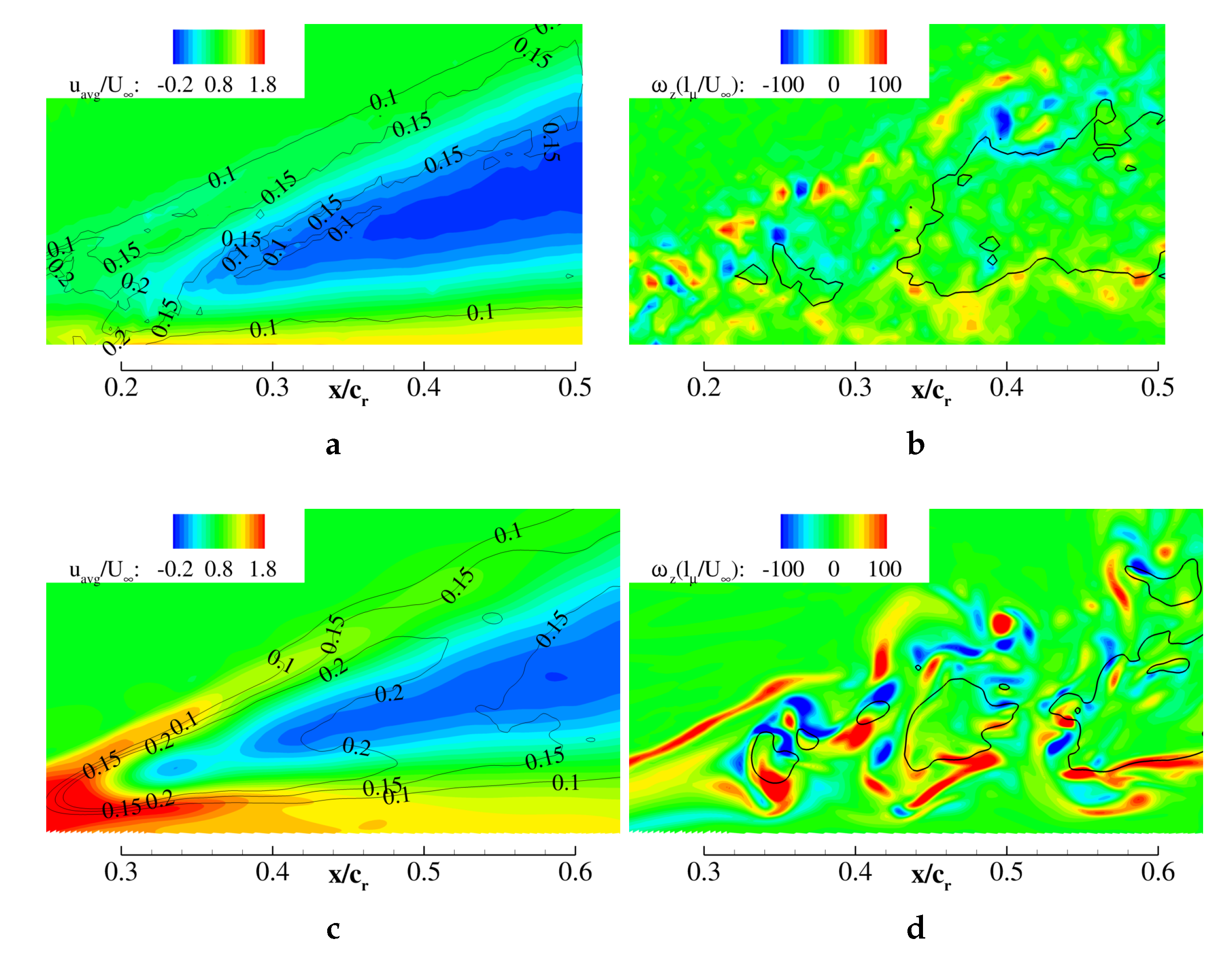
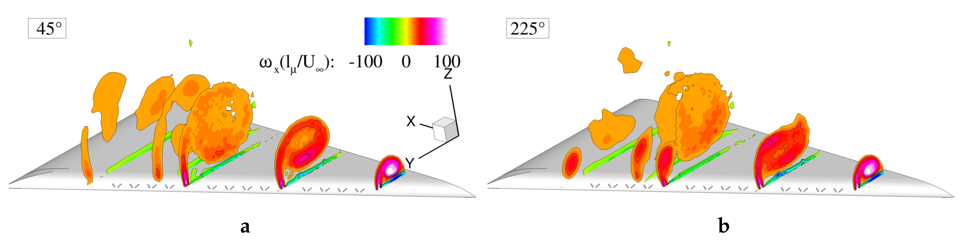
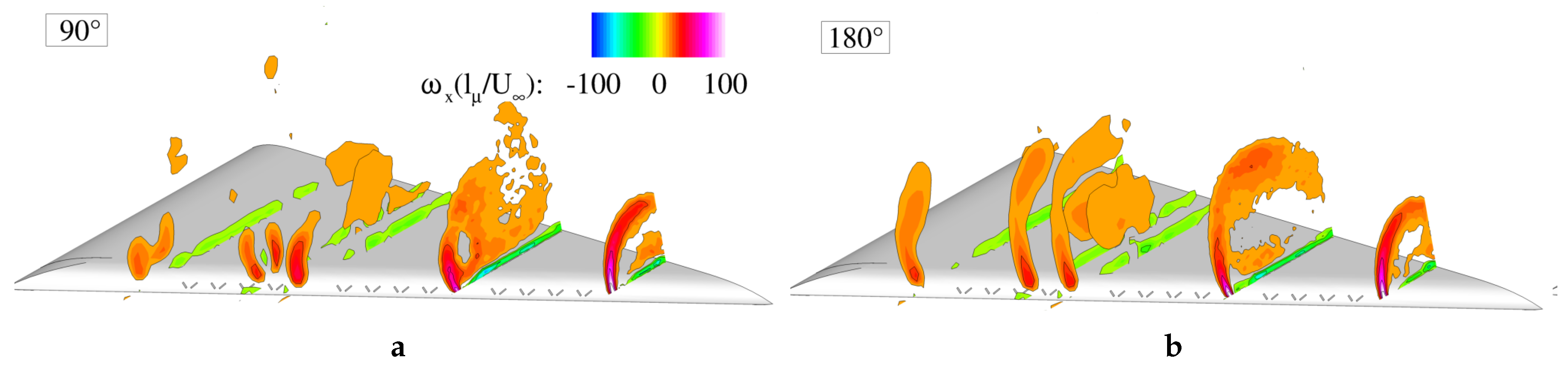
Crossflow phase averaged axial vorticity distribution extracted, during (Figure 13a) and $T/2$ after blowing (b), showed the mean periodic trajectory of vorticity peaks. During blowing, the vorticity distribution resembled the averaged flow field. At $x/c_r=0.2$, the vortex was stable with a jet-like topology. This region was rather unaffected by the disturbance injected downstream. Instead, the post-breakdown region showed a periodic movement initiated by the excitation. After half of a period, expressed also as a phase angle delay of $\Delta \theta =180°$, strong shear layer vortices were generated along the leading-edge. These were responsible for the roll-up process and the enhanced momentum transport across the shear layer.

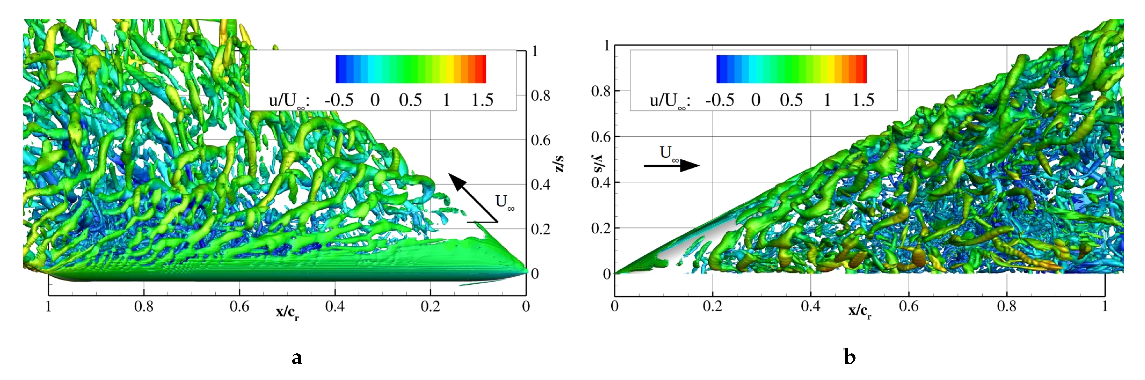
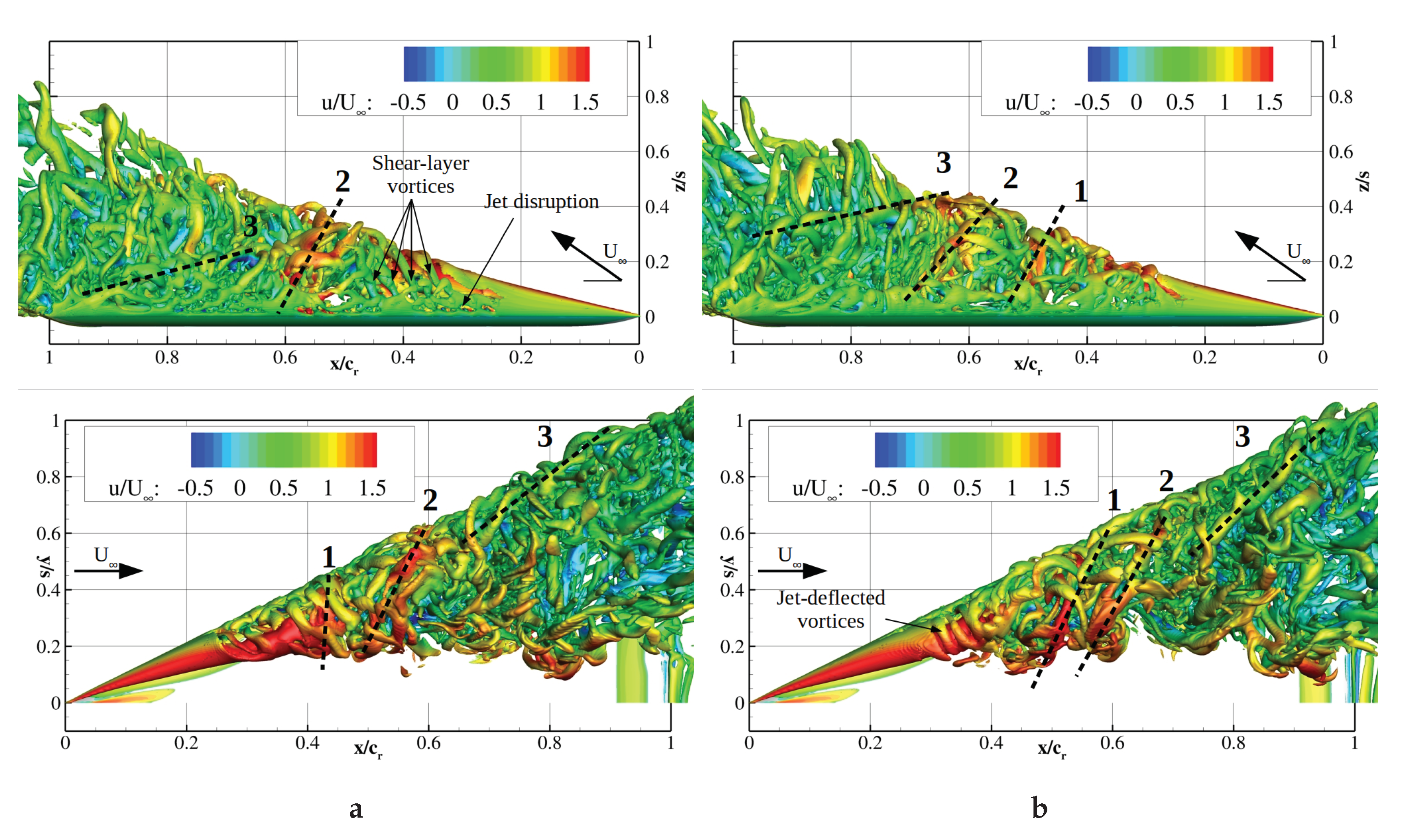
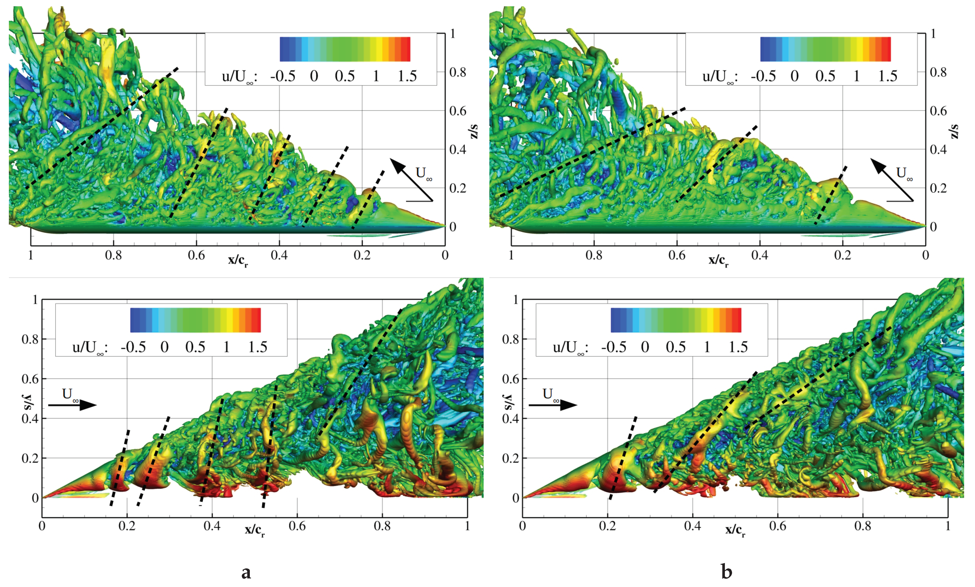
Computed Q-criterion isosurfaces ($Q={10}^{-5}$ s${}^{-2}$) of the equivalent corresponding time steps, during and $T/2$ after disturbance injection, are visualized in Figure 14. Hence, the phase averaged vorticity peaks in Figure 13 represented waves of local discrete vortices. Blowing excited merely the shear layer, but affected the whole vortex system with a time delay of $T/2$. In Figure 14a, shear layer vortices spiral around the steady core. Downstream, the waves of vortices designated by dashed lines wound up in the opposite direction compared to the shear layer vortices upstream of breakdown. The disruptions of the shear layer in Figure 14a were caused by the discrete jet being switched on/off. The flow field evolved $T/2$ after the formation of discrete jet vortices at the apex and downstream injected front of multiple vortices according to Figure 14b. At this particular time step, the numbered vortex clusters were located farther downstream with an increased tilting towards the freestream direction. In conclusion, synchronizing the jets at the leading-edge generated vortex clusters transporting high axial momentum $u/U_{\infty }>1.0$ towards the core in a periodic manner.

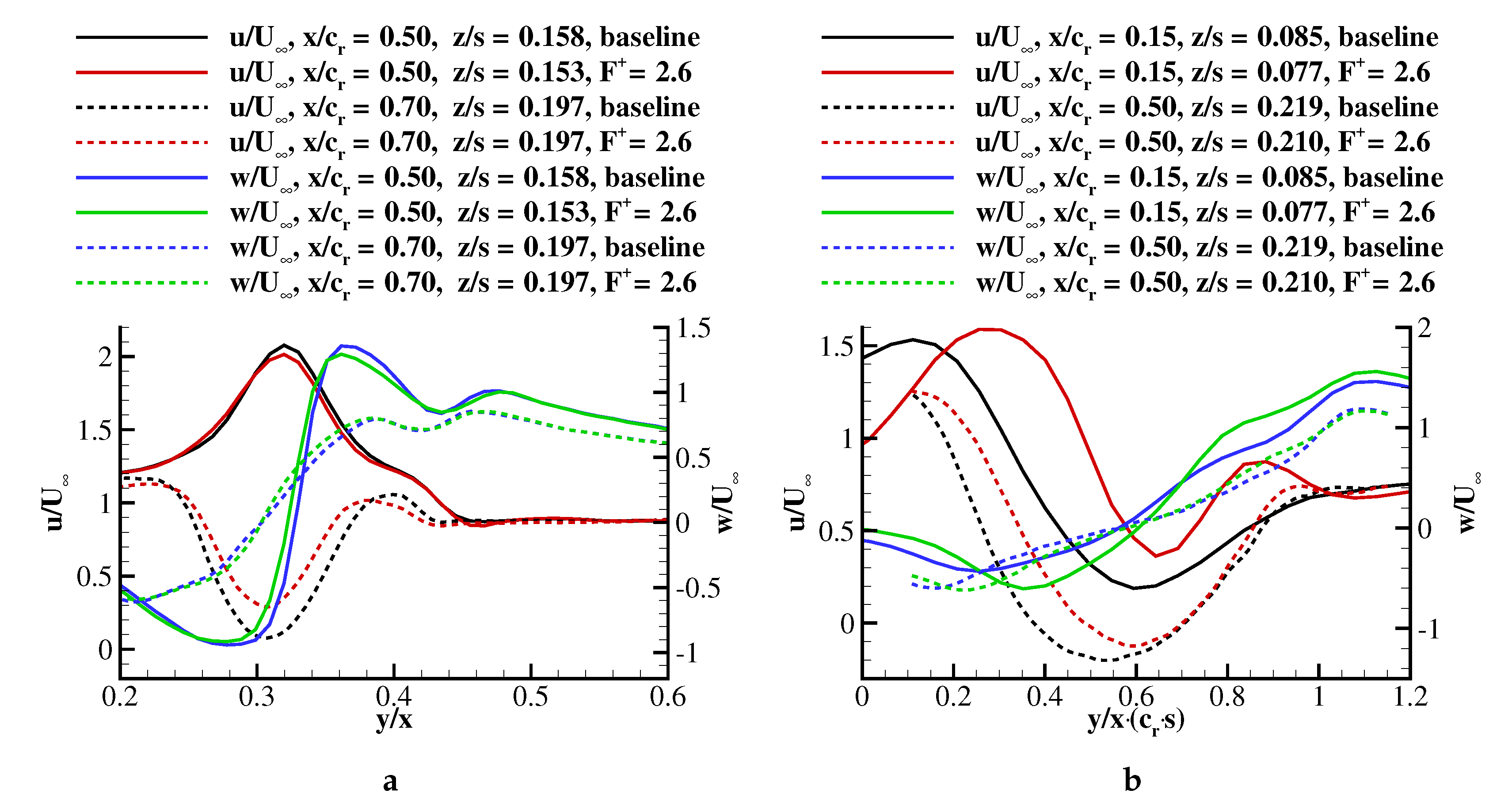
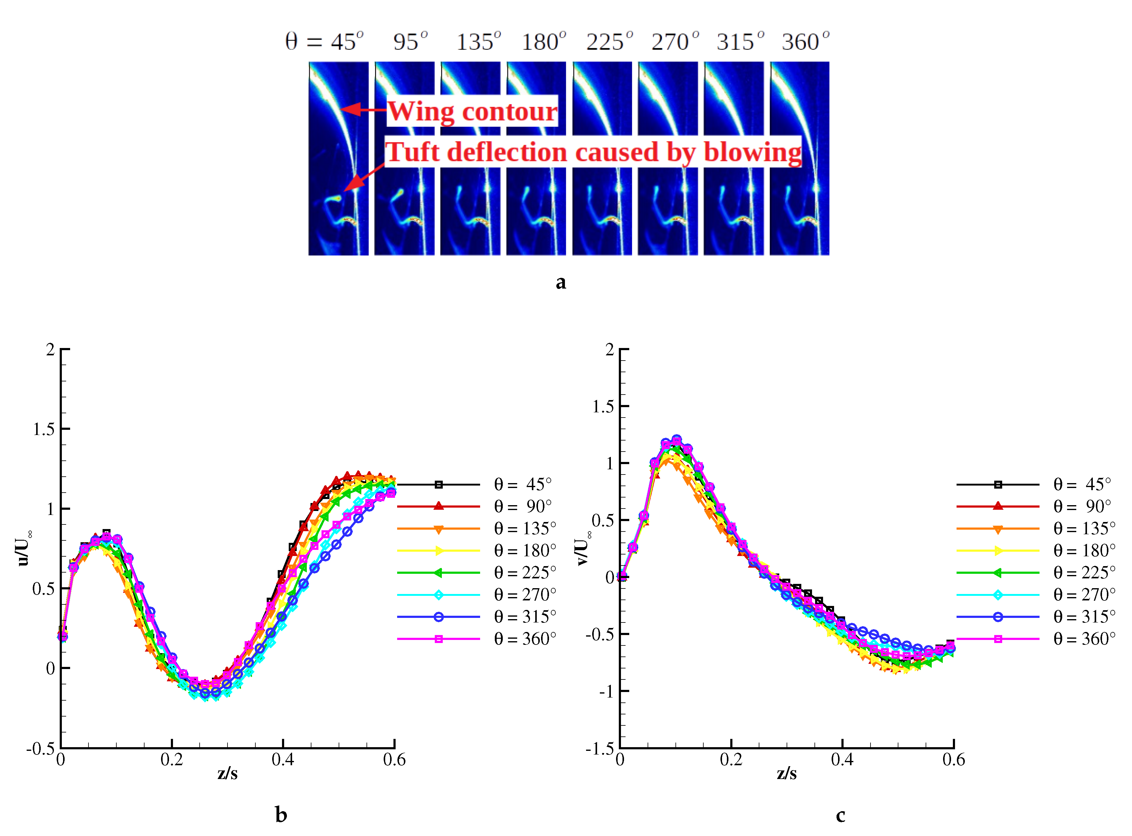
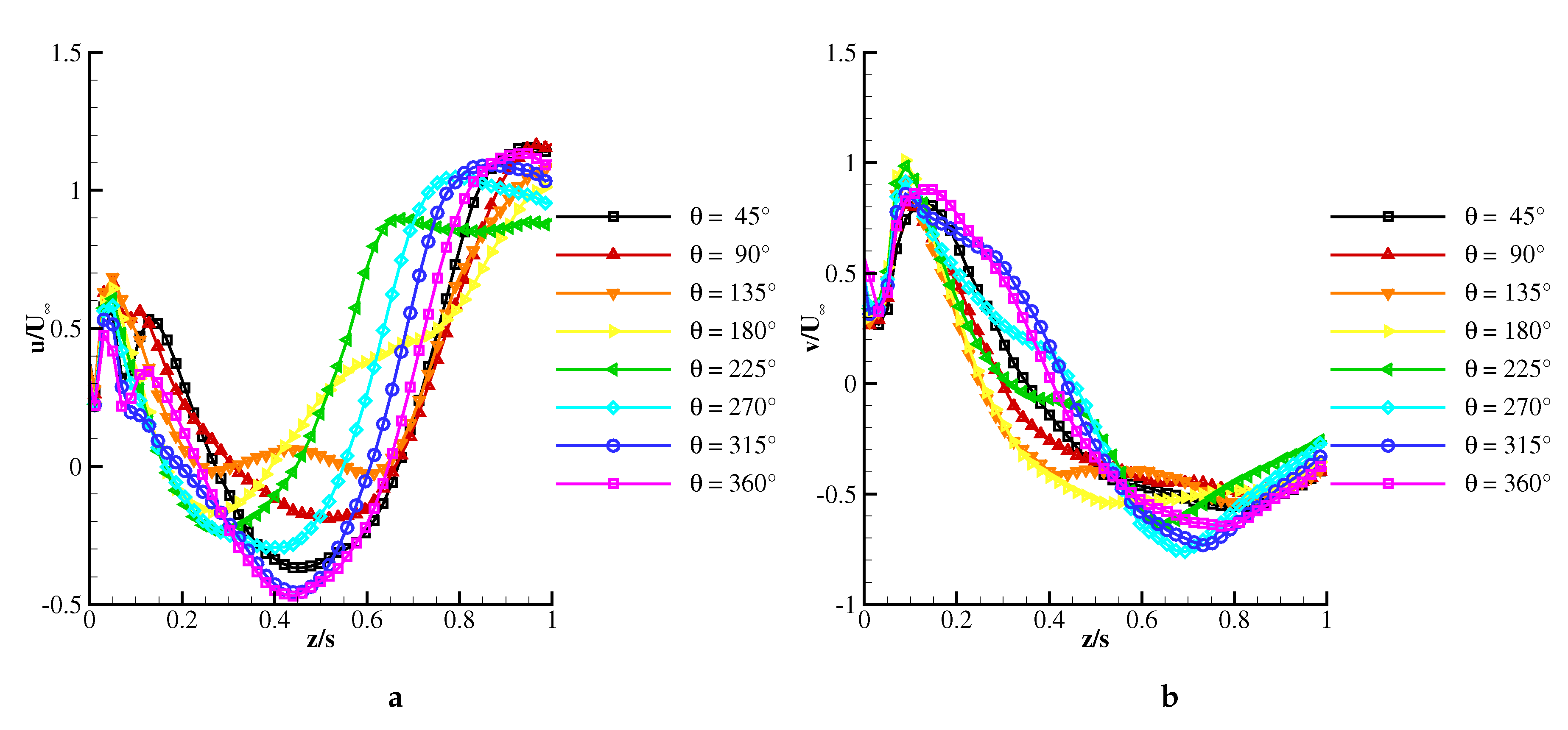
In order to investigate the transport of momentum, phase averaged vertical velocity profiles $u/U_{\infty }$ and $v/U_{\infty }$ were extracted from the crossflow plane at $x/c_r=0.65$ (above the first slot pair of the second segment) and plotted in Figure 15. The graphs represent eight equally distributed phases of one actuation period, in which the first 25% ($\theta =45°,90°$) of the period fluid was injected through the slots and the rest of the period, the jets were turned off. This is visualized by the deflection of a wool tuft placed above a slot in Figure 15a. The spanwise position of the extracted velocity profiles coincided with the mean vortex position of the actuated case. At $x/c_r=0.65$, the mean vortex axis was located at lateral and vertical positions relative to the half span of $y/s=0.36$ and $z/s=0.27$.

The near-wall region around $z/s=0.1$ was dominated by velocity components close to the freestream value: $u/U_{\infty }\approx 0.8$, $v/U_{\infty }\approx 1.1$. In the wake region farther from the wall, the axial velocity decreased, reaching a minimum of $u/U_{\infty }\approx -0.2$ in the vortex rotation axis. Both near-wall and wake regions fluctuated during the blowing period. There was a delay in the flow response to the actuation observed in the presented graphs. The near-wall velocity decreased with advancing phase. The velocity peaks closest to the wall had a minimum at the phase $\theta =135°$ for both components (cf. the orange graphs in Figure 15b,c). With progressing phase angle, the flow field recovered to the initial state with near-wall velocity components steadily increasing. Hence, the perturbation affected the flow field with a phase delay of approximately $T/4$ ($\Delta \theta =90°$).

Similarly, the wake region reacted to blowing by reducing axial velocity. The minimum value was reached at phases $\theta =225°$–$270°$, leading to a $T/2$ delay relative to the blowing phase. After the blowing phase $\theta =45°$, the wake cross-section increased steadily as suggested by the $u/U_{\infty }$ distribution above $z/s=0.4$. Here, the lowest axial velocities corresponded to the blue line, representing $\theta =315°$. Hence, the flow region above the wake responded to the actuation after a $3/4$ period. The distribution of lateral velocity presented in Figure 15c suggested a similar phase dependence as that of the axial velocity. The blue graph is situated above the other graphs both below and above the wake. The $v/U_{\infty }$ distribution described a distinct inflection in the first phase. Advancing in phase decreased the inflection.

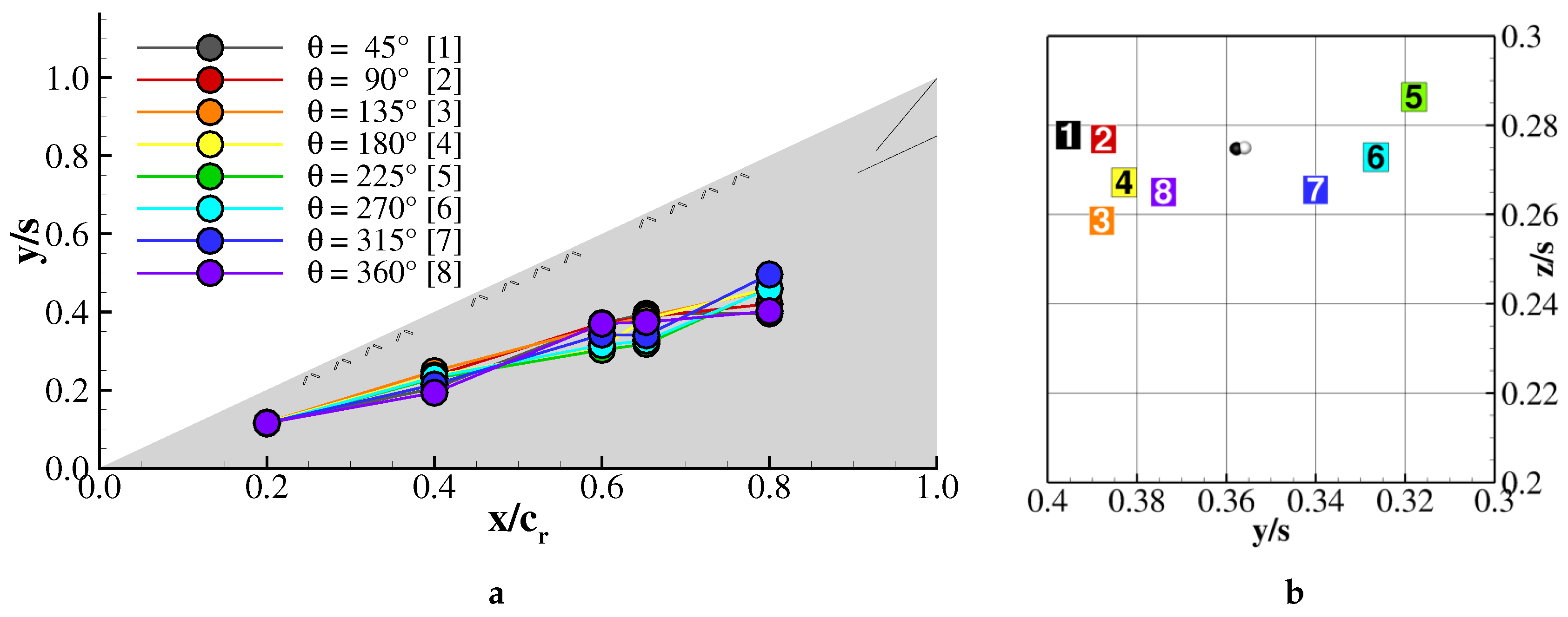
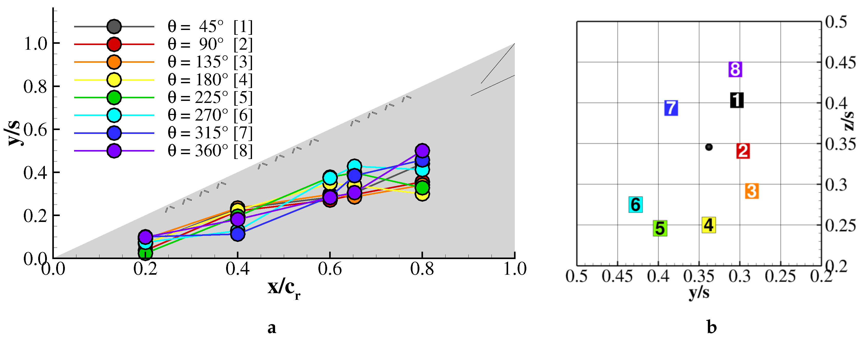
The above investigation into the flow field response based on phase averaged PIV measurements established a periodic displacement of the primary structure. The phase dependent location of the rotation axis is presented in Figure 16 from two perspectives, $xy$-plane (a) and cross-plane at $x/c_r=0.65$ (b). The vortex rotation axis described a slight curling around the mean axis. During periodic blowing, the axis displaced in a nearly elliptical manner. In the crossflow plane presented, the lateral motion was more pronounced than the vertical one. The largest displacement occurred in the first and fifth phases investigated. Hence, concomitant with the blowing, the vortex had the most outboard position at $y/s=0.4$ and remained in the vicinity up to the fourth phase ($\theta =180°$), after which, it moved to $y/s=0.3$. In addition to the phase averaged locations, Figure 16b displays in white the mean location of the baseline vortex axis and in black the one of the forced vortex axis. Although the vortex fluctuated and undulated under periodic forcing, its mean location was slightly outboards of the unforced vortex mean location. It should also be noted that the vortex pulsated at the forced frequency in the longitudinal direction.

3.4.2. Shear Layer Reattachment

In contrast to the stall case, in which pulsed blowing reduced the swirling wake, at $\alpha =45°$, the excitation targeted the shear layer reattachment that generated massive lift increase. The optimum reduced actuation frequency at this angle of attack was $F^{+}=1.0$, which was lower than the previous case. In [25], the power spectral density of the shear layer velocity fluctuations described a reduction of the dominant frequency when the flow was actuated, which suggested that manipulation of the shear layer instability reordered the shear layer vortices. This interaction resulted in the previously mentioned reattachment of the mixing layer on the wing’s surface. Figure 17 shows the phase averaged axial vorticity distribution at two phases of one blowing period. The phase on the left hand side corresponds to when the jets were switched off (Figure 17a). Immediately after blowing, the generated jets disrupted the shear layer, generating high vorticity concentrations above the leading-edge. The subsequent phases described the clockwise rotation of vorticity peaks. At a time delay of $T/4$, the vorticity peaks were displaced along the shear layer (Figure 17b).

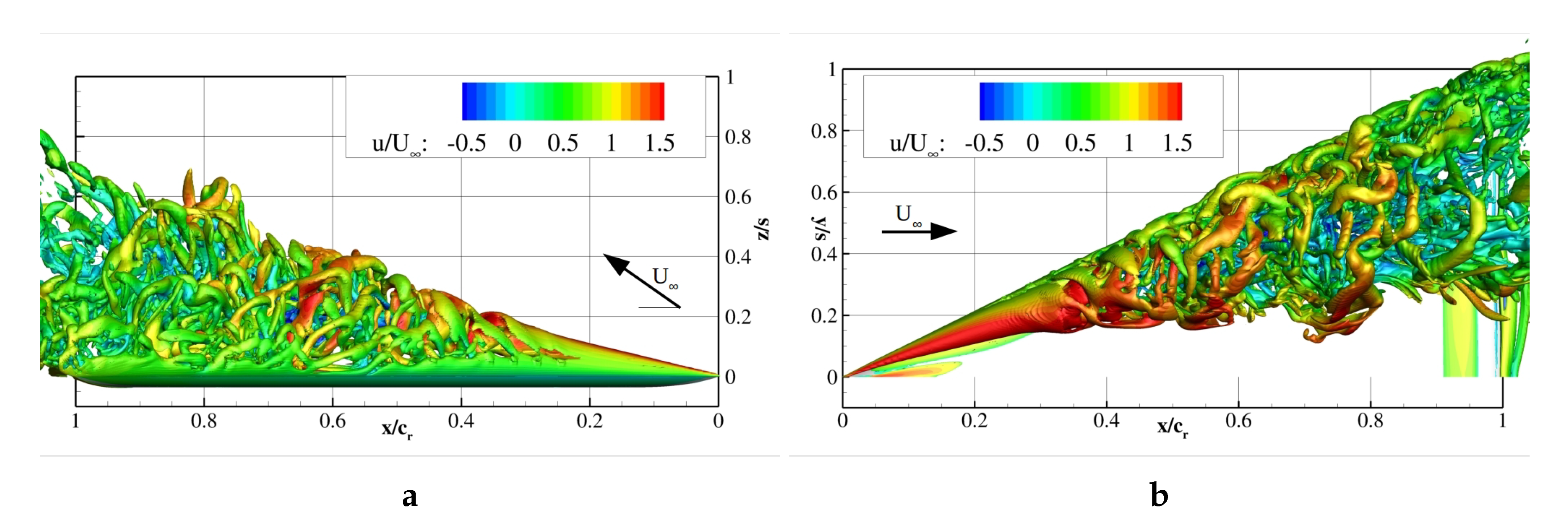
In Figure 18, the Q-criterion $Q={10}^5$ s${}^{-2}$ colored by the relative axial velocity in the range $-0.5\le u/U_{\infty }\le 1.5$ showed both investigated phases. The reattachment of the shear layer generated a flow field resembling the stalled flow field. At post-stall, the forced primary structure extended from the symmetry plane to the leading-edge. The pulsed jets increased the circumferential momentum, on the one hand, and enforced a frequency dependent vortex shedding, on the other. As a result, the shear layer consisted of unsteady discrete vortices rotating around the reversed flow region. The leading-edge shedding occurred in a three-dimensional manner as in the baseline case (cf. Figure 10). However, in the actuated case, the vortices were dominated by the jet interaction and increased in intensity downstream with specific curling around the wake. Dashed lines designate vortex fronts that demonstrated a certain periodicity. When the blowing ceases, the vortex fronts were ordered circumferentially and convected downstream; see Figure 18a. These waves originated from the shear layer instability initiated at the apex. Inboard, the flow constriction led to high axial velocities. $T/4$, after blowing cessation, waves of shear layer vortices nearly parallel to the leading-edge were present in the flow field, disturbing the annular structures. Advancing within the blowing period, the discrete vortices were transported downstream in a spiraling path, recovering to the initial state. Throughout this process, mixing between the inner wake region and the outer region was sustained.

Figure 19 presents the vertical distribution of $u/U_{\infty }$ and $v/U_{\infty }$ across the mean vortex core at $x/c_r=0.65$ and $y/s=0.34$. As in the previous case, jets were active during phases $\theta =45°-90°$ and inactive during the rest of the blowing period. In the region adjacent to the wall, axial and spanwise momentum increased steadily up to $\theta =180°$. As the phase progressed, both velocity components decreased, and the velocity deficit closer to the wing increased. Farther from the wall, the negative axial velocity peak fluctuated in a phase dependent manner. Axial velocity was at its lowest during the last quarter period, $\theta =315°-360°$. The blowing phase led to a rapid increase in axial velocity. The highest values corresponded to $\theta =135°$. At this phase, the wake-type distribution showed two valleys. The spanwise velocity component demonstrated an inflection, as well at 135$°$, which remained up to $315°$.

The fluctuation of the velocity field across the vortex described above suggested that the vortex underwent certain periodic motion within one blowing period. The location of the rotation axis corresponding to each phase investigated is plotted in Figure 20. As in the previous case, the vortex rotation center wound downstream in a counter-clockwise direction, but described a clockwise rotating path as time passed. At $x/c_r=0.65$, the phase averaged axis of rotation described an ellipse. During blowing, the axis had the most inboard displacement. Up to $\theta =135°$, the vortex axis shifted towards the wing, after which it described a lateral movement. Half a period after fluid injection, the vortex had the furthest outboard location. Comparing the phase averaged PIV investigations with the time accurate DES computations revealed that the primary structure consisted of many discrete structures that, on average, described an ordered motion.

4. Conclusions

This study focused on leading-edge vortex manipulation by pulsed blowing. First, state-of-the-art investigations into frequency modulated separated flows were presented. For separation control, optimum actuation frequencies at the minimum momentum coefficient were demonstrated to take values of $F^{+}=\mathcal{O}\left(1\right)$. In addition, the shear layer was more receptive to distortions injected in a 2D manner than in 3D one (phase delayed blowing). Therefore, current non-intrusive investigations (PIV and DES) on the baseline and synchronously excited leading-edge vortex flow at three high angles of attack, $\alpha =23°$, $35°$, and $45°$, were discussed.

At $\alpha =23°$, the leading-edge vortex broke down at approximately $x/c_r=0.6$, with a deviation of 10% between PIV and CFD, bearing in mind that the averaging times of the statistical quantities differed by one order of magnitude. While the angle of attack increased, the breakdown location moved upstream, reaching the apex region at $\alpha =35°$. This led to the vortex increasing in diameter, leading to stronger interaction with the shear layer. Both rms and instantaneous vector fields revealed increasing unsteadiness with the angle of attack. This was the product of amplified instabilities leading to the generation of discrete vortices. The post-stall flow field constituted a massive flow detachment over the entire wing. DES results revealed the typical vortex shedding and downstream convection without reattachment.

Periodic excitation on the vortex field by pulsed blowing altered the flow field, depending on the flight regime investigated. At $\alpha =23°$ and 35$°$, periodic blowing was tuned to the helical mode instability, $F^{+}=2.6$. The perturbations in the form of vortex waves were not induced in the stable vortex core and had little influence on it. However, strong interaction occurred with the wake region, displacing the breakdown location downstream. In conclusion, pulsed blowing at the leading-edge excited the shear layer, which convected the disturbance as vortex wave fronts around the breakdown wake, in a downstream clockwise winding path. The additional momentum and vorticity in the shear layer rolling around the low energy core reduced its cross-sectional area.

Massive lift increase was observed at $\alpha =45°$, where pulsed blowing reordered the leading-edge shedding mechanism, leading to stronger vortices that induced shear layer reattachment. Phase averaged PIV and time accurate DES results described the flow field evolution during one blowing period, starting with the $T/4$ blowing portion and ending with the recuperation phases. Waves of vortices wound counter-clockwise around the reversed flow core, but were convected downstream in a clockwise path. Synchronizing the jets at the leading-edge generated vortex waves with a more longitudinal orientation than in the baseline flow field, responsible for additional longitudinal vorticity.