Article

Modeling of High Density Polyethylene Regression Rate in the Simulation of Hybrid Rocket Flowfields

1
Department of Mechanical and Aerospace Engineering, Sapienza University of Rome, Via Eudossiana 18, 00184 Rome, Italy
2
Department of Industrial Engineering, University of Naples “Federico II”, Piazzale Tecchio 80, 80125 Naples, Italy
*
Author to whom correspondence should be addressed.
Aerospace 2019, 6(8), 88; https://doi.org/10.3390/aerospace6080088
Submission received: 21 April 2019 / Revised: 25 July 2019 / Accepted: 31 July 2019 / Published: 9 August 2019

Abstract

:
Numerical analysis of hybrid rocket internal ballistics is carried out with a Reynolds-averaged Navier–Stokes solver integrated with a customized gas–surface interaction wall boundary condition and coupled with a radiation code based on the discrete transfer method. The fuel grain wall boundary condition is based on species, mass, and energy conservation equations coupled with thermal radiation exchange and finite-rate kinetics for fuel pyrolysis modeling. Fuel pyrolysis is governed by the convective and radiative heat flux reaching the surface and by the energy required for the propellant grain to heat up and pyrolyze. Attention is focused here on a set of static firings performed with a lab-scale GOX/HDPE motor working at relatively low oxidizer mass fluxes. A sensitivity analysis was carried out on the literature pyrolysis models for HDPE, to evaluate the possible role of the uncertainty of such models on the actual prediction of the regression rate. A reasonable agreement between the measured and computed averaged regression rate and chamber pressure was obtained, with a noticeable improvement with respect to solutions without including radiative energy exchange.

1. Introduction

Hybrid Rocket Engines (HRE) are identified as promising propulsion systems for space transportation application [1,2]. Their performance is comparable to that of storable or semi-cryo liquid rocket engines, and they exhibit appealing features of both solid rocket motors and liquid rocket engines. Moreover, they are safer and less expensive than solid and liquid rockets and are more environmentally friendly than solid rockets and storable-liquid rockets. Therefore, many research programs have been focusing on HRE development for applications that range from Earth-suborbital flights to space exploration. Despite the above-mentioned advantages, some issues hinder the success of HRE: low regression rates of commonly used polymeric fuels, reduced combustion efficiency, mixture ratio shifts, the uncertainty of regression rate law, and its scalability are the most challenging problems. Uncertainty in the regression rate and its scalability remain some of the most challenging issues, since the regression rate is a parameter that strongly drives the design process and heavily influences the performance of the entire propulsion system.
To date, research efforts in developing reliable hybrid propulsion systems have strongly depended on firing tests and experimental trials and errors, which are expensive and time-consuming. In particular, as concerns the estimate of the fuel regression rate, empirical correlations based on linear interpolation in the logarithmic plane are mostly used, as well as surface energy balances, which include the simplified boundary layer correlations based on bulk transfer coefficients to evaluate the convective heat flux to the solid fuel. Such approaches are particularly useful during the preliminary design and analysis process, providing a simpler and faster estimation of the rocket performance, but they rely on a very simplified modeling of the mutually-interacting and complex physico-chemical phenomena involved. Therefore, they should be carefully calibrated relying on the availability of specific experimental data existing for each analyzed motor. Consequently, such models are limited to providing a qualitative analysis of the motor trends, but they are insufficient for providing the kind of quantitative data that are required for motor final design and optimization. Indeed, the extension of those models to new motors that can be different in geometry, scale, etc., is hardly possible without the availability of existing experimental data for each motor. For these reasons, there is a renewed interest in the development of more accurate and advanced models based on Computational Fluid Dynamics (CFD) [3,4,5,6,7,8,9,10,11,12,13,14,15] that are capable of representing more accurately the physico-chemical phenomena involved. The numerical modeling of the fluid dynamics and the combustion process in the fuel port area and nozzle of a hybrid rocket is a challenging task as it involves strongly-interacting multiphysics processes such as fluid dynamics, fuel pyrolysis [16,17], atomization and vaporization of the oxidizer, mixing and combustion in the gas phase [11,12,13,18], thermochemical erosion of the nozzle [3,19], particulate formation, and the radiative characteristics of the flame. Commercial CFD tools are generally not optimized to this task, as they are typically less flexible for the treatment of fluid/solid boundary conditions, which are typically prescribed as constant temperature or heat flux with no feedback with the mass transfer mechanisms (pyrolysis, sublimation, etc.). To obtain an adequate tool for the analysis of the flowfield of hybrid rocket burning classical non-liquefying fuels, CFD codes should take into account spatially-varying heat flux, surface temperature, and fuel regression rate, realistic surface multispecies mass and energy balances, thermal soak into the fuel grain, radiative energy exchange, and finite-rate Arrhenius kinetics for fuel pyrolysis modeling or, in the case of commercial solvers, a number of user-defined functions need to be built and integrated in the numerical framework [8,14,20]. In the most general case, an in-house code has to be used.
The goal of this study is the high-fidelity simulation of the internal ballistics of a hybrid rocket, including the pre- and post-combustion chamber and nozzle. The reference configuration was a 1-kN-class lab-scale hybrid rocket tested at the University of Naples “Federico II” and equipped with an axial subsonic injector nozzle that feeds gaseous oxygen into the port of High-Density Polyethylene (HDPE) grains. With such an injector arrangement, the regression rate results in being appreciably larger than what expected from the literature [21], in particular at the very low mass fluxes (around 10 kg/m 2 ·s) that exhibit a 2.4 -fold increase [18]; it also shows a lower dependence on the mass flux, and at a given mass flux, an increase with the port diameter is achieved. Furthermore, combustion efficiency and motor stability are both favored.
The numerical simulations presented here were carried out by solving the Reynolds-averaged Navier–Stokes equations for multicomponent, single-phase, turbulent reacting flows [22,23], including the sub-models required in order to describe the homogeneous combustion in the gaseous phase, the radiative energy exchange, and the gas–surface interaction in the combustion chamber (fuel pyrolysis model) for HDPE grains. The in-house computational tool used for the simulations, and its gas–surface interaction capability has been validated for high-speed re-entry flows [24], for the analysis of Hydroxyl-Terminated Polybutadiene (HTPB) fuel grains [3,4,25], and for hybrid rocket nozzle thermal protection systems’ ablation [3,19,26]. Recent literature works focusing on HDPE fuel grains in hybrid rockets either used commercial CFD tools with user-defined functions to compute the fuel mass flux as a function of the wall heat flux [8,14] or in-house CFD code [15] with imposed fuel mass flux using the mean regression rates measured during the firing test. Thermal radiation was not taken into account in [14,15]. Interestingly, the work in [8] showed that the regression rate was underestimated by 30% for high-density polyethylene grains when radiative heat exchange was not accounted for. The authors concluded stating that no clear information exists regarding the relative importance of radiative heat flux with respect to the convective one for HDPE grains at relatively low gaseous oxygen mass fluxes. The current work also aims at providing some insight into the effect of thermal radiation for HDPE regression rate predictions. Two main contributions to the field of hybrid rocket internal ballistics numerical simulation are addressed in this paper: First, a sensitivity analysis of the regression rate and chamber pressure to the pyrolysis models for HDPE available in the literature is carried out, highlighting the main effect of the heat of pyrolysis against the much lower influence of the pyrolysis kinetics parameters, leading to the conclusion that the former has a key role in the correct motor performance prediction. Second, an evaluation of the possible contribution of the radiative energy exchange between combustion gases and the solid fuel on the regression rate calculation, which is often neglected in simulations, is conducted with a novel approach, showing that radiation seems to play a significant role, especially with low oxidizer mass fluxes. This represents a first step towards a complete modeling of radiative contribution, which should also include emission from soot particles.

2. Theoretical and Numerical Model

The study of HRE flowfields requires a suitable modeling of the motor internal ballistics including both gas–surface interaction (fuel pyrolysis) and gas phase reactions’ (pyrolyzed fuel and oxidizer combustion) sub-models. Concerning the former aspect, a detailed gas–surface interaction sub-model based on surface mass and energy balances for fuel pyrolysis, including thermal radiation exchange and finite-rate Arrhenius kinetics, was coupled with a chemically-reacting three-dimensional CFD code and a gray/non-scattering two-dimensional axisymmetric radiation code.
The CFD tool is a finite-volume solver for three-dimensional compressible multicomponent turbulent reacting flows [22,23], with temperature-variable thermodynamic and transport properties. The thermodynamic properties of individual species were approximated by seventh-order polynomials of temperature, while the transport properties were approximated by fourth-order polynomials [27]. Mixture properties for viscosity and thermal conductivity were derived from Wilke’s mixing rule [28]. The species diffusion model was based on a single effective diffusion coefficient obtained assuming a constant Schmidt number. The Spalart–Allmaras one-equation turbulence model [29] was used to compute the turbulent viscosity. The turbulent thermal conductivity and the turbulent species diffusivity were computed from the turbulent viscosity, the specific heat at constant pressure, and the turbulent Prandtl and Schmidt number. The gas-phase chemistry was modeled assuming a zero-dimensional, perfectly-stirred reactor model. The numerical code solved the time-dependent conservation equations of species, mass, momentum, and energy for the chemical nonequilibrium flowfield by adopting a standard finite-volume Godunov-type formulation. It used multi-block structured meshes and was second-order accurate in space. An explicit Runge–Kutta integration scheme was adopted to advance in time the ordinary differential equation system, resulting from the time-discretization.
Radiation energy exchange from the hot combustion gases to the pyrolyzing fuel surface was accounted for through a separate code for generic axisymmetric gray/diffuse boundaries and inhomogeneous gray/non-scattering media, based on the Discrete Transfer Method (DTM) [30]. The equations of the problem under scrutiny were written in finite form by discretizing the solid angle, at each node, and the path length, for each ray. The discretized equations were then integrated by means of a summation over the whole path length along each ray, in order to evaluate the corresponding radiative intensity, and over the whole solid angle at each surface node location, to evaluate the associated radiative wall heat flux. Finally, the field and wall local state parameters needed by the radiation tool were retrieved from the CFD simulations, with which the DTM computations were coupled. A suitable geometric ray-tracing procedure was also implemented in the DTM radiation code.

2.1. Gas-Surface Interaction Model for Pyrolyzing Fuels

To complete the formulation of the theoretical model, suitable boundary conditions that describe the physics of the surface phenomena must be specified at the gas–surface interface (i.e., “wall”). Such wall boundary conditions that are applicable to pyrolyzing fuels (such as HDPE) are detailed in the following.
Assuming that no material is being removed in a condensed phase (either solid or liquid), then the general conservation equations at the gas–surface interface over a pyrolyzing fuel wall can be written as follows [31]. The overall surface mass balance is:
m ˙ b = ( ρ v ) w = ρ s r ˙
where m ˙ b is the overall mass flux of the injected fuel pyrolysis products per unit area of the wall surface, ρ and v are the mixture gas density at the wall and its normal-to-wall bulk velocity component, and finally, ρ s and r ˙ are the solid fuel density and its regression rate, respectively. The surface mass balance for each generic species is:
ρ D i m y i η + ω ˙ i = ( ρ v ) w y i i = 1 , 2 , , N
where D i m is the i th species-to-mixture effective diffusion coefficient, y i the gas phase mass fraction of the i th species at the wall, N the total number of species, ω ˙ i is the rate of production per unit surface area of gas-phase species i due to fuel pyrolysis, and η is the coordinate axis normal to the surface and oriented from the solid to gas. The overall surface energy balance is:
k T η + i = 1 N h i ρ D i m y i η + m ˙ b h s + q ˙ rad abs = m ˙ b h w + q ˙ cond s s + q ˙ rad em
where h w represents the enthalpy of the gas mixture at the wall, h i the enthalpy of the single gas species at the wall temperature, h s the enthalpy of the solid fuel grain at the wall temperature, k the gas mixture thermal conductivity, T the gas temperature, and q ˙ cond s s the solid conduction heat flux inside the fuel grain. Note that the term m ˙ b h s represents the energy flux entering the surface due to fuel grain regression. Finally, radiation emitted from the hot combustion products and absorbed by the fuel grain, as well as emitted radiation from the fuel surface were included in the surface energy balance, Equation (3). The terms q ˙ rad abs and q ˙ rad em represent the absorbed and emitted radiation from the fuel grain surface, respectively. The absorbed radiative heat flux, which is the radiative heat flux coming from the gas and absorbed by the wall, is:
q ˙ rad abs = α w q ˙ rad = ϵ w q ˙ rad
where q ˙ rad represents the incident radiative heat flux that is evaluated from the radiation model. Note that, according to Kirchhoff’s law, the wall absorptivity α w is equal to the wall emissivity ϵ w . The emitted radiative heat flux, which is the radiative heat flux emitted from the wall because of its temperature T w , can be expressed as:
q ˙ rad em = ϵ w σ T w 4
where σ is the Stefan–Boltzmann constant, σ = 5.67 × 10 8 Wm 2 · K 4 .
As concerns the energy transfer into the solid fuel, it was assumed that the heat conduction was dominant in the direction normal to the fuel surface. Although axial temperature gradients certainly existed along the fuel surface, they were generally small if compared with those in the radial direction due to the negligible temperature variation along the fuel surface. Hence they could be assumed to represent a second-order effect. In a local coordinate system that is moving with the receding fuel surface, the steady-state conduction term q ˙ cond s s can be expressed as:
q ˙ cond s s = k s T s η = ρ s r ˙ c s ( T w T s i ) = m ˙ b c s ( T w T s i )
where c s and k s indicate the fuel heat capacity per unit mass and the fuel thermal conductivity, respectively, and T w and T s i are the fuel grain wall temperature and initial temperature, respectively. It is worth noting that the steady-state conduction heat flux, Equation (6), is affected by the fuel specific heat, but not by its thermal conductivity, which only influences the in-depth fuel grain temperature profile. The steady-state assumption appears as a reasonable approximation as long as the thermal lag in the solid phase is sufficiently short, which actually occurs in the hybrid rocket operating conditions to be simulated, i.e., moderately high fuel regression rates and low fuel thermal diffusivity.
The surface energy balance equation can be recast using Equation (2), in order to emphasize the contributions due to convection from the gas phase, net radiation, pyrolysis surface reactions, and conduction into the solid fuel grain by recalling that, by the definition of the mixture enthalpy at the wall, h w = i = 1 N y i h i :
i = 1 N ω ˙ i h i m ˙ b h s k T η convection + i = 1 N ω ˙ i h i m ˙ b h s ϵ w ( q ˙ rad σ T w 4 ) net radiation = i = 1 N ω ˙ i h i m ˙ b h s i = 1 N ω ˙ i h i m ˙ b h s pyrolysis + i = 1 N ω ˙ i h i m ˙ b h s q ˙ cond s s solid conduction
The chemical heat flux due to pyrolysis surface reactions can be expressed as:
q ˙ chem = m ˙ b i = 1 N ω ˙ i m ˙ b h i h s = m ˙ b Δ h p
where the term between parentheses represents the heat absorbed by the pyrolysis surface reactions, and hence, it is the so-called heat of pyrolysis (more correctly, a heat of thermal degradation or depolymerization), Δ h p . Note that, upon substitution of Equations (6) and (8) into Equation (7), one obtains the final form of the surface energy balance:
k T η + ϵ w ( q ˙ rad σ T w 4 ) = q ˙ conv + q ˙ rad net = ρ s r ˙ Δ h p + c s ( T w T s i )
which, by defining h v = Δ h p + c s ( T w T s i ) as the effective heat of gasification of the solid fuel, coincides with the classical regression rate expression derived by Marxman and Gilbert [32]:
r ˙ = q ˙ conv + q ˙ rad net ρ s h v
which shows that the fuel regression rate is proportional to the incoming heat flux (convective plus radiative) and is inversely proportional to the fuel density and its effective heat of gasification.
At each time step, the gas–surface interface boundary condition iteratively solves the overall mass balance, Equation (1), the species mass balance, Equation (2), and the energy balance, Equation (7), in order to compute the mixture composition at the fuel surface, the injected pyrolysis mass flux, and the wall temperature of the fuel grain.

2.2. HDPE Pyrolysis Model

The rate of production per unit surface area of gas-phase species i, ω ˙ i , appearing in Equations (2) and (7), has to be estimated based on the fuel pyrolysis model. The kinetics and energetics of fuel thermal degradation can be investigated with various experimental techniques, such as thermogravimetry, typically under much lower heating rates than those of hybrid propulsion. In particular, these techniques have been applied to HDPE, a fuel often considered for application to lab-scale hybrid motors with simple perforations. Surface regression (often called linear pyrolysis) experiments have been performed by different authors [33,34,35,36] in order to measure the regression rate and the surface temperature of the fuel, as well as its heat of pyrolysis (or of degradation). Under the effect of an external heating source, the fuel grain is subjected to an abrupt temperature rise and, only very close to the surface, undergoes a thermal decomposition into gases [37]. The fuel grain thermal behavior is usually separated in two zones: the conduction zone, where heat is penetrating into the fuel, and the superficial degradation zone, where the fuel thermal degradation occurs. The latter is typically more than one order of magnitude smaller than the former. According to Lengelle [37], assuming a first-order reaction, the superficial degradation zone is described by the conservation of the non-degraded (virgin) material along the material thickness, x, as:
ρ s r ˙ d Y p d x = ρ s Y p A · exp ( E a / R T w )
where Y p is the mass fraction of the virgin polymer. The terms A and E a are the pre-exponential factor (in sec 1 ) and the activation energy (in kJ/mol) of the fuel pyrolysis law, respectively, and R is the universal gas constant. With the details of the complete explicit calculation given by Lengelle [34], the relation between fuel regression rate and surface temperature is obtained,
r ˙ = A · exp ( E a / R T w ) 1 E a / R T w a s R 2
with a s being the fuel thermal diffusivity and R being a non-dimensional regression rate of the form:
R 2 = 1 [ ln ( Y p w ) ( 1 T s i / T w + Δ h p / c s T w ) Δ h p / c s T w ]
Equation (12) expresses that as the regression rate increases, the surface temperature has to increase in order to accelerate the degradation process to allow for the complete decomposition of the material into gases. The term Y p w , i.e., the mass fraction of the virgin polymer at the fuel surface, was assumed to be 0.01 . Equation (12) can be expressed in the form:
r ˙ = A ^ · exp ( E a / 2 R T w )
with:
A ^ = R A a s E a / R T w
where the term A ^ is expressed in m/s and is varying with temperature. A simpler Arrhenius-type pyrolysis law of the form:
r ˙ = A ¯ · exp ( E a / 2 R T w )
is often used for correlating the regression rate with surface temperature [38,39], where the term A ¯ represents the Arrhenius pre-exponential constant obtained from curve fitting of experimental data. Arrhenius-type pyrolysis laws of the form of Equation (16) can be obtained for various fuel formulations by plotting the fuel regression rate (in millimeters per second) vs. the reciprocal surface temperature 1 / T w (in degrees Kelvin). Experimental sets of data generally follow the same trend and fit quite well to a single straight line on the semilog plot represented by the Arrhenius-type expression of the form of Equation (16) [40]. Note that Equation (16) is given in the form of the pyrolysis law based on bulk kinetics (Equation (14)) where the term E a / 2 represents the value of the activation energy of the Arrhenius-type data fit [40]. The values assumed for these coefficients are reported in Table 1, according to [34]. Note that, because of the large value of the activation energy E a (Table 1), relevant regression rate changes can be generated with minor changes of the fuel surface temperature.
In this work, as a single one-step irreversible Arrhenius-type equation was adopted to model r ˙ = m ˙ b / ρ s , it was assumed that the only pyrolysis product of HDPE was the monomer ethylene ( C 2 H 4 ).
Hence, according to [6], the species production rate per unit surface area, ω ˙ i , is equal to m ˙ b for the species C 2 H 4 , while it is equal to zero for all the remaining gaseous species. As concerns the heat of pyrolysis, it could be directly evaluated from Equation (8); nevertheless, since the assumption that the pyrolysis gas is only composed by the monomer ethylene is necessarily an approximation, here, the heat of pyrolysis was rather derived from the available experimental data. According to [34], a value of 2.72 MJ/kg was assumed for the heat of pyrolysis of HDPE. All the HDPE properties used for the simulations are listed in Table 2.
Note that, although ethylene was assumed to be the only pyrolysis product, the gaseous mixture at the fuel surface was not solely composed of C 2 H 4 , as the other gaseous species (i.e., oxygen and the combustion gases) can actually reach/leave the surface due to diffusion and convection induced by wall blowing, as shown in Equation (2). The gaseous mixture composition at the HDPE surface, in fact, can be determined by solving the species surface mass balance, Equation (2), coupled with the surface energy balance, Equation (7), to guarantee that the correct amount of gaseous fuel is injected into the flowfield from the grain surface.

2.3. Gas Phase Reactions

Finite-rate gas phase reactions were modeled using a global reaction mechanism, because detailed chemical kinetics mechanisms [41] would include several species and many reactions and would be, on the one hand, computationally intensive and, on the other hand, beyond the scope of the present study, whose major purpose is to focus on the gas–surface interaction and its coupling with the internal ballistics. Therefore, gas phase reactions were modeled using a simplified two-step global reaction mechanism. Within this mechanism, the first irreversible global reaction step involved C 2 H 4 , the fuel pyrolysis product, and molecular oxygen to form CO and H 2 O and was considered first-order in both the fuel and oxidizer. The second global step was reversible and accounted for the formation of CO 2 .
C 2 H 4 + 1.5 O 2 2 CO + H 2 O + H 2
CO + 0.5 O 2 CO 2
According to [5,42], the net reaction rates of these two global steps can be expressed as follows, where [·] indicates the species concentration:
w ˙ 1 = k f 1 [ C 2 H 4 ] [ O 2 ] w ˙ 2 = k f 2 [ CO ] [ H 2 O ] 0.5 [ O 2 ] 0.25 k b 2 [ CO 2 ] [ H 2 O ] 0.5 [ O 2 ] 0.25
The resulting rates of production and destruction of species i per unit volume, w ˙ i , were obtained from the net reaction rates, w ˙ j , and the reaction stoichiometry:
w ˙ C 2 H 4 = M C 2 H 4 w ˙ 1 w ˙ O 2 = M O 2 { 1.5 w ˙ 1 0.5 w ˙ 2 } w ˙ CO = M CO { 2 w ˙ 1 w ˙ 2 } w ˙ H 2 O = M H 2 O w ˙ 1 w ˙ H 2 = M H 2 w ˙ 1 w ˙ CO 2 = M CO 2 w ˙ 2
where M is the molar mass of the generic species indicated as the subscript. The forward and backward reaction rates, k f and k b , for the two reaction steps are expressed as Arrhenius functions in the usual form k = A k T n k exp ( E a , k / R T ) , where the values of the constants used in this work are tabulated in Table 3.
The first global step rate constants were taken from the work of [5], while the second step was taken from [42], which is a modified version of the reaction used in [5,6] to account for oxy-fuel combustion conditions.

2.4. Radiation Model

The radiation heat flux is usually recognized to play a role in determining the fuel regression rate, especially when burning either metalized or carbon black solid fuels. Furthermore, according to [39], in addition to convection, radiation from soot and variable fluid properties across the boundary layer can have significant effects on the regression rate, even with pure polymers. Radiation from the gas phase is, instead, typically considered smaller than convection and soot radiation. Despite soot radiation being generally considered more important than radiation from combustion products in the gaseous phase, soot radiation modeling still involved much more uncertainties than gas radiation modeling. For this reason, as a first step towards complete modeling of radiative heat flux for the present gas–surface interaction model, only the radiative contribution from hot gases was taken into account and discussed. Marxman and Gilbert [32] and Muzzy [43] proposed the first fuel regression model incorporating the effect of the radiative heat flux of the gas phase to the wall. By means of their boundary layer diffusion-controlled regression theory, they showed that a small radiation heat flux would not significantly affect the regression rate for the well-known convective heat transfer blockage due to the increased fuel blowing. As expected, the radiation contribution grows with the engine scale, i.e., with fuel port diameter. However, it has been established that the radiant heat flux is relatively more significant under low mass flux and low oxidizer-to-fuel ratio conditions. Here, a separate model for the calculation of the radiation heat flux from the gas phase is presented. The basic hypotheses adopted include gray/diffuse wall and gray/non-scattering medium. The gray/diffuse wall assumption was deemed acceptable since thermal radiation from the wall is not a major contribution. The gray/non-scattering medium assumption, on the other hand, allows us to reduce the computational time enormously, thanks to a spectrally-averaged treatment. It was also assumed that the radiation energy exchange did not affect the flowfield significantly [44,45], a hypothesis that is justified in view of the relatively small weight (1% at most for the analyzed test cases) of total power lost through heat transfer and the radiative one in particular, as compared to the thermal power generated within the thrust chamber. This assumption reasonably allows avoiding the calculation of the radiative heat flux at each cell volume in the flowfield and, hence, to neglect its contribution to the energy conservation equation. The radiative heat flux was therefore only evaluated at selected nodes on the wall boundary.
The incident radiative wall heat flux, q ˙ rad , reaching a specific wall location and coming from other wall locations through the gas and from the gas, is defined by the following integral expression of the radiative intensity at the wall, I w , over the hemispherical solid angle that is facing the incoming radiation, Ω :
q ˙ rad = 2 π I w sin θ d Ω = 0 2 π 0 π 2 I w sin θ cos θ d θ d ψ
The radiative intensity at the wall from each generic line-of-sight can be computed by integrating the Radiative Transfer Equation (RTE) along the entire radiation path length. The RTE represents the balance of the radiative intensity along a generic direction, including contributions due to emission/absorption and, potentially, in-/out-scattering. Under the hypothesis of gray/non-scattering medium, it reduces to the form:
d I d s = j e κ I = κ I b κ I
where j e is the power emitted from the gas per unit volume, which can be expressed as proportional to black-body radiative intensity I b = σ T 4 / π through a proportionality constant for emission, which is the same as the absorption coefficient κ .
The RTE formal solution is then given by:
I w = I w , 0 exp s 0 s w κ d s + s 0 s w j e exp s s w κ d s d s
where it was assumed that the line-of-sight is originating from another wall point. The radiative intensity I w reaching a generic wall point from a given line-of-sight was hence due to the contributions I w , 0 from the origin of the line-of-sight and j e from each point in the medium along the line-of-sight. The exponential terms account for the radiation absorption by the medium from the origin (first term in Equation (21)) and through the medium itself (second term in Equation (21)). Equations (19) and (21) require the knowledge of the radiative intensity at the origin, I w , 0 , and of the absorption coefficient, κ , in order to be solved.
The radiative intensity at the origin, under the hypothesis of a gray/diffuse wall, is evaluated as:
I w , 0 = ϵ w , 0 σ T w , 0 4 + r w , 0 q ˙ rad , 0 π
taking into account both the radiative intensity that is emitted and reflected by the wall at the line-of-sight origin, where surface emissivity and reflectivity are ϵ w , 0 and r w , 0 , respectively. Assuming the wall as opaque, the radiation balance yields the relation r w + α w = 1 between reflectivity and absorptivity. Since such a boundary condition also depends on the radiative heat flux reflected by the wall, which in turn depends on the incoming radiative heat flux, q ˙ rad , 0 , an iterative procedure is hence required for the more general case of gray reflecting walls.
The absorption coefficient of the gas mixture was derived by means of a global model, which is typically used for high-temperature combustion gas mixtures under vibrational equilibrium conditions,
κ = p i = 1 N rad X i κ p , i
indicating that the absorption coefficient of radiative energy is proportional to the pressure, p, and to the absorption coefficients of the N rad participating species, weighted with their molar fraction, X i . In particular, water vapor, carbon monoxide, and carbon dioxide [46,47] are the most relevant species in the process of thermal radiation exchange. The present absorption coefficients, also known as Planck-mean absorption coefficients, were averaged over the whole wavelength spectrum. Their temperature dependence was given up to 5000 K and at atmospheric pressure in [48], by fitting and extending the curves reported in [46,47]. This model is adopted here, although not explicitly accounting for high-pressure effects, admittedly leaving some uncertainty, which is deemed of a weight comparable to those implied by other aspects of the model.
In the present work, the RTE was integrated by DTM using an in-house software for generic inhomogeneous gray/non-scattering media and axisymmetric gray/diffuse boundaries. The software was suitably developed and validated in [49,50].

3. Motor Configuration and Firing Tests

A basic description of the lab-scale motor and of the test facility that was employed to carry out the firing tests referred to in this work is reported here; more exhaustive data can be found in [51].
The lab-scale rocket had an axisymmetric combustion chamber; the main dimensions needed in the numerical simulations are reported in Figure 1 for the sake of the reader’s convenience. Several static firings were performed with this motor configuration using HDPE grains. All the experimental firing test data used in this paper were obtained with an axial injector configuration that employs a subsonic converging conical nozzle whose exit diameter was 8 mm. A stainless steel pre-chamber and a thermally insulated aft-mixing chamber were arranged upstream and downstream of the fuel grain, respectively. Gaseous oxygen was supplied to the motor feeding line through a pressure regulator and was measured by means of a calibrated Venturi tube. A water-cooled conical converging-diverging nozzle made of copper alloy with a 2.4 expansion ratio and a 16 mm throat diameter ensured long-duration firings without throat erosion. Chamber pressure was measured by using two capacitive transducers arranged in the pre-chamber and in the aft-mixing chamber.
Cylindrical HDPE grains with a single circular port were employed with a fixed length, and four different initial inner diameters (16, 25, 50, and 75 mm) were used to achieve a wide range of grain length to diameter ratios and of average mass fluxes at a limited expense of oxidizer mass flow rate (the maximum achievable oxygen flow rate being 350 g/s). The selected experimental test cases that were used for model sensitivity analysis and validation in this work are summarized in Table 4, which indicates the average parameters measured over the different firing tests. More details can be found in [51]. The firing test parameters were derived as follows.
The time- and space-averaged fuel regression rate was calculated via the fuel-mass loss method:
r ˙ ¯ = m ˙ ¯ f ρ s π D ¯ L
where m ˙ ¯ f represents the time-averaged fuel mass flow rate that is obtained by dividing the measured fuel mass loss, Δ M , by the burning time, t b :
m ˙ ¯ f = Δ M t b
The time-averaged (over the entire burning) port diameter, D ¯ = ( D 0 + D ^ 2 ) / 2 , was computed from the initial port diameter, D 0 , and the space-averaged final one, D ^ 2 . D ^ 2 was determined by means of the consumed fuel mass as follows:
D ^ 2 = D 0 2 + 4 Δ M π ρ s L
The determination of the burning time, t b , derived from the pressure-time trace, following a well-assessed procedure [51].
Finally, the time- and space-averaged mass flux was computed based on the average port diameter and the time-averaged mass flow rate (either the oxidizer or the total one):
G ¯ = 4 π m ˙ ¯ D ¯ 2
This averaging definition was demonstrated to be the most accurate and reliable in describing the classical power law of the regression rate over mass flux [52].

4. Domain Discretization and Boundary Conditions

In order to simulate the motor operating conditions and predict the internal ballistics in terms of motor regression rate and chamber pressure that were experimentally measured, the flow domain was discretized into a grid. The computational domain analyzed represented a simplified geometrical representation of the physical domain in which the pre-chamber, the fuel grain, and the post-chamber were all schematized with a constant cross-section (see Figure 2). Based on the available experimental data, the inflow boundary condition enforced the oxidizer static temperature and mass flow rate. More specifically, a single value for the oxygen inflow temperature ( T = 300 K) was imposed in all simulations, whereas different values for the oxygen mass flow rate were enforced according to the firing test (see Table 4). It is worth noting that the oxidizer mass flow rate was controlled by the choked Venturi injector and was held constant during the firing, regardless of the grain diameter and chamber pressure variations over time. The pyrolysis gas that was injected from the fuel wall was C 2 H 4 , and its amount was determined first by iteratively solving Equation (7) for the wall temperature and, then, by updating the gaseous chemical composition at the grain surface through Equations (2) and (16). Incoming net radiative heat flux was computed from the DTM radiation code as a post-processing of the CFD solution. The CFD code and radiation code were coupled until convergence was reached. Some iterations between the two codes were required to reach convergence as the radiation computed by the DTM code affected the fuel regression rate, which, in turn, affected the CFD solution. All the simulation presented here were axisymmetric and at the steady-state condition reached by iterating in time until the residuals dropped by five orders of magnitude. For each value of enforced inflow oxygen mass flow rate, the CFD solution provided a prediction of the fuel regression rate axial distribution (from the surface balances), as well as of the chamber pressure value in the motor arising from the choked condition at the nozzle throat. Hence, the chamber pressure level attained in the chamber depended on both the fuel mass flow rate and the mixing and combustion process.
Figure 2 shows the numerical grid for Firing Test #10 (see Table 4) at the average port diameter condition. An enlargement of the injection region is also shown that highlights the adopted grid refinement needed to capture the strong recirculation region induced by the axial injector. The computational domain was divided into 170 × 60 grid volumes in the axial and radial directions, respectively. Volume cells were clustered towards the surface so as to ensure a value of y + of about one at the wall-adjacent cell to accurately describe the boundary layer up to the wall all along the motor length. The dimension of the wall-adjacent cell at the fuel surface was of the order of 10 μ m. Additional axial clustering of cell volumes was placed in the region near the grain leading and trailing edges, as well as in the nozzle region. In the numerical simulations, the details of the leading- and trailing-edge regions of the fuel and the corresponding pre- and post-chamber cavities were omitted. Those simplifications of the actual geometrical details (Figure 1) allowed a reasonable computational time and accuracy in order to perform parametric analyses. A grid sensitivity analysis and a grid convergence analysis was carried out to ensure that the results were grid independent and to assess that the grid size and refinement was sufficient to obtain an accurate solution, respectively. A finer 340 × 120 mesh, made by doubling the grid volumes in both axial and radial directions with respect to the reference one, was also used for Firing Test #10. Results computed by the two grids showed a difference in the average chamber pressure and in the average regression rate of approximately 1% and 2%, respectively. Hence, the reference 170 × 60 grid was considered sufficiently refined for the present analysis.

5. Results and Discussion

For each experimental firing, which was characterized by a given oxygen mass flow rate (constant over the firing) and by an evolving port diameter due to the fuel regression, a single computation was performed at the average port diameter (known from measurements and reported in Table 4) and enforcing the experimentally-determined oxygen mass flow rate. Performing a single numerical simulation for each experimental firing is indeed a simplification of the actual test condition as the port diameter inevitably changes during the burning time. However, previous results [4] have shown that the time- and space-averaged regression rate computed through several computations performed at different grain geometries (each corresponding to a specific phase of the burn) only deviates by a few percent from the space-averaged regression rate derived from a single simulation computed at the average port diameter. Hence we assumed, here and in the following, that the space-averaged values computed from the simulations carried out at the average port diameter were representative of time- and spatially-averaged values measured in the tests. Moreover, the oxidizer mass flux and the port diameter of each simulation, respectively indicated with G ¯ o x and D ¯ , were to be considered as averaged values. As an example, Figure 3 shows the resulting temperature field at the average port diameter of Firing Test #19 with an oxygen mass flow rate of 94.5 g/s. The simulation showed that the flowfield in the motor entrance region was dominated by a strong recirculation region generated by the oxidizer axial injection. This hot recirculation region was instrumental in enhancing fuel and oxidizer mixing and combustion. Figure 3 also shows the cold region (<1000 K) close to the motor axis in the proximity of the axial oxygen injector.
Before comparing the computed results in terms of predicted fuel regression rate and motor chamber pressure with respect to the experimental measurements, a thorough sensitivity analysis of the fuel pyrolysis model was performed.

5.1. Sensitivity Analysis of the Pyrolysis Model

In order to understand how the law of pyrolysis and the heat of pyrolysis used in the surface energy balance can affect the regression rate and chamber pressure prediction, a sensitivity analysis was performed. In fact, aside from the reference model presented in Section 2.2 (see Table 1), other pyrolysis models are available in the literature. Hence, before comparing the obtained predictions with the experimental measurements, it was important to quantify the effect of the fuel pyrolysis model uncertainties on such predictions. For such a study, Firing Test #19 was taken as the reference because of its intermediate port diameter ( 47.19 mm) and oxidizer mass flux ( 54.03 kg/m 2 ·s) with respect to the operating conditions of the considered firing tests (Table 4).
The laws of pyrolysis available in the literature are widely scattered because of significantly different pre-exponential constants and activation energies. At a given temperature, this leads to significantly different values of regression rate, as is shown in Figure 4, where five different laws of pyrolysis are compared for HDPE fuel grain temperatures ranging approximately from 750 to 950 K. The five analyzed laws of pyrolysis were taken from different references in the open literature, and they were expressed either in the form of Equation (14) or in the form of Equation (16). In fact, when the pyrolysis reaction rates were obtained from thermogravimetric analyses, they were expressed in terms of reaction speeds with a pre-exponential factor A in sec 1 , while the pre-exponential constant A ¯ of Equation (16) was expressed in m/s and was obtained from curve fitting of surface regression experiments. When the form of Equation (14) was used, a pre-exponential term A ^ , which varied with temperature, could be computed from the pre-exponential factor, the fuel thermal diffusivity, and the non-dimensional regression rate from Equation (15).
Table 5 and Table 6 list the activation energy and the pre-exponential constant (see Table 5) or the pre-exponential factor (see Table 6) for the different HDPE pyrolysis laws. As shown in Figure 4, a significant scattering was evidenced between the various laws. Note that the r5 pyrolysis law, according to its authors [36], was obtained with a very low heating rate of about 20 K/min that was several orders of magnitude lower than the heating rate of the fuel in actual hybrid rocket combustion chamber conditions, which was estimated to be around 10 5 K/s [36]. For this reason, the r5 pyrolysis law was discarded from this analysis. The behavior of the r1, r2, and r3 laws showed a very similar slope (Figure 4) due to the fact that the activation energies were practically the same. Differently, the r4 pyrolysis law showed a significantly higher activation energy. Finally, although the regression rate of the r1, r2, r3, and r4 pyrolysis laws were comparable, they could show differences in r ˙ at the same temperature up to 40%. Therefore, it was of importance to analyze the effect of different activation energies and pre-exponential constants on the regression rate prediction in actual hybrid rocket conditions.
Starting from the reference law of pyrolysis r1 (blue curve in Figure 4), the following parameters were changed: first, the pre-exponential constant was modified by using the corresponding (lower) value from the law r2 (green curve in Figure 4), and second, the activation energy was modified by using the corresponding (higher) value from the law r4 (cyan curve in Figure 4). This was in order to analyze separately the effect of a change in each of the parameters A and E a of the pyrolysis law.

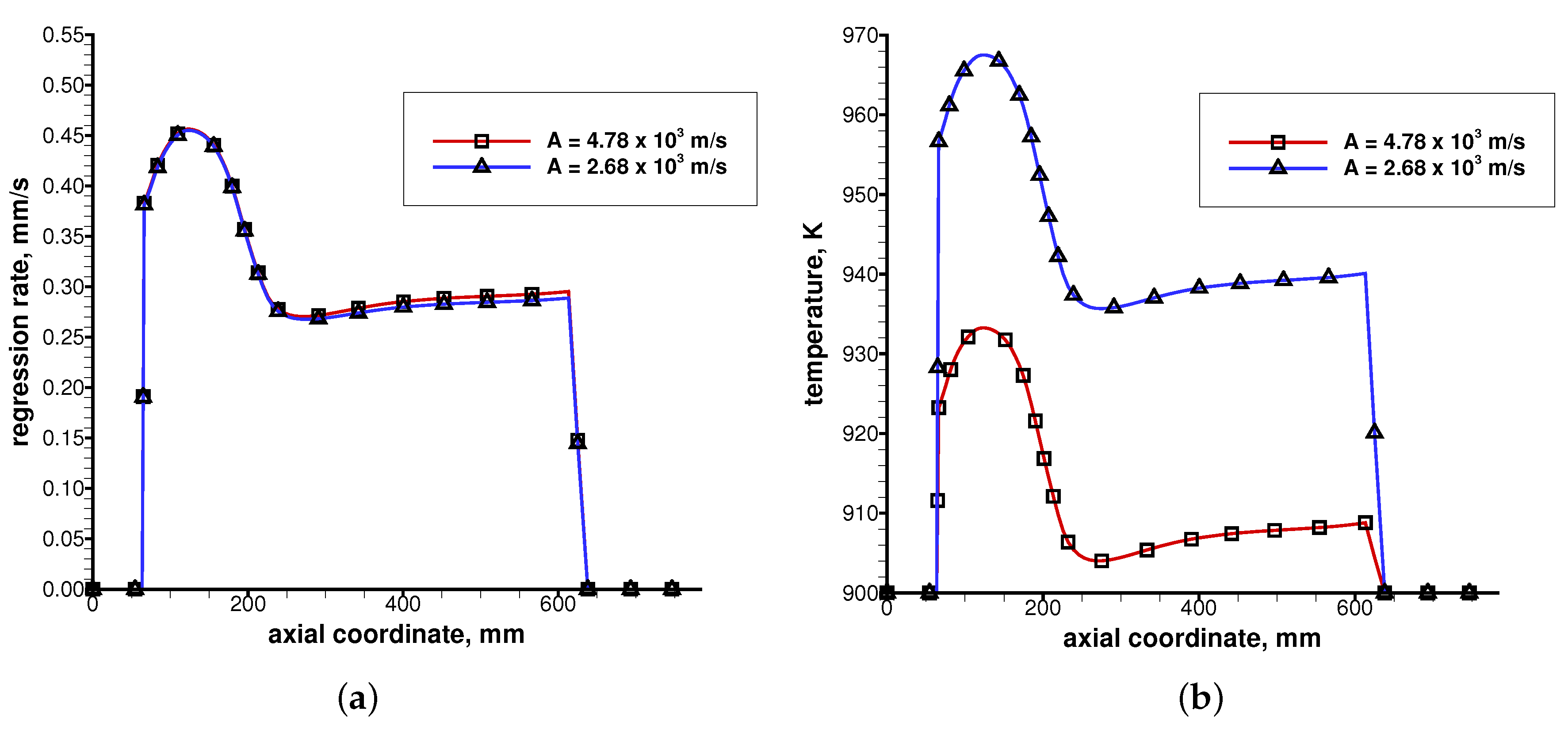
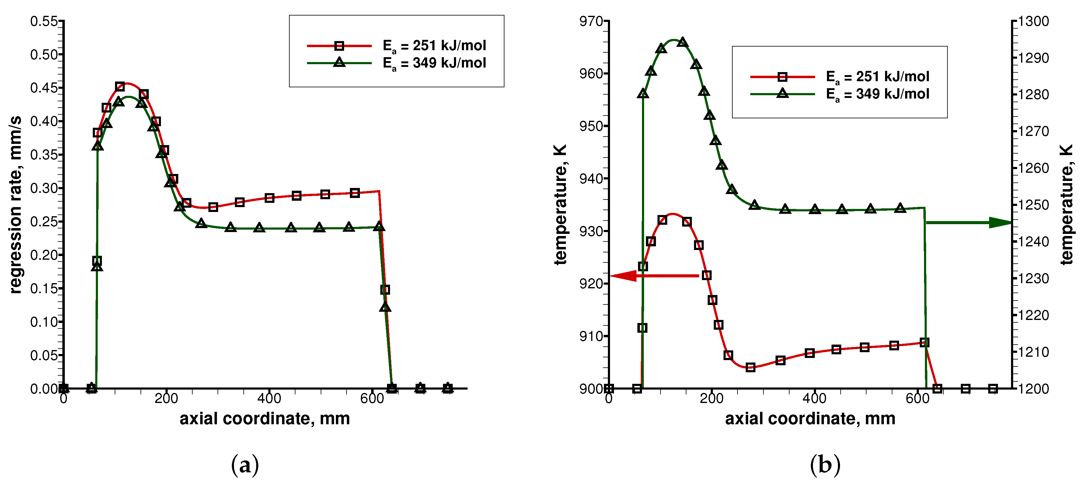
5.1.1. Sensitivity to the Pyrolysis Law Parameters

Figure 5 shows the effect of a 44% reduction in the pre-exponential constant (from 4.78 × 10 3 to 2.68 × 10 3 m/s) on both the fuel regression rate and the fuel temperature. Table 7 shows the results in terms of the space-averaged regression rate and motor chamber pressure.
Not surprisingly, once the widely-different pre-exponential constants were used in the gas–surface interaction wall boundary condition, very similar values of fuel regression rate were found, with a difference of the order of 1%. This was due to the fact that the wall temperature behaved as a compensating factor, while the regression rate was dominantly dictated by the incoming heat flux, Equation (10). In fact, when a lower pre-exponential constant was used, a higher wall temperature resulted from the energy balance (see Figure 5b), leading to a computed regression rate that remained practically unaffected (see Figure 5a). Thus, the pyrolysis process was certainly controlled by the heating of the fuel surface, with reaction kinetics only playing a minor role [32]. Hence, as shown in Figure 5 and in Table 7, the reduction in the pre-exponential constant of the pyrolysis law was almost completely compensated by the increased grain wall temperature (of the order of 30–40 K), leading to negligibly small variations of both regression rate and motor chamber pressure.
Figure 6 shows the effect of a 39% increase in the activation energy (from 251.04 to 349.00 kJ/mol) on both the fuel regression rate and the fuel temperature. Table 8 shows the results in terms of space-averaged regression rate and motor chamber pressure.
The effect of the increase of the activation energy was qualitatively similar to the effect of a decrease in the pre-exponential constant, although quantitative results were significantly different. As shown in Figure 6 and in Table 8, the increase in the activation energy was only partially compensated by the increased grain wall temperature, causing limited, but non-negligible variations of both the regression rate and chamber pressure. Although the analyzed percentage variations in the pre-exponential constant and activation energy were similar (44% and 39%, respectively), the effect of the activation energy on the overall results was much stronger than that of the pre-exponential constant, due to its exponential effect on the pyrolysis law. It must be stressed that the grain temperature increase was also much higher (of the order of 300–350 K) than in the previous case, thus causing a more significant reduction of the convective heat flux that translated into a regression rate reduction. Finally, it has to be noted that the present sensitivity analysis was carried out for the sake of investigation to understand the specific role of the two parameters (A and E a ) of the pyrolysis law. However, pyrolysis laws should be obviously used taking all the relevant parameters from a single reference, avoiding mismatches between parameters taken from different data. Therefore, a direct comparison between r1 and r4 pyrolysis laws will be later presented. We conclude this sensitivity analysis highlighting the fact that both the pre-exponential constant and the activation energy had a direct effect on the grain wall temperature, while they were only mildly affecting the grain regression rate and, hence, the motor chamber pressure. This was especially true for the pre-exponential constant.

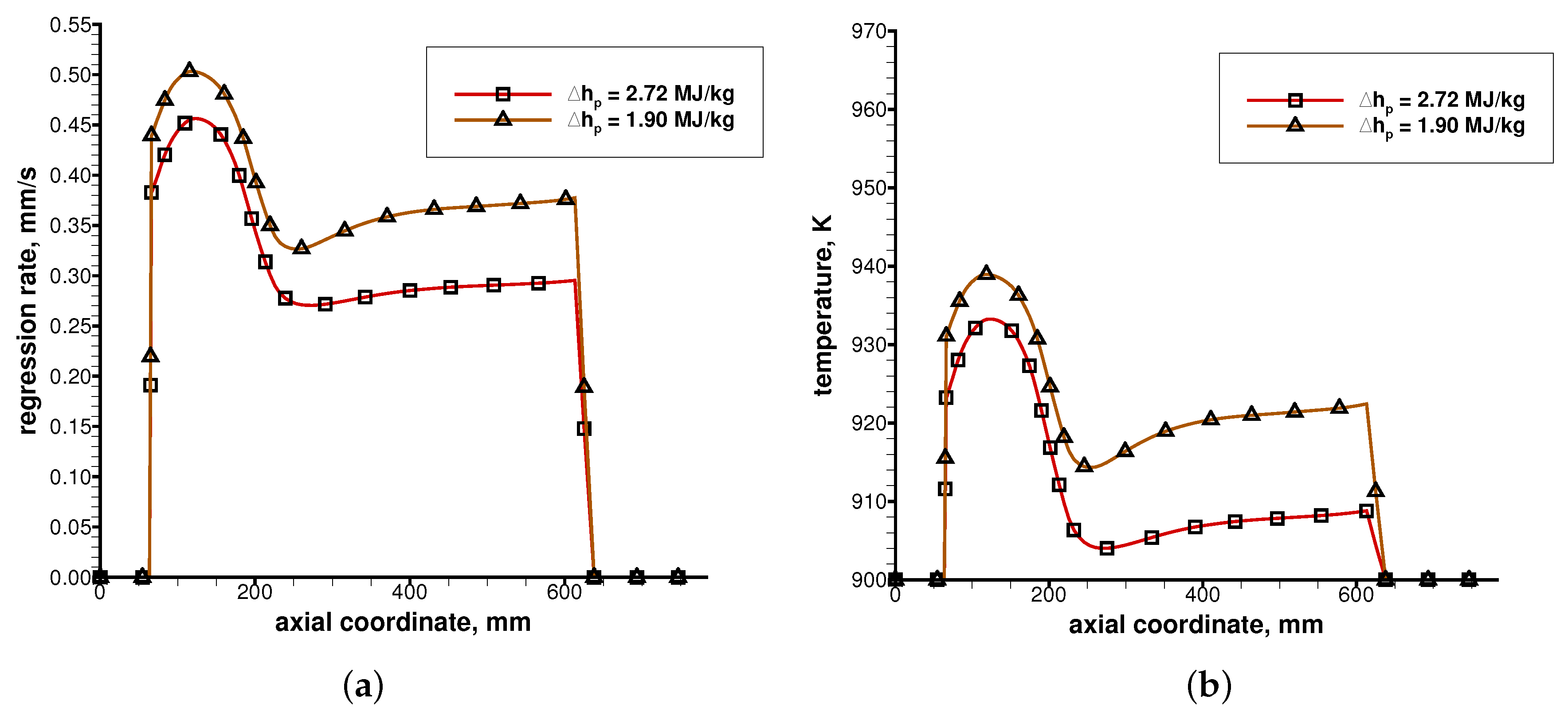
5.1.2. Sensitivity to the Heat of Pyrolysis

The last sensitivity that was analyzed, before comparing directly one complete set of pyrolysis law data to another complete set (r1 vs. r4), was the effect of the heat of pyrolysis, Δ h p . A significant scattering was found in the literature also for the heat of pyrolysis of HDPE. For such a reason, the heat of pyrolysis was reduced by an arbitrary amount of 30% with respect to the reference value ( 2.72 MJ/kg), listed in Table 2, in order to measure the direct effect of its change on the results in terms of regression rate and chamber pressure. The results presented in Figure 7 and Table 9 showed a strong sensitivity to the value assumed for the heat of pyrolysis. A modest rise of the grain wall temperature (of the order of 6–12 K) was also found because of the increased available energy associated with the lower heat of pyrolysis. However, different from the two previous cases (#19a and #19b), the effect of the heat of pyrolysis on the grain wall temperature was minimal (of the order of 1%), while the effect on the fuel regression rate (and hence, on the chamber pressure) was definitely more pronounced (+21% on the regression rate).
This, again, confirmed that the regression rate was dictated by the energy balance at the grain surface and by the competition between incoming heat fluxes (convection and radiation) and outgoing heat fluxes (fuel pyrolysis and solid grain heating), as shown in Equation (10). A modification of the heat of pyrolysis without any change in the pyrolysis law (pre-exponential constant and activation energy), hence, caused a direct effect on the fuel regression rate, which was increased as the heat of pyrolysis was decreased and generated only a very limited effect on the grain temperature.
According to the results of the previous sensitivity analyses (Cases #19a, #19b, and #19c), it can be concluded that the heat of pyrolysis was the parameter most affecting the fuel regression rate, followed by the activation energy with a relatively weak effect, and the pre-exponential constant showing negligibly small variations.

5.1.3. Sensitivity to the Pyrolysis Law Dataset

This last sensitivity analysis was performed comparing directly one complete set of pyrolysis law data to another complete set (r1 in Table 5 vs. r4 in Table 6). The heat of pyrolysis Δ h p associated with r1 law was 2.72 MJ/kg, and the corresponding average specific heat c s was 1255.2 J/(kg·K) [34], while the heat of pyrolysis associated with r4 law was 1.138 MJ/kg, and the corresponding average specific heat was 3428.5 J/(kg·K) [53]. For such a study, Firing Tests #2 and #10 were analyzed because they were characterized by the minimum and maximum oxidizer mass flux, respectively (see Table 4).
As shown in Table 10, the results in terms of the space-averaged regression rate and motor chamber pressure were moderately affected by a change in the adopted law of pyrolysis and associated heat of pyrolysis. In conclusion, it can be stated that a significant dependence of the solution from the law of pyrolysis adopted was not evidenced, provided that each dataset was consistently taken from a single reference.

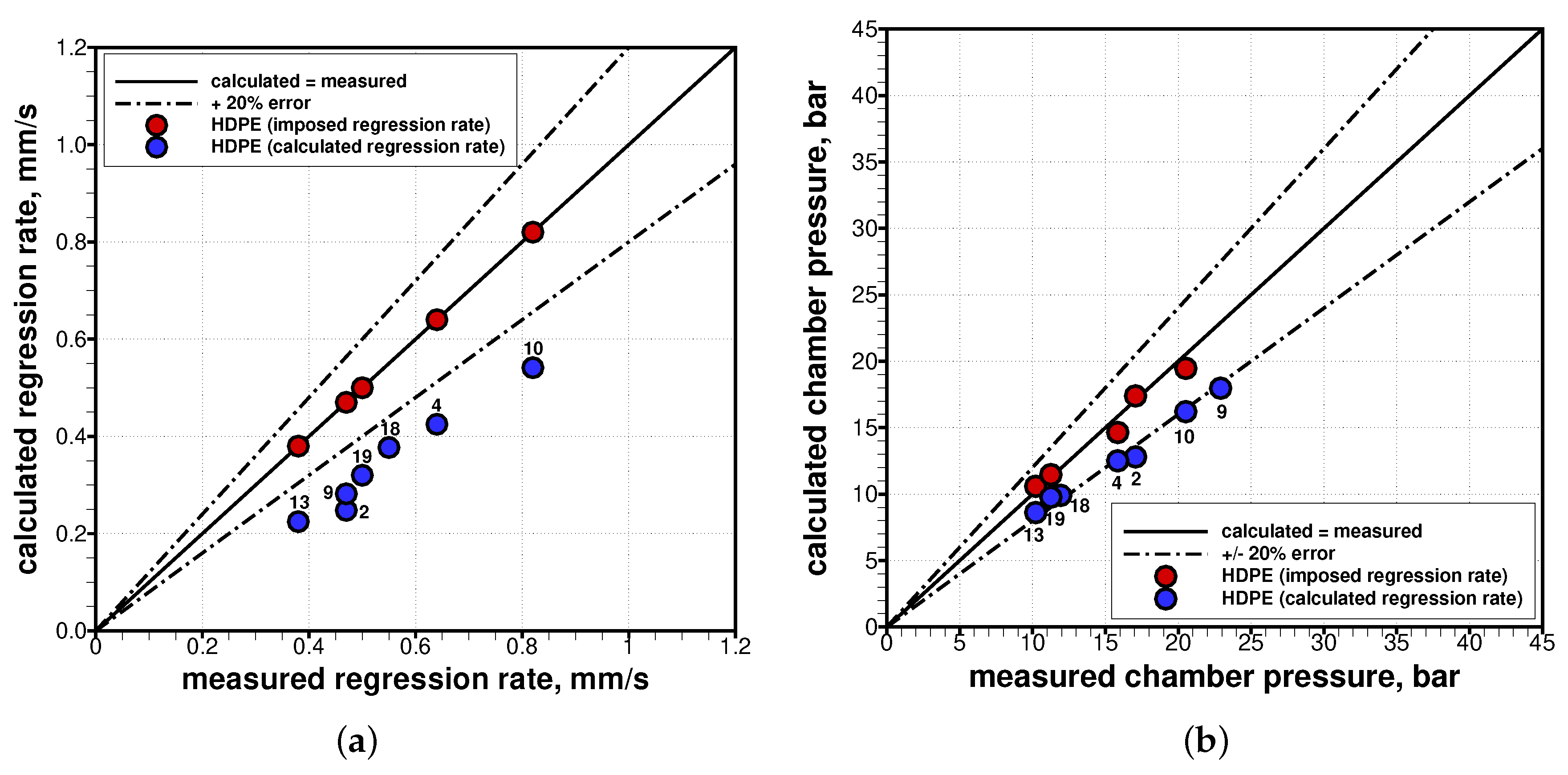
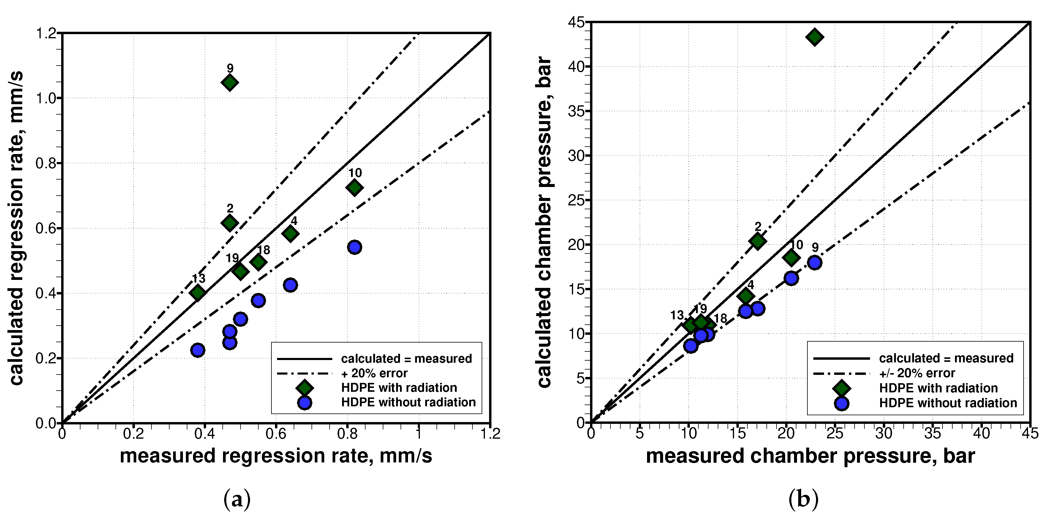
5.2. Comparison with Experimental Data

All the firing tests are considered in this section in order to understand the ability of the numerical setup to reproduce the experimental data in terms of fuel regression rate and motor chamber pressure. For such a comparison, at first, all simulations were performed neglecting radiative energy exchange and either imposing the experimental fuel regression rate or solving for the surface balances, which enabled the determination of the fuel temperature and regression rate as part of the flowfield solution. The corresponding deviation between measured and predicted data of chamber pressure and regression rate over all the firing tests are summarized in Figure 8, with both the imposed or calculated fuel regression rate. When the fuel regression rate was computed by solving the gas–surface interaction wall boundary condition (neglecting radiative energy exchange), results (see Figure 8a) indicated a quite evident underestimation of the averaged regression rate for all firing tests. This underestimation in the regression rate reflected more or less directly (depending on the average O/F ratio and on the corresponding theoretical c * of the firing test) an underestimation of the motor operating chamber pressure (see Figure 8b). In particular, the regression rate was underestimated between 31 and 47%, while the chamber pressure was underestimated between 13 and 25%. Table 11 shows the space-averaged results in terms of regression rate, chamber pressure, and convective heat flux when solving the gas–surface interaction wall boundary condition. It is important to underline here that the predicted chamber pressure was not only the result of the fuel regression rate, but also of the mixing and combustion process within the combustion chamber, which can strongly affect the characteristic exhaust velocity. Hence, a correct prediction of the fuel regression rate did not necessarily grant that the chamber pressure was correctly predicted. If the mixing and combustion processes were not correctly modeled, in fact, a mismatch between predicted and measured chamber pressure would result.
Since the previously discussed sensitivity analysis showed that the results could be affected by the law of pyrolysis adopted just for a few percentage points (less than 10% for regression rate and less than 5% for the chamber pressure), a study to evaluate the goodness of the combustion model was carried out. To check that the mixing and combustion processes were adequately modeled in the current approach, simulations for five firing tests (namely #2, #4, #10, #13, and #19) were computed by directly imposing the experimentally-measured averaged regression rate at the fuel boundary condition. Results are shown in Figure 8b in terms of motor chamber pressure and show that, once the experimentally-measured regression rate value was imposed in the simulation, a very good prediction of motor pressure (hence of the characteristic velocity) was obtained. This confirmed that mixing and combustion processes were adequately modeled in the present approach. Nevertheless, when the fuel regression rate was predicted from the gas–surface interaction wall boundary condition, the averaged regression rate values from the various experimental firing tests were always underestimated (by 31% up to 47%). Considering the analyses that were carried out so far with respect to the fuel pyrolysis model uncertainties, it is clear that such a significant underestimation must be attributed to another source of error, as the absence of the radiative contribution to the wall heating. The regression rate general trend (Figure 8a), in fact, seemed to suggest the lack of radiation modeling, whose effects are known to be more substantial at the lower oxidizer mass fluxes. Chiaverini et al. [38] showed that radiation effects are relevant for oxygen mass fluxes lower than ≈160 kg/m 2 ·s and for chamber pressures in the range 1.5 2.5 MPa or higher. The experimental conditions analyzed here were inside the indicated pressure range, and all fall well below the 160 kg/m 2 ·s for the oxygen mass flux, with three firing tests (#2, #13, and #9) reaching average values below 30 kg/m 2 ·s. Hence, the analyzed tests were expected to show significant radiation effects.

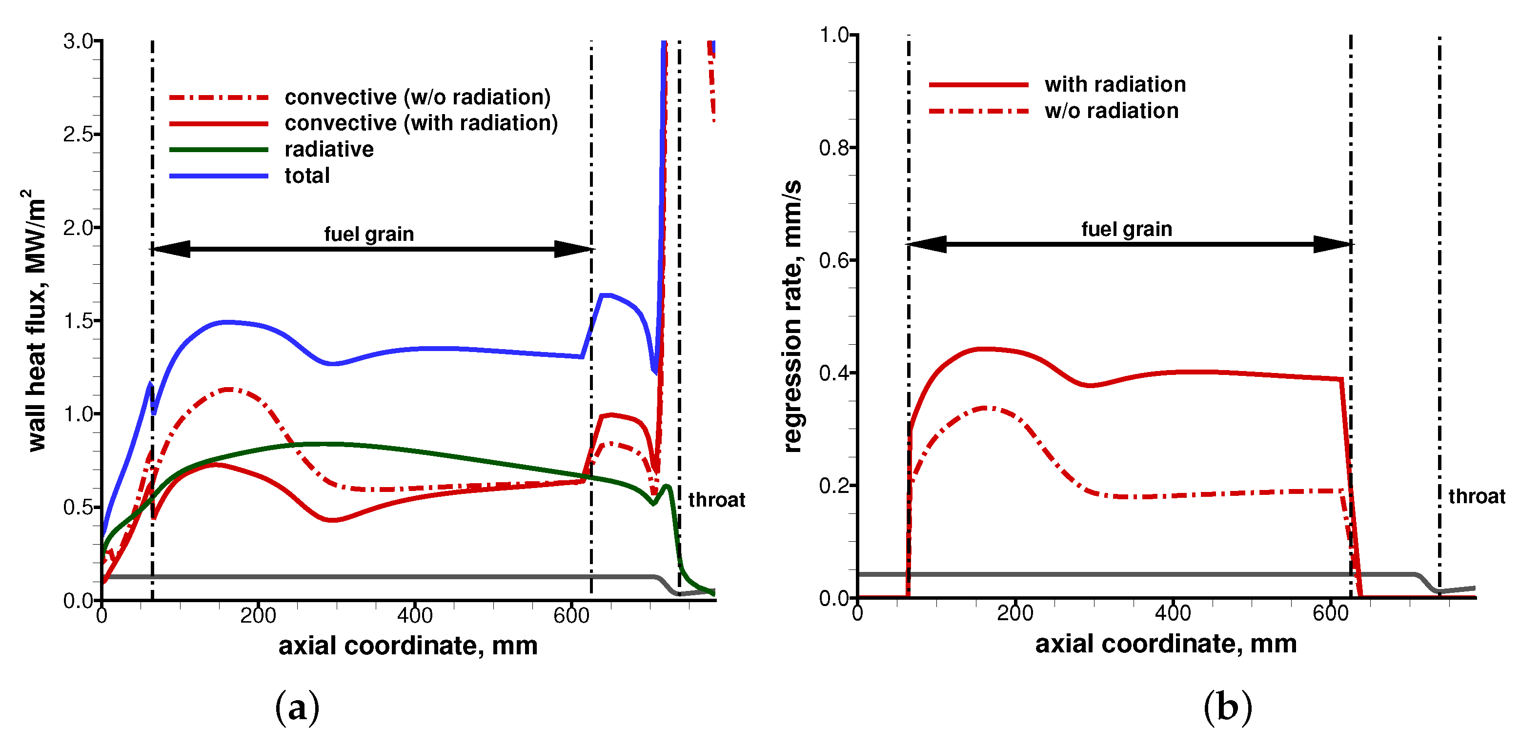
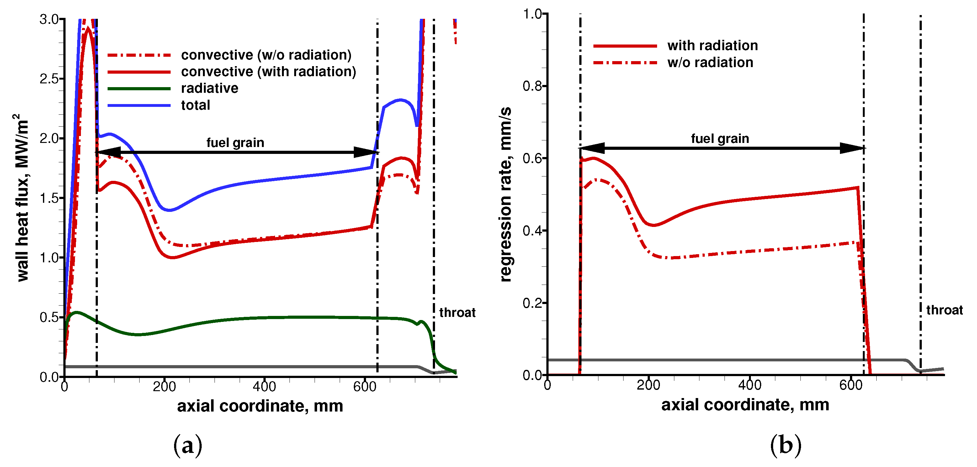
5.3. Effect of Thermal Radiation Exchange

In order to analyze the effect of radiative energy exchange, CFD simulations were coupled to radiation heat transfer calculations to take into account the net incoming radiative heat flux to the fuel grain and its effect on the fuel regression rate, through Equation (10). A wall emissivity equal to 0.85 for the HDPE grain was assumed according to typical values for polymers exposed to flames. The wall and flowfield local conditions required by the radiative simulation were taken from the CFD solution, with which the radiative solution was coupled until convergence was attained. The resulting deviation between computed (with and without radiative energy exchange) and measured data of chamber pressure and regression rate over all the firing tests is summarized in Figure 9.
Table 12 shows the space-averaged results with coupled radiative energy exchange in terms of regression rate, chamber pressure, convective heat flux, and absorbed radiative heat flux. The larger port diameter firing tests (Firing Tests #2, #9, and #13) were those for which the absorbed radiative heat flux was larger than the convective heat flux, denoting the highly non-linear contribution from thermal radiation exchange for varying operating conditions. Moreover, it is worth noting that the results obtained with coupled thermal radiation exchange (see Table 12) showed a convective heat flux that was lower than the corresponding case without radiation (see Table 11). This confirmed that, due to the well-known convective heat transfer blockage, the regression rate increase due to radiation was mitigated by a corresponding convective heat flux decrease, induced by the increased fuel blowing.
Looking at the numerical results obtained with the radiation modeling, the errors previously found without including thermal radiation were much mitigated. Despite a noticeable improvement with respect to previous solutions without radiation, the regression rate and chamber pressure for firing tests characterized by the largest port diameters (Firing Tests #2 and #9) were evidently overestimated when including thermal radiation. In particular, Firing Test #9 showed a large overestimation with respect to measured data on both the regression rate and chamber pressure data, requiring a deeper analysis of the port diameter effect on the net radiative heat flux to the grain surface. The rest of the analyzed tests, however, fell within a ±12% error on both regression rate and chamber pressure.
In particular, Figure 10 and Figure 11 show the axial distributions of convective, radiative, and total heat flux together with the fuel regression rate for Firing Test #13 (for which q ˙ ¯ rad abs was larger than q ˙ ¯ conv ) and for Firing Tests #18 (for which q ˙ ¯ rad abs was smaller than q ˙ ¯ conv ), respectively. The results highlight the coupling between radiation and the blocking effect, showing a reduction of the convective heat flux when radiation was included in the calculation. However, the effect was much stronger in the first one-third of the grain as the extra fuel injection was increasing the overall mass flux in the port, hence counteracting the blockage effect toward the aft-end of the grain. The analysis of the axial profiles also revealed that the peak of radiation heating was shifted further downstream with respect to that of convective heating, hence flattening the total incoming wall heat flux and, correspondingly, the regression rate axial distribution.
For Firing Test #9, the radiative wall heat flux was found to be much higher with respect to the other test cases as a consequence of the high value of the product between chamber pressure and port diameter. One of the causes for this significant error on the computed thermal radiation at the wall could be the simplified chemical mechanism, which lacked radicals and hence tended to overestimate both flame temperature and radiation-emitting species concentrations. Therefore, to reduce the error for the high-pressure high-diameter tests, more detailed chemical reaction mechanisms including radical species should be included to have a better prediction of the radiative heat flux. Probably, this error was also amplified in the coupling procedure between CFD and radiative simulations. In fact, as the radiation enhanced the regression rate, the mixture ratio tended to shift from an oxidizer- to a fuel-rich condition, hence increasing flame temperature and radiation-emitting species’ concentrations, which further increased the radiation contribution. Moreover, it has to be recalled that a single simulation was computed at the average port diameter, which was assumed representative of the whole firing test. This assumption might not be fully justified for firing tests characterized by a more relevant radiation exchange, which has been shown to be highly non-linear. In addition, it has been confirmed by radiative simulations [49] that the value assumed for the wall emissivity has a differential impact on the net computed radiative wall heat flux, strictly depending on the medium optical thickness, i.e., the product between chamber pressure and port diameter. In particular, for high values of the medium optical thickness, as in the case Firing Test #9, a high sensitivity to the wall emissivity was found, hence requiring more carefulness in the selection of the HDPE wall emissivity value.

6. Conclusions

A CFD approach for the internal ballistics of GOX/HDPE hybrid rocket engines integrated with gas–surface interaction modeling capabilities was presented. The fluid dynamic equations were the Reynolds-averaged Navier–Stokes equations with additional transport equations for turbulence and chemical species. Suitable sub-models were included in order to describe the homogeneous combustion in the gaseous phase, the radiative energy exchange toward the fuel surface, and the fluid–surface interaction in the fuel combustion port (fuel pyrolysis model). The gas-phase equations were solved coupled to the solid fuel-phase by using customized surface balances of energy and mass, which enabled the determination of the fuel surface temperature and regression rate as part of the flowfield solution. An experimental lab-scale test case, represented by a 1 kN-class hybrid rocket engine burning gaseous oxygen and HDPE, was simulated. A thorough sensitivity analysis was carried out on the literature pyrolysis models for HDPE. The obtained results confirmed that both the pre-exponential constant and the activation energy of the pyrolysis law had a direct effect on the grain wall temperature, while they were only mildly affecting the grain regression rate and, hence, the motor chamber pressure. This was due to the fact that the fuel temperature behaved as a compensating factor, while the regression rate was dominantly dictated by the surface energy balance. Differently, the obtained results showed a much stronger sensitivity of the fuel regression rate and chamber pressure to the value assumed for the heat of pyrolysis, which directly affected the surface energy balance. On the other hand, the effect of the heat of pyrolysis on the grain wall temperature appeared to be minimal. Thus, the pyrolysis process appeared to be definitely controlled by the energy balance at the grain surface and thus by the competition between incoming heat fluxes (convection and radiation) and outgoing heat fluxes (fuel pyrolysis and solid grain heating), with reaction kinetics only playing a minor role. The heat of pyrolysis was the parameter most affecting the fuel regression rate, followed by the activation energy with a relatively weak effect and the pre-exponential constant inducing negligibly small variations.
The numerical approach was validated by direct comparison of experimental and numerical data, in terms of time- and space-averaged measurements. The comparison revealed that, despite the adopted simplifying assumptions, the CFD approach was fairly able to capture the main features of the motor internal ballistics both in terms of regression rate and average chamber pressure trends with oxidizer mass flux and port diameter. When the experimentally-measured regression rate was imposed as a boundary condition in the simulation, the model was correctly able to predict the motor chamber pressure; hence, the mixing and combustion process were adequately modeled, with errors ranging from +4% to −8%. When the regression rate was computed from the gas–surface interaction wall boundary condition, however, the regression rate was underestimated between 31 and 47%, while the chamber pressure was underestimated between 13 and 25%. Considering the sensitivity analyses that were carried out on the fuel pyrolysis model, such a significant underestimation must be attributed to another source of error, as the absence of the radiative contribution to the wall heat flux. When a thermal radiation model was included, the errors previously found were much mitigated. Despite a noticeable improvement with respect to solutions without radiation, regression rate and chamber pressure for firing tests characterized by the larger port diameters were overestimated when including thermal radiation effects. To improve predictions, a more detailed combustion modeling including radical species was deemed necessary, as well as a deeper analysis of the port diameter and grain wall emissivity effects on the net radiative heat flux to the fuel surface. The rest of the analyzed tests, however, fell within a ±12% error on both the regression rate and chamber pressure when the radiative contribution to grain heating was included. Hence, the importance of including thermal radiation effects in the prediction of fuel regression rate and motor internal ballistics was highlighted for firing tests characterized by low oxidizer mass fluxes. Finally, the results also highlighted the coupling between radiation and the blocking effect, showing a reduction of the convective heat flux when radiation was included in the calculation, although the effect was much stronger in the first one-third of the grain and was much mitigated toward the aft-end of the grain due to the increase of the overall mass flux in the port.

Author Contributions

Conceptualization of theoretical models, D.B., G.L., F.N., M.O. and C.C.; definition of CFD models, D.B, G.L. and F.N.; implementation of CFD models, D.B. and G.L.; running of numerical simulations, D.B. and G.L.; writing–original draft preparation, D.B. and C.C.; supervision, F.N, M.O. and C.C.

Funding

This research received no external funding.

Conflicts of Interest

The authors declare no conflict of interest.

Nomenclature

athermal diffusivity, m 2 /s
cheat capacity, J/kg·K
Dport diameter, m
D i m effective diffusion coefficient, m 2 /s
Gmass flux, kg/m 2 ·s
henthalpy, J/kg
I radiative intensity, W/m 2 ·sr
kthermal conductivity, W/m·K
Lgrain length, m
m ˙ mass flow rate, kg/s
m ˙ b mass blowing rate per unit area, kg/m 2 ·s
Mmolar mass of the species, kg/kmole
Nnumber of species
O/F m ˙ o x / m ˙ f , oxidizer to fuel ratio of the motor
ppressure, N/m 2
q ˙ heat flux, W/m 2
rreflectivity
r ˙ regression rate, m/s
Runiversal gas constant, J/mol·K
sabscissa along a line-of-sight, m
Ttemperature, K
t b burning time, s
vvelocity component normal to surface, m/s
w ˙ i source term of species i in the control volume, kg/m 3 ·s
w ˙ j net reaction rate of reaction j, kmole/m 3 ·s
X i mole fraction of species i
y i mass fraction of species i
Greek
α absorptivity
ϵ emissivity
θ line-of-sight elevation angle, rad
η inward (from solid to gas) coordinate normal to the surface
κ absorption coefficient, m 1
κ p Planck-mean absorption coefficient, m 1 atm 1
ρ density, kg/m 3
σ Stefan–Boltzmann constant, W/m 2 ·K 4
ψ line-of-sight azimuth angle, rad
ω ˙ i source term of species i in the control surface, kg/m 2 ·s
Ω solid angle, sr
Subscripts
bblowing
ccombustion chamber
o x oxidizer
ffuel
ispecies
jreaction
ssolid material
wwall
Superscripts
g ¯ average in time and space
g ^ average in space

Abbreviations

The following abbreviations are used in this manuscript:
CFDComputational Fluid Dynamics
DTMDiscrete Transfer Method
GOXGaseous Oxygen
HDPEHigh-Density Polyethylene
HREHybrid Rocket Engines
HTPBHydroxyl-Terminated Polybutadiene
RTERadiative Transfer Equation

References

  1. Kuo, K.K.; Houim, R.W. Theoretical Modeling and Numerical Simulation Challenges of Combustion Processes of Hybrid Rockets. AIAA Paper 2011-5608. In Proceedings of the 47th AIAA/ASME/SAE/ASEE Joint Propulsion Conference & Exhibit, San Diego, CA, USA, 31 July–3 August 2011. [Google Scholar]
  2. Altman, D.; Holzman, A. Overview and History of Hybrid Rocket Propulsion. In Fundamentals of Hybrid Rocket Combustion and Propulsion; Kuo, K., Chiaverini, M., Eds.; Progress in Astronautics and Aeronautics; AIAA: Reston, VA, USA, 2007; Volume 218, pp. 1–36. [Google Scholar]
  3. Bianchi, D.; Urbano, A.; Betti, B.; Nasuti, F. CFD Analysis of Hybrid Rocket Flowfields Including Fuel Pyrolysis and Nozzle Erosion. AIAA Paper 2013-3637. In Proceedings of the 49th AIAA/ASME/SAE/ASEE Joint Propulsion Conference, San Jose, CA, USA, 15–17 July 2013. [Google Scholar] [CrossRef]
  4. Bianchi, D.; Betti, B.; Nasuti, F.; Carmicino, C. Simulation of Gaseous Oxygen/Hydroxyl-Terminated Polybutadiene Hybrid Rocket Flowfields and Comparison with Experiments. J. Propuls. Power 2015, 31, 919–929. [Google Scholar] [CrossRef]
  5. Cheng, G.C.; Farmer, R.C.; Jones, H.S.; McFarlane, J.S. Numerical Simulation of the Internal Ballistics of a Hybrid Rocket Motor. AIAA Paper 94-0554. In Proceedings of the 32nd Aerospace Sciences Meeting and Exhibit, Reno, NV, USA, 10–13 January 1994. [Google Scholar] [CrossRef]
  6. Sankaran, V. Computational Fluid Dynamics Modeling of Hybrid Rocket Flowfields. In Fundamentals of Hybrid Rocket Combustion and Propulsion; Kuo, K., Chiaverini, M., Eds.; Progress in Astronautics and Aeronautics; AIAA: Reston, VA, USA, 2007; Volume 218, pp. 323–349. [Google Scholar]
  7. Chen, Y.S.; Chou, T.H.; Gu, B.R.; Wu, J.S.; Wu, B.; Lian, Y.Y.; Yang, L. Multiphysics simulations of rocket engine combustion. Comput. Fluids 2011, 45, 29–36. [Google Scholar] [CrossRef]
  8. Lazzarin, M.; Barato, F.; Bettella, A.; Pavarin, D. Computational Fluid Dynamics Simulation of Regression Rate in Hybrid Rockets. J. Propuls. Power 2013, 29, 1445–1452. [Google Scholar] [CrossRef]
  9. Gariani, G.; Maggi, F.; Galfetti, L. Simulation Code for Hybrid Rocket Combustion. AIAA Paper 2010-6872. In Proceedings of the 46th AIAA/ASME/SAE/ASEE Joint Propulsion Conference, Nashville, TN, USA, 25–28 July 2010. [Google Scholar]
  10. Coronetti, A.; Sirignano, W.A. Numerical Analysis of Hybrid Rocket Combustion. J. Propuls. Power 2013, 29, 371–384. [Google Scholar] [CrossRef] [Green Version]
  11. Motoe, M.; Shimada, T. Numerical Simulations of Combustive Flows in a Swirling-Oxidizer-Flow-Type Hybrid Rocket. AIAA Paper 2014-0310. In Proceedings of the 52nd Aerospace Sciences Meeting, National Harbor, MD, USA, 13–17 January 2014. [Google Scholar] [CrossRef]
  12. Bellomo, N.; Lazzarin, M.; Barato, F.; Bettella, A.; Pavarin, D.; Grosse, M. Investigation of Effect of Diaphragms on the Efficiency of Hybrid Rockets. J. Propuls. Power 2014, 30, 175–185. [Google Scholar] [CrossRef]
  13. Kumar, C.P.; Kumar, A. Effect of Diaphragms on Regression Rate in Hybrid Rocket Motors. J. Propuls. Power 2013, 29, 559–572. [Google Scholar] [CrossRef]
  14. Di Martino, G.D.; Carmicino, C.; Savino, R. Transient Computational Thermofluid-Dynamic Simulation of Hybrid Rocket Internal Ballistics. J. Propuls. Power 2017, 33, 1395–1409. [Google Scholar] [CrossRef] [Green Version]
  15. Messineo, G.; Lestrade, J.Y.; Hijlkema, J.; Anthoine, J. Vortex Shedding Influence on Hybrid Rocket Pressure Oscillations and Combustion Efficiency. J. Propuls. Power 2016, 32, 1386–1394. [Google Scholar] [CrossRef]
  16. Arisawa, H.; Brill, T.B. Flash Pyrolysis of Hydroxyl Terminated Poly-Butadiene (HTPB) II: Implications of the Kinetics to Combustion of Organic Polymers. Combust. Flame 1996, 106, 131–143. [Google Scholar] [CrossRef]
  17. Ramohalli, K.; Yi, J. Hybrids Revisited. AIAA Paper 90-1962. In Proceedings of the AIAA/SAE/ASME/ASEE 26th Joint Propulsion Conference, Orlando, FL, USA, 16–18 July 1990. [Google Scholar] [CrossRef]
  18. Carmicino, C.; Russo Sorge, A. Influence of a Conical Axial Injector on Hybrid Rocket Performance. J. Propuls. Power 2006, 22, 984–995. [Google Scholar] [CrossRef]
  19. Bianchi, D.; Nasuti, F. Numerical Analysis of Nozzle Material Thermochemical Erosion in Hybrid Rocket Engines. J. Propuls. Power 2013, 29, 547–558. [Google Scholar] [CrossRef]
  20. Di Martino, G.D.; Mungiguerra, S.; Carmicino, C.; Savino, R. Computational Fluid-dynamic Simulations of Hybrid Rocket Internal Flow Including Discharge Nozzle. AIAA Paper 2017-5045. In Proceedings of the 53rd AIAA/SAE/ASEE Joint Propulsion Conference, Atlanta, GA, USA, 10–12 July 2017. [Google Scholar]
  21. Sutton, G.P.; Biblarz, O. Rocket Propulsion Elements; John Wiley and Sons, Inc.: New York, NY, USA, 2001. [Google Scholar]
  22. Betti, B.; Nasuti, F.; Martelli, E. Numerical Evaluation of Heat Transfer Enhancement in Rocket Thrust Chambers by Wall Ribs. Numer. Heat Transf. Part A Appl. 2014, 66, 488–508. [Google Scholar] [CrossRef]
  23. Betti, B.; Bianchi, D.; Nasuti, F.; Martelli, E. Chemical Reaction Effects on Heat Loads of CH4/O2 and H2/O2 Rockets. AIAA J. 2016, 54, 1693–1703. [Google Scholar] [CrossRef]
  24. Bianchi, D.; Nasuti, F.; Paciorri, R.; Onofri, M. Computational Analysis of Hypersonic Flows Including Finite Rate Ablation Thermochemistry. In Proceedings of the 7th European Workshop on Thermal Protection Systems and Hot Structures, ESA-ESTEC, Noordwijk, The Netherlands, 8–10 April 2013. [Google Scholar]
  25. Bianchi, D.; Nasuti, F.; Carmicino, C. Hybrid Rockets with Axial Injector: Port Diameter Effect on Fuel Regression Rate. J. Propuls. Power 2016, 32, 984–996. [Google Scholar] [CrossRef]
  26. Bianchi, D.; Kamps, L.; Nasuti, F.; Nagata, H. Numerical and Experimental Investigation of Nozzle Thermochemical Erosion in Hybrid Rockets. AIAA Paper 2017-4640. In Proceedings of the 53rd AIAA/SAE/ASEE Joint Propulsion Conference, Atlanta, GA, USA, 10–12 July 2017. [Google Scholar] [CrossRef]
  27. Gordon, S.; McBride, B.J. Computer Program for Calculation of Complex Chemical Equilibrium Compositions and Applications. NASA RP 1311; 1994. Available online: https://ntrs.nasa.gov/archive/nasa/casi.ntrs.nasa.gov/19950013764.pdf (accessed on 21 April 2019).
  28. Wilke, C.R. A Viscosity Equation for Gas Mixtures. J. Chem. Phys. 1950, 18. [Google Scholar] [CrossRef]
  29. Spalart, P.R.; Allmaras, S.R. A One–Equation Turbulence Model for Aerodynamic Flows. Rech. Aérosp. 1994, 1, 5–21. [Google Scholar]
  30. Lockwood, F.C.; Shah, N.G. A New Radiation Solution Method for Incorporation in General Combustion Prediction Procedures. Symp. Int. Combust. 1981, 18, 1405–1414. [Google Scholar] [CrossRef]
  31. Kendall, R.M.; Bartlett, E.P.; Rindal, R.A.; Moyer, C.B. An Analysis of the Chemically Reacting Boundary Layer and Charring Ablator. Part I: Summary Report; NASA CR 1060; NASA: Washington, DC, USA, 1968.
  32. Marxman, G.; Gilbert, M. Turbulent Boundary Layer Combustion in the Hybrid Rocket. Symp. Int. Combust. 1963, 9, 371–383. [Google Scholar] [CrossRef]
  33. Li, C.; Cai, G.; Tian, H. Numerical analysis of combustion characteristics of hybrid rocket motor with multi-section swirl injection. Acta Astronaut. 2016, 123, 26–36. [Google Scholar] [CrossRef]
  34. Lengelle, G.; Fourest, B.; Godon, J.; Guin, C. Condensed-phase behavior and ablation rate of fuels for hybrid propulsion. AIAA Paper 1993-2413. In Proceedings of the 29th Joint Propulsion Conference and Exhibit, Monterey, CA, USA, 28–30 June 1993. [Google Scholar]
  35. Stoiliarov, S.I.; Crowley, S.; Lyon, R.E.; Linteris, G.T. Prediction of the burning rates of non-charring polymers. Combust. Flame 2009, 156, 1068–1083. [Google Scholar] [CrossRef]
  36. Gascoin, N.; Fau, G.; Gillard, P.; Mangeot, A. Experimental flash pyrolysis of high density polyethylene under hybrid propulsion conditions. J. Anal. Appl. Pyrolysis 2013, 101, 45–52. [Google Scholar] [CrossRef] [Green Version]
  37. Lengelle, G. Solid-Fuel Pyrolysis Phenomena and Regression Rate, Part 1: Mechanisms. In Fundamentals of Hybrid Rocket Combustion and Propulsion; Kuo, K., Chiaverini, M., Eds.; Progress in Astronautics and Aeronautics; AIAA: Reston, VA, USA, 2007; Volume 218, pp. 127–165. [Google Scholar]
  38. Chiaverini, M.J.; Serin, N.; Johnson, D.K.; Lu, Y.C.; Kuo, K.K.; Risha, G.A. Regression Rate Behavior of Hybrid Rocket Solid Fuels. J. Propuls. Power 2000, 16, 125–132. [Google Scholar] [CrossRef]
  39. Chiaverini, M.J.; Kuo, K.K.; Peretz, A.; Harting, G.C. Regression-Rate and Heat-Transfer Correlations for Hybrid Rocket Combustion. J. Propuls. Power 2001, 17, 318–326. [Google Scholar] [CrossRef]
  40. Chiaverini, M. Review of Solid–Fuel Regression Rate Behavior in Classical and Nonclassical Hybrid Rocket Motors. In Fundamentals of Hybrid Rocket Combustion and Propulsion; Kuo, K., Chiaverini, M., Eds.; Progress in Astronautics and Aeronautics; AIAA: Reston, VA, USA, 2007; Volume 218, pp. 37–125. [Google Scholar]
  41. Ciottoli, P.P.; Malpica Galassi, R.; Lapenna, P.; Leccese, G.; Bianchi, D.; Nasuti, F.; Creta, F.; Valorani, M. CSP-based chemical kinetics mechanisms simplification strategy for non-premixed combustion: An application to hybrid rocket propulsion. Combust. Flame 2017, 186, 83–93. [Google Scholar] [CrossRef]
  42. Andersen, J.; Rasmussen, C.L.; Giselsson, T.; Glarborg, P. Global Combustion Mechanisms for Use in CFD Modeling under Oxy-Fuel Conditions. Energy Fuels 2009, 23, 1379–1389. [Google Scholar] [CrossRef]
  43. Muzzy, R. Applied Hybrid Combustion Theory. In Proceedings of the 8th Joint Propulsion Specialist Conference, New Orleans, LA, USA, 29 November–1 December 1972. [Google Scholar] [CrossRef]
  44. Göbel, F.; Mundt, C. Implementation of the P1 Radiation Model in the CFD Solver NSMB and Investigation of Radiative Heat Transfer in the SSME Main Combustion Chamber. AIAA Paper 2011-2257. In Proceedings of the 17th AIAA International Space Planes and Hypersonic Systems and Technologies Conference, San Francisco, CA, USA, 11–14 April 2011. [Google Scholar] [CrossRef]
  45. Jiwen, L.; Tiwari, S.N. Radiative Heat Transfer Effects in Chemically Reacting Nozzle Flows. J. Thermophys. Heat Transf. 1996, 10, 436–444. [Google Scholar] [CrossRef]
  46. Modest, M.F. Radiative Heat Transfer; Academic Press: San Diego, CA, USA, 2013; pp. 288–410. [Google Scholar]
  47. Tien, C.L. Thermal Radiation Properties of Gases. In Advances in Heat Transfer; Irvine, T.F., Hartnett, J.P., Eds.; Academic Press: New York, NY, USA, 1968; Volume 5, pp. 253–324. [Google Scholar]
  48. Rivière, P.; Soufiani, A. Updated Band Model Parameters for H2O, CO2, CH4 and CO Radiation at High Temperature. Int. J. Heat Mass Transf. 2012, 55, 3349–3358. [Google Scholar] [CrossRef]
  49. Leccese, G.; Bianchi, D.; Betti, B.; Lentini, D.; Nasuti, F. Convective and Radiative Wall Heat Transfer in Liquid Rocket Thrust Chambers. J. Propuls. Power 2018, 34, 318–326. [Google Scholar] [CrossRef]
  50. Leccese, G.; Bianchi, D.; Nasuti, F.; Stober, K.J.; Narsai, P.; Cantwell, B.J. Experimental and numerical methods for radiative wall heat flux predictions in paraffin-based hybrid rocket engines. Acta Astronaut. 2019, 158, 304–312. [Google Scholar] [CrossRef]
  51. Carmicino, C.; Russo Sorge, A. Role of Injection in Hybrid Rockets Regression Rate Behavior. J. Propuls. Power 2005, 21, 606–612. [Google Scholar] [CrossRef]
  52. Karabeyoglu, M.A.; Cantwell, B.J.; Zilliac, G. Development of Scalable Space-Time Averaged Regression Rate Expressions for Hybrid Rockets. J. Propuls. Power 2007, 23, 737–747. [Google Scholar] [CrossRef]
  53. Stoiliarov, S.I.; Walters, R.N. Determination of the heats of gasification of polymers using differential scanning calorimetry. Polym. Degrad. Stab. 2008, 93, 422–427. [Google Scholar] [CrossRef]
Figure 1. Lab-scale hybrid rocket engine schematic.
Aerospace 06 00088 g001
Figure 2. Numerical grid schematic (not to scale).
Aerospace 06 00088 g002
Figure 3. Temperature field and detail of the recirculation zone for Firing Test #19 (not to scale).
Aerospace 06 00088 g003
Figure 4. HDPE regression rate vs. temperature from various pyrolysis laws.
Aerospace 06 00088 g004
Figure 5. Effect of the pre-exponential constant on the fuel regression rate and the fuel temperature: (a) fuel regression rate; (b) fuel temperature.
Aerospace 06 00088 g005
Figure 6. Effect of the activation energy on the fuel regression rate and the fuel temperature: (a) fuel regression rate; (b) fuel temperature.
Aerospace 06 00088 g006
Figure 7. Effect of the heat of pyrolysis on the fuel regression rate and the fuel temperature: (a) fuel regression rate; (b) fuel temperature.
Aerospace 06 00088 g007
Figure 8. Comparison of computed values from simulations (with the calculated or imposed regression rate) with measured data from the experimental firings: (a) time- and space-averaged regression rates; (b) time-averaged chamber pressures.
Aerospace 06 00088 g008
Figure 9. Comparison of computed values from simulations (with and without radiative energy exchange) with measured data from the experimental firings: (a) time- and space-averaged regression rates; (b) time-averaged chamber pressures.
Aerospace 06 00088 g009
Figure 10. Axial distributions (with and without radiative energy exchange) of surface parameters for Firing Test #13: (a) convective and radiative heat flux; (b) regression rate.
Aerospace 06 00088 g010
Figure 11. Axial distributions (with and without radiative energy exchange) of surface parameters for Firing Test #18: (a) convective and radiative heat flux; (b) regression rate.
Aerospace 06 00088 g011
Table 1. Arrhenius rate constants from curve fitting for HDPE [34].
Surface Reaction A ¯ , m/s E a , kJ/mol
HDPE C 2 H 4 4.78 × 10 3 251.04
Table 2. HDPE properties [34].
Density ρ s
kg/m 3
Specific Heat c s
J/(kg·K)
Thermal Conductivity k s
W/(m·K)
Heat of Pyrolysis Δ h p
MJ/kg
960 1255.2 0.1549 2.72
Table 3. Reaction rate constants for global reactions (17) and (18).
Reaction Rate A k n k E a , k / R , K
k f 1 [5] 4.9486 × 10 9 0.015200
k f 2 [42] 2.2400 × 10 6 0.0 5032.7
k b 2 [42] 1.1000 × 10 13 −0.9739456.5
Table 4. Firing test average experimental results (HDPE) [51].
Test No. t b , s G ¯ ox , kg/m 2 · s D ¯ , mm r ˙ ¯ , mm/s p ¯ c , bar O / F ¯
2 54.9 27.68 75.84 0.47 17.07 2.05
4 43.0 87.14 43.48 0.64 15.84 2.70
9 31.5 28.41 89.84 0.47 22.91 2.50
10 21.2 126.00 42.33 0.82 20.52 3.02
13 26.2 28.19 60.04 0.38 10.22 2.05
18 44.1 78.07 40.32 0.55 11.94 2.64
19 44.3 54.03 47.19 0.50 11.26 2.37
Table 5. Activation energies and pre-exponential constants for different HDPE pyrolysis laws (Equation (16)).
Pyrolysis LawSource A ¯ , m/s E a , kJ/mol
r1 (reference)[34,51] 4.78 × 10 3 251.04
r2[33] 2.68 × 10 3 251.20
Table 6. Activation energies and pre-exponential factors for different HDPE pyrolysis laws (Equation (14)).
Pyrolysis LawSourceA, 1/s E a , kJ/mol
r3[34] 2.00 × 10 16 251.04
r4[35] 4.80 × 10 22 349.00
r5[36] 7.57 × 10 6 130.00
Table 7. Computed average results for Firing Test #19 with the effect of a change in the pre-exponential constant, Case #19a.
Firing Test p c ¯ , Bar r ˙ ¯ , mm/s
#199.780.320
#19a9.69 (−0.9%)0.316 (−1.3%)
Table 8. Computed average results for Firing Test #19 with the effect of a change in the activation energy, Case #19b.
Firing Test p c ¯ , Bar r ˙ ¯ , mm/s
#199.780.320
#19b9.25 (−5.4%)0.283 (−11.6%)
Table 9. Computed average results for Firing Test #19 with the effect of a change in the heat of pyrolysis, Case #19c.
Firing Test p c ¯ , Bar r ˙ ¯ , mm/s
#199.780.320
#19c10.37 (+6.0%)0.387 (+20.9%)
Table 10. Computed average results for Firing Tests #2 and #10 with the effect of a change in the pyrolysis law data (r1 vs. r4), Cases #2d and #10d.
Firing Test p c ¯ , Bar r ˙ ¯ , mm/s
#2 (r1)12.780.248
#2d (r4)13.23 (+3.5%)0.265 (+6.9%)
#10 (r1)16.260.541
#10d (r4)17.01 (+4.6%)0.589 (+8.9%)
Table 11. Computed average results (gas–surface interaction w/o radiation).
Test No. r ˙ ¯ , mm/s p ¯ c , Bar q ˙ ¯ conv , MW/m 2
2 0.25 12.80 0.83
4 0.42 12.51 1.43
9 0.28 17.97 0.94
10 0.54 16.21 1.86
13 0.22 8.61 0.75
18 0.38 9.91 1.28
19 0.32 9.77 1.07
Table 12. Computed average results (gas–surface interaction with radiation).
Test No. r ˙ ¯ , mm/s p ¯ c , Bar q ˙ ¯ conv , MW/m 2 q ˙ ¯ rad abs , MW/m 2
2 0.62 20.38 0.50 1.59
4 0.58 14.20 1.34 0.64
9 1.05 43.31 0.38 3.22
10 0.72 18.52 1.74 0.73
13 0.40 10.92 0.59 0.76
18 0.50 10.96 1.22 0.46
19 0.47 11.22 0.96 0.61

