Preliminary Design and System Considerations for an Active Hybrid Laminar Flow Control System

Abstract

Hybrid laminar flow control or HLFC design is a complex and multi-disciplinary process, which demands a thorough understanding of all aspects from a global systems viewpoint. The objective of the paper is to present a preliminary design of important components of an HLFC system that helps in quick assessment of conceptual system architectures. This is important to evaluate feasibility, system performance, and overall aircraft benefits at early stages of system development. This paper also discusses the various important system requirements and issues concerning the design of active HLFC systems, and the interfaces between various disciplines are presented. It can be emphasized from the study that the future compressor design for the HLFC system should consider the thermal management aspects and additional mass flow requirements from the aerodynamics-structure design optimization and also from water drain system solutions. A method to calculate the accumulated water content inside the plenum chambers is presented, and the effect of a drain hole on the power consumption is studied. A low order thermal management study of the HLFC compressor motor shows a high temperature rise in the windings for very high speed motors for long duration operation and calls for effective cooling solutions.

1. Introduction

The aviation industry contributes a lot to carbon dioxide (CO₂) emissions and the research trend in the 21st century is towards environmentally sustainable aviation. Reducing the drag, and hence fuel burn, is one of the main objectives to reach the CO₂ reduction targets of ACARE’s Horizon 2020 and Flightpath 2050. Besides the environmental benefits, the forecast of increasing fuel prices leads to the demand for more fuel efficient aircraft to reduce the direct operating costs. Drag reduction can be achieved by keeping the flow in the boundary layer over the aircraft surfaces (wing, horizontal tail plane (HTP), vertical tail plane (VTP), engine nacelles, and fuselage) laminar, rather than the usual turbulent boundary layer flow [1]. A laminar boundary layer flow has approximately ten times lower friction drag than a turbulent boundary layer flow, and approximately 50% of the total aircraft drag during cruise comes from friction drag [2]. The techniques to delay the transition from a laminar to a turbulent boundary layer flow can be separated into natural laminar flow (NLF), laminar flow control (LFC), and hybrid laminar flow control (HLFC), as shown in Figure 1. An NLF airfoil possesses a favorable pressure gradient in order to delay the transition. The limiting factor is the sweep angle of the wing, which is usually increased for higher cruise Mach numbers. A higher swept wing is vulnerable to crossflow instabilities, which cannot be countered by merely influencing the pressure distribution [1,3]. For conventionally swept wings of high-speed aircraft, the transition point can be delayed by removing air through boundary layer suction to damp aerodynamic instability mechanisms such as Tollmien–Schlichting instability and crossflow instability [1]. The LFC technique, in which the air is sucked over the entire wing, has the disadvantages of causing structural issues when interfering with the wing box and the available space for fuel is reduced due to the complex and heavy suction system [2].

HLFC combines NLF and LFC, by which instability mechanisms can be damped and the transition can be shifted beyond 50% chord [4]. Furthermore, the suction system complexity and power consumption are decreased. The HLFC system can either be passive (requiring no continuous energy input) or active (requiring energy input). It reduces aircraft skin friction drag by boundary layer suction along the leading edge, and has been investigated in research institutions and industry since the 1970s [1,5]. The first commercial aircraft, modified with an HLFC system for flight test purposes, was equipped with a heavy suction system to be as flexible as possible [6]. Recent research papers investigate system benefits for novel HLFC concepts [7,8] for the VTP.

In the context of the European Union (EU) Clean Sky 2 (grant number: 807097–LPA GAM 2018) project named ECHO (Evaluation of Certified HLFC Elevator in Operation), suction system concepts for the horizontal tail plane (HTP) of Airbus A350 aircraft have been evaluated. An approach was developed to evaluate active type suction systems and, also, the various issues associated with it were discovered.

Though sizing methodologies for the preliminary design of the active suction system were developed by Pe [9], the focus of optimization lies on single aspects rather than considering a holistic approach, and also there is a gap in estimating the size and mass of the compressor(s), particularly for the HLFC system operating conditions. The knowledge about the approximate size of the compressor helps in evaluating the feasibility of a concept at an early stage of system development. So far, no specific challenges related to active HLFC system design is reported in literature. This paper addresses the gap and presents a way to quickly assess HLFC system concepts and discusses the important aspects of active HLFC system design.

Section 2 explains the suction system requirements and interfaces between the various disciplines. Section 3 presents the generalized description of the HLFC suction systems design approach. Section 4 explains the special challenges related to active-type suction systems with a specific case study. Section 5 presents the discussion and conclusion part.

2. Requirements, Interfaces, and Assessment Method for Active HLFC Suction System

The suction system is the central part of the HLFC system architecture. To achieve suction, a pressure difference needs to be created between the airfoil surface and the plenum beneath it. The pressure difference can be established by an active system, e.g., compressors, or by a passive system which utilizes the natural pressure differences occurring between the airfoil surface and the outlet position. The surface of the suction areas must be slotted or perforated to remove air from the boundary layer (Figure 2). Advanced manufacturing techniques are necessary to create perforations in a titanium (Ti) sheet and to bond it with the CFRP (carbon fiber reinforced plastic) leading edge structure.

Some of the important suction system requirements and the interfaces associated with the system design are described below.

2.1. Suction System Requirements

The compressor is an important component of the active-type HLFC system and a proper configuration that satisfies all the specification requirements needs to be selected. From a systems point of view, the suction system should satisfy the following basic requirements:

• Installation:

  ○

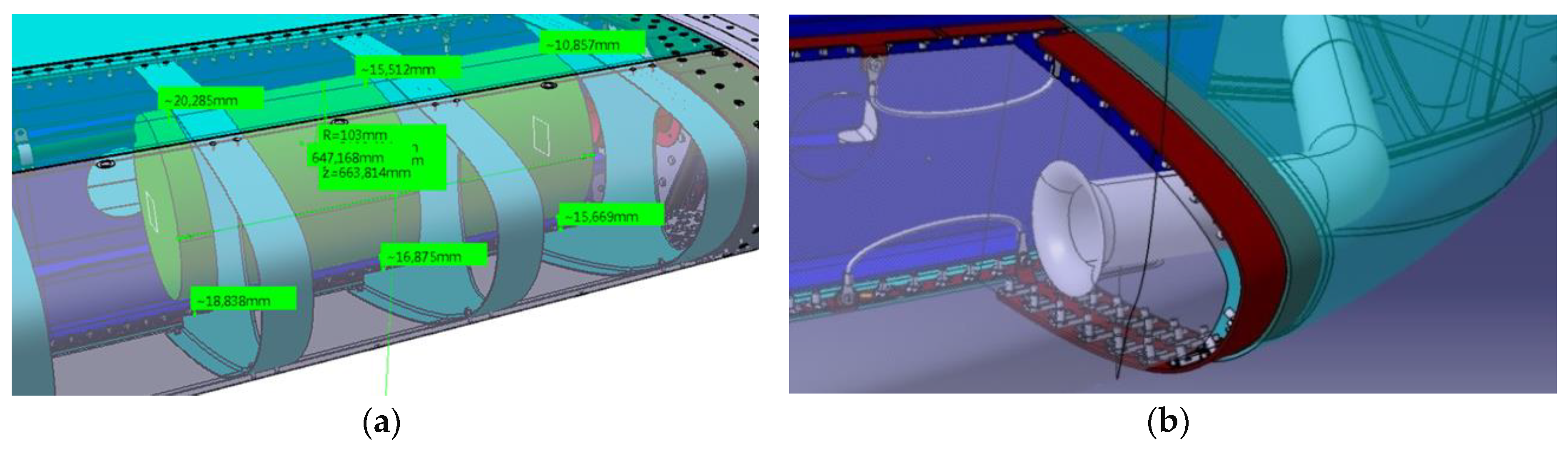
  The size of the compressor + motor arrangement should satisfy system spatial requirements. Space allocation for all suction system equipment needs to be provided.

  ○

  Routing of electrical cables should be foreseen.

  ○

  External aircraft structural movement shall NOT be affected by installed parts.

  ○

  The suction system should comply with RTCA/DO 160 [11].

  ○

  The suction system shall cope with hail impact.

  ○

  Drainage of fluids shall be ensured.

• Performance:

  ○

  The selected compressor + motor arrangement should satisfy the mass flow and pressure ratio requirements.

  ○

  The compressor + motor arrangement should possess high efficiency, so as to keep power off-takes at a minimum.

  ○

  Large rotor length-to-diameter ratio is desirable for the electric motor, as it minimizes the rotor inertia, thus maximizing the motor acceleration.

• Operational:

  ○

  Abnormal system activities should be detected and indicated.

  ○

  Status monitoring information for pre-flight, in-flight Go/No-Go, and diversion decisions.

  ○

  The suction system should operate within the aircraft operating envelope.

• Safety:

  ○

  Dispatchability with a single failure should be possible.

  ○

  No single failure shall lead to catastrophic conditions (necessary redundancies shall be considered).

  ○

  The HLFC system shall be protected against lightning effects, electro-magnetic interference (EMI), high intensity radiated field (HIRF), and electro-static discharge (ESD).

  ○

  The compressor must have cooling, so that the electric and electronic components do not overheat.

  ○

  Compliance with requirements imposed with Particular Risk Analysis (PRA) needs to be considered.

  ○

  Equipment should have good durability.

• Thermal Requirements for HLFC System Components

In addition to the above basic requirements, an important factor to be considered in the active HLFC system design is the thermal management of the components. The HLFC system operates in cruise conditions continuously for a time range of 6–10 h. The suction system components, namely the electric compressor and the power electronic components, may experience heating problems. Such increase in temperatures has the potential to damage the components or could cause a fire scenario. One of the main components that could get overheated is the motor running the compressor. The smaller size of high rotations per minute (RPM) machines (which is also a necessity for HLFC system with regard to space allocation) makes it challenging to make a cooling arrangement. Since the HLFC system operates at high altitudes, it is expected that the outside temperature helps in cooling of the components. However, it is important to know that the air density is lower at high altitudes, which makes it very thin and hence convection type cooling may not be very effective. Similar cooling arrangements should also be considered for the associated power electronic components.

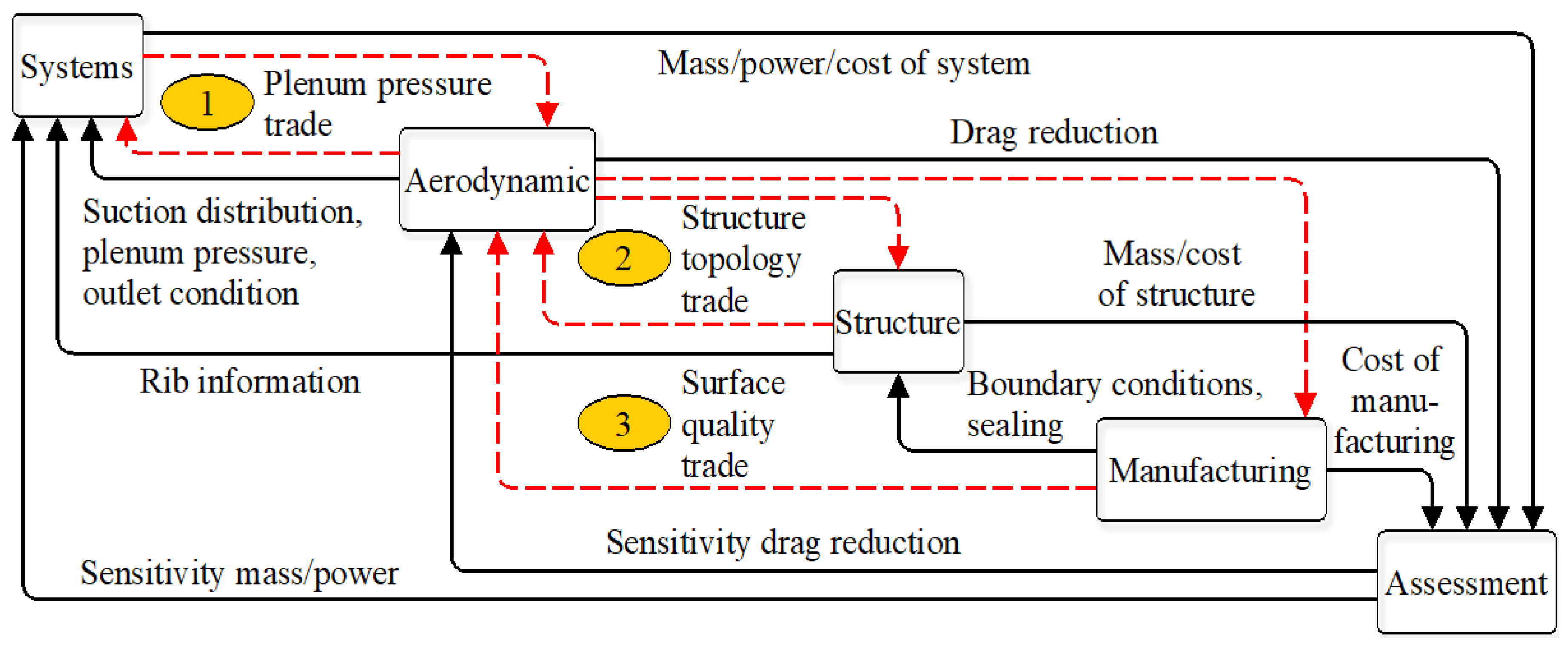
2.2. Interfaces in the HLFC System Design and Assessment Method

In the design of an HLFC system, multiple disciplines are involved, which increases the challenge to develop a completely optimized system [12]. In the following, the main disciplines and tasks are presented and their interfaces are outlined. The ALTTA concept (Figure 3) is taken as a reference HLFC concept, which is also considered for the ECHO project. In this concept, the leading edge structure has a dual layer, the outer sheet is the micro-perforated porous surface, and the inner sheet consists of orifices for the air to enter the plenum chamber, which is connected to the compressor leading to the exhaust. The leading edge surface is separated into many chambers chordwise with width W and height H.

Aerodynamics: The aerodynamics discipline performs laminar/turbulent transition calculations to obtain the spanwise and chordwise boundary layer suction speed. Furthermore, this discipline details a chambering concept (Figure 3). The spanwise and chordwise position of a suction area is also defined through transition calculations. The main aerodynamic inputs are the optimized parameters such as plenum pressure necessary to maintain suction during the system operation, the required mass flow, and the relevant operating condition parameters such as design point altitude, temperature, pressure, etc.

Structure: The structure discipline defines a suitable structural concept in the leading edge. The wing or tail plane structure has to withstand gust loads, as well as a bird strike impact and hail strike. Additional laminar requirements have to be accounted for, like aerodynamic constraints regarding surface waviness. A bonding concept for the different components is defined, e.g., stringers to the perforated skin. Furthermore, structural concepts for joining the leading edge to the wing box (chordwise direction), as well as between the leading edge panels (spanwise direction), have to be designed. It is tried to minimize the weight of the new structural concept in order to maximize HLFC benefits compared to a turbulent design. The structure’s group provides various inputs regarding the geometry of the suction system, bonding strategies, and space constraints for placing the compressor and the peripherals such as electric harness, converters, etc.

Manufacturing: The manufacturing discipline chooses the material and drilling process for the micro-perforated surface—the material has to be robust to withstand severe flight conditions (such as bird/hail strike, icing, impact with foreign objects, etc.) while keeping laminar constraints (hole geometry and surface quality). It details the laminar joint based on trade studies with the aerodynamics discipline regarding step, gap, and overlap. Additionally, sealing concepts between the leading edge and the wing box, as well as between individual chambers, are detailed.

Systems: The systems discipline designs and assesses system concepts based on aerodynamic, structural, and operational constraints. This includes the design and integration of the suction system and other subsystems, like draining system, anti-contamination system, or control and monitoring system. Integration studies need to be performed, keeping the safety and reliability of the various subsystems in the constrained space of the leading edge in mind to comply with relevant regulatory requirements.

At the conceptual stage, several system concepts need to be assessed for performance and feasibility, as shown in Figure 4. With the relevant inputs from other disciplines, the HLFC system concepts can be generated and evaluated. The main calculated parameters are the system power consumption, system mass, compressor and motor size and mass, as well as the technical feasibility of the architectures. The technically feasible concepts can then be selected by doing a trade-off between all the evaluated system concepts, and the overall aircraft benefit assessment can then be performed to estimate the drag reduction, fuel estimation, and cost assessment for the overall system.

Figure 5 graphically presents the disciplines and the exchanged information. Black arrows are one-way information, like the mass, power, or cost of the system to the overall assessment discipline. Red arrows show main interdisciplinary iterative processes. Only if all iterative loops are considered can an overall optimized HLFC system be realized.

(1)

Plenum pressure trade—between the systems and the aerodynamics disciplines, the effect of the plenum pressure tolerance has to be evaluated. The effect of a narrower plenum pressure tolerance has to be compared to the additional system cost.

(2)

Structure topology trade—between the structure and the aerodynamics disciplines, the structural concepts have to be evaluated. The thickness of the stringers is an important factor for the structural stiffness, as well as for the suction distribution (at structural elements suction is not possible).

i

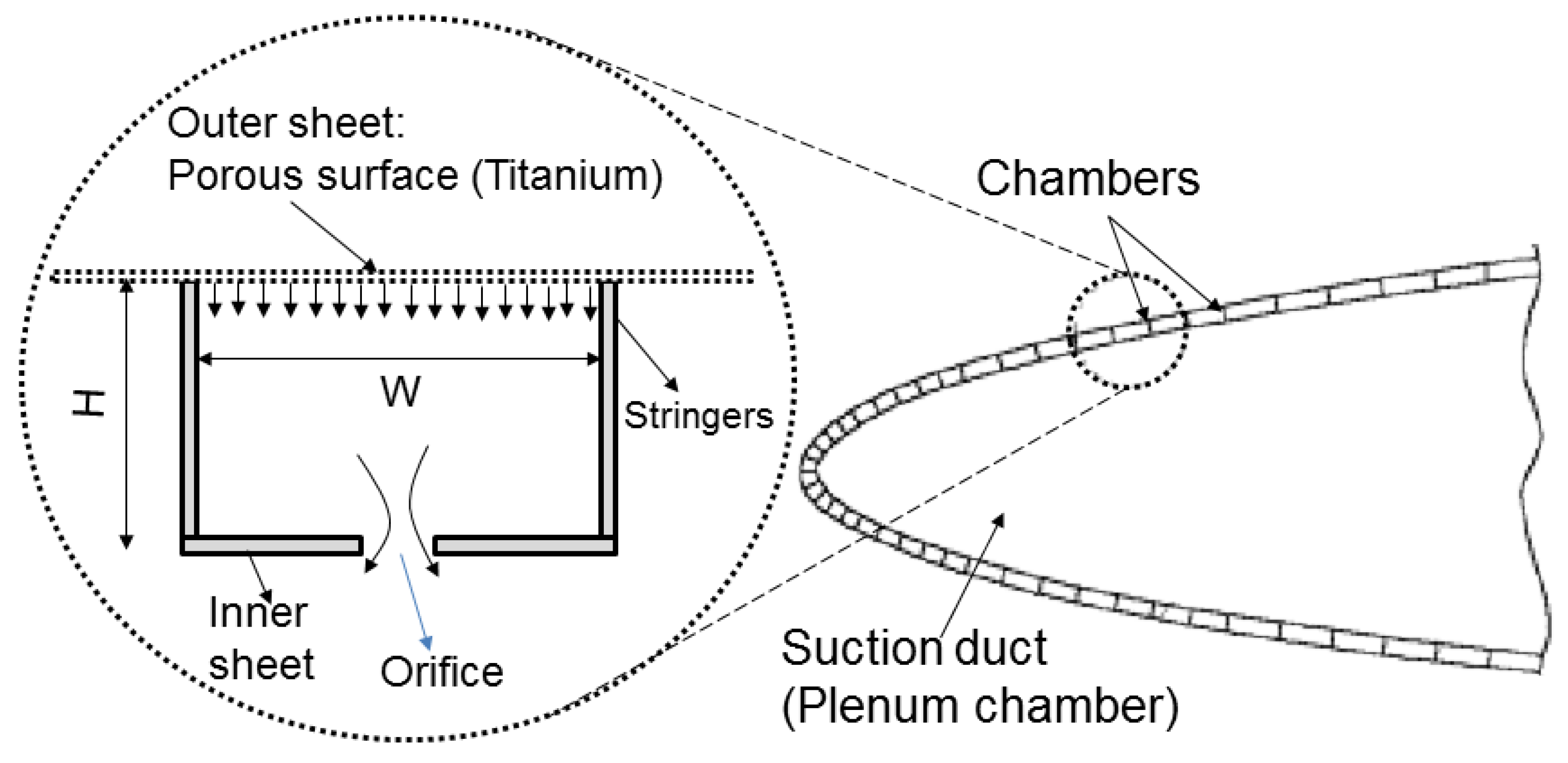
Chamber layout trade: A trade-off should be made between the aerodynamics, structures, and manufacturing disciplines on the chamber layout (number of chambers, chamber width W, chamber height H). The number of chambers should be optimized, both aerodynamically and structurally. The parameter chamber height H affects the flow velocity $v_0$ through the chambers and stress on the leading edge structure. It also has to be validated for manufacturing feasibility. Finally, a trade-off is required between the throttle orifice diameter $d_{orifice}$ and the number of throttle orifices $n_{orifice}$. A change in the chamber layout affects the mass flow rate, and hence the system suction power. The change in mass flow rate after the chamber optimization is given by $\Delta {\dot{m}}_{chamber\_opt}$.

ii

Rib structure trade: The ribs are necessary to provide strength and support to the leading edge structure. The choice of the rib structure is a trade between structure, manufacturing, and systems aspects. Most importantly, the bird strike/foreign object impact is the main criterion for the rib structure selection. From experiences gained in the Clean Sky 2 ECHO project, it is seen that the pressure loss due to ribs ($\Delta p_{ribs}$ is often negligible. Other than the rib strength, system installation such as routing of electrical harness can be considered as secondary criteria in rib structure selection. Stress effects of ribs on the perforated surface need to be assessed from a manufacturing view-point.

(3)

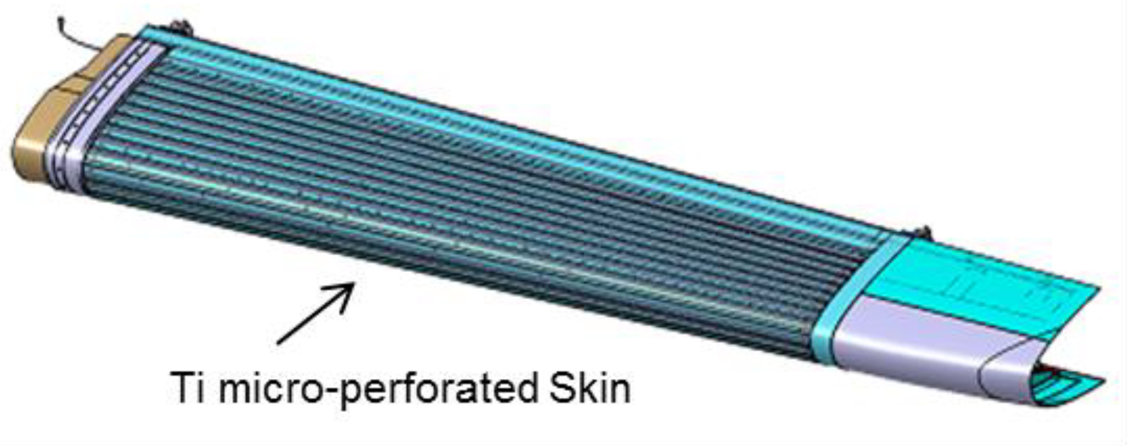
Surface quality trade—trade studies between the manufacturing of the micro-perforated outer skin and aerodynamic requirements need to be performed. The hole quality, conicity based on the discharge coefficient ($C_d$), which is the ratio of the actual discharge to the theoretical discharge, and symmetry play an important role in the aerodynamic qualification of the perforated surfaces. Furthermore, requirements for gaps, steps, and overlap need to be traded between economically viable manufacturing methods and aerodynamic constraints.

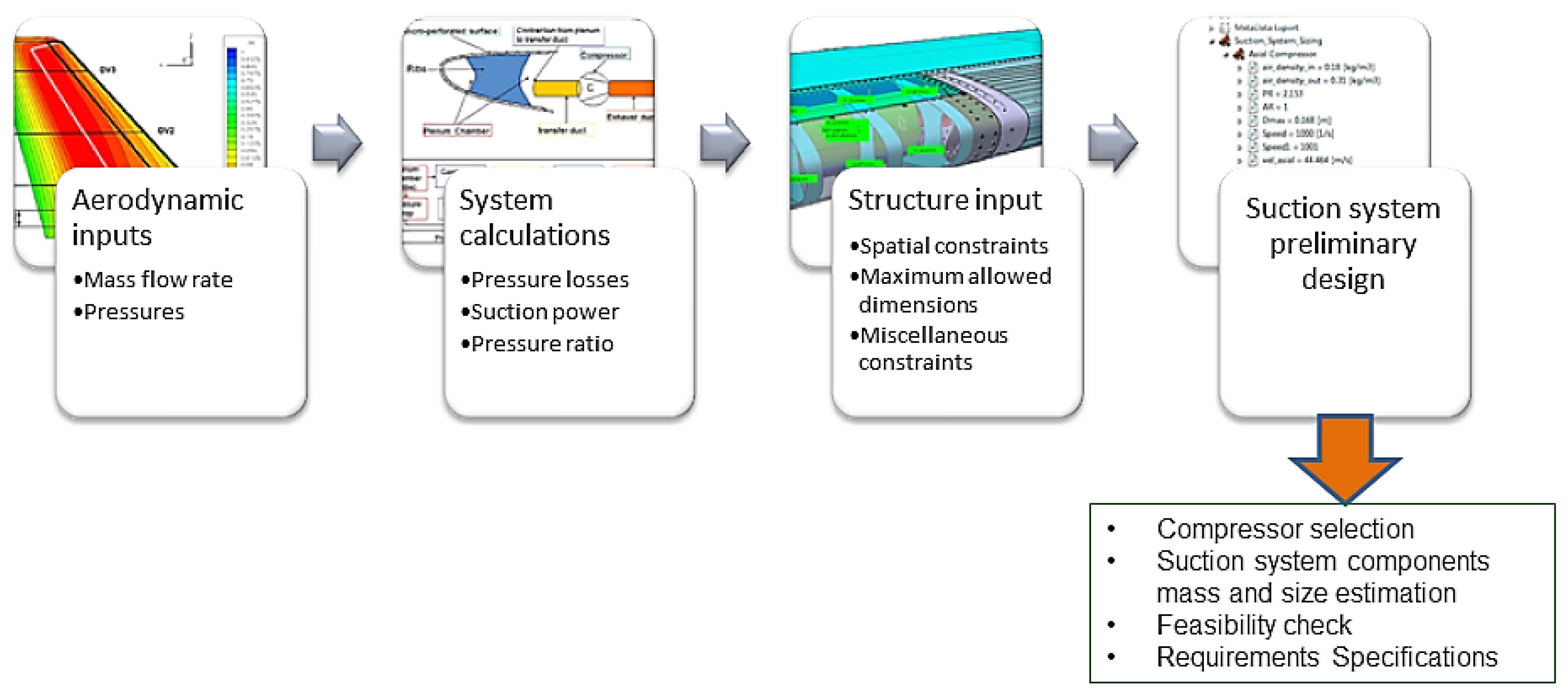
3. Active Suction System Preliminary Design Approach

The suction system design approach for an active HLFC system is shown in Figure 6. The starting point is the set of optimized aerodynamic parameters for the suction system, namely the mass flow requirements, the pressure distribution over the wing, HTP, or VTP, and the plenum chamber pressures, along with the input from the structural discipline regarding the space constraints.

The pressure losses in the ducts, duct design, suction power and power off-takes, compressor design, and suction system total mass are then calculated in the system concept evaluation calculations. With the calculated suction power and power ratio, and for a given mass flow requirement (from aerodynamic calculations), a compressor is selected and the mass and size are estimated. Finally, the design is checked in the digital mock-up to see if the spatial constraints are satisfied. Once all of the possible system concepts are evaluated, the compressor specification document for the most feasible concept is made. For the preliminary design of the compressors, the outflow/exhaust position is important, as it influences the length, complexity, and mass of the ducting and power consumption. Some of the possibilities for compressor outflow are discussed below:

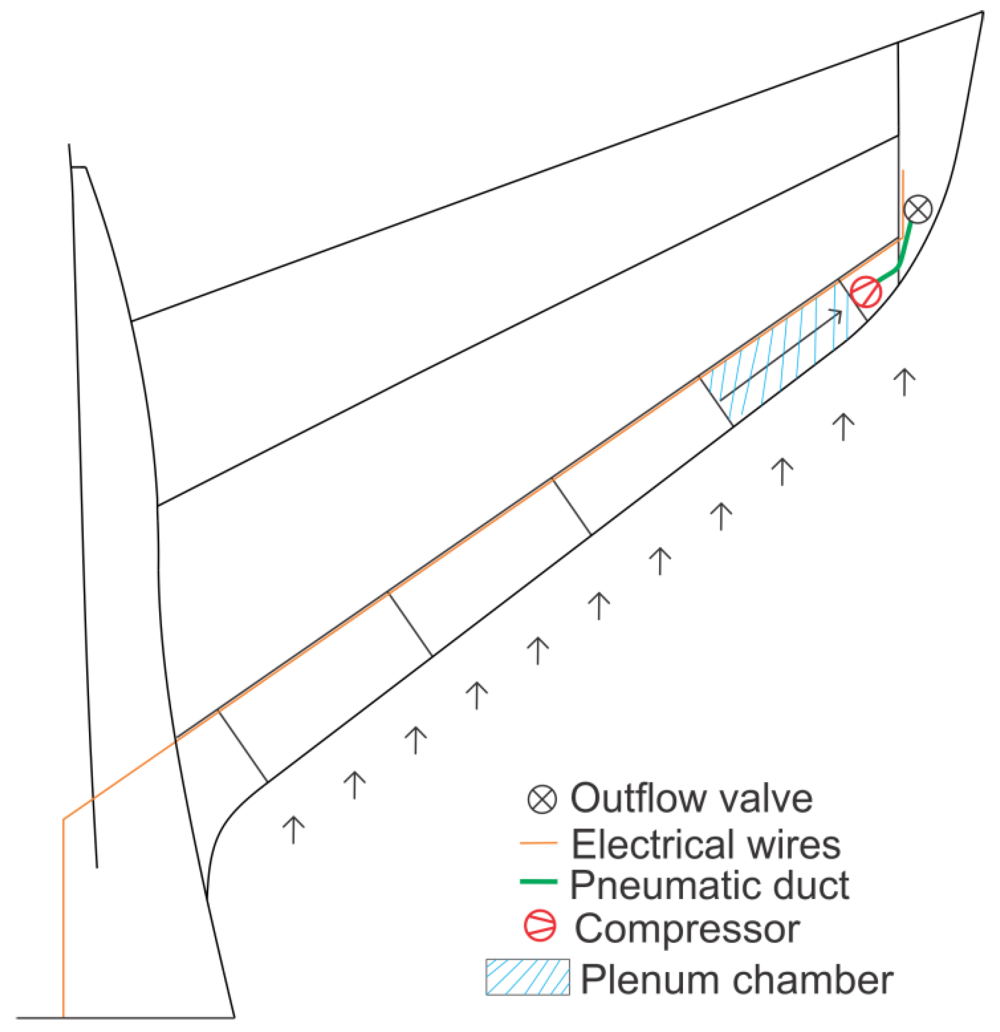
• The first possibility for the compressor outflow is letting the exhaust gas escape to the outside environment. At this outflow position, the static pressure in the duct must be equal to or greater than the static pressure at the surface to allow the air to flow out of the system.
• The second possibility is connecting the compressor outflow to the engine, adding a bit more thrust to the engines, though this thrust value is very small compared to the jet engines.
• The third possibility for using the compressor outflow is to connect the compressor exhaust gas to the bleed air ducts, which can either be used for environmental control systems or for wing ice protection systems (WIPS). This possibility of connecting the compressor outflow for usage in WIPS could be considered for HLFC applications especially in the wing area, as there is a strong need for icing solutions.

The calculations performed in this paper consider the compressor exhaust gases escape to the outside environment. Hence, the static pressure $P_{static}$ near the exhaust port needs to be considered for the compressor design calculations.

The total system mass of the HLFC system can be estimated as follows:

$$m_{HLFC\_system}=m_{compressor}+m_{motor}+m_{VFD}+m_{electric\_harness}+m_{transfer\_duct}+m_{exhaust\_duct}$$

(1)

where $m_{compressor}$, $m_{motor}$, $m_{VFD}$, $m_{electric\_harness}$, $m_{transfer\_duct}$, $m_{exhaust\_duct}$ are the mass of HLFC compressor, mass of motor, mass of power supply unit/variable frequency drive (VFD)/inverter, mass of electric harness, mass of transfer duct, and mass of exhaust duct, respectively. To solve Equation (1), it is necessary to estimate the masses of HLFC system components such as the compressor, motor, electrical harness, power electronics, and the pneumatic ducts. For mass estimation, it is necessary to evaluate the power consumption of the suction system. The Nomenclature section explains all the used parameters in the calculations.

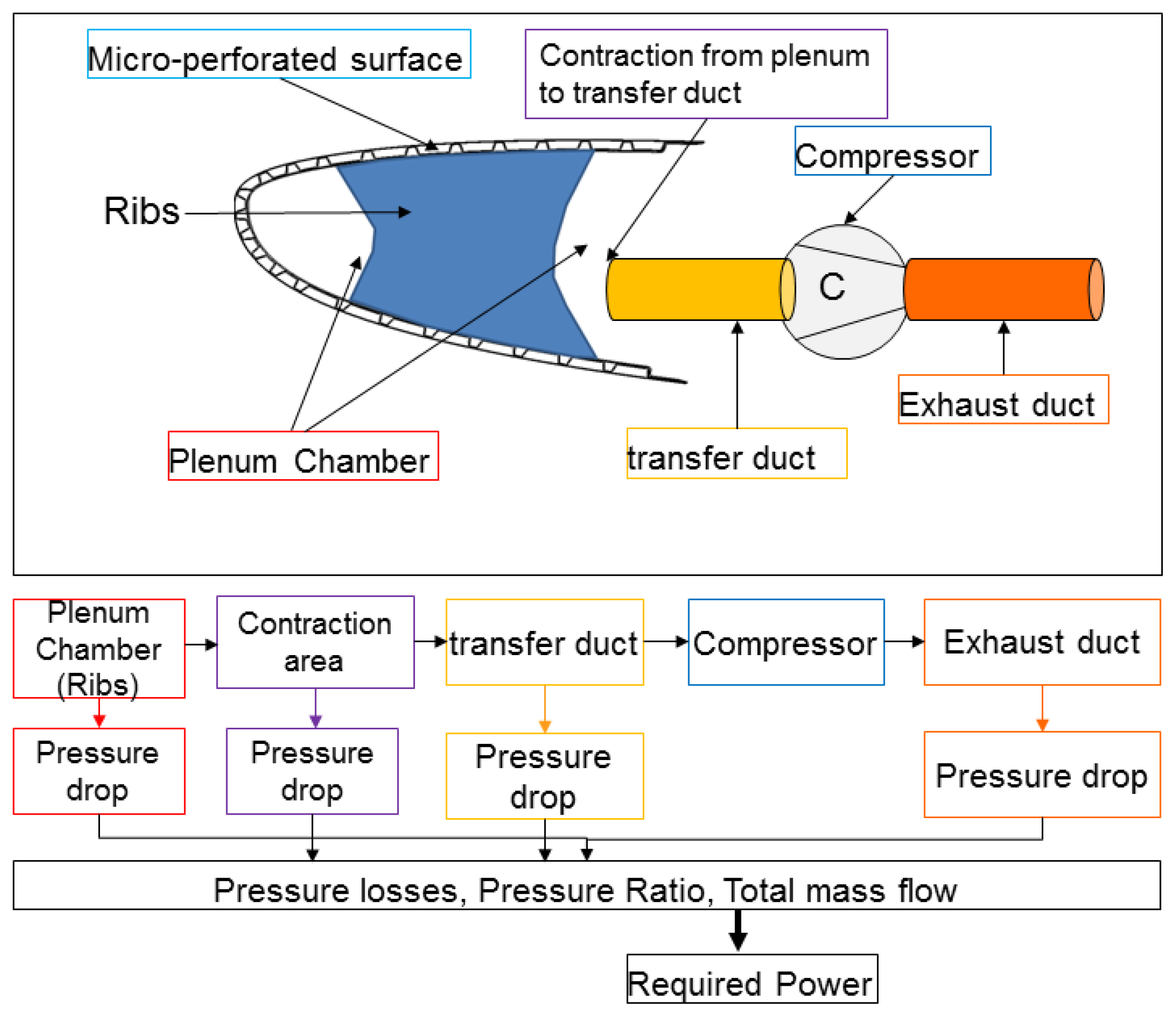
3.1. Suction System Power Consumption Estimation

The schematic in Figure 7 explains the various pressure losses occurring in the suction system and the subsequent calculation of suction power requirements (idealized isentropic flow is assumed for calculation purpose).

The pressure drop for an active HLFC system concept mainly occurs in the transfer duct and in the exhaust duct. The pressure in the plenum stays almost constant, while having a negligible pressure drop due to the presence of ribs. The flow through the ribs can be treated as a flow through a uniformly distributed barrier [13] and the pressure loss is given by Equation (2).

$$\Delta p_{ribs}={\zeta }_{rib}{\rho }_{inlet}\frac{v_0{}^2}{2}$$

(2)

where $v_0$ is the flow velocity, ${\rho }_{inlet}$ is the inlet air density, and the resistance coefficient (${\zeta }_{rib}$) is given by

$${\zeta }_{rib}=\frac{1-\overline{f}}{\overline{f}}$$

(3)

where $\overline{f}$ is the ratio of the free rib area ($F_{ribs\_free}$—where flow can pass through) to the total area at the rib ($F_{ribs\_total}$).

The air transport from the plenum chamber to the compressor via the transfer duct is associated with contraction, and hence, contraction pressure loss [13] is given by Equation (4).

$$\Delta p_{contra}=\frac{{\rho }_{in}}{2}{v}_1{}^2·0.5·{\left(1-\frac{F_1}{F_0}\right)}^{\raisebox{1ex}{$3$}\!\left/ \!\raisebox{-1ex}{$4$}\right.}$$

(4)

where $v_1$ is the flow velocity downstream of the contraction, and $F_0$ and $F_1$ are the cross-sectional areas upstream and downstream of the contraction, respectively. Another kind of pressure loss happens in the transfer and exhaust ducts. In order to determine the pressure ratio for the compressor, it is important to determine the pressure at the inlet and outlet of the compressor. This can be calculated only if the pressure losses in both upstream and downstream conditions are known. The losses in the transfer duct can be estimated using Equation (5).

$$\Delta p_{transfer\_duct}={\zeta }_{transfer\_duct}·{\rho }_{in}·\frac{v^2}{2}={\lambda }_{transfer\_duct}·\frac{L}{D_h}·{\rho }_{in}·\frac{v^2}{2}$$

(5)

where L is the length of the pipe, the pipe friction coefficient ${\lambda }_{transfer\_duct}$ depends on the ratio between the wall roughness k and the product of the diameter and the Reynolds number. For non-circular components, the hydraulic diameter $D_h$ is $D_h=\frac{4·A}{U}$, where A is the surface area and U the wetted perimeter [13].

The compressor inlet pressure can now be computed by subtracting all the pressure losses from the plenum pressure.

$$P_{in}=P_{plenum}-\Delta p_{ribs}-\Delta p_{contra}-\Delta p_{transfer\_duct}$$

(6)

Once the pressure losses are estimated, the pressure ratio for the compressor can be determined as the ratio between pressure at the compressor inlet $P_{in}$ and the pressure at the compressor outlet $P_{out}$.

$$PR=\frac{P_{out}}{P_{in}}$$

(7)

The calculations to determine the compressor outlet conditions are shown in Appendix A. Once air density at the exhaust duct is known, both the inlet and exhaust tubes can be designed, and the outlet pressure, and hence the pressure ratio, can be determined. The exhaust duct pressure loss and the compressor outlet pressure are then given by:

$$\Delta p_{exhaust\_duct}={\lambda }_{exhaust\_duct}\frac{L}{D_h}{\rho }_{out}\frac{v^2}{2}$$

(8)

$$P_{out}=P_{static}+\Delta p_{exhaust\_duct}$$

(9)

With the mass flow known (input from aerodynamics) and the pressure ratio determined, the suction power requirement for isentropic flow can be calculated using Equation (10).

$$P_{is}=\dot{m}\left(\frac{\gamma }{\gamma -1}\right)R{T}_{duct}\left[{\left(PR\right)}^{\left(\frac{\gamma -1}{\gamma }\right)}-1\right]$$

(10)

The specific energy ($Y_{is}$) is given by

$$Y_{is}=\left(\frac{\gamma }{\gamma -1}\right)R{T}_{duct}\left[{\left(PR\right)}^{\left(\frac{\gamma -1}{\gamma }\right)}-1\right]$$

(11)

Therefore, the suction power requirement for isentropic flow can be written as

$$P_{is}=\dot{m}{Y}_{is}$$

(12)

The power required from the compressor to produce the required suction can be calculated by dividing the isentropic power by the compressor efficiency [14].

$$P_{cmp}=\frac{\dot{m}{Y}_{is}}{{\eta }_{cmp}}$$

(13)

The electrical power required to drive the compressor can be calculated using Equation (14).

$$P_{elec}=\frac{P_{cmp}}{{\eta }_{motor}{\eta }_{VFD}}$$

(14)

Finally, the power off-takes (POT) of the HLFC system can be calculated as

$$POT=\frac{P_{is}}{{\eta }_{cmp}{\eta }_{VFD}{\eta }_{motor}{\eta }_{VFG}{\eta }_{PL}}=\frac{P_{elec}}{{\eta }_{VFG}{\eta }_{PL}}$$

(15)

where ${\eta }_{cmp}\left(0.7\right),{\eta }_{VFD}\left(0.95\right),{\eta }_{motor}\left(0.9\right),{\eta }_{VFG}\left(0.92\right),{\eta }_{PL}\left(0.95\right)$ are, respectively, the efficiencies of the compressor, variable frequency drive, motor, variable frequency generator, and power line, with their values in brackets chosen for conservative estimation purposes based on industrial components and inputs from various suppliers.

3.2. Suction System Design and Mass Estimation

For designing the active HLFC suction system, there are two possibilities:

• The first possibility is by using an electric compressor driven by a motor.
• The second possibility for an active system is the usage of exhaust air from the aircraft’s environmental control system or the engine bleed air as the motive fluid in a jet pump, also known as suction nozzle or eductor.

The long duct requirements, low efficiency of a jet pump [15], together with the high drawback of bleed air off-takes on the specific fuel consumption (SFC) of the engines might make this approach unsuitable. Hence, a compressor is chosen as the active component for suction system design.

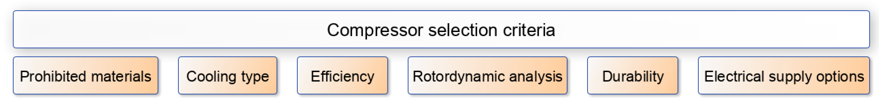
3.2.1. Compressor Preliminary Design and Mass Estimation

Compressors can be divided into displacement type (e.g., sliding vane piston type compressor, mechanical piston compressor) and dynamic type (radial compressor, axial compressor), which possess a rotor equipped with blades, as shown in Figure 8. Displacement compressors are usually used for low volumetric flow rates and relatively high compression ratios, whereas dynamic compressors are more suitable to the current case of higher volumetric flow rates with smaller pressure ratios. Also, it offers design flexibility and low maintenance costs.

The compressor preliminary design includes:

A.

The compressor and motor type selection; and

B.

Sizing and mass estimation of motors and compressors.

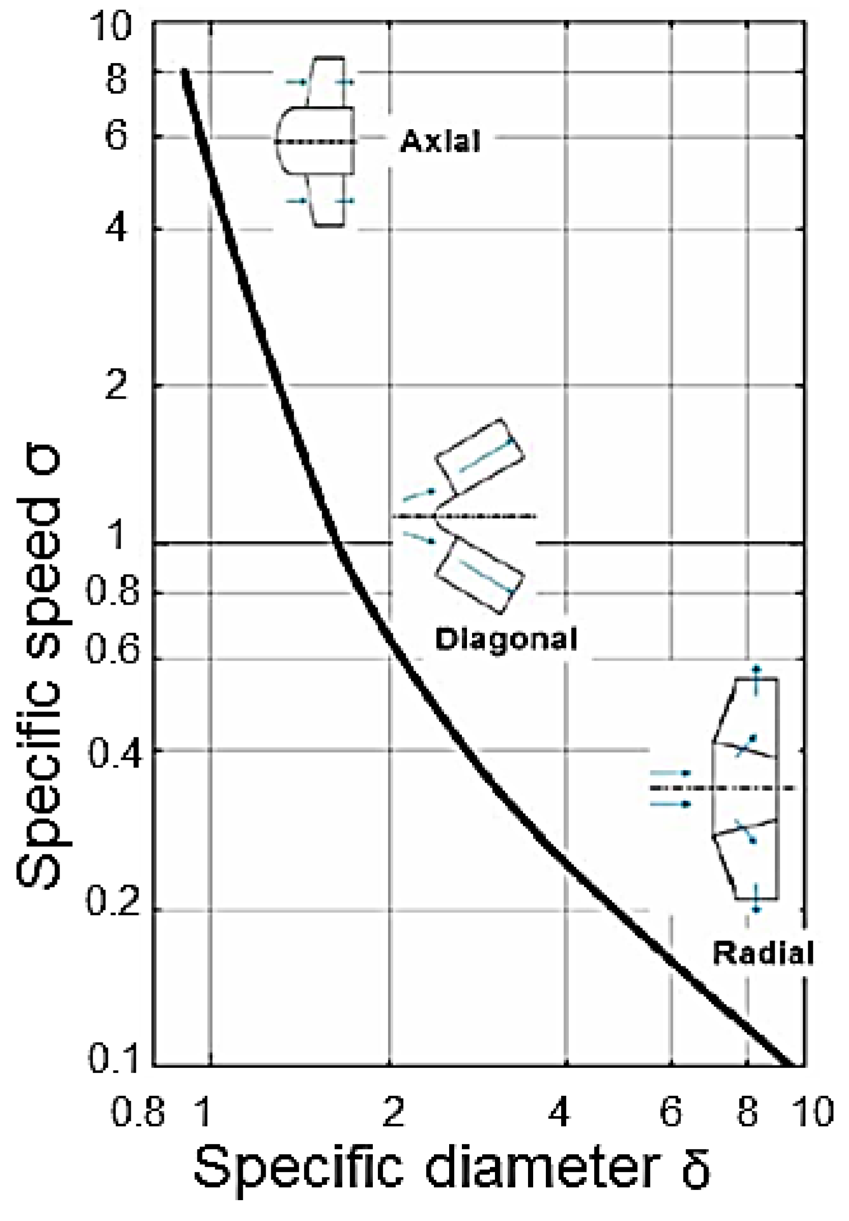
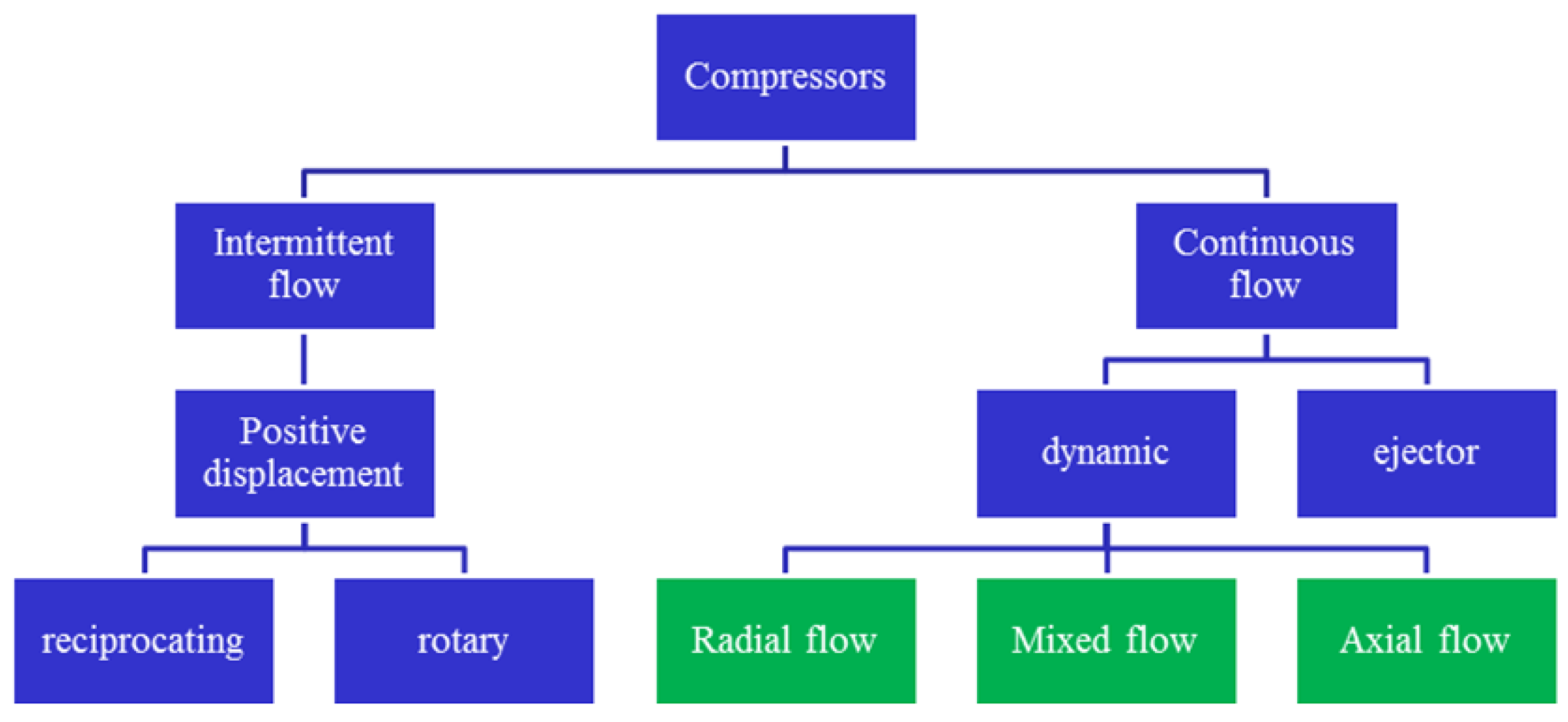
The Compressor and Motor Type Selection

The selection of a dynamic compressor can be performed using a Cordier diagram [16], and the preliminary design can be made once the mass flow $\dot{m}$, the pressure ratio $p_2/p_1$, and the spatial constraints are known. Firstly, using the space constraints from the computer aided design (CAD) model, an initial design diameter d is set, keeping in mind system considerations such as low moment of inertia. Using the initial design diameter, the specific diameter $\delta$ [16] can be calculated using Equation (16).

$$\delta =d·{\left(\frac{2Y_{is}}{{\dot{V}}^2}\right)}^{\frac{1}{4}}·\frac{\sqrt{\pi }}{2}$$

(16)

From the Cordier diagram (Figure 9), the specific speed can be estimated from the calculated specific diameter. The specific speed $\sigma$ is defined as:

$$\sigma =n·\frac{\sqrt{\dot{V}}}{2Y_{is}{}^{\frac{3}{4}}}·2\sqrt{\pi }$$

(17)

where n is the speed in revolutions per second (RPS).

From the obtained specific speed, the type of compressor can be pre-determined. The limits are described below:

• For, 0.8 < $\delta$ < 2; $\sigma$ > 0.8 → Axial compressor is optimal.
• For, 2 < $\delta$ < 4; 0.25 < $\sigma$ < 1 → Diagonal compressor is optimal.
• For, $\delta$ > 4; 0.06 < $\sigma$ < 0.32 → Radial compressor is optimal.

Additionally, it is important to know that the selected compressor satisfies all the important criteria shown in Figure 10.

The compressor’s outer structure must not contain certain materials like gold or magnesium, which are prohibited due to material compatibility, as per manufacturing standards for use in aircraft, which needs to be confirmed by the supplier. Compressor cooling is an important issue and thermal analysis is required to specify the required cooling type. The compressor should possess good efficiency to limit the power off-takes and to have maximum aircraft level benefits, namely drag benefits, reduced fuel consumption, etc. Since some turbo compressors operate at very high speeds (>100,000 RPM), respective stress effects and rotordynamic analysis need to be analyzed in order to eliminate any possible excitation of normal structural modes. High durability is desired for HLFC compressors, as it is necessary to reduce maintenance-related costs and to ensure overall reliability. Finally, to manage installation and spatial constraints, electrical routing and the necessity for additional equipment for compressor operation are key considerations to be addressed.

Sizing and Mass Estimation of Motors and Compressors

The total length of the electric air compressors used for HLFC is the summation of the axial length of the compressor part and the motor. For both axial- and radial-type compressors, a motor space factor $k_m$ = 1.6 is set (which accounts for space occupied by motor electronics/cooling) to conservatively estimate the total effective length of the compressor. Similarly, the mass of the compressor is estimated as the summation of the mass of the individual parts of the compressor.

i.

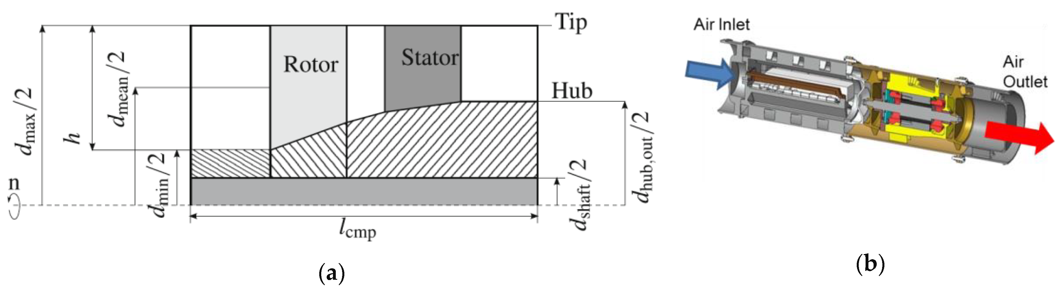
Axial Compressor Sizing and Mass Estimation

In axial compressors, the air flow enters the inlet of the compressor along the axis, and exits it in the same way. It consists of an inlet to take in air, followed by the rotor and stator to achieve compression. The stator acts as a guiding vane for the air to follow the correct axial path and to achieve optimal efficiency. The schematic and cutaway view of an axial compressor is shown in Figure 11a,b, respectively. It consists of a hub as a pathway for the air flow, a shaft connected to the ends of the rotor blade, and a casing to cover the entire compressor, including the electric motor. Hence, the total mass of the axial compressor is the sum of the individual component masses and can be modeled as in Equation (18) [18].

The total mass of an axial compressor is given by the sum of the mass of the axial compressor and the drive (motor) connected to it:

$$m_{axial}=m_{blades}+m_{casing}+m_{shaft}+m_{hub}+m_{motor}$$

(18)

The total length of a single stage axial compressor can be estimated as:

$$l_{axial}=3.25l_{rotor}+l_{stator}+k_m·l_{motor}$$

(19)

The total length for n stage axial compressor can be approximated as:

$$l_{axial}=\left(2+1.25\ast n_{stages}\right)·l_{rotor}+n_{stages}·l_{stator}+k_m·l_{motor}$$

(20)

The detailed algorithm for the preliminary mass and size estimation of axial compressors based on the work of Teichel et.al. [18] and Dixon [19] is given in Appendix B.

ii.

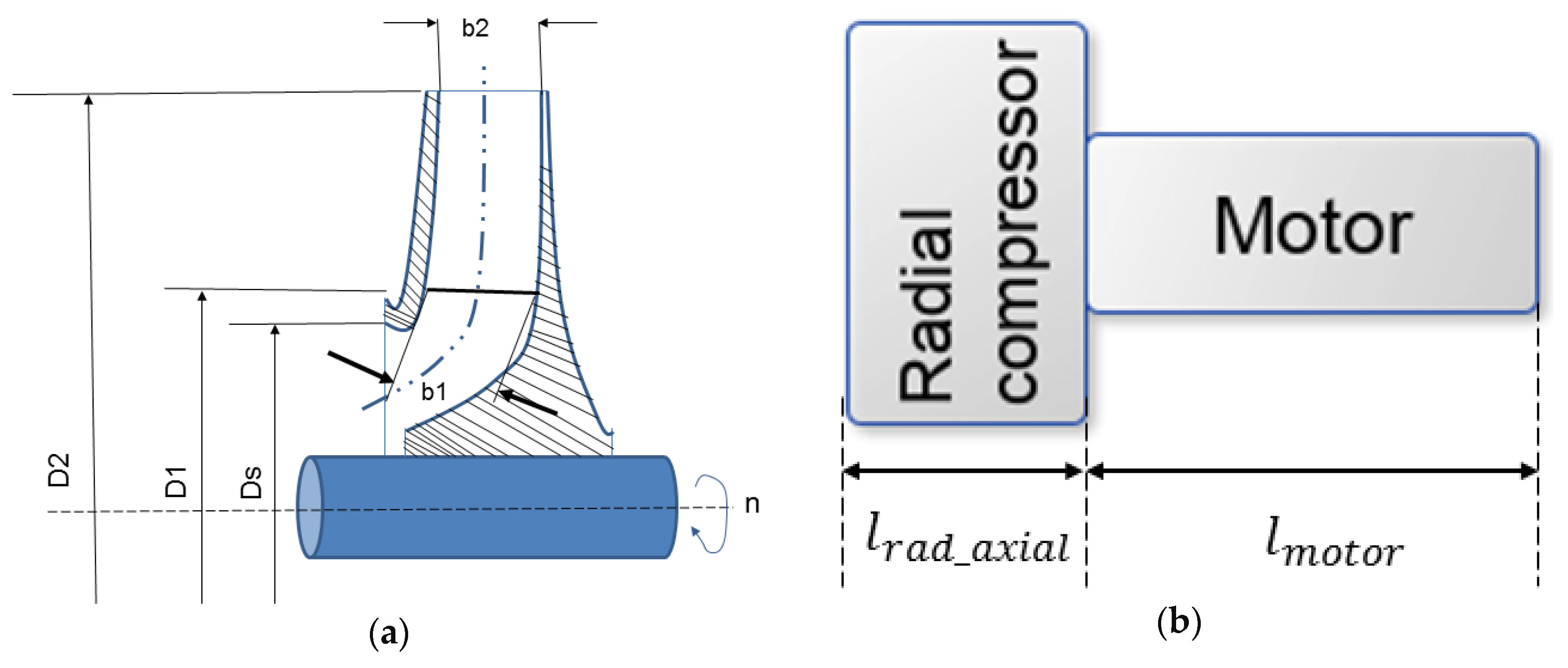
Radial Compressor Size and Mass Estimation

In the case of radial compressors, the airflow enters the impeller inlet along the axis and the compressed air exits perpendicular to that axis. Radial compressors possess a greater stable area of operation in off-design cases than axial compressors. The surge phenomenon, which occurs when lowering the volumetric flow rate and results in an increasing angle of attack at the inlet, is delayed in radial compressors due to the additional acceleration of the flow by cause of the centrifugal forces [20]. Radial compressors possess fewer parts, which makes them cheaper and more robust against dirt and foreign object damage [21]. The impeller meridional view is shown in Figure 12a [22], where D1 is inlet vane diameter, b1 is inlet blade width, D2 is impeller exit diameter, b2 is blade width at the outlet, and Ds is suction diameter.

Much of the mass contribution for the radial compressor is due to the impeller. Hence, the mass of radial compressor coupled with motor can be modeled as in Equation (21).

$$m_{radial}=m_{impeller}+m_{casing}+m_{motor}$$

(21)

The total length of the radial compressor can be estimated as:

$$l_{radial}=k_m·l_{motor}+l_{rad\_axial}$$

(22)

The detailed algorithm for radial compressor sizing and mass estimation is given in Appendix C.

iii.

Motor Selection, Size, and Mass Estimation

A proper motor needs to be selected in order to complete the compressor design process. For low to medium speed (RPM), the induction motor is preferred. However, at high RPM, there are problems, due to slip, for the induction machines. High RPM machines are good in terms of space conservation. Very high RPM feature small compressor diameters which reduce size and mass. These are promising candidates (with further research and adaptation) for HLFC systems in the future. For very high RPM, a permanent magnet synchronous motor (PMSM) is preferred.

In general, from a preliminary design point of view, one can set the limits for drive selection as given below:

• RPM < 50,000–60,000 → Three-phase induction motor.
• RPM > 70,000 → Permanent magnet synchronous motor (PMSM).

The main motor dimensions, the stator core length L, and the stator bore inner diameter $D_{in}$ and outer diameter $D_{out}$ can be calculated using the universal design Equation (23) [23].

$$D_{in}^{2}L=\frac{P\left(kVA\right)}{C_0{N}_s}$$

(23)

where $P\left(kVA\right)$ is the power in kilo volt ampere, given by Equation (24), with the power factor $\cos \varphi$ and $C_0$ given by Equation (25).

$$kVA=\frac{P_{elec}}{\cos \varphi }$$

(24)

$$C_0=1.11\ast {\pi }^2\ast K_w\ast B_{av}\ast A_a\ast {10}^{-3}$$

(25)

$$L=\frac{\pi D_{in}A{R}_{motor}}{2P}$$

(26)

$$D_{out}=\frac{D_{in}}{0.25}$$

(27)

where $A{R}_{motor}$ is the aspect ratio ($L/D_{in}$) of the motor. The approximate motor weight can be estimated conservatively in terms of electrical power (in kW) given by Equation (14) in Section 3.1 as follows:

$$m_{motor}=P\left(\mathrm{kW}\right)/1.2=P_{elec}/1.2$$

(28)

3.2.2. Pneumatic Ducts, Converter, and Electrical Harness Mass Estimation

For a design Mach number inside the duct $M_{duct}$, air density inside the duct ${\rho }_{air}$, the cross-sectional area of duct can be estimated for the duct mass flow rate $\dot{m}$ as

$$A_{cs\_duct}=\frac{\dot{m}}{{\rho }_{air}{M}_{duct}\sqrt{\gamma RT}}$$

(29)

where R is the universal gas constant, and T is the temperature of air inside the duct. $M_{duct}$ of 0.2 is recommended to minimize pressure losses inside the duct. From the calculated cross sectional area of the duct, with thickness t of 2 mm, the duct inner and outer diameter can be determined using Equations (30) and (31), respectively.

$$d_i=2\ast \sqrt{\frac{A_{cs\_duct}}{\pi }}$$

(30)

$$d_0=d_i+t$$

(31)

For a known length $l_{duct}$ and material density ${\rho }_{duct}$ of the duct, the mass of both transfer and exhaust ducts can be estimated as:

$$m_{duct}=\frac{\pi }{4}\ast \left(d_0^2-d_i^2\right)\ast l_{duct}\ast {\rho }_{duct}$$

(32)

The converters, such as variable frequency drive (VFD), for the motors used in the HLFC system depend on the rated power supply and the electrical system architecture. In general, the mass of inverters in term of the total output power is given by [18].

$$m_{inverter}=0.035\frac{\mathrm{kg}}{\mathrm{kW}}$$

(33)

Finally, the mass of electrical harness can be estimated using Equation (34).

$$m_{electric\_harness}=m^{\prime }·P_{elec}·l_{wire}$$

(34)

where $P_{elec}$ is electrical power requirement in kW, $l_{wire}$ is the estimated length of the wire in meters (m), and $m^{\prime }$ is the power specific mass of the wire in (kg/kW-m). The power specific mass can be obtained from the literature using standards like MIL-W-22759/34 [24]. Once the size and mass of the components are estimated, the concept could be further checked in the digital mock-up (Figure 13) for validation of space constraints.

4. Quantitative System Design Case Study with Design Considerations

For the purpose of a quantitative study done as part of the ECHO project, a small leading edge plenum chamber segment of the A350 HTP with a volume of 0.165 m³ was considered, as shown in Figure 14. The design point parameters, such as the plenum pressure, required mass flow rate, temperature, etc., used in the calculations were for 36,000 feet altitude and are shown in

Table 1. Design point parameters for the plenum segment.

Parameters	Estimated Values
Plenum pressure	13,500 Pa
Plenum temperature	240 K
Mass flow requirement	100 g/s

.

The compressor was placed close to the studied plenum segment with negligibly small transfer duct and an exhaust duct of length approximately 0.3 m was used, as shown in the system architecture layout in Figure 15. The arrow marks denotes the direction of airflow.

For the system architecture under design point conditions, the estimated suction power, compressor mass, and sizing parameters using the design approach specified in Section 3 are shown in

Table 2. Estimated design parameters for compressor.

Parameters	Estimated Values
Type	Radial/Mixed flow
Pressure ratio	1.82
Suction power	6 kW
Mass flow	100 g/s
Estimated speed	100,000 RPM
Estimated weight	8 kg
Estimated length	0.21 m

.

The estimated power off-takes and total system mass for the plenum segment were estimated to be 10 kW and 20 kg, respectively. As per the estimated motor parameters that satisfy the HLFC space and mass flow requirements, a 3-phase, 4-pole high-speed PMSM machine was designed using motoranalysis [25], and the permanent magnet material chosen was Recoma 28 Cobalt magnet. The motor parameters are shown in

Table 3. Design parameters for PMSM.

Parameters	Value
Phases	3
Number of poles	4
Number of slots	36
Stator outer diameter (mm)	188
Axial length (mm)	165
Permanent magnet material	Recoma 28 Cobalt

.

The active suction system design is faced with considerable challenges to reach higher technology readiness levels (TRLs). Some of the challenges encountered with possible solutions are presented here, namely the avoidance of water contamination and the thermal management.

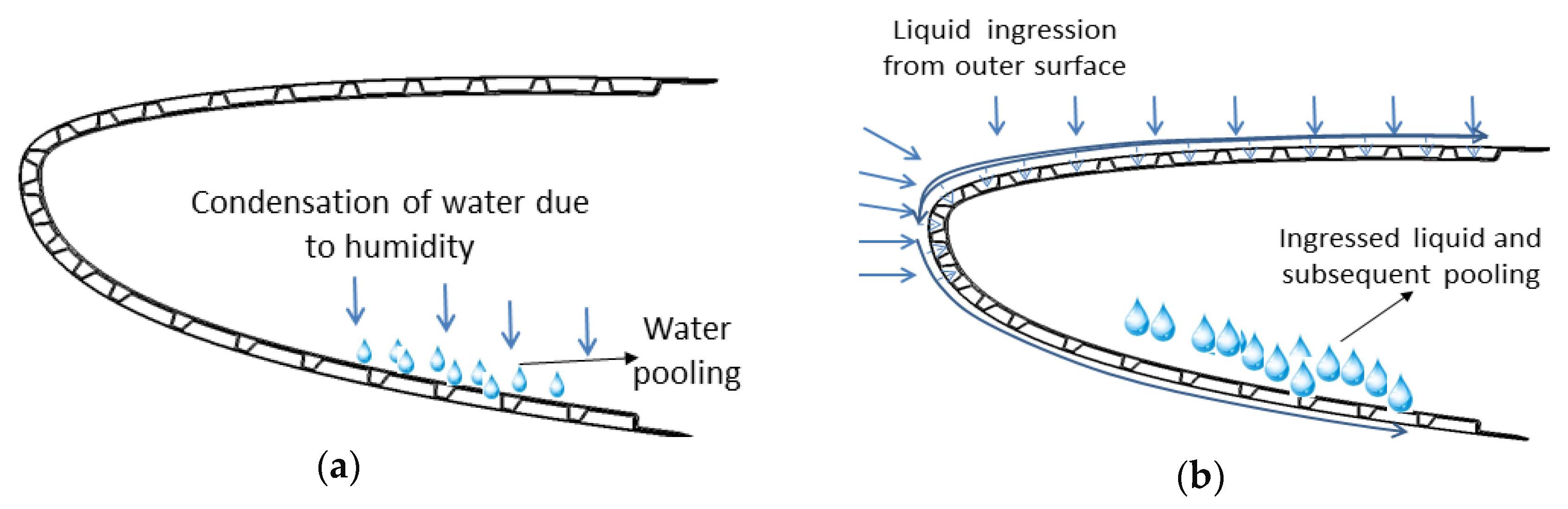
4.1. Water Contamination Avoidance and Its Significance to Suction System Design

Water pooling in the plenum should be avoided and must be drained out before or during take-off to avoid freezing at higher altitudes. The water can get accumulated in the plenum, either due to condensation or water ingress due to rain (Figure 16). It can eventually lead to blockage of pores of the micro-perforated surface. Some possible solutions to tackle this problem are:

• Purging with pressurized air can eliminate pore blockage due to liquid. In purging operation, compressed air is used to unclog the pores. The bleed air for such an operation can be supplied from the engines or through the compressor used for the suction system. The bleed air solution is more challenging due to complexity, mass, and power cost.
• Usage of flapper valves is another possibility to drain water from the plenum. Flapper valves can move liquid from affected segments to non-HLFC segments. However, the complexity of this solution still needs to be assessed.
• The pooled water can be removed by compressor suction and relocated to non-HLFC segments, but this suction will need additional components and add complexity.
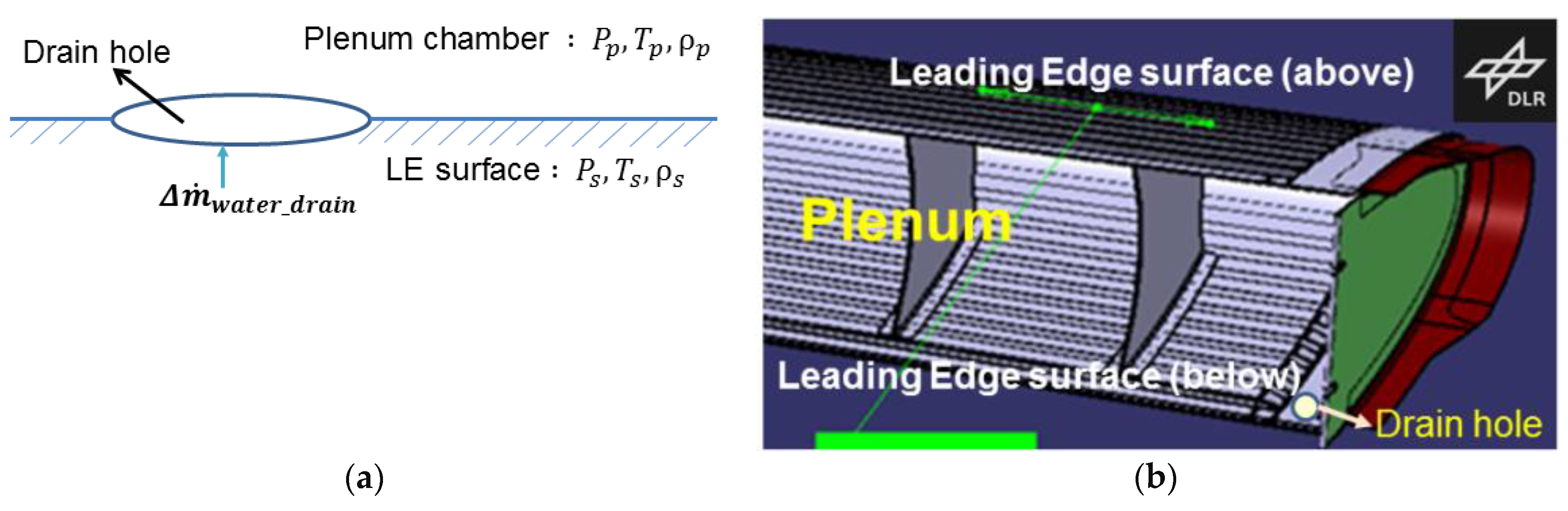
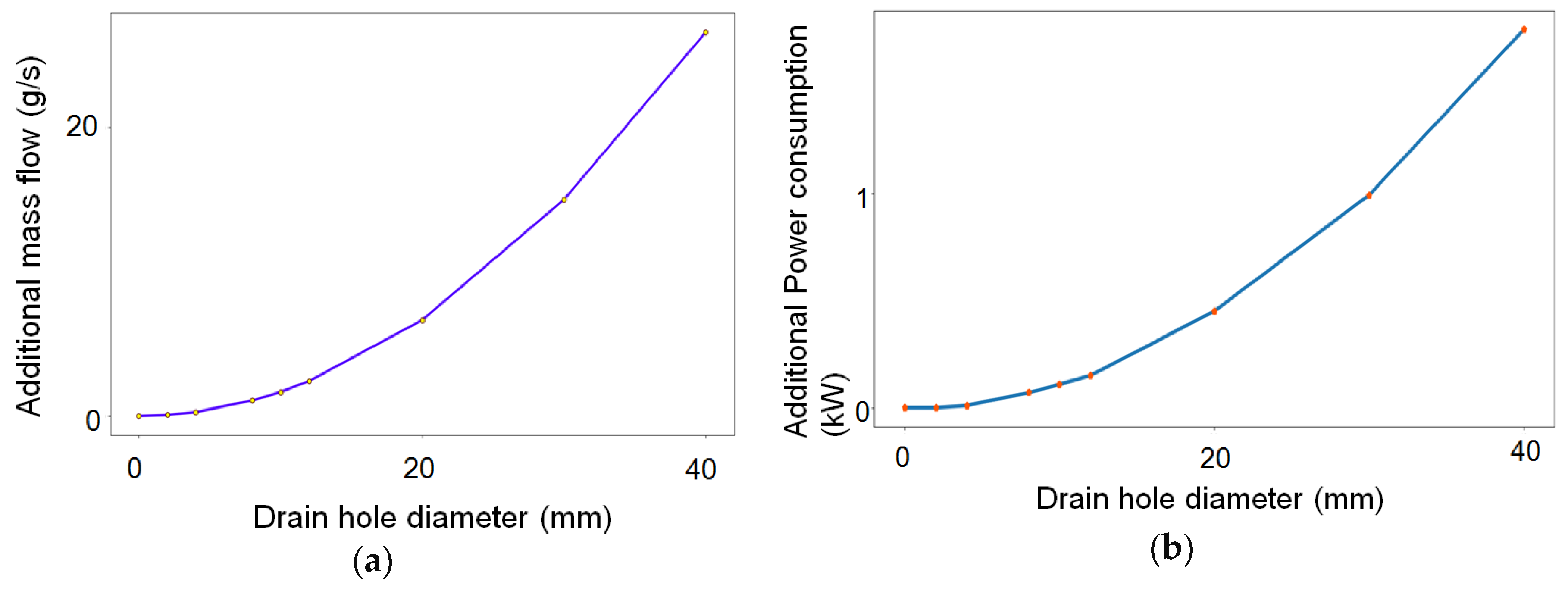
• By using a drain hole in a strategically planned location, the water could be drained out.

4.1.1. Water Amount Estimation

It is important to estimate the amount of water accumulated in the plenum, so as to find a solution for drainage. Condensation takes place when the relative humidity reaches 100%. So, depending on the ground temperature and humidity conditions, the condensation could occur either on ground or within few hundred meters after take-off. The estimation of the amount of water accumulated due to condensation on ground can be made with the classical physics approach by assuming ideal gas laws.

The relative humidity $\varphi$ is the ratio of the actual vapor pressure $P_v$ to the saturated or equilibrium vapor pressure $P_s$.

$$\varphi =\frac{P_v}{P_s}$$

(35)

$$P_{v}V=\varphi P_{s}V=m_w{R}_{w}T$$

(36)

where V is the plenum volume, $R_w$ is the specific gas constant of water with a value of 461.51 J/kg/K, $m_w$ is the mass of water vapor in the plenum, and T is the temperature on ground in Kelvin (K).

The equilibrium water vapor pressure $P_s$ in unit Pascal Pa depends on the temperature and can roughly be estimated using the empiric Magnus-formula in the temperature range of $-{30 }^{°}\mathrm{C}\le T\le {70 }^{°}\mathrm{C}$ [26].

$$P_s=611.213\ast e^{\frac{17.5043T}{241.2+T}}$$

(37)

Here, the unit of temperature T in Equation (37) is degree Celsius (°C). Therefore, for a known volume V, temperature on ground T, and relative humidity $\varphi$ on ground, the mass of water due to condensation is given by

$$m_w=\frac{\varphi P_{s}V}{R_{w}T}$$

(38)

Another possibility for water accumulation is through ingression due to rain $m_{ingress}$. This quantity needs to be determined through experiments and testing, so the total amount of water in the plenum in a worst-case scenario is given by

$$m_{total\_water}=m_w+m_{ingress}$$

(39)

Considering the case study plenum segment with a volume of 0.165 m³, on a hot day with worse humid conditions of 35 °C with relative humidity of 90%, the mass of water that can get accumulated due to condensation can be calculated using Equations (37) and (38).

$$P_s=611.213\ast e^{\frac{17.5043\ast 35}{241.2+35}}=5617\mathrm{Pa}$$

(40)

$$m_w=\frac{p_v·V}{R·T}=\frac{\varphi ·P_s·V}{R·T}=\frac{0.9·5617\mathrm{Pa}·0.165{\mathrm{m}}^3}{461.51\frac{\mathrm{J}}{\mathrm{K}\mathrm{g}·\mathrm{K}}·308.15\mathrm{K}}=0.0059\mathrm{kg}$$

(41)

Hence, for the given plenum volume, the accumulated water due to condensation could be 5.9 g, which is very miniscule, and the drain hole solution could be simple and well suitable for the present case. However, the amount of water accumulated due to condensation increases with the volume of the plenum considered. Furthermore, there could be additional accumulation of water possible due to rain or other factors. It is advised to test with coupons to determine how much water can enter through the micro-perforations over a given period of time under rainy conditions.

4.1.2. Water Drain Hole Effects Analysis

One way of eliminating the water in the plenum is with the help of an open drain hole, placed in the area where water pooling is more likely. This solution could be feasible for HTP and wing areas, for the VTP gravity helps in draining out accumulated water.

A negative effect of the drain hole during cruise is the additional air mass flow $\Delta {\dot{m}}_{water\_drain}$ (see Figure 17a) due to air leakage, created during HLFC system operation as a result of the differential pressure between the leading edge (LE) surface and the plenum. This additional mass flow can be calculated as follows:

$$\Delta {\dot{m}}_{water\_drain}=\sqrt{\frac{\gamma }{\gamma -1}\frac{2}{R}}{A}_0{C}_d\frac{P_s}{\sqrt{T_s}}\sqrt{{\left(\frac{P_p}{P_s}\right)}^{2/\gamma }-{\left(\frac{P_p}{P_s}\right)}^{\left(\gamma +1\right)/\gamma }}$$

(42)

where $P_p$ is the plenum pressure, $T_s$ is the surface temperature, $P_s$ is the surface pressure close to the drain hole, $A_0$ is the hole area, $C_d$ is the discharge coefficient, R is the specific gas constant for air, and γ is the ratio of specific heats.

For the preliminary design of the compressor, the two important parameters are the mass flow rate and the pressure ratio. As seen earlier, the mass flow in the plenum ${\dot{m}}_{plenum}$ is the calculation result from the aerodynamics domain. However, the final total mass flow rate for the compressor also depends on other factors, namely the mass flow increase due to the water drainage solution $\Delta {\dot{m}}_{water\_drain}$ and the increased or decreased mass flow rate due to chamber optimization $\Delta {\dot{m}}_{chamber\_opt}$. In addition, there will be further mass flow value changes due to uncertainties such as manufacturing tolerances, surface imperfections, etc. that may arise. To account for this, a third term $\Delta {\dot{m}}_{uncertainity}$ is introduced in Equation (43), which can be approximated as given in Equation (44) where a factor of safety (FS) of 2 is introduced to have a more optimistic mass flow value. Hence, the total optimized mass flow at the compressor inlet is given by Equation (43).

$${\dot{m}}_{total}={\dot{m}}_{plenum}+\Delta {\dot{m}}_{water\_drain}\pm \Delta {\dot{m}}_{chamber\_opt}+\Delta {\dot{m}}_{uncertainity}$$

(43)

$$\Delta {\dot{m}}_{uncertainity}=FS\ast \max \left(\Delta {\dot{m}}_{wate{r}_{drain}},\Delta {\dot{m}}_{chamber\_opt}\right)$$

(44)

The above equations hint to the fact that the HLFC suction system design is interlinked with many disciplines and subsystems, the final mass flow depends on the system solution chosen for water drainage, and the aerodynamic structures optimization on chamber design.

For a drain hole located on the lower surface of the leading edge (in the studied plenum segment), a sensitivity study was conducted to see the effect of the hole diameter on the mass flow influx and on the suction power increment due to the added mass flow.

For a chosen leading edge surface pressure of 16,000 Pa and a plenum pressure at design flight point (36.000 feet), the results can be seen in Figure 18. As the drain hole diameter increases, there is large influx of additional mass flow; this increases the work load of the compressor, and hence, the system suction power requirement increases considerably. In order to minimize mass flow influx, a drain hole diameter of up to 8–10 mm could be considered, so that a large change in power consumption could be avoided. Testing of the drain hole solution to check for effective draining of water from the plenum is necessary in order to compare it with other solutions for drainage.

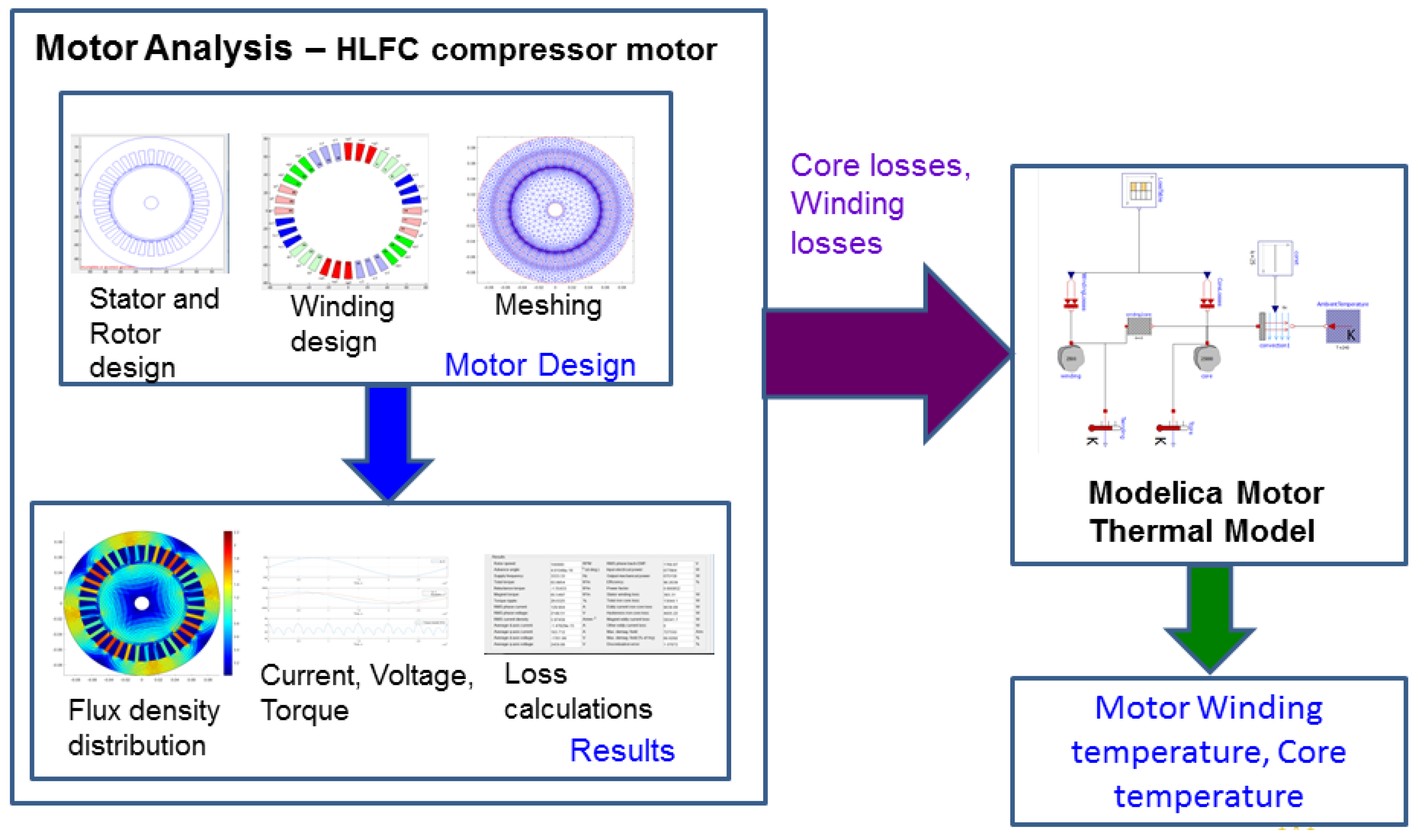
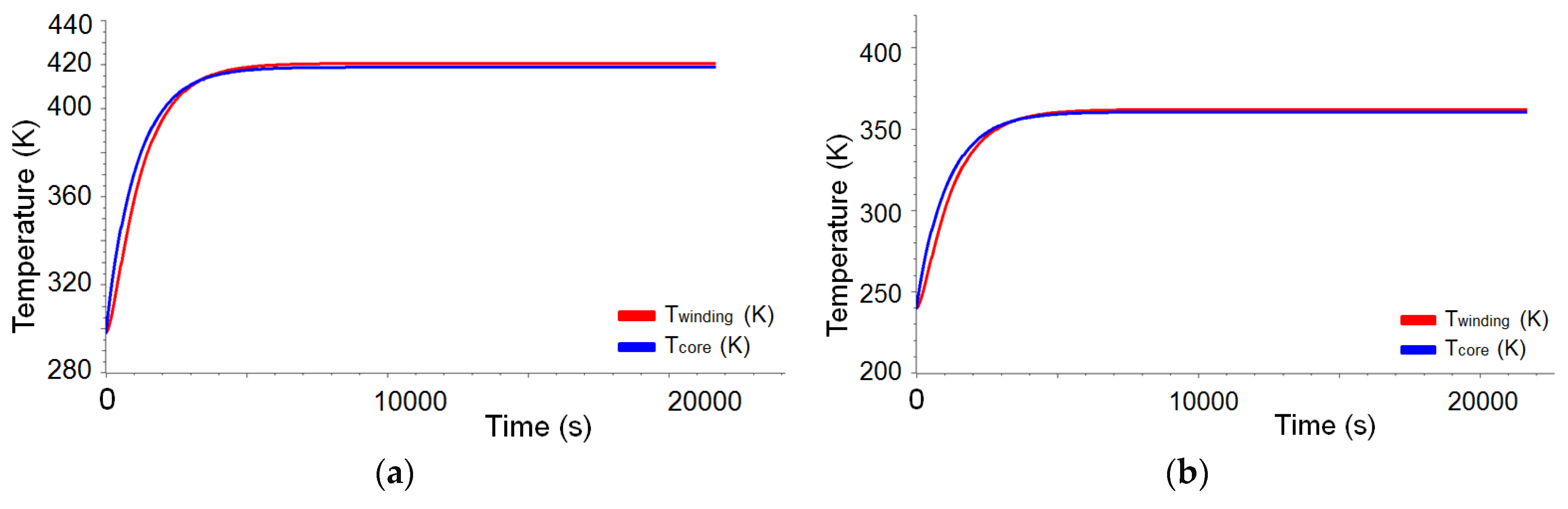
4.2. Thermal Management of Motor

The compressor and the associated power electronic components are expected to overheat when operated for a longer duration, and hence, proper thermal management is necessary. The alternating current (AC) motor driving the suction system compressor is bound to overheat. It consists of two parts, namely the stationary part called the stator and the rotational part called the rotor. For the motor, the losses generated are dissipated into heat, and the two main losses concerning the electrical machine are:

• Copper loss or winding loss $P_{Cu}$: This loss is caused by the winding resistance. In general, it can be mathematically expressed as $i^2.R\left(T_1\right)$, where i is the rated current and R($T_1$) is the winding resistance at temperature measured at temperature $T_1$.
• Iron core loss $P_{Fe}$: This loss occurs in the magnetic material of the motor and consists of two types:

  ○

  Eddy current loss: In the alternating current (AC) machines, currents get induced in the stator due to the rotating magnetic field according to Faraday’s law, and this induced current (also called eddy currents) dissipates into heat [27].

  ○

  Hysteresis loss: This loss occurs due to the interaction of the changing magnetic fields with the stator iron core, which is subjected to magnetization and demagnetization.

Currently, research is being made in reducing machine losses, which contribute to heat generation and also to the cooling aspects [28,29]. In order to study the temperature rise in the windings and core, a low order thermal analysis method, as shown in Figure 19, was used.

Initially, a motor was designed using the software called motoranalysis [25], which allows to select the stator and rotor diameter, the length, the number of slots, and the type of winding used. Once the stator and the rotor were designed, mesh could be generated in the windings and in the air-gap for performing a magnetostatic analysis. The results obtained after the magnetostatic analysis include the flux density distribution in the windings and the air-gap, the current and voltage distribution, the torque, and the generated losses.

The generated loss values were used in the lower order Modelica thermal model. Since the HLFC is supposed to operate continuously in cruise, both the winding and core loss values were fed to the heat flow component in Modelica during the desired time duration. The winding losses were corrected according to the temperature. The heat dissipation to the environment was modeled as the thermal conductance between the windings and the core, heat storage in windings, as well as core as a heat/thermal capacitor element and convection due to the external environment (due to prevailing ambient temperature). The intention of the performed study was to see the temperature rise in the core and windings for long duration operation in given ambient conditions. The value of the thermal capacitances for the winding and the core were computed based on the steady state thermal network [30] and the datasheet thermal resistance values for industrial electric motors [31].

A thermal analysis was performed for the compressor designed for the studied plenum segment. The PMSM machine was analyzed for 100,000 RPM for both ground operation and high altitude operation, and the results are shown in Figure 20a,b, respectively.

The supply (rated) current to the motor was chosen from the datasheet [32] provided by commercial turbo-compressor suppliers. The current supply was limited and a high voltage was supplied through an inverter. This led to a decrease in copper loss in the stator windings, but due to high RPM, the core loss increased considerably. For ground operations, an ambient temperature of 298 K was assumed and for high altitude operation, ambient temperature of 240 K was assumed for simulation. Since the HLFC system operates for longer duration continuously during cruise, the simulation time was set to 6 h or 21,600 s, and the core and winding temperature rise was measured.

It can be seen from the study that, in ground operation, the temperature exceeds 400 K (125 °C), while for high altitudes operation, the ambient temperature helps in cooling of the motor, but still has the potential to exceed 360 K. It can be concluded that for very high RPM machines, the temperature rise will be very high and to prevent overheating of windings, a proper cooling arrangement such as forced convection or liquid-based cooling needs to be considered. Also, the overheating of the core will cause demagnetization of the permanent magnet (PM), hence a proper core with high Curie temperatures [33] should be chosen for electrical machine design for HLFC compressors.

Additionally, the viscous friction in the air-gap between the stator and rotor increases considerably at high speeds, and there is a potential for heat generation due to high rotation in compressor parts as well; hence, these aspects needs to be considered for future study. A complete multi-physics analysis using finite element method (FEM) is suggested for compressor designers in order to model the complete thermal behavior of the compressors during HLFC operation.

5. Discussion and Conclusions

This paper presented a generalized approach for the preliminary design of an HLFC system intended for conceptual studies. The method can be applied for evaluation of different HLFC system architectures and for concept feasibility checks. The compressor design approach gives mass and dimensions as outputs with good approximations. However, the final estimated values also depend on the material chosen for various parts of the compressors. It is advised to refer to the current trends in the industry for proper material selection, so that the error margin is minimal.

This paper also discussed the various challenges associated with the HLFC system design in Section 4, which need to be considered for a preliminary design and also for overall system development. The important points to be considered in the HLFC suction system design and from the various studies conducted are summarized below:

• While assessing the concepts, it is also important to consider solutions for other system issues, such as water drain from the plenum and optimized chamber layout for suction in the leading edge. These aspects result in additional mass flow into the plenum, hence the compressor preliminary design process should consider these issues as well. A simple drain hole solution is proposed in the paper; however, to check for the effectiveness of this solution, it should be tested in a ground-based demonstrator.
• Thermal management and fire protection of the suction system components is an important safety and certification requirement, and hence need to be considered in the early stages of system development. Proper cooling solutions need to be identified for the HLFC system components. It is advisable to perform multi-physics thermal simulation of the compressor and to test the complete HLFC suction system in a demonstrator in simulated flight conditions to check for functionality and effectiveness of the proposed cooling solution.

The following points need to be considered for evaluation of HLFC concepts:

• The exact location of the compressor exhaust in the aircraft should be known prior to concept assessment. Based on the location, the outflow pressure will be different and cause considerable changes in mass and power consumption. The location should be optimized in synergy with other involved disciplines. It is suggested that the location of the exhaust should be chosen so as to not cause any considerable flow changes over the airfoil, and the blow from the exhaust should not induce a humid atmosphere in the vicinity and affect nearby systems.
• The design of an HLFC system on a wing should be performed in coordination with the wing ice protection system (WIPS) and structural design, so that the optimal location for suction system concepts and the compressor exhaust can be allocated.
• All potential concepts should be simultaneously checked in the digital mock-up to ascertain if it is feasible in the early stages. This saves developmental costs. It is also necessary to consider the manufacturing feasibility of the proposed concept, and the same should be discussed with the suppliers.

The HLFC system design calls for many innovations to improve the overall technology readiness levels (TRL) of the system. Some future research aspects are proposed:

• High efficient compressors are required for HLFC, especially in low Reynolds number flows, since they are operated at very high altitudes.
• The motor needs to be durable and should not get overheated, and require simple, innovative, and cost-effective cooling solutions.
• The PMSM motors need to use quality permanent magnets with high Curie temperature, with less probability for demagnetization; hence, proper materials need to be selected and researched for such magnets to be used for HLFC applications.

References

- Krishnan, K.S.G.; Bertram, O.; Seibel, O. Review of hybrid laminar flow control systems. Prog. Aerosp. Sci. 2017, 93, 24–52. [Google Scholar] [CrossRef]
- Robert, J.P. Drag Reduction: An Industrial Challenge; Agard Report 786 Special Course on Skin Friction Drag Reduction: Neuilly Sur Seine; Airbus Industrie Blagnac: Blagnac, France, 1992. [Google Scholar]
- Joslin, R.D. Overview of Laminar Flow Control; NASA/TP-1998-208705; NASA: Hampton, VA, USA, 1998.
- Young, T.M. Investigations into the Operational Effectiveness of Hybrid Laminar Flow Control Aircraft. Ph.D. Thesis, School of Engineering, Cranfield University, Cranfield, UK, 2002. [Google Scholar]
- Boeing Inc. Hybrid Laminar Flow Control Study Final Technical Report; NASA Contractor Report 165930; NASA: Hampton, VA, USA, 1982.
- Schrauf, G.; Horstmann, K.H. Simplified Hybrid Laminar Flow Control. In Proceedings of the European Congress on Computational Methods on Applied Sciences and Engineering (ECCOMAS 2004), Jyväskylä, Finland, 24–28 July 2004. [Google Scholar]
- Krishnan, K.S.G.; Bertram, O. Assessment of a Chamberless Active Hybrid Laminar Flow Control System for the Vertical Tail Plane of a Mid-Range Transport Aircraft. In Proceedings of the Deutscher Luft- und Raumfahrtkongress (DLRK 2017), Munich, Germany, 5–7 September 2017. [Google Scholar]
- Jabbal, M.; Everett, S.; Krishnan, K.S.G.; Raghu, S. A Comparative Study of Hybrid Flow Control System Architectures for an A320 Aircraft. In Proceedings of the 8th AIAA Flow Control Conference, AIAA AVIATION Forum, (AIAA 2016-3928), Washington, DC, USA, 13–17 June 2016. [Google Scholar]
- Pe, T.; Thielecke, F. Synthesis and Topology Study of HLFC System Architectures in Preliminary Aircraft Design. In Proceedings of the 3rd CEAS Air&Space Conference, Venice, Italy, 24–28 October 2011; pp. 1460–1471. [Google Scholar]
- Pe, T.; Thielecke, F. Methodik zur Leistungsabschätzung von HLFC-Absaugsystemen im Flugzeugvorentwurf. In Proceedings of the Deutscher Luft- und Raumfahrtkongress (DLRK), Hamburg, Germany, 31 August–2 September 2010. [Google Scholar]
- RTCA/DO-160G. Environmental Conditions and Test Procedures for Airborne Equipment; Section 8, Vibrations; RTCA, Inc.: Washington, DC, USA, 2010. [Google Scholar]
- Henke, R. A320 HLF Fin Flight Tests Completed. Air Space 1999, 1, 76–79. [Google Scholar] [CrossRef]
- Idelchik, I.E. Handbook of Hydraulic Resistance, 3rd ed.; CRC Press: Boca Raton, FL, USA, 1996. [Google Scholar]
- Bohl, W.; Elmendorf, W. Strömungsmaschinen 1—Aufbau und Wirkweise; Vogel Business Media: Würzburg, Germany, 2013. [Google Scholar]
- Bornholdt, R.; Pe, T.; Thielecke, F. Modellierung und Simulation eines Absaugsystems für ein Seitenleitwerk mit hybrider Laminarisierung. In Proceedings of the Deutscher Luft- und Raumfahrtkongress (DLRK), Hamburg, Germany, 31 August–2 September 2010. [Google Scholar]
- Cordier, O. Ähnlichkeitsbedingungen für Strömungsmaschinen; Brennstoff, Wärme, Kraft (BWK): Düsseldorf, Germany, 1953; Volume 5, pp. 337–340. [Google Scholar]
- Epple, P.; Durst, F.; Delgado, A. A theoretical derivation of the Cordier diagram for turbomachines. Proc. Inst. Mech. Eng. Part C J. Mech. Eng. Sci. 2011, 225, 354. [Google Scholar] [CrossRef]
- Teichel, S.H.; Dörbaum, M.; Misir, O.; Merkert, A.; Mertens, A.; Seume, J.R.; Ponick, B. Design considerations for the components of electrically powered active high-lift systems in civil aircraft. CEAS Aeronaut. J. 2015, 6, 49–67. [Google Scholar] [CrossRef]
- Dixon, S.L.; Hall, C.A. Fluid Mechanics and Thermodynamics of Turbomachinery; Butterworth-Heinemann/Elsevier: Amsterdam, The Netherlands, 2010. [Google Scholar]
- Menny, K. Strömungsmaschinen: Hydraulische und Thermische Kraft- und Arbeitsmaschinen; B.G. Teubner Verlag: Wiesbaden, Germany, 2006. [Google Scholar]
- Andrich, B. Flugzeugstrahltriebwerke; Lecture Notes; Hamburg University of Technology: Hamburg, Germany, 2012. [Google Scholar]
- Wulff, D.; Kosyna, G. HIGHER-LE Workshop “Auslegung von Radialverdichtern”; Technische Universität Braunschweig: Braunschweig, Germany, 2009. [Google Scholar]
- Müller, G.; Vogt, K.; Ponick, B. Berechnung Elektrischer Maschinen; Wiley-VCH: New York, NY, USA, 2008. [Google Scholar]
- Wiremasters. Available online: https://www.wiremasters.net/products/grid?category=m22759-34 (accessed on 13 August 2019).
- Motoranalysis. Available online: http://motoranalysis.com/ (accessed on 13 August 2019).
- Hakenesch, P.R. Technische Thermodynamik; Lecture Notes; Version 2.1; Munich University of Applied Sciences: Munich, Germany, 2010. [Google Scholar]
- Sarma, M. Electric Machines: Steady-State Theory and Dynamic Performance, 2nd ed.; West Publishing Company: St. Paul, MN, USA, 1994. [Google Scholar]
- Hong, D.K.; Woo, B.-C.; Lee, J.Y.; Koo, D.H. Ultra high speed motor supported by air foil bearings for air blower cooling fuel cells. IEEE Trans. Magn. 2012, 48, 871–874. [Google Scholar] [CrossRef]
- Tosetti, M.; Maggiore, P.; Cavagnino, A.; Vaschetto, S. Conjugate heat transfer analysis of integrated brushless generators for more electric engines. In Proceedings of the 2013 IEEE Energy Conversion Congress and Exposition, Denver, CO, USA, 15–19 September 2013; pp. 1518–1525. [Google Scholar] [CrossRef]
- Rajput, N.M. Thermal Modeling of PMSM and Inverter. Master’s Thesis, Georgia Institute of Technology, Atlanta, GA, USA, May 2016. [Google Scholar]
- Parker Hannafin Corporation, GVM210-150P6 Datasheet. Available online: https://www.parker.com/parkerimages/Market-Tech/Market-Tech%20Home/Hybrid%20Electric%20Vehicles/Literature/GVM210-050%20Brochure.pdf (accessed on 13 August 2019).
- Datasheet for EMTC 120k Compressor; Fischer Spindle: Herzogenbuchsee, Switzerland, 2019.
- Bianchi, N.; Bolognani, S.; Luise, F. Potentials and limits of highspeed PM motors. IEEE Trans. Ind. Appl. 2004, 40, 1570–1578. [Google Scholar] [CrossRef]