Multi-Disciplinary Design Optimisation of the Cooled Squealer Tip for High Pressure Turbines

Abstract
:
1. Introduction
2. Optimisation Strategy
2.1. Multipoint Approximation Method
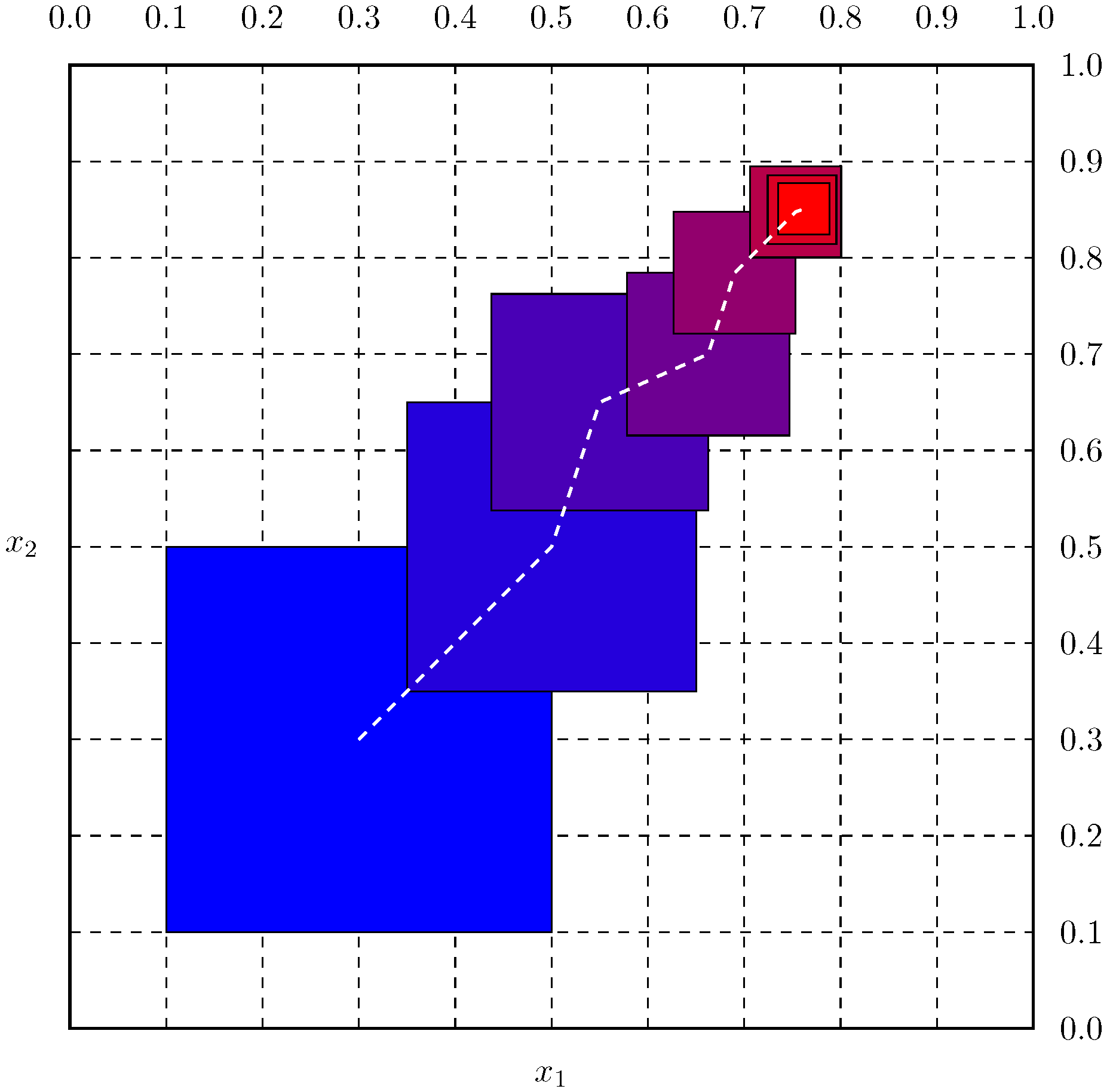
- Initialization: choose a starting point and initial trust region such that .In practice, the initial subregion is a box centred at .
- At the k-th iteration, the current approximation to the constrained minimum is , and the current trust region is .
- (a)
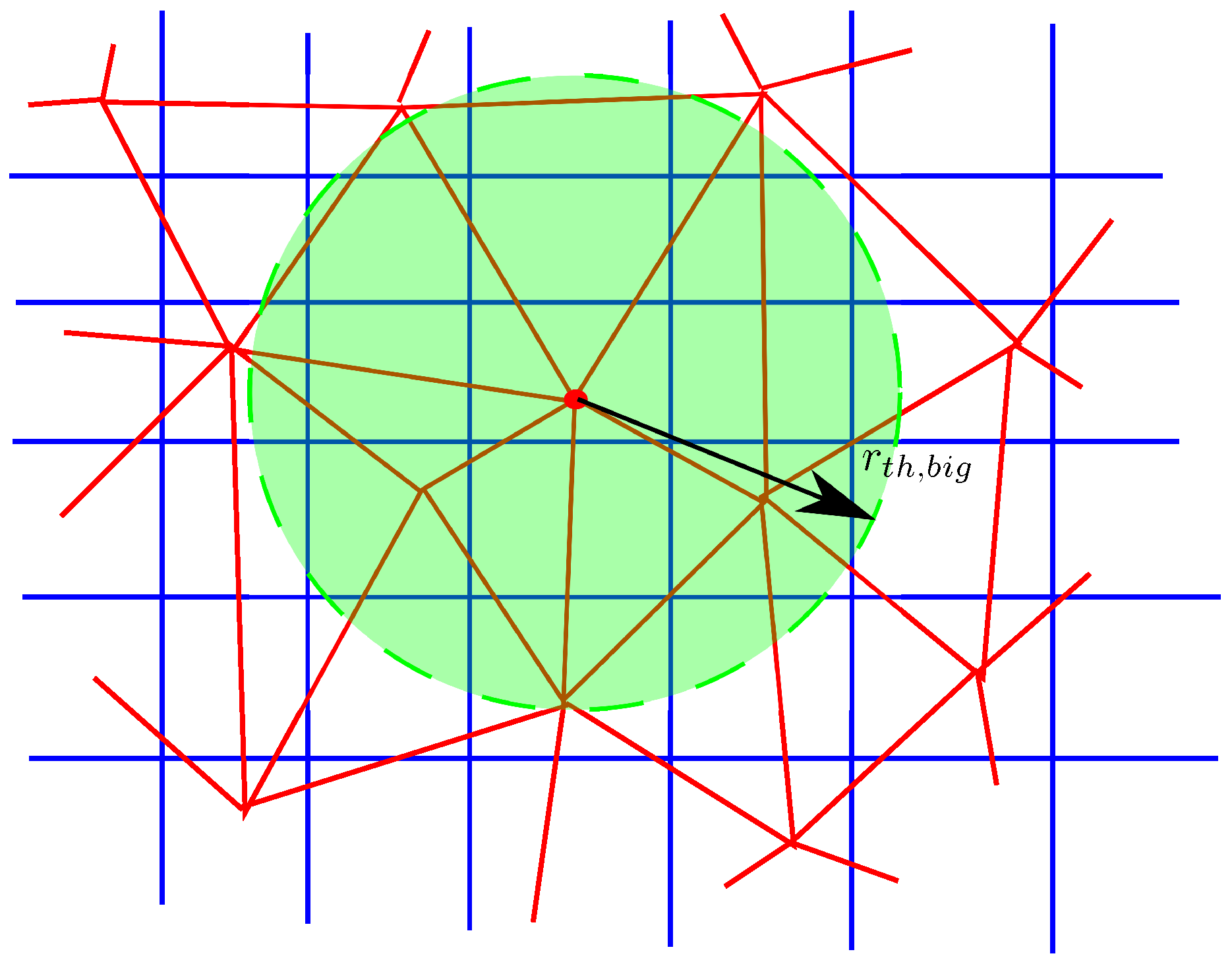
- Choose a set of points that will be used to build approximations. This procedure is often referred to as the Design of Experiments (DoE).
- (b)
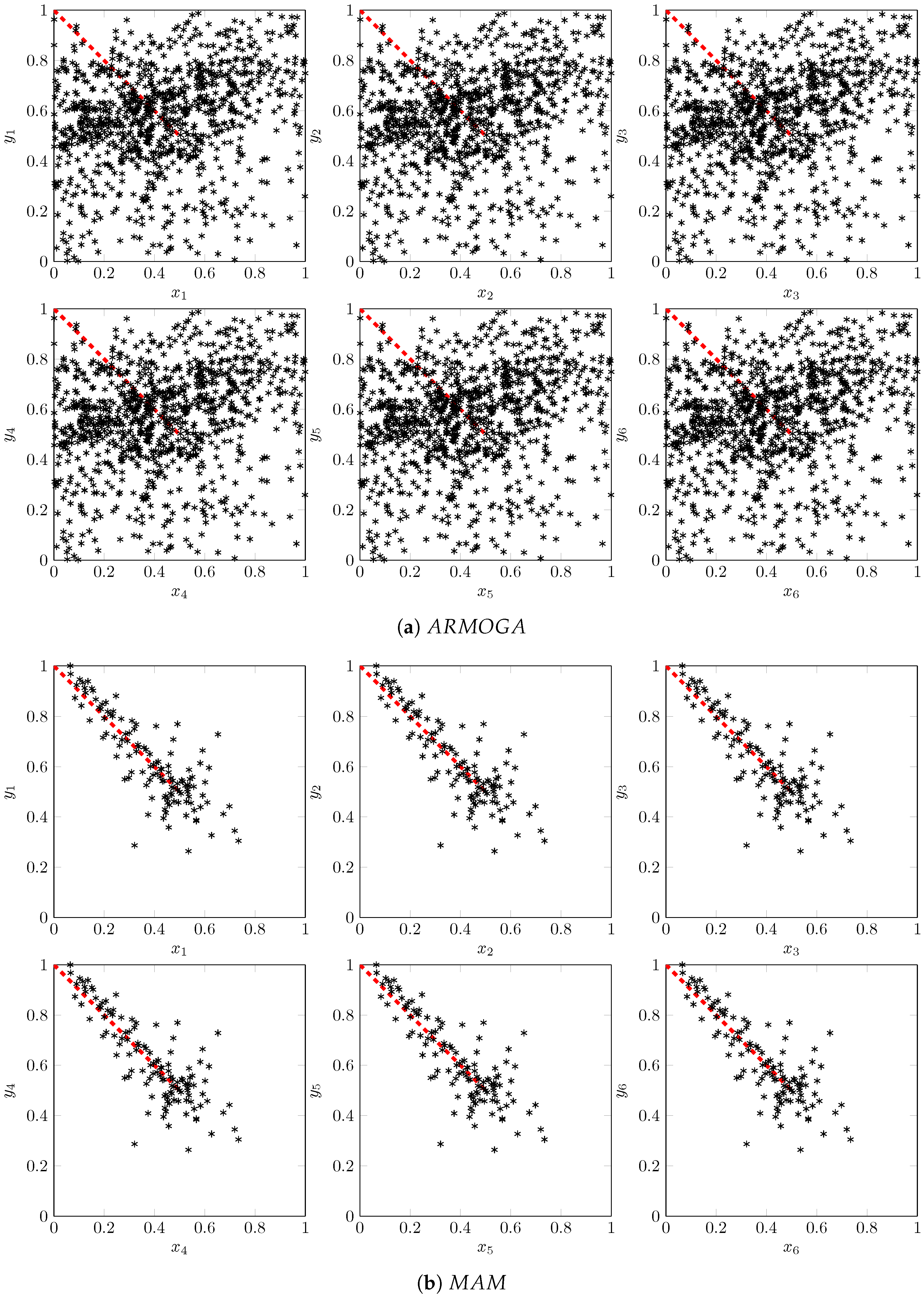
- Build approximations using any suitable method. Two approximation techniques are currently implemented in the MAM: the Metamodel Assembly [15] and the Moving Least Squares Method [16].Denote the approximate objective function and constraints by and , , respectively.
- (c)
- Replace the original optimization problem (Equation (1) by the following one:Find the next approximation to the optimal point, solving the approximate problem (Equation (2)).
- (d)
- Terminate optimization. The obtained approximation to the solution of problem (Equation (1)) is .
2.2. Multi-Objective Problem Formulation
2.3. Bound Formulation of Minmax Problems
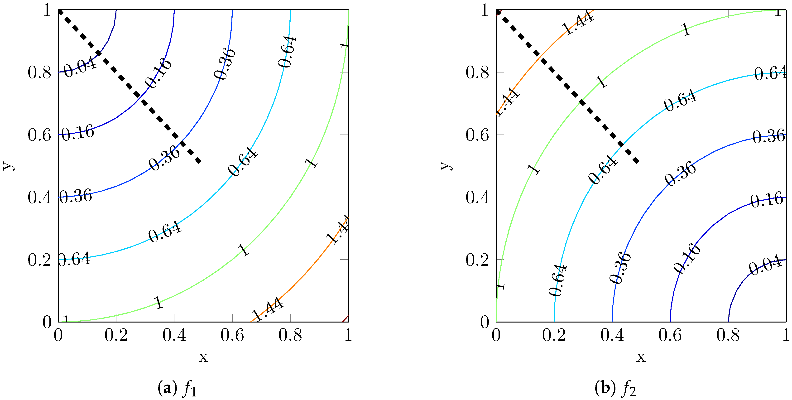
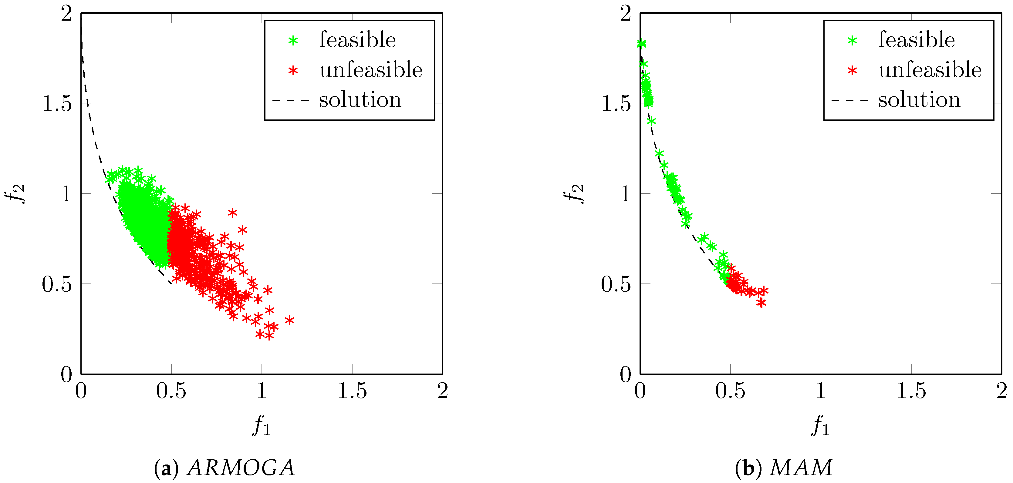
2.4. Analitycal Verification
3. Application
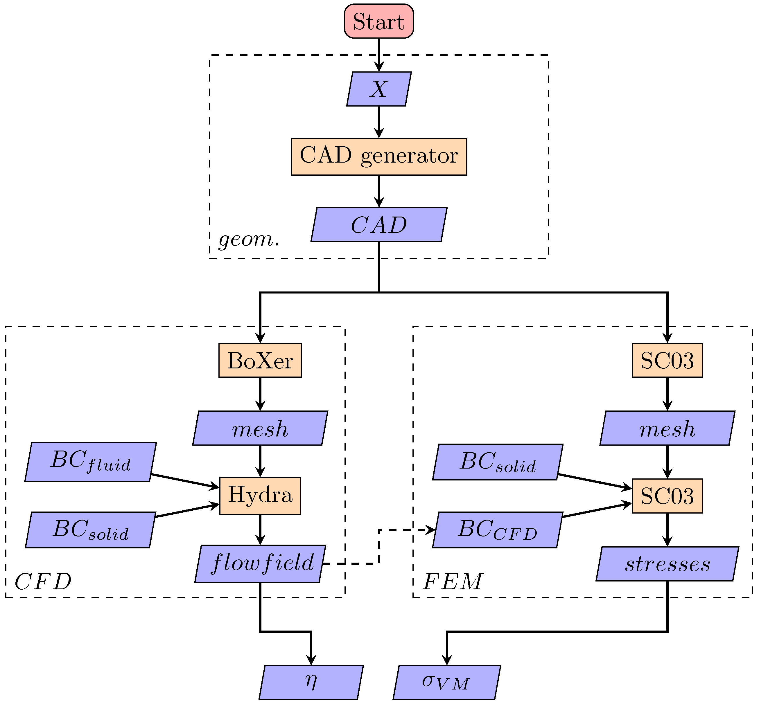
3.1. Simulation Workflow and Objectives
- The Geometry Creation (),
- The Thermal-fluid analysis (),
- The Structural analysis ().
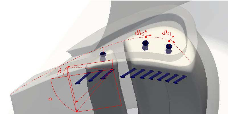
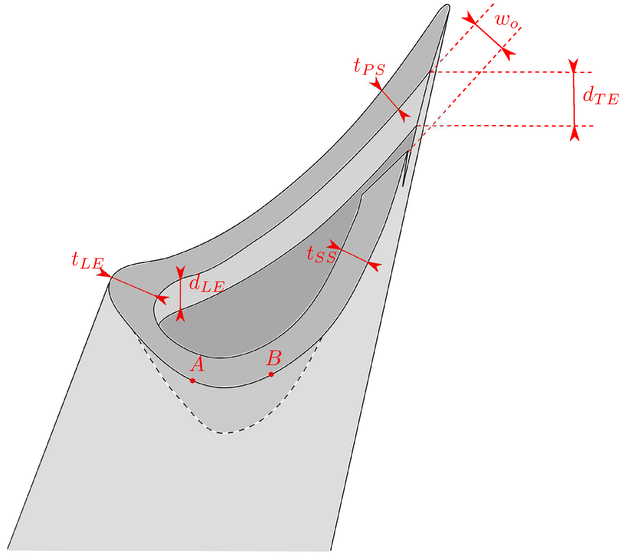
3.1.1. Geometry
Tip Design
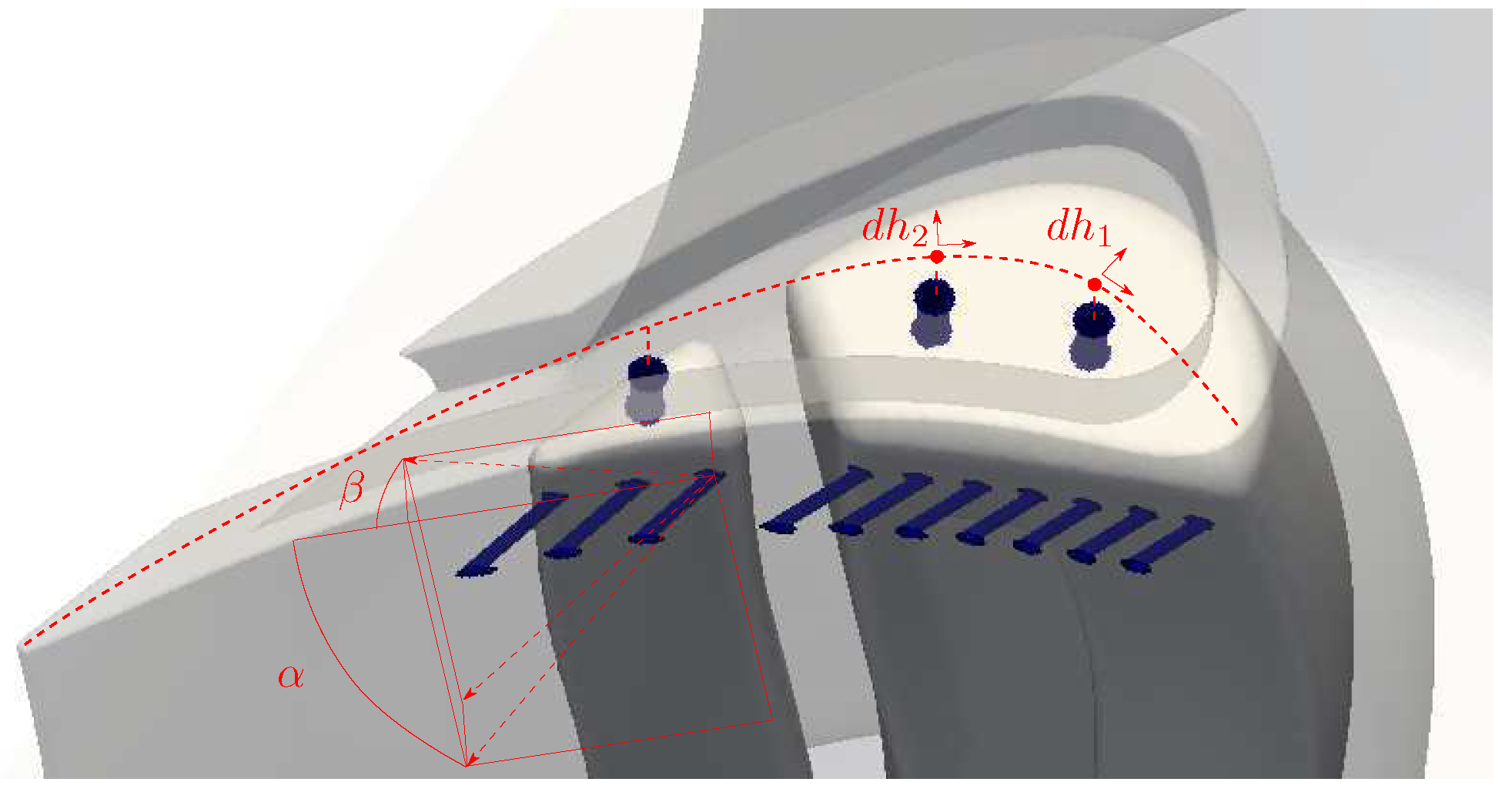
Internal Cooling System
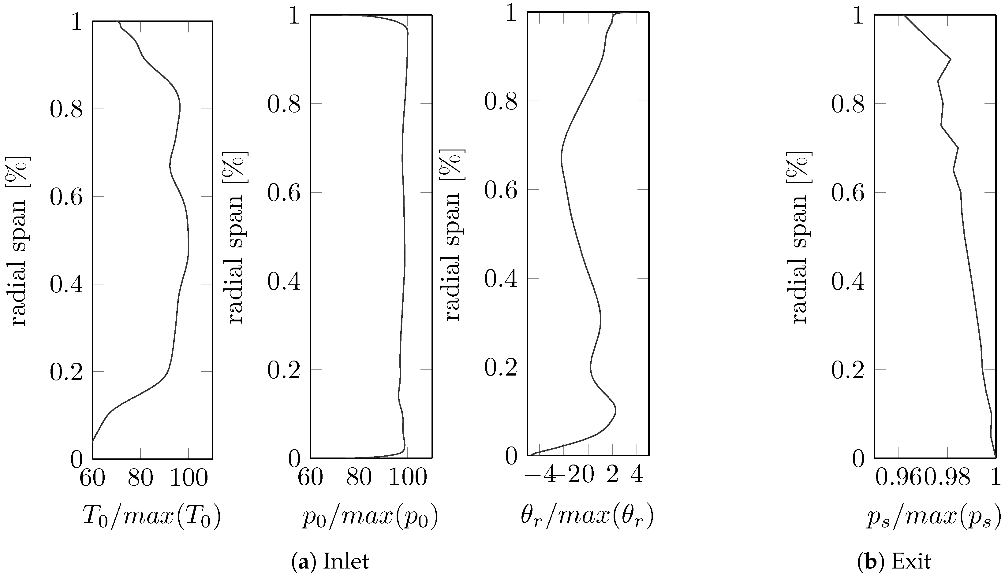
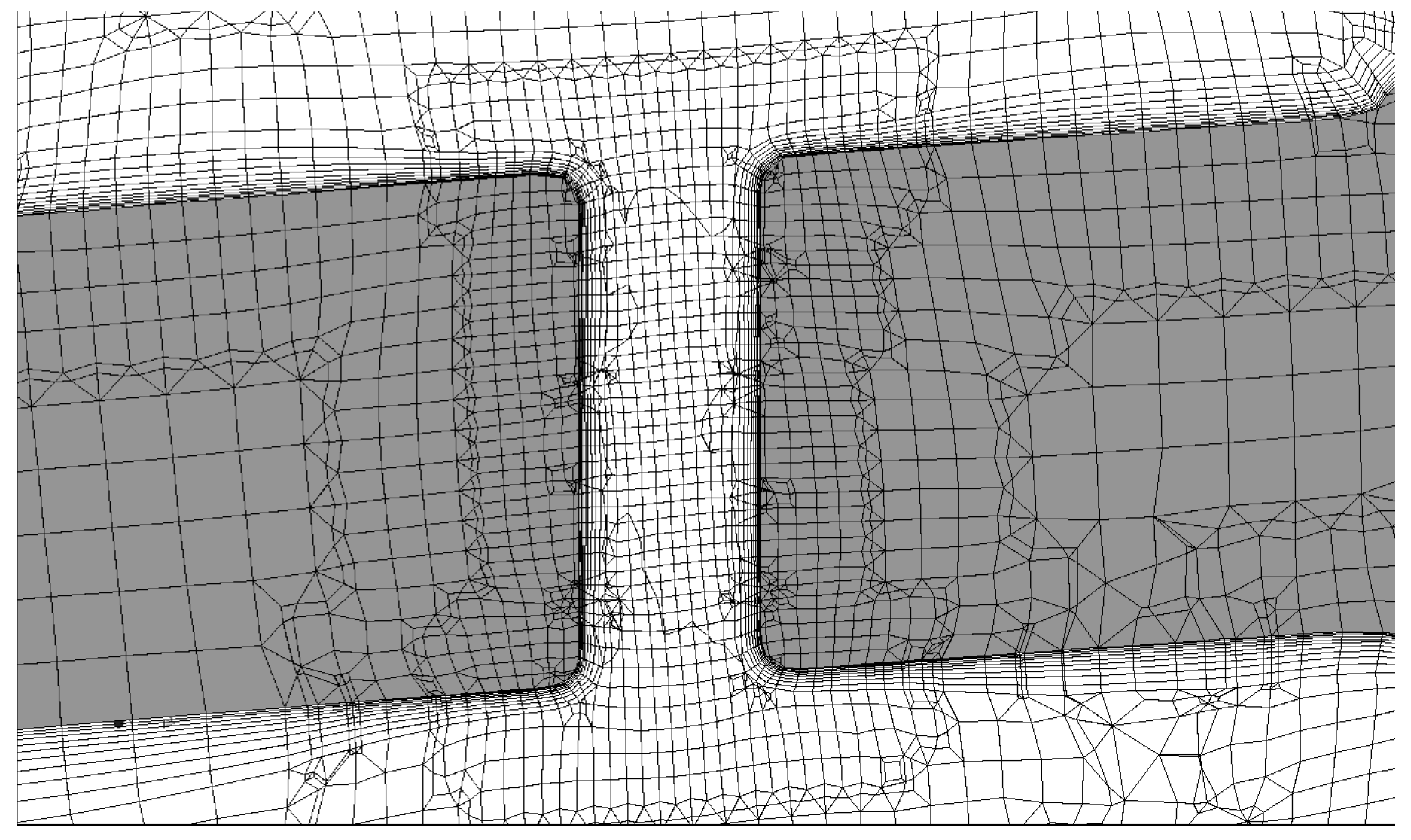
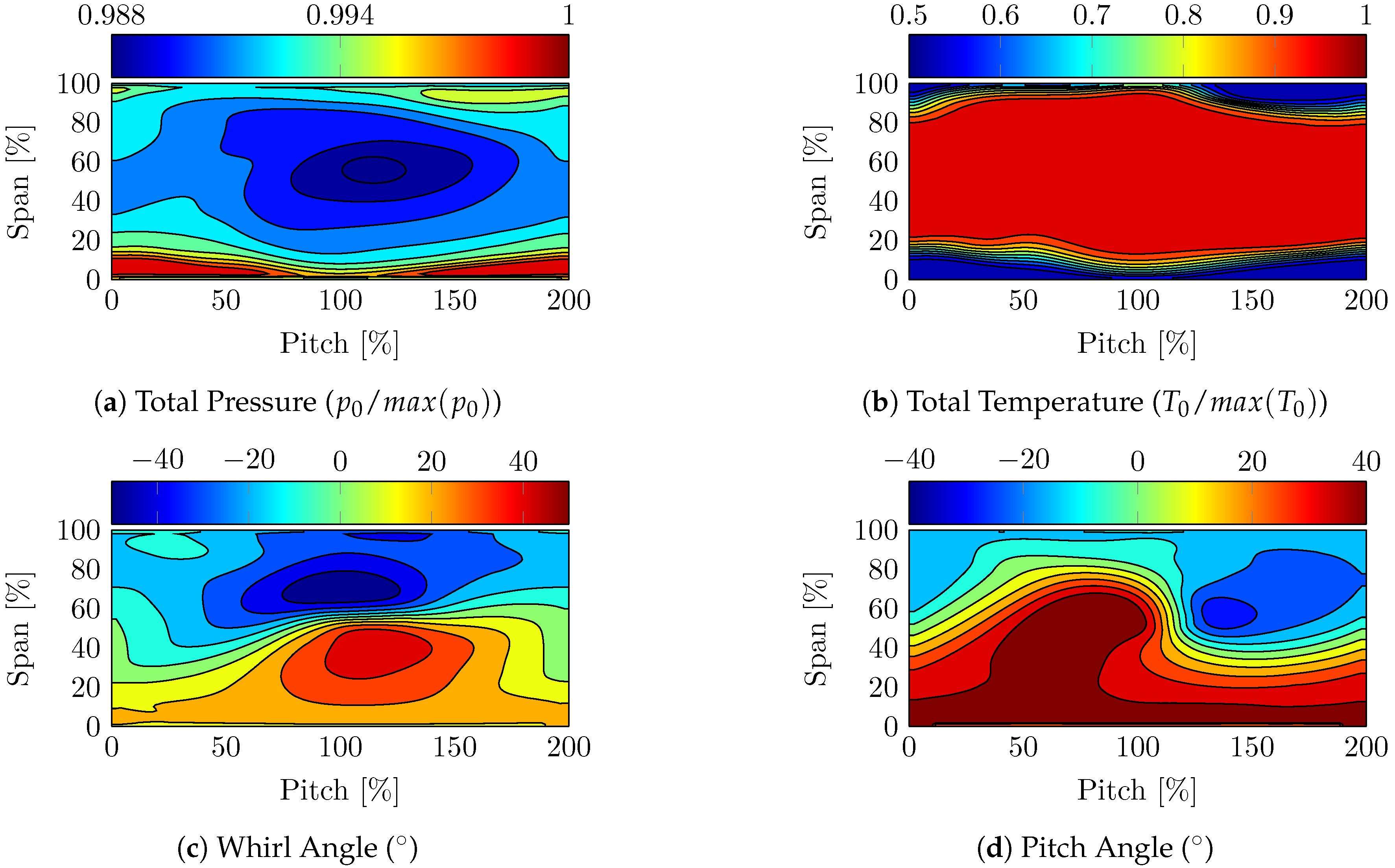
3.1.2. Thermal-Fluid Analysis (CFD)
3.1.3. Structural Analysis (FEA)
3.2. Objectives
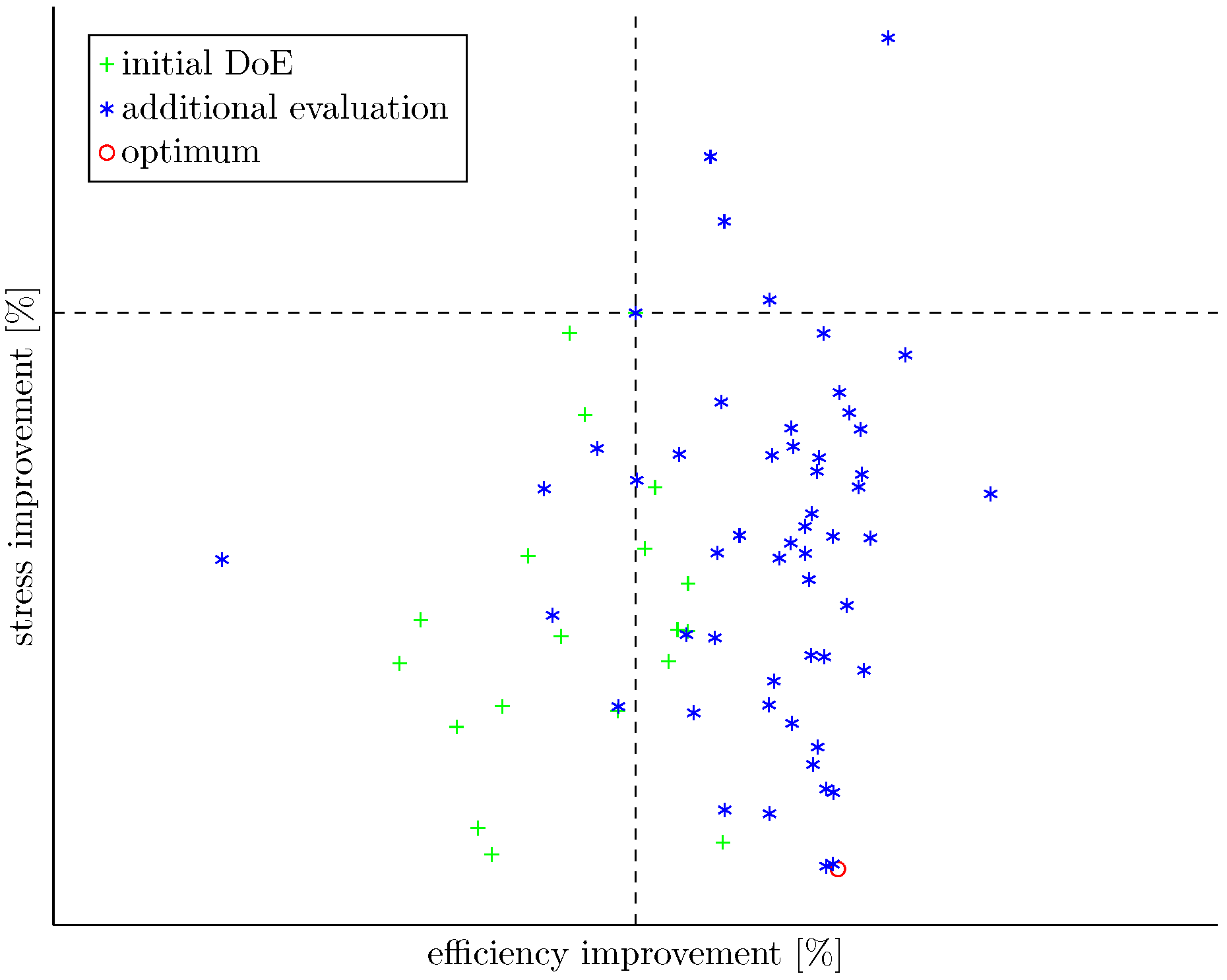
3.3. Optimisation History
4. Study of the Optimum
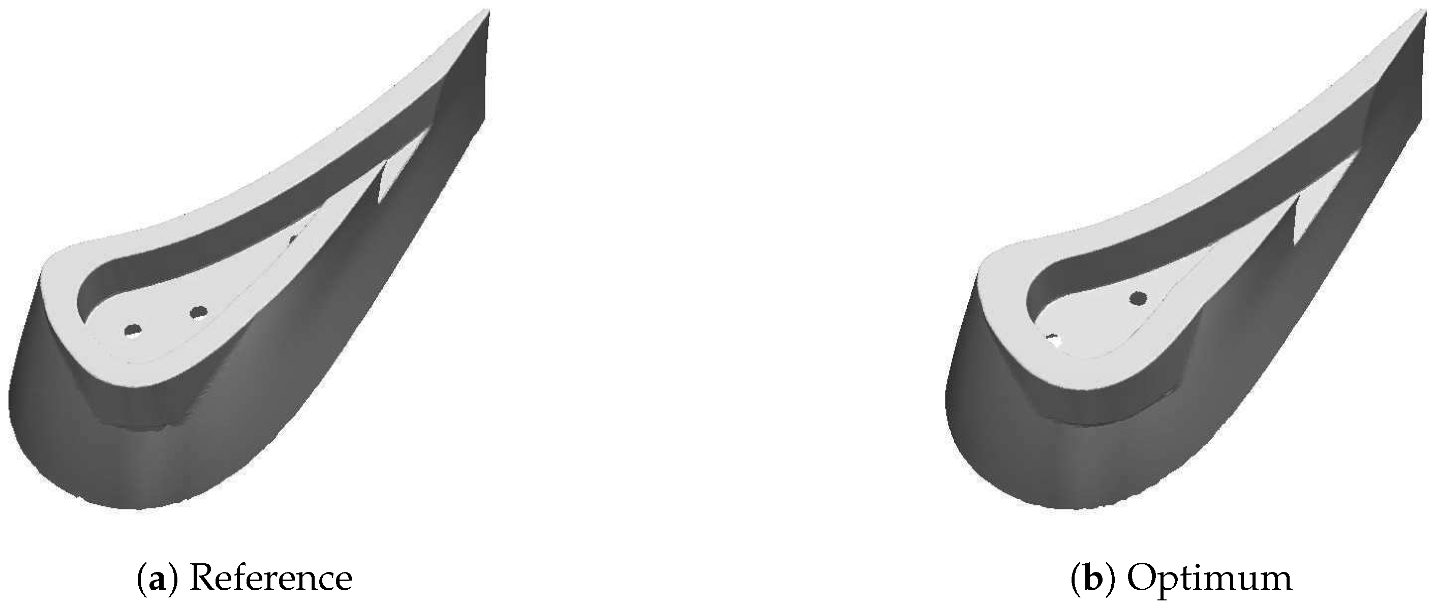
4.1. Geometry
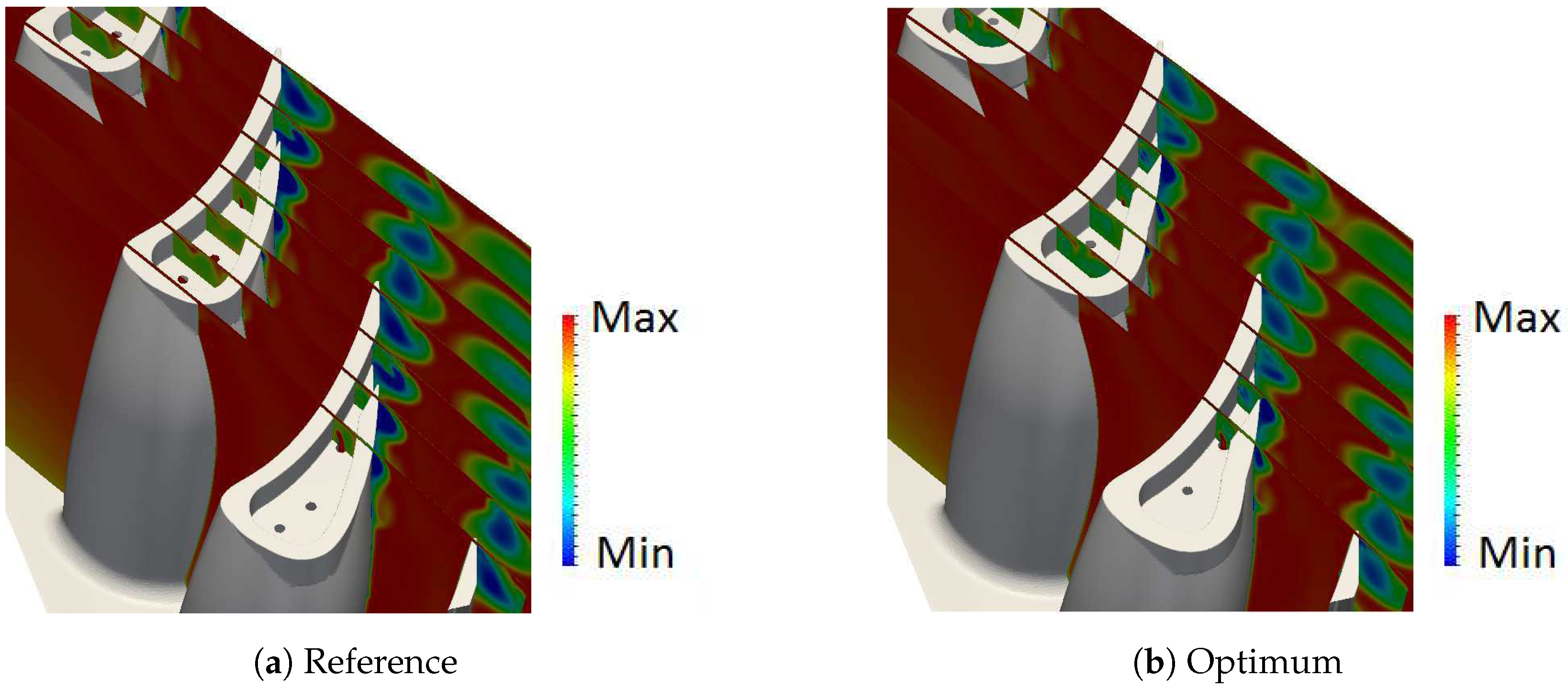
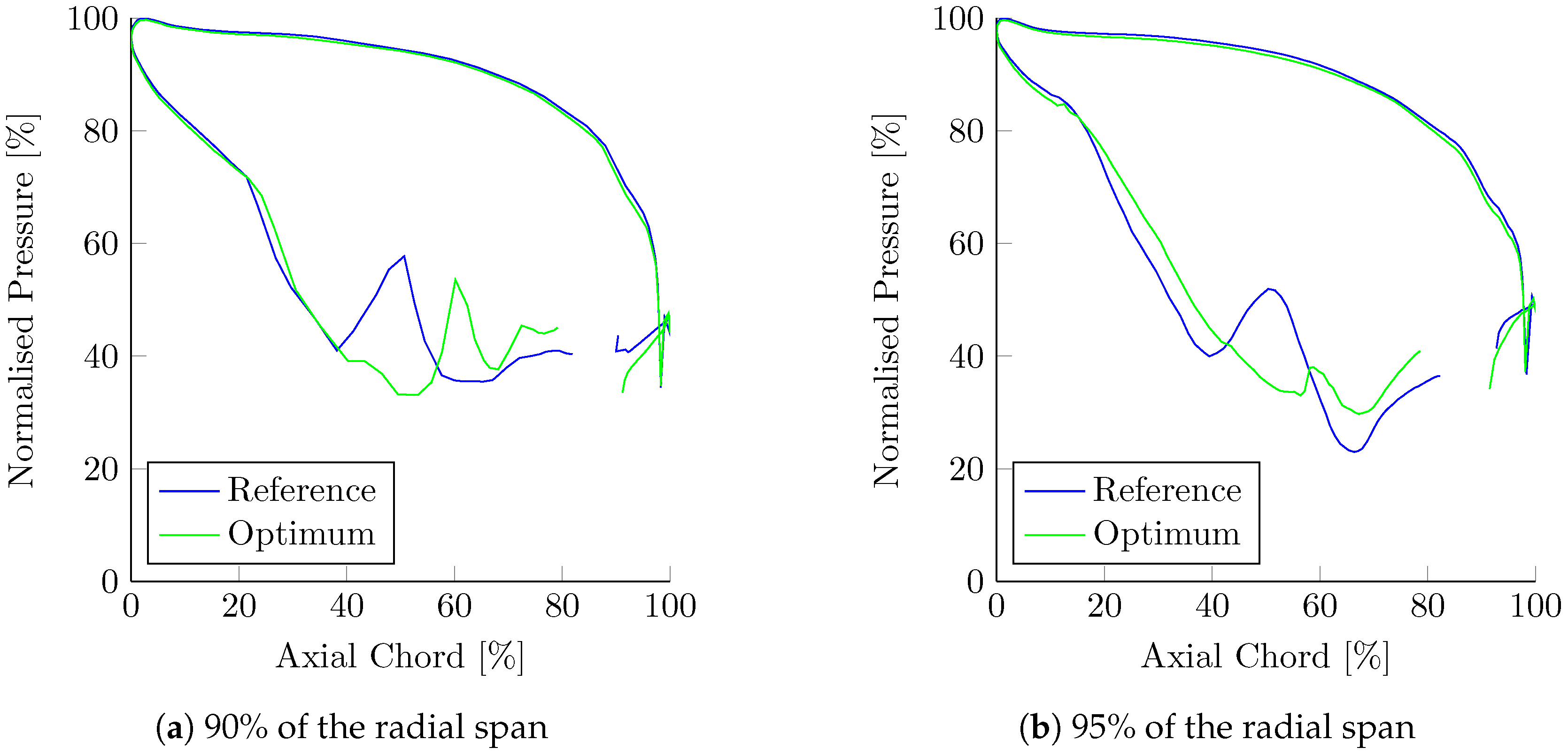
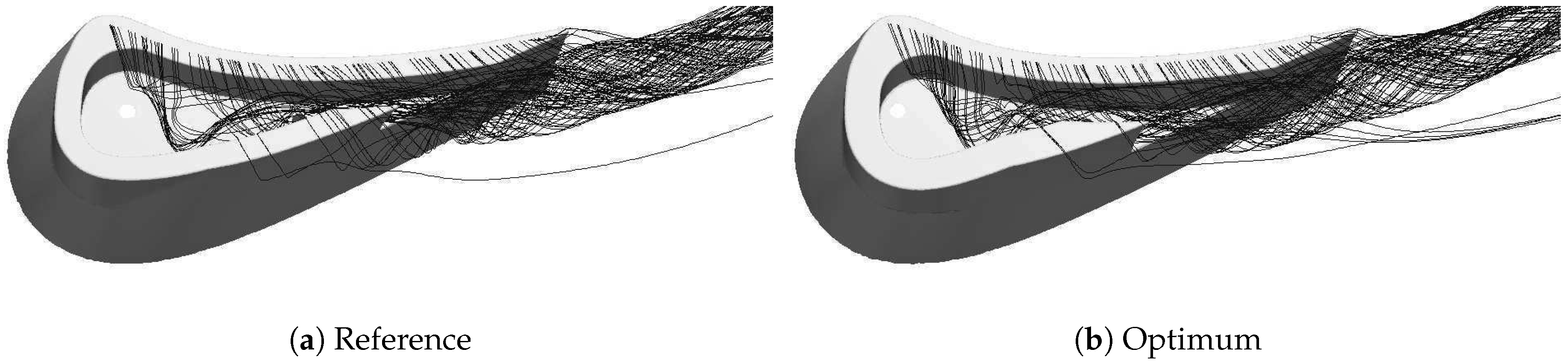
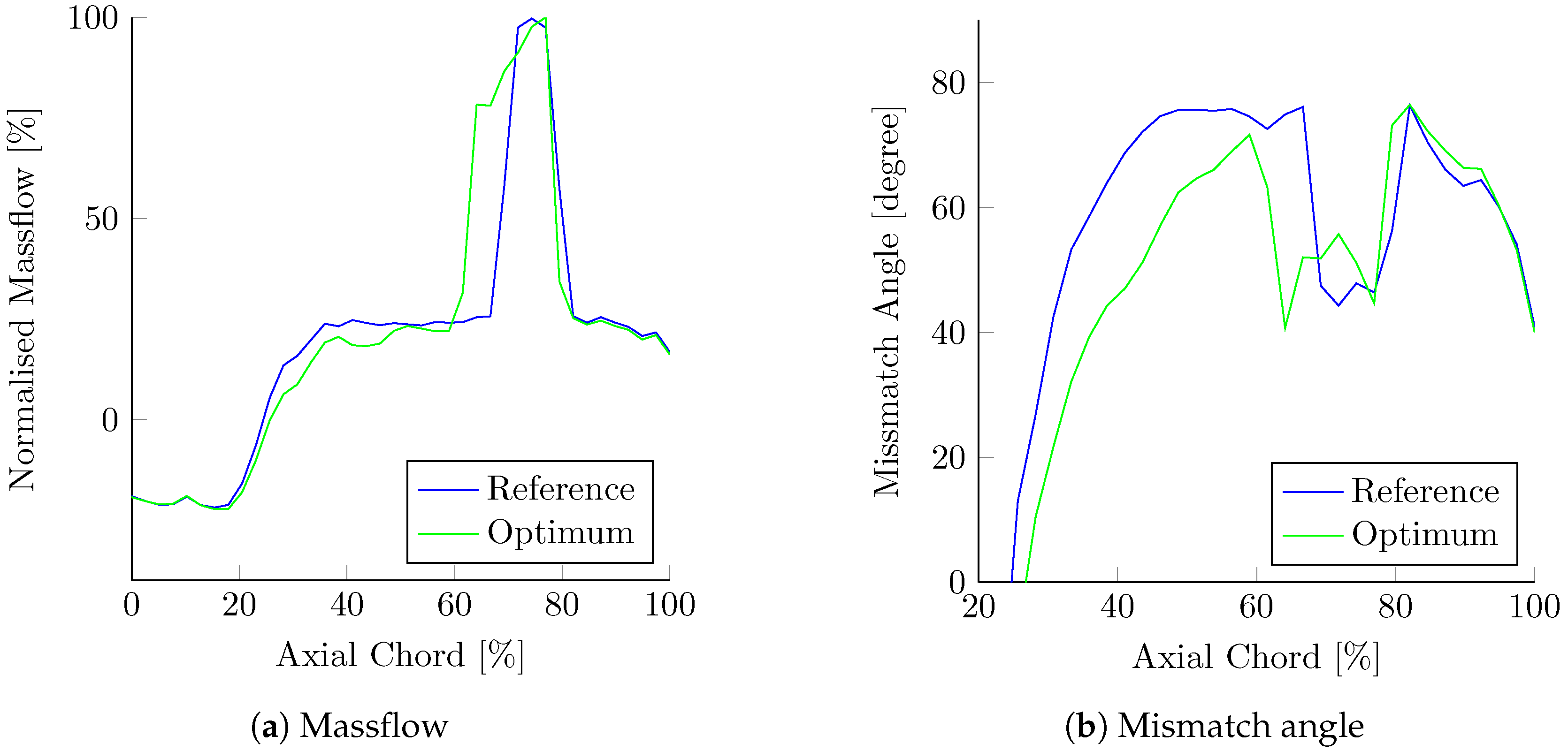
4.2. Aerodynamic Consideration
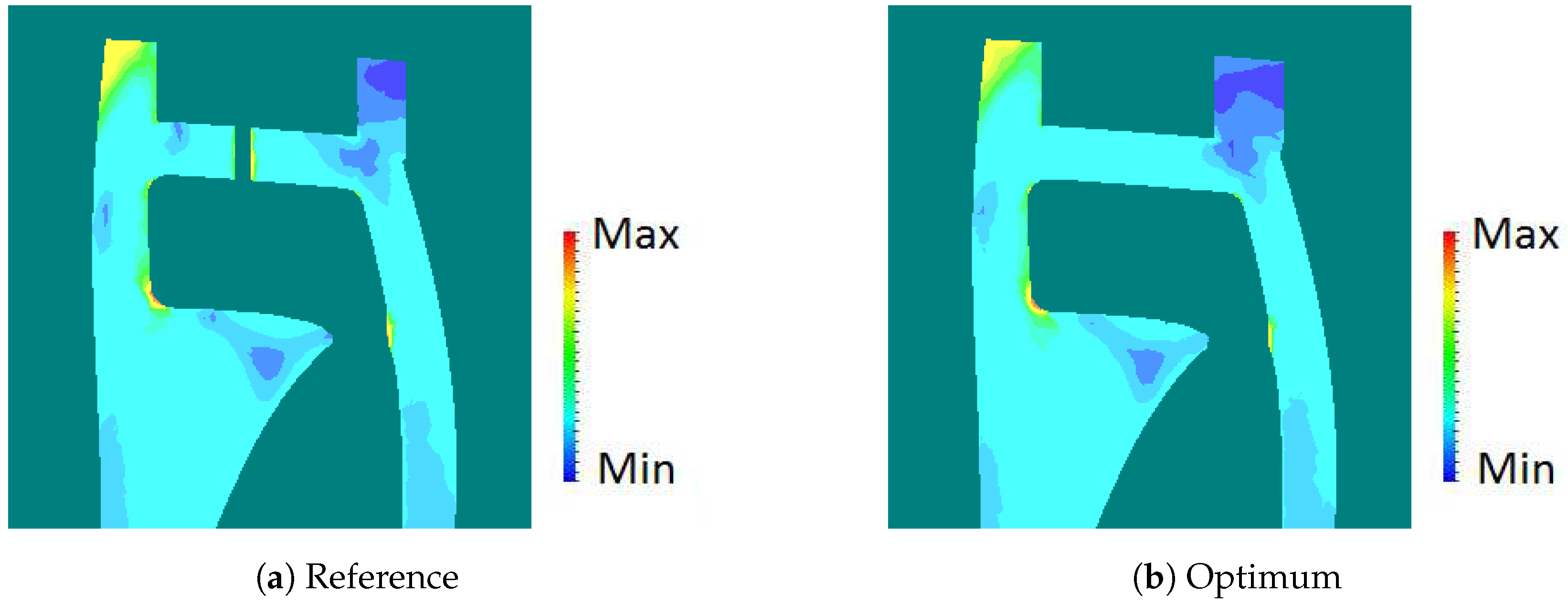
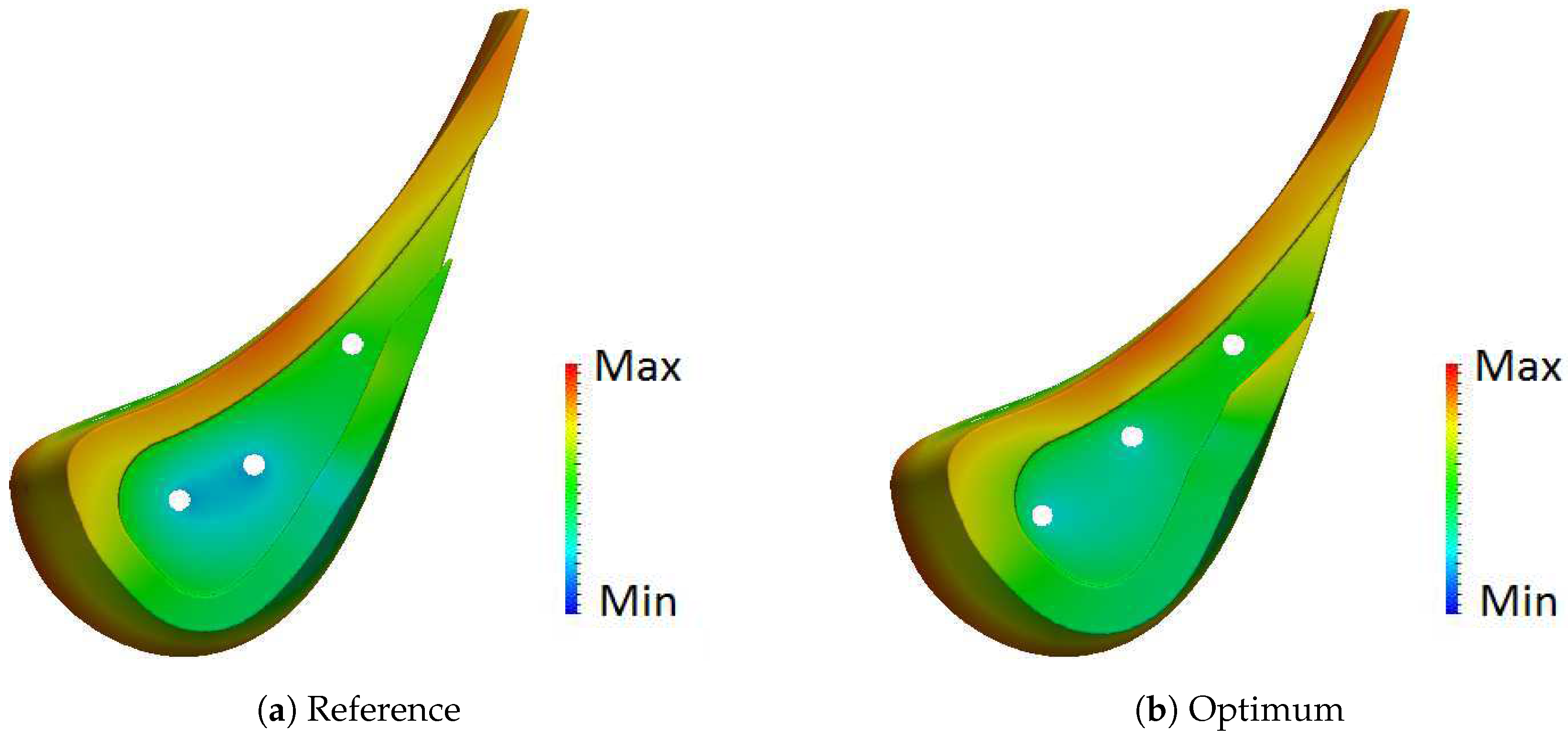
4.3. Thermal and Stress Consideration
5. Conclusions
Author Contributions
Funding
Acknowledgments
Conflicts of Interest
Abbreviations
| Cooling hole horizontal angle | |
| Cooling hole vertical angle | |
| Equivalent adiabatic efficiency | |
| Stress component | |
| Bound value | |
| Whirl angle | |
| c | Constraint value |
| d | Depth |
| Dust dole | |
| Objective function | |
| Constraint function | |
| Design vector | |
| n | Number of objectives |
| N | Number of design variables |
| m | Number of constraints |
| p | Pressure |
| t | Thickness |
| T | Temperature |
| Q | Design space |
| w | Width |
| ARMOGA | Adaptive Range Multi-Objective Genetic Algorithm |
| CAD | Computer aided design |
| CFD | Computational fluid dynamic |
| CHT | Conjugate heat transfer |
| DoE | Design of experiment |
| FE | Finite element |
| HD | Heavy duty |
| LE | Leading edge |
| MAM | Multipoint approximation method |
| MDO | Multi-disciplinary design optimisation |
| OTL | Over tip leakage |
| PS | Pressure side |
| RANS | Reynolds-averaged Navier-Stokes equations |
| SS | Suction side |
| SST | Shear stress transport |
| TE | Trailing edge |
References
- Harvey, N.W. Aerothermal Implications of Shroudless and Shrouded Blades; VKI Lecture Series 2004; Von Karman Institute for Fluid Dynamics: Sint-Genesius-Rode, Belgium, 2004. [Google Scholar]
- Harvey, N.W.; Ramsden, K. A computational study of a novel turbine rotor partial shroud. J. Turbomach. 2001, 123, 534–543. [Google Scholar] [CrossRef]
- Yoon, S.; Curtis, E.; Denton, J.D.; Longley, J.P. The effect of clearance on shrouded and unshrouded turbines at two levels of reaction. J. Turbomach. 2014, 136, 021013. [Google Scholar] [CrossRef]
- Bunker, R.S. Blade Tip Heat Transfer and Cooling Techniques; VKI lecture series 2004; Von Karman Institute for Fluid Dynamics: Sint-Genesius-Rode, Belgium, 2004. [Google Scholar]
- Ameri, A.A.; Steinthorsson, E.; Rigby, D.L. Effect of squealer tip on rotor heat transfer and efficiency. J. Turbomach. 1998, 120, 753–759. [Google Scholar] [CrossRef]
- Coull, J.D.; Atkins, N.R.; Hodson, H.P. Winglets for improved aerothermal performance of high pressure turbines. J. Turbomach. 2014, 136, 091007. [Google Scholar] [CrossRef]
- Coull, J.D.; Atkins, N.R.; Hodson, H.P. High efficiency cavity winglets for high pressure turbines. In Proceedings of the ASME Turbo Expo 2014: Turbine Technical Conference and Exposition, Düsseldorf, Germany, 16–20 June 2014. [Google Scholar]
- Schabowski, Z.; Hodson, H.P.; Giacche, D.; Power, B.; Stokes, M.R. Aeromechanical optimisation of a winglet-squealer tip for an axial turbine. J. Turbomach. 2014, 136, 071004. [Google Scholar] [CrossRef]
- Lomakin, N.; Granovskiy, A.; Shchaulov, V.; Szwedowicz, J. Effect of Various Tip Clearance Squealer Design on Turbine Stage Efficiency. In Proceedings of the ASME Turbo Expo 2015: Turbine Technical Conference and Exposition, Montreal, QU, Canada, 15–19 June 2015. [Google Scholar]
- Caloni, S.; Shahpar, S. Multi-Disciplinary Analyses for the Design of a High Pressure Turbine Blade Tip. In Proceedings of the ASME Turbo Expo 2016: Turbine Technical Conference and Exposition, Seoul, Korea, 13–17 June 2016. [Google Scholar]
- Caloni, S.; Shahpar, S.; Coull, J.D. Numerical Investigations of Different Tip Designs for Shroudless Turbine Blades. In Proceedings of the 11th European Turbomachinery Conference, At Madrid, Spain, 23–27 March 2015; pp. 1–13. [Google Scholar]
- Martins, J.R.R.A.; Lambe, A.B. Multidisciplinary design optimization: a survey of architectures. AIAA J. 2013, 51, 2049–2075. [Google Scholar] [CrossRef]
- Toropov, V.V. Simulation approach to structural optimization. Struct. Optim. 1989, 1, 37–46. [Google Scholar] [CrossRef]
- Toropov, V.V.; Filatov, A.A.; Polynkin, A. Multiparameter structural optimization using FEM and multipoint explicit approximations. Struct. Optim. 1993, 6, 7–14. [Google Scholar] [CrossRef]
- Polynkin, A.; Toropov, V.V. Mid-range metamodel assembly building based on linear regression for large scale optimization problems. Struct. Multidiscip. Optim. 2012, 45, 515–527. [Google Scholar] [CrossRef]
- Lancaster, P.; Salkauskas, K. Surfaces generated by moving least squares methods. Math. Comput. 1981, 37, 141–158. [Google Scholar] [CrossRef]
- Van Keulen, F.; Toropov, V.V. New developments in structural optimization using adaptive mesh refinement and multipoint approximations. Eng. Optim. 1997, 29, 217–234. [Google Scholar] [CrossRef]
- Olhoff, N. Multicriterion structural optimization via bound formulation and mathematical programming. Struct. Optim. 1989, 1, 11–17. [Google Scholar] [CrossRef]
- Caloni, S.; Shahpar, S. Investigation Into Coupling Techniques for a High Pressure Turbine Blade Tip. In Proceedings of the 11th European Turbomachinery Conference, At Madrid, Spain, 23–27 March 2015. [Google Scholar]
- Coull, J.D.; Atkins, N.R. The influence of boundary conditions on tip leakage flow. J. Turbomach. 2015, 137, 061005. [Google Scholar] [CrossRef]
- Khanal, L.; He, L.; Northall, J.; Adami, P. Analysis of Radial Migration of Hot-Streak in Swirling Flow Through HP Turbine Stage. J. Turbomach. 2013, 135, 041005. [Google Scholar] [CrossRef]
- Demargue, A.A.; Evans, R.O.; Tiller, P.J.; Dawes, W.N. Practical and reliable mesh generations for complex real-world geometries. In Proceedings of the 52nd Aerospace Sciences Meeting, National Harbor, MD, USA, 13–17 January 2014. [Google Scholar]
- Dawes, W.N.; Kellar, W.P.; Harvey, S.A. Using level sets as the basis for a scalable, parallel geometry engine and mesh generation system. In Proceedings of the 47th AIAA Aerospace Sciences Meeting including The New Horizons Forum and Aerospace Exposition, Orlando, FL, USA, 5–8 January 2009. [Google Scholar]
- Moinier, P.; Giles, M.B. Preconditioned Euler and Navier-Stokes Calculations on Unstructured Grids. In Proceedings of the 6th ICFD Conference on Numerical Methods for Fluid Dynamics, Oxford, UK, 31 March–3 April 1998. [Google Scholar]
- Atkins, N.R.; Ainsworth, R.W. Turbine aerodynamic performance measurements under nonadiabatic conditions. J. Turbomach. 2012, 134, 061001. [Google Scholar] [CrossRef]
- Verstraete, T. Multidisciplinary Turbomachinery Component Optimisation Considering Performance, Stress and Internal Heat Transfer. Ph.D. Thesis, Universiteit Gent, Gent, Belgium, June 2008. [Google Scholar]
- Kazimi, S.M.A. Solid Mechanics; McGraw-Hill Education: NewYork, NY, USA, 1982. [Google Scholar]
- Dawes, W.N.; Kellar, W.P.; Richardson, G.A. Application of topology-free optimization to manage cooled turbine tip heat load. In Proceedings of the ASME Turbo Expo 2009: Power for Land, Sea, and Air, Orlando, FL, USA, 8–12 June 2009. [Google Scholar]
- Denton, J.D. Loss mechanisms in turbomachines. J. Turbomach. 1993, 115, V002T14A001. [Google Scholar] [CrossRef]


| Leakage | Reference | Optimum |
|---|---|---|
| Total | ||
| Over SS rim | ||
| Through TE opening | ||
| Ratio |
© 2018 by the authors. Licensee MDPI, Basel, Switzerland. This article is an open access article distributed under the terms and conditions of the Creative Commons Attribution (CC BY) license (http://creativecommons.org/licenses/by/4.0/).
Share and Cite
Caloni, S.; Shahpar, S.; Toropov, V.V. Multi-Disciplinary Design Optimisation of the Cooled Squealer Tip for High Pressure Turbines. Aerospace 2018, 5, 116. https://doi.org/10.3390/aerospace5040116
Caloni S, Shahpar S, Toropov VV. Multi-Disciplinary Design Optimisation of the Cooled Squealer Tip for High Pressure Turbines. Aerospace. 2018; 5(4):116. https://doi.org/10.3390/aerospace5040116
Chicago/Turabian StyleCaloni, Stefano, Shahrokh Shahpar, and Vassili V. Toropov. 2018. "Multi-Disciplinary Design Optimisation of the Cooled Squealer Tip for High Pressure Turbines" Aerospace 5, no. 4: 116. https://doi.org/10.3390/aerospace5040116
APA StyleCaloni, S., Shahpar, S., & Toropov, V. V. (2018). Multi-Disciplinary Design Optimisation of the Cooled Squealer Tip for High Pressure Turbines. Aerospace, 5(4), 116. https://doi.org/10.3390/aerospace5040116