Active Control of Laminar Separation: Simulations, Wind Tunnel, and Free-Flight Experiments

Abstract

When a laminar boundary layer is subjected to an adverse pressure gradient, laminar separation bubbles can occur. At low Reynolds numbers, the bubble size can be substantial, and the aerodynamic performance can be reduced considerably. At higher Reynolds numbers, the bubble bursting can determine the stall characteristics. For either setting, an active control that suppresses or delays laminar separation is desirable. A combined numerical and experimental approach was taken for investigating active flow control and its interplay with separation and transition for laminar separation bubbles for chord-based Reynolds numbers of Re ≈ 64,200–320,000. Experiments were carried out both in the wind tunnel and in free flight using an instrumented 1:5 scale model of the Aeromot 200S, which has a modified NACA 64₃-618 airfoil. The same airfoil was also used in the simulations and wind tunnel experiments. For a wide angle of attack range below stall, the flow separates laminar from the suction surface. Separation control via a dielectric barrier discharge plasma actuator and unsteady blowing through holes were investigated. For a properly chosen actuation amplitude and frequency, the Kelvin–Helmholtz instability results in strong disturbance amplification and a “roll-up” of the separated shear layer. As a result, an efficient and effective laminar separation control is realized.

1. Introduction

Laminar separation bubbles (LSBs) form when a laminar boundary layer detaches from a surface, undergoes transition, and reattaches as a transitional or turbulent flow. At low Reynolds number conditions (up to Re ≈ 300,000), LSBs can significantly affect the aerodynamic performance of lifting surfaces even at low angles of attack (AoAs). For example, for small fixed and rotary wing unmanned aerial vehicles (UAVs), the flow can separate at the beginning of the adverse pressure gradient, and the LSB can extend over a significant portion of the airfoil. At larger Reynolds numbers (Re ≈ 1 million), LSBs play an important role for laminar flow airfoils. For such airfoils at the design AoA, short and shallow LSBs trip the boundary layers to turbulence. As the AoA is increased (such as during a pitch-up maneuver), the suction-side LSB migrates to the leading edge, and the turbulent trailing edge separation begins to slowly “creep” upstream. At some critical AoA, the LSB will suddenly open up or “burst”, and the flow will separate laminar from the leading edge. The resulting abrupt drop in lift is known as “hard stall”, and has to be avoided during routine operation. This sequence of events has recently been revealed in great detail in large-eddy simulations by Benton and Visbal [1,2]. The bursting of LSBs was first investigated by Gaster [3], who also proposed a bursting criterion. The understanding of the flow physics of LSBs, which are governed by laminar separation, transition, and turbulent reattachment, as well as “external influences” such as wall roughness and free-stream turbulence, appear to be of critical importance for the prediction and control of the LSB formation and bubble bursting. The LSB physics are typically investigated at low Reynolds number conditions (Re ≈ 100,000) where the relative size of the bubble with respect to a relevant body dimension (such as the airfoil chord) is large. This approach is motivated by the greater ease of instrumentation (in the experiment) and the lower computational expense (of simulations) compared to similar investigations at high Reynolds number conditions (Re ≈ 1 million and beyond).

The amount of literature concerned with laminar separation and its control is immense, and in the following, only a few papers shall be cited that are more directly related to the research in this paper. Hain et al. [4] carried out time-resolved particle image velocimetry (PIV) measurements in the water tunnel for a wing section with an SD 7003 airfoil at a chord Reynolds number of 66,000. At α = 4 degrees angle of attack (AoA), an LSB was observed. It was found that Kelvin–Helmholtz instabilities resulted in the generation and amplification of spanwise “rollers” in the shear layer above the bubble, which then lead to three-dimensional (3D) breakdown to turbulence. Jones et al. [5] employed direct numerical simulations (DNS) for investigating LSBs on an NACA 0012 airfoil at Re ≈ 50,000 and α = 5 degrees. Volume forcing upstream of the bubble was shown to promote transition to turbulence and increase the aerodynamic performance. When the forcing was discontinued, the turbulence was self-sustained. Based on a series of simplified 3D simulations, it was concluded that the naturally occurring two-dimensional (2D) vortex shedding makes the flow absolutely unstable to 3D perturbations.

Seifert et al. [6] demonstrated the great potential of active flow control (AFC) for delaying stall on an airfoil. Periodic actuation at a reduced frequency that was slightly higher than the natural vortex shedding frequency required 90% less momentum than a steady actuation for obtaining a similar performance gain. Pulsed vortex generator jets (VGJs) have been investigated extensively, both experimentally and numerically, for suppressing LSBs on low-pressure turbine (LPT) blades (e.g., Bons et al. [7], Postl et al. [8]). The stunning performance of pulsed VGJs was attributed to the in-phase actuation of the jets, which introduces 2D disturbances that are amplified by the flow (at no cost), as the result of a hydrodynamic instability (e.g., Postl et al. [8], Gross et al. [9]). Wind-tunnel experiments for an LPT blade with a steady and pulsed dielectric barrier discharge (DBD) actuator were carried out by Huang et al. [10,11]. For steady actuation, the flow was tripped to turbulence. The optimum reduced frequency for pulsed actuation was found to be unity. The generation of spanwise flow structures that promote mixing was identified as the dominant mechanism. Gaitonde et al. [12] developed and validated a DBD actuator model for use in simulations. The high effectiveness of DBD actuators for controlling laminar separation from LPT blades was also demonstrated in simulations by e.g., Rizzetta and Visbal [13]. Visbal et al. [14] carried out simulations for investigating separation control by a DBD actuator for a wing section. Pulsed actuation was found to be more effective than steady actuation. It was concluded that transition and turbulence enhancement mechanisms are of greater importance for an effective control than the steady wall–jet momentum injection. Benton and Visbal [1,2] investigated the bubble bursting for a wing section during a pitch-up maneuver for chord-based Reynolds numbers between 200,000 and 1,000,000. When 2D disturbances were introduced upstream of separation, the bubble bursting could be significantly delayed. The control was more effective when the forcing frequency was larger than the most amplified frequency predicted by linear stability theory (LST).

Active flow control of laminar separation can also be employed for the hingeless maneuvering of small aircraft that are operated at low chord Reynolds numbers. Already in 2002, Fasel et al. at the University of Arizona demonstrated a successful roll control for a model aircraft (Cain et al. [15]). Wing tip extensions were added to the original model. The extensions were shaped to harbor a relatively large LSB on the suction surface near the trailing edge. Using AFC by pulsed VGJs, separation was suppressed on either one of the wing tip extensions, which resulted in a roll moment. Later wind tunnel and model flight experiments by Ciuryla et al. [16] and Seifert et al. [17] also demonstrated a successful roll control with AFC-equipped wing sections. The focus of this earlier flight research was more on the successful active control of separation, and less on the detailed understanding of the flow physics of LSBs.

Laminar boundary layers have a lower skin friction drag than turbulent boundary layers. However, they are also more prone to separate in the presence of adverse pressure gradients. Airfoils with significant laminar run may display poor performance when operated at below design Reynolds numbers. Thus, they lend themselves to investigations aimed at understanding the flow physics of laminar separation and transition and its active control. Since tunnel noise has an effect on transition, and because the free-stream turbulence intensity in the atmosphere is typically very low in the early morning hours, flight experiments seem to be a natural choice for such investigations. Wing gloves that slide over the wing of an existing aircraft without compromising its structure or adversely affecting its aerodynamics have a long history in laminar flow control research. Laminar flow control refers to the delay of laminar turbulent transition. Although this subject is only indirectly related to laminar flow control, in the following, a brief survey of earlier laminar flow control experiments with wing gloves is provided with a focus on the instrumentation as relevant for laminar separation control (LSC) flight research. Already in 1941, the National Aeronautics and Space Administration (NASA) flew a wing glove on a B18, and later in the 1950s, a laminar flow wing glove was flown on a de Havilland Vampire. Many more laminar flow wing glove experiments followed (Braslow [18]). Recently, researchers at the Technical University of Darmstadt flew a wing glove on a Grob G109b motor glider. The advantage of using a motor glider is that measurements can be performed while soaring, i.e., with the engine turned off, to reduce disturbances due to engine noise or engine-induced vibrations. The wing glove was instrumented with multi-sensor hot films, piezofoil arrays, and a miniaturized laser Doppler velocimetry probe. A ceramic insert that was connected to a loudspeaker served as a disturbance source (Nitsche et al. [19]). In later flight experiments, a DBD plasma actuator was employed for introducing disturbances, and microphone and hot-wire measurements were taken (Duchmann et al. [20]). Researchers at the Technical University of Berlin flew a wing glove on a Grob G103 TWIN II sailplane (Peltzer et al. [21,22]). The wing glove was equipped with a membrane actuator and surface hot-wire sensors. Researchers at Texas A&M developed a wing glove for a Gulfstream III for investigating discrete roughness elements for delaying transition (Belisle et al. [23]).

This article provides a comprehensive summary of a multi-year research program that was executed at the University of Arizona with funding from the Air Force Office of Scientific Research. The focus of the project was on understanding the flow physics of LSBs and the interaction of separation, transition, and AFC. The paper brings together results from several earlier conference and journal papers, as well as formerly unpublished research, and makes a connection between simulations, wind tunnel, and free-flight experiments. The outcome is a synergistic strategy for transferring active flow control technologies from the laboratory to actual flight hardware.

2. Investigative Methods

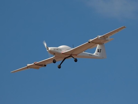
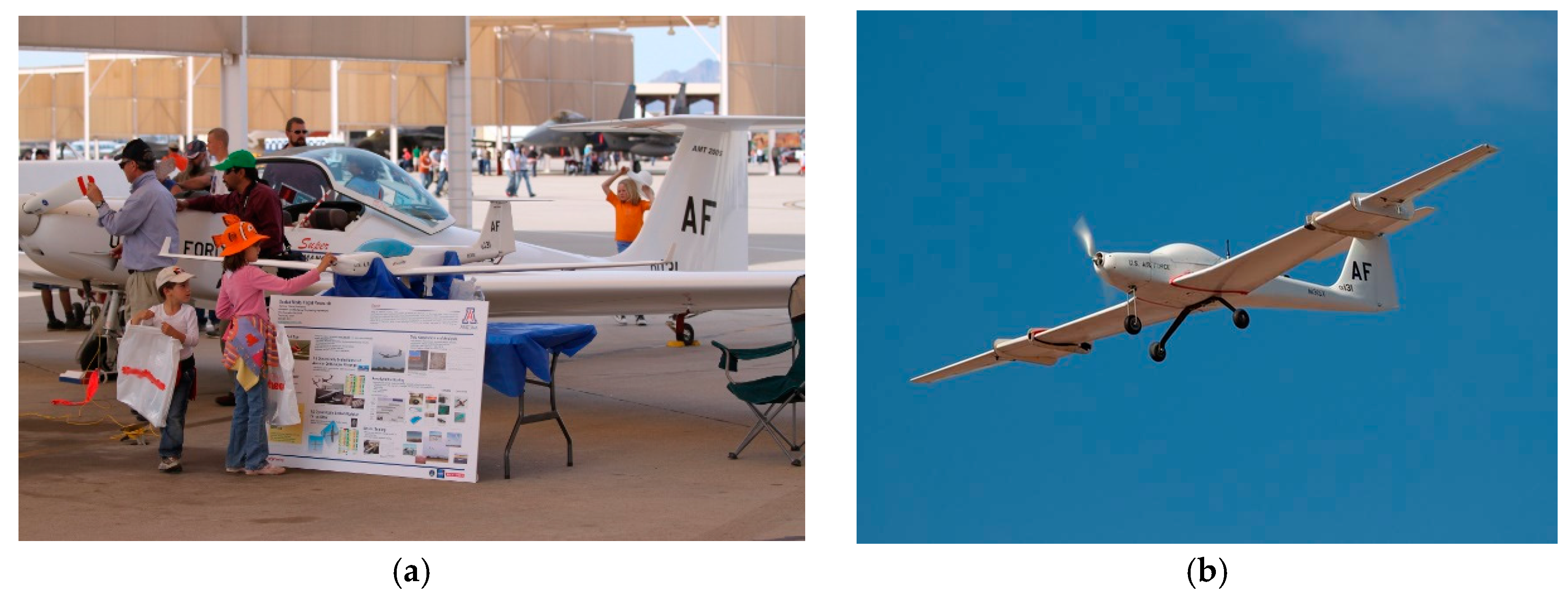
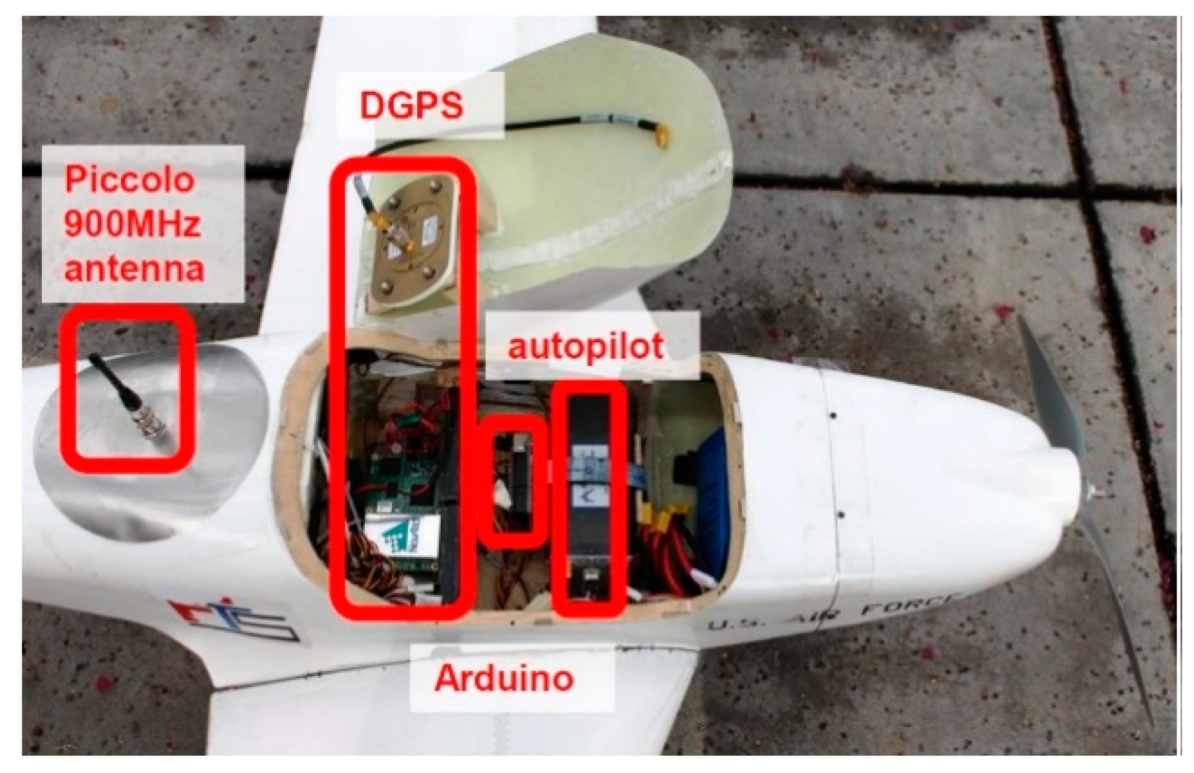
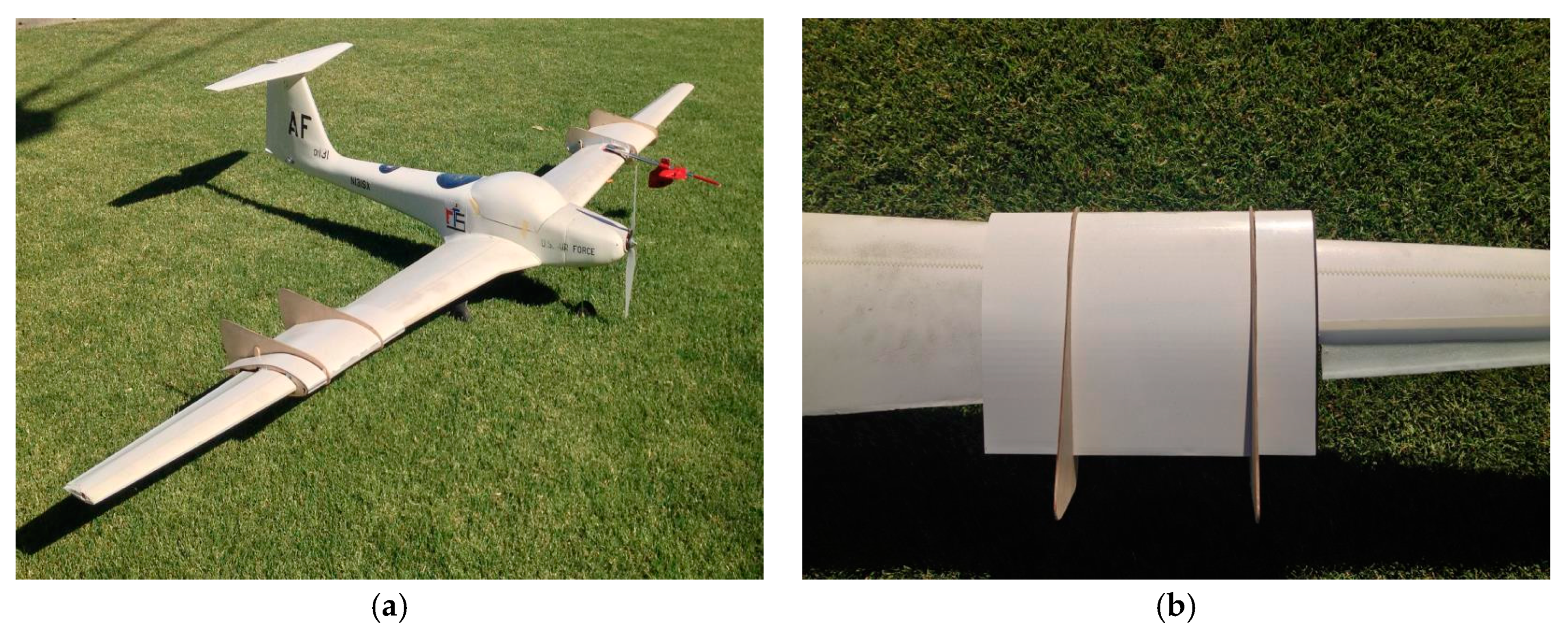
2.1. Flight Experiments

The research project was motivated by the idea to develop AFC technologies in the lab (simulations and wind tunnel experiments) and to transition them to a full-size aircraft via scaled model flight experiments. Early on, it was decided to use the airfoil of a full-size aircraft for the wind tunnel experiments and simulations. The class of aircraft was narrowed down to motor gliders, which were determined to be ideal for laminar flow control free-flight experiments. They can motor to altitude; the motor is then turned off for obtaining a low-disturbance flight test environment (e.g., Duchmann et al. [20]). As a result of their low induced drag high-aspect ratio wings, the motor-off glide times are relatively long. The Aeromot (AMT) 200S Super Ximango motor glider was chosen, because a full-size plane of this type was available for private use. Within the framework of a NASA Small Business Technology Transfer (STTR) program, two 1:5 scale AMT 200S were developed and built from the ground up for low-cost flight experiments [24] (Figure 1). The models were dynamically scaled according to the dynamic scaling laws (e.g., Wolowicz et al. [25], Gainer and Hoffman [26]). For an example of the development of a dynamically scaled Boeing 757 model, see Jordan et al. [27]. Dynamic scaling requires Froude number similarity. If aerodynamic similarity was obtained as well, the full-size aircraft’s stability, control, and handling qualities would be accurately replicated by the scaled aircraft. The modified NACA 64₃-618 airfoil of the AMT 200S was also chosen for the wind tunnel experiments and simulations. During the scaled model free-flight experiments, wind tunnel experiments, and simulations, the airfoil was operated below its design Reynolds number, and large LSBs formed at the beginning of the adverse pressure gradient region on the top and bottom surface at low AoAs (e.g., during cruise). As the AoA was increased and the Reynolds number was lowered (e.g., as stall is approached), the LSB on the suction surface grew to appreciable size. Since the focus of the research program was on laminar separation and its control, this effect was desired.

The AMT 200S has a wingspan of 17.5 m, an empty mass of 604 kg, and a maximum gross mass of 850 kg (Figure 1a). The 1:5 scale model has a wingspan of 3.5 m, an empty mass of 4.8 kg, and a maximum takeoff mass of 9.5 kg (Figure 1b). The model is powered by an electric motor and allows for flight test times in excess of 15 min. The measured stall speed is 11.3 m/s, and the takeoff speed is 12.9 m/s. The model can be flown manually (via remote control) or autonomously (via a Cloud Cap Piccolo 2 autopilot). A Novatel differential GPS with 3-cm accuracy is available for accurate positioning and ground speed measurements (Figure 2). The autopilot allows the model to maintain straight and level flight for accurate flight experiments at constant free-stream conditions. The altitude and air speed can be held with an accuracy of ±0.6 m and ±1 m/s, respectively. Characteristic Reynolds numbers based on wing tip chord and mean aerodynamic chord (MAC) are provided in

Table 1. Chord-based Reynolds numbers. MAC: mean aerodynamic chord.

Aircraft and Airspeed	Reference Length	Reynolds Number
1:5 scale takeoff	Wing tip chord	64,200
1:5 scale takeoff	MAC	137,000
1:5 scale cruise	MAC	320,000
Full-size slow flight (26.8 m/s)	MAC	1,500,000
Full-size cruise (56.6 m/s)	MAC	3,200,000

.

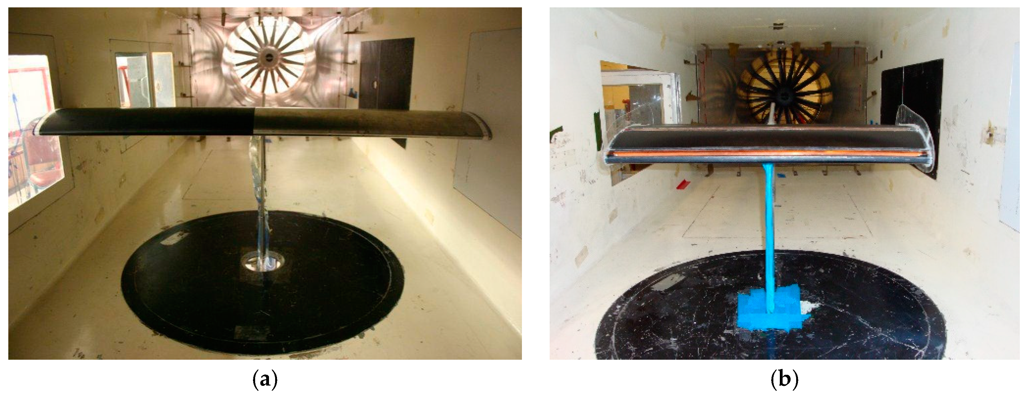
2.2. Wind Tunnel Experiments

Detailed wind tunnel experiments were carried out for the NACA 64₃-618 airfoil of the AMT 200S. This laminar flow airfoil has a maximum relative thickness of 18%. The maximum thickness is located at 40% of the chord, which is also where the adverse pressure gradient starts. All of the wind tunnel experiments (except for the wing glove experiments, which will be discussed later) were carried out in an open return subsonic wind tunnel with a 0.91-m tall and 1.2-m wide test section at the Aerospace and Mechanical Engineering (AME) Department at the University of Arizona. Three constant chord wing sections were manufactured for the wind tunnel experiments. Mack et al. [28] built a fiberglass and an aluminum wing section with a chord length of 0.3 m and a span of 1.2 m (Figure 3a). The aluminum model was equipped with 48 pressure taps that were connected to a pressure transducer via a ScaniValve. The tunnel blockage for the two wings was 5.9% at α = 0 degrees and 11.7% at α = 10 degrees. Both wings extended to the tunnel side walls, which improved the two-dimensionality of the flow. Plogmann et al. [29] manufactured a 0.91-m wide fiberglass wing with an 0.3-m chord (Figure 3b) and a tunnel blockage of 4.5% at α = 0 degrees and 8.8% at α = 10 degrees. Boundary-layer fences were added at the wing tips to make the flow more two-dimensional. This wing was manufactured with a carbon fiber cloth underneath the suction-side skin. The carbon fiber serves as an electric resistor for heating the top surface by a small amount (less than 3 K). A Flir A320 infrared camera with a temperature sensitivity of 0.08 K was employed to measure the temperature distribution on the top surface. Since the heat transfer coefficient is proportional to the skin-friction coefficient, areas with high skin friction (such as the turbulent boundary layer) are cooled more strongly than areas with low skin friction (e.g., “dead air” regions), and thus appear colder in the infrared images.

Both models were mounted on a six-component force balance inside the test section of the wind tunnel. The fiberglass models were painted black to allow for oil flow visualizations and to minimize laser reflections (Figure 3). For the former, oil paint that contained white titanium-oxide pigment was mixed with quickly evaporating lighter fluid and slowly evaporating kerosene. The mixture was applied to the top surface of the wing sections, and the tunnel was run until the lighter fluid and kerosene had evaporated. Particle image velocimetry (PIV) measurements were made with a stereoscopic LaVision system. The system consists of a double-pulsed Nd:YAG laser with a wave length of 520 nm and an output of 120 mJ/pulse, as well as two charge-coupled device (CCD) cameras with a resolution of 1600 × 1200 pixels. The cameras were used in two-dimensional independent mode to obtain a wider field of view in the streamwise direction. The light sheet was oriented normal to the span, and had a thickness of approximately 1–2 mm. Olive oil seeding particles were added to the flow upstream of the contraction section of the wind tunnel to ensure uniform seeding. All of the measurements were made in the wing center plane.

For the AFC experiments, the wing sections were equipped with DBD plasma actuators. The electrodes for the fiberglass model by Mack et al. [28] were made from 0.1-mm thick copper-foil tape. The dielectric was made from Kapton and Teflon tape, and had a total thickness of ≈0.5 mm. For the Plogmann et al. [29] wing, the electrodes were made from 0.0254-mm thick copper tape, and the dielectric was made from three layers of Kapton tape with a thickness of 0.0254 mm. For both designs, the two electrodes were overlapping slightly in the streamwise direction. Compared to the result without a plasma actuator (baseline, plain wing), with a plasma actuator at 40% chord (control off), the lift curve deviates later (at a higher AoA) from the linear lift curve slope (Figure 4). The effect is slightly more pronounced when the actuator is facing forward. The latter orientation was recommended by Visbal et al. [14] for maximizing the disturbance input. For α < 3 degrees, the plasma actuator is located inside the laminar suction-side boundary layer. The geometric step associated with the plasma actuator introduces disturbances that trip the suction-side boundary layer to turbulence. For larger AoAs, the boundary layer separates upstream of the actuator, and the step has no effect on the separated flow. When the actuator was placed at 2% chord, the effect on the lift curve slope was negligible. For all of the results shown here, the plasma actuators were directed in the downstream direction (this approach was found to be more effective). The plasma actuators were powered by a GBS Elektronik MiniPuls 2 that provided an alternating current signal with a voltage of 10 kVpp. The carrier frequency was f = 5.4 kHz. Tabletop PIV measurements revealed a maximum induced airflow of approximately 0.46 m/s in the vicinity of the actuators, which is slow compared to the induced velocities obtained with optimized actuators. The high-frequency carrier signal was amplitude modulated by a low-frequency forcing signal (Figure 5).

2.3. Computational Fluid Dynamics

Implicit large eddy simulations (ILES) were performed with a compressible finite-volume code [30,31,32,33] for some of the wind tunnel cases (chord-based Reynolds numbers of Re = 64,200 and Re = 300,000) to obtain detailed insight into the flow physics. For ILES, the numerical diffusion of the discretization acts similar to a subgrid stress model [34], and dissipates energy at the unresolved scales. For the present simulations, a ninth-order accurate weighted essentially non-oscillatory discretization was chosen for the convective terms, and the viscous terms were discretized with fourth-order accuracy. The second-order accurate trapezoid rule was employed for time integration. The Courant–Friedrichs–Lewy (CFL) number for the simulations based on |u| + c was approximately 1000. The reference Mach number and Prandtl number for the simulations were 0.1 and 0.72, respectively. Side views of the computational grids are shown in Figure 6. Visbal and Garland [35] investigated the effect of the spanwise domain extent on the flow over a wing section in dynamic stall, and found that the onset of dynamic stall was captured accurately by spanwise periodic simulations with finite spanwise domain extent. The downstream development of the ensuing dynamic stall vortex was shown to depend on the spanwise domain width and the accurate treatment of the spanwise boundaries (e.g., tunnel walls and gaps in experiments). When the computational domain is too narrow, disturbances with large spanwise wavelengths are suppressed. For example, stall cells that occur for certain airfoils [36] cannot be captured in simulations if the domain is too narrow. In practice, relatively narrow computational domains are employed in high-resolution simulations (as little as 5% chord in [2]). For the present simulations, a spanwise domain extent of 20% chord was chosen. Since the present results for AoAs with considerable laminar separation match the experimental data with sufficient accuracy, the authors are confident that the spanwise grid extent was sufficient. The grid for the low Reynolds number simulations had 802 × 200 × 32 = 5.1 million cells; the grid for the high Reynolds number simulations had 1840 × 263 × 128 = 61.9 million cells. For a discussion of the grid resolution, the reader is referred to Refs. [31,32,33]. The free-stream boundary was 20 chord lengths away from the airfoil. Walls were considered as adiabatic. Periodicity conditions were employed in the spanwise direction, and a characteristics-based boundary condition was employed at the free-stream boundary.

2.4. Flight Experiments with Wing Gloves

The ultimate goal of the research project was to transition AFC strategies from the wind tunnel experiments and simulations to flight hardware. As an intermediate step toward an AFC implementation on full-size aircraft, two wing gloves were developed for the free-flight testing of the AFC technology on the 1:5 scale AMT 200S models (Dianics et al. [37,38]). A computer-aided design (CAD) drawing of a design iteration of one of the gloves is shown in Figure 7. Originally meant to slide over the wing, due to space constraints, the wing skin was removed under the wing glove. In order for the wing glove to fit between the air brakes and the ailerons, its span had to be limited to 22 cm. The chord was 0.3 m, and was identical to the chord of the wing sections of the wind tunnel experiments. This allowed for the same molds to be used for manufacturing the wing glove skins. A fiberglass sandwich construction was chosen for the skins. Work had also begun on the development of a wing glove for the full-size AMT 200S. The full-size wing glove was not completed, and therefore, it is not being discussed here.

Due to the low aspect ratio of the glove, particular attention was paid to the two-dimensionality of the flow field. One half-wing of the 1:5 scale model with the wing glove was mounted vertically in the AME wind tunnel. Wall pressure measurements in Figure 8 and oil-flow images (not shown) revealed that fences improved the two-dimensionality of the flow considerably. It was found that the 3D effects became stronger when the glove was mounted at an angle with respect to the wing. Therefore, it was decided to conduct all of the flight tests with the wing and the glove set at the same AoA.

For the flight testing, the entire instrumentation had to be miniaturized to fit inside the limited space of the wing glove and fuselage. Expensive components had to be avoided, and commercial off-the-shelf hardware was preferred to keep costs low and minimize losses in case of a crash. Both wing gloves were equipped with 21 surface pressure taps (Figure 9) that were connected via tubes to Honeywell ASDX 10″ H₂O silicon pressure transducers that were placed inside the fuselage of the 1:5 scale model. The length of the tubes was 1.2 m. Based on a formula provided by Sinclair and Robins [39], a tubing diameter of 2.38 mm was chosen.

The two wing gloves were equipped with flow control actuators. Due to concerns related to electromagnetic interference with the radio flight control, DBD actuators were not being considered for the flight experiments. For the first wing glove, 16 Knowles Electronics EC Series 400 Ohm magnetic speakers with a sound pressure of 120 dB and a frequency range of 200 Hz–4 kHz were mounted at 5% chord (Figure 9) at a spanwise spacing of 1 cm [37]. Above each speaker, a 0.5-mm wide hole was drilled through the wing glove skin to allow the sound waves to exit. When the speakers were operated in quiescent air at maximum amplitude with a sinusoidal carrier frequency, similar to a synthetic jet actuator, they induced a jet flow over the holes. Hot-wire measurements at a distance of 2–3 mm from the holes provided the relationship between the jet velocity and the carrier frequency (Figure 10). For the flow control experiments, the speakers were operated at the maximum allowed amplitude, and the frequency was varied to set the blowing ratio, B.

The second wing glove housed equipment for generating steady wall-normal jets [38]. The air pressure was provided by a 0.7 liters Robart aluminum air tank with a maximum air pressure of 10 bar (Figure 11). A servo-operated pressure regulator controlled the airflow through 12 surface-normal circular holes on the suction surface at 5% chord. The spanwise hole spacing was 14 mm, and the hole diameter was 1.3 mm. The system allowed for jet velocities of up to 30 m/s.

Either one of the two instrumented gloves was mounted on the right wing, while the left wing carried a dummy glove (Figure 12a). All of the flight tests were performed in the morning, when the air was calm. Straight and level passes were established by having the pilot set a constant throttle position, and then trim the aircraft to maintain a straight and level heading. Passes were always done in both directions, so that wind effects could be averaged out. The airspeed in straight and level flight determines the AoA of the wing. Concerns with respect to the aircraft performance at stall (because a high Reynolds number airfoil was used for the wings) led to the decision to not fly in straight and level flight at both low speed and high AoA. Instead, pull-up/pushover maneuvers were carried out to investigate different angles of attack at nearly constant airspeed.

During flight, all of the data were recorded on an SD card at a rate of 175 Hz. In addition to the data from the 21 pressure transducers, the AoA and the side-slip angle (SpaceAge Control subminiature air data boom with α-β-probe), the dynamic pressure, and the actuation frequency and blowing ratio of the AFC system were recorded. The density was computed from the ideal gas law based on the ground pressure and temperature. Since the flight experiments were carried out at low altitude, the error made by not measuring the pressure and temperature directly on the airplane was considered to be small.

3. Results

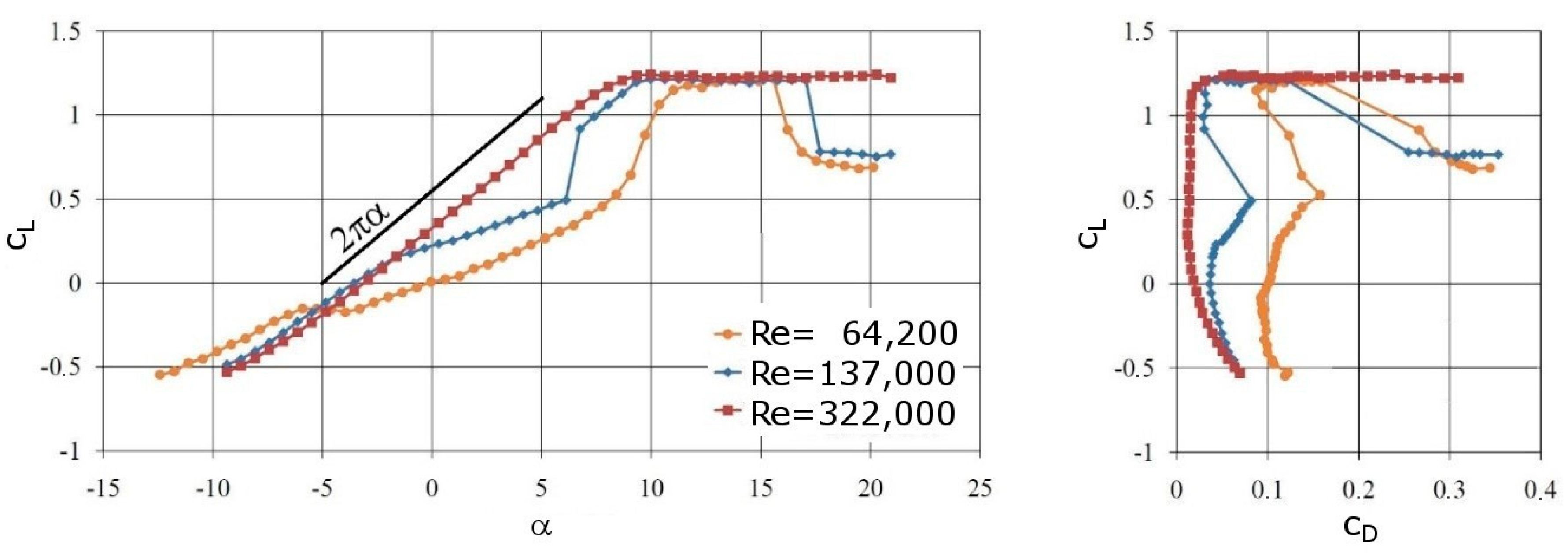
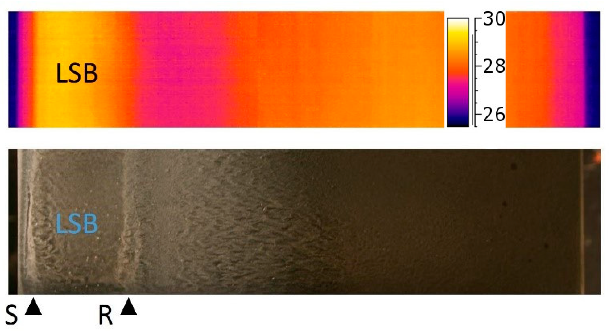
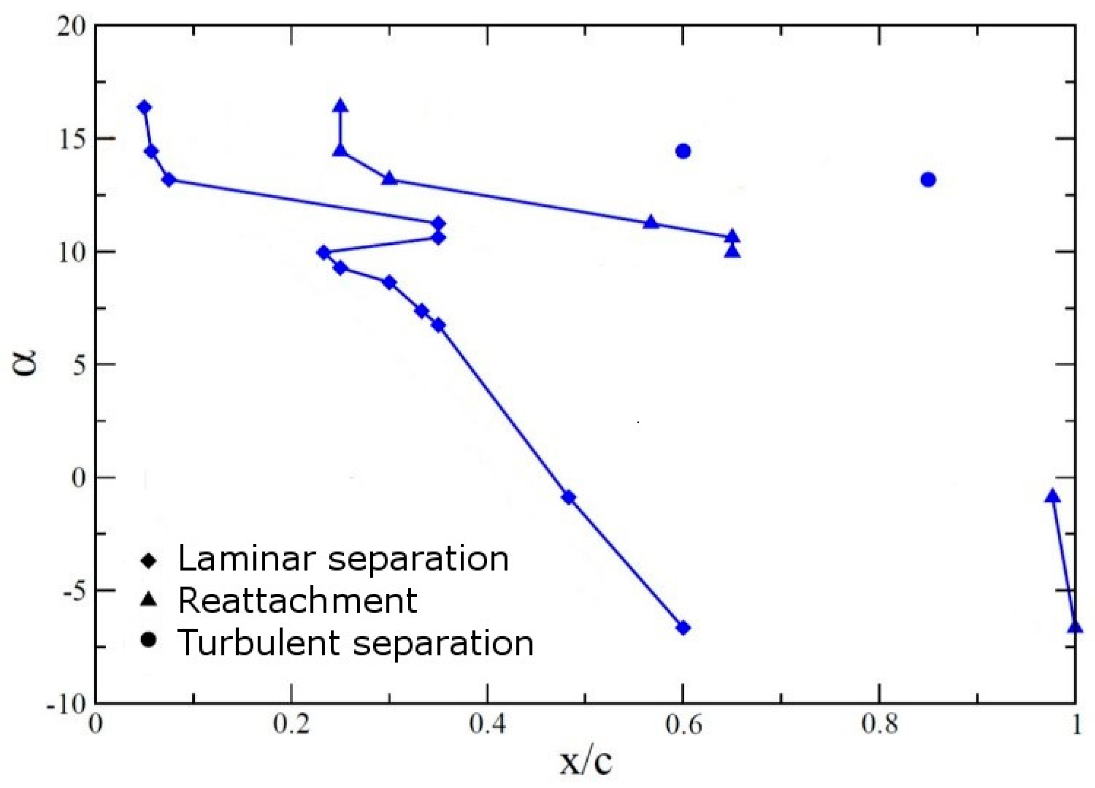
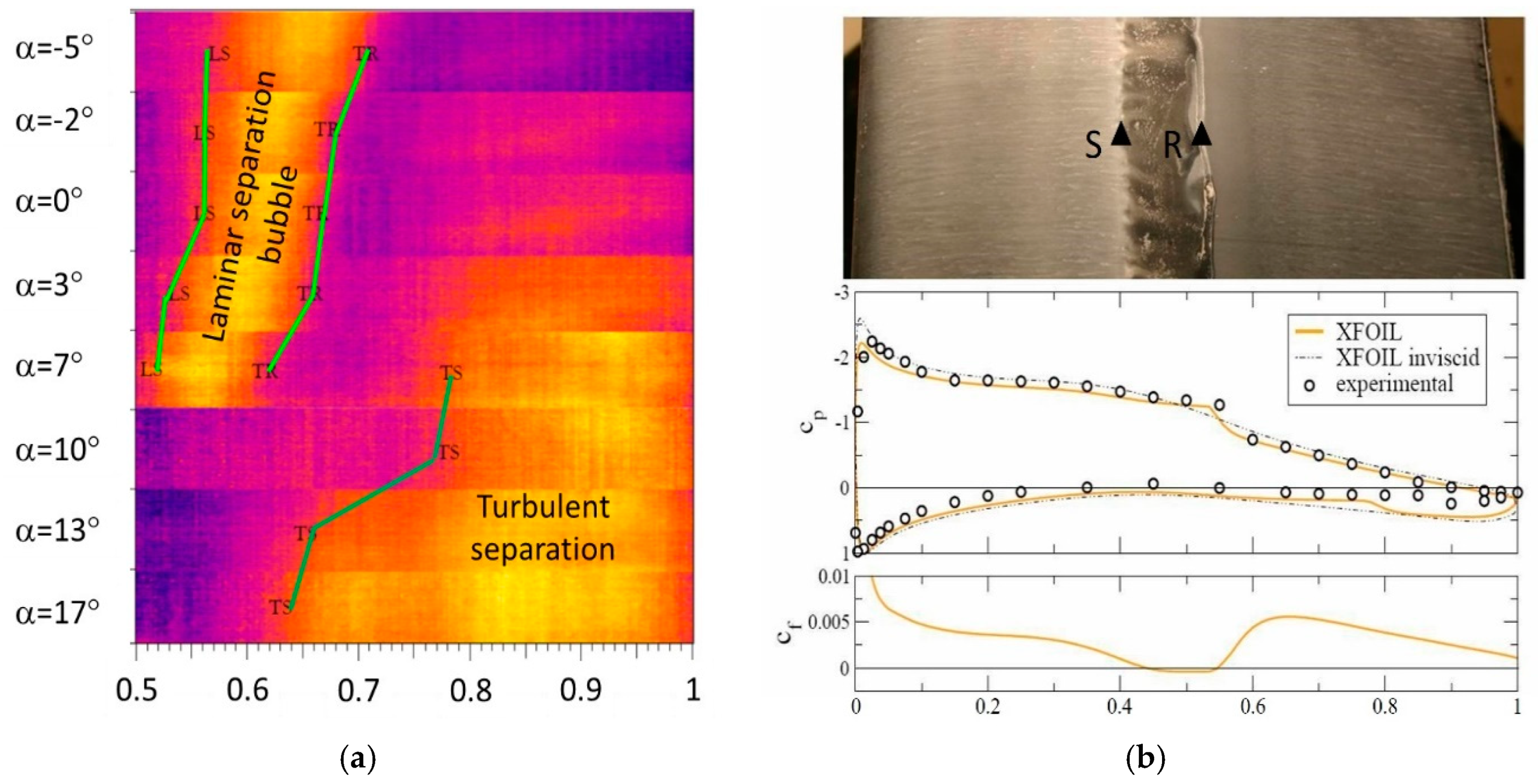
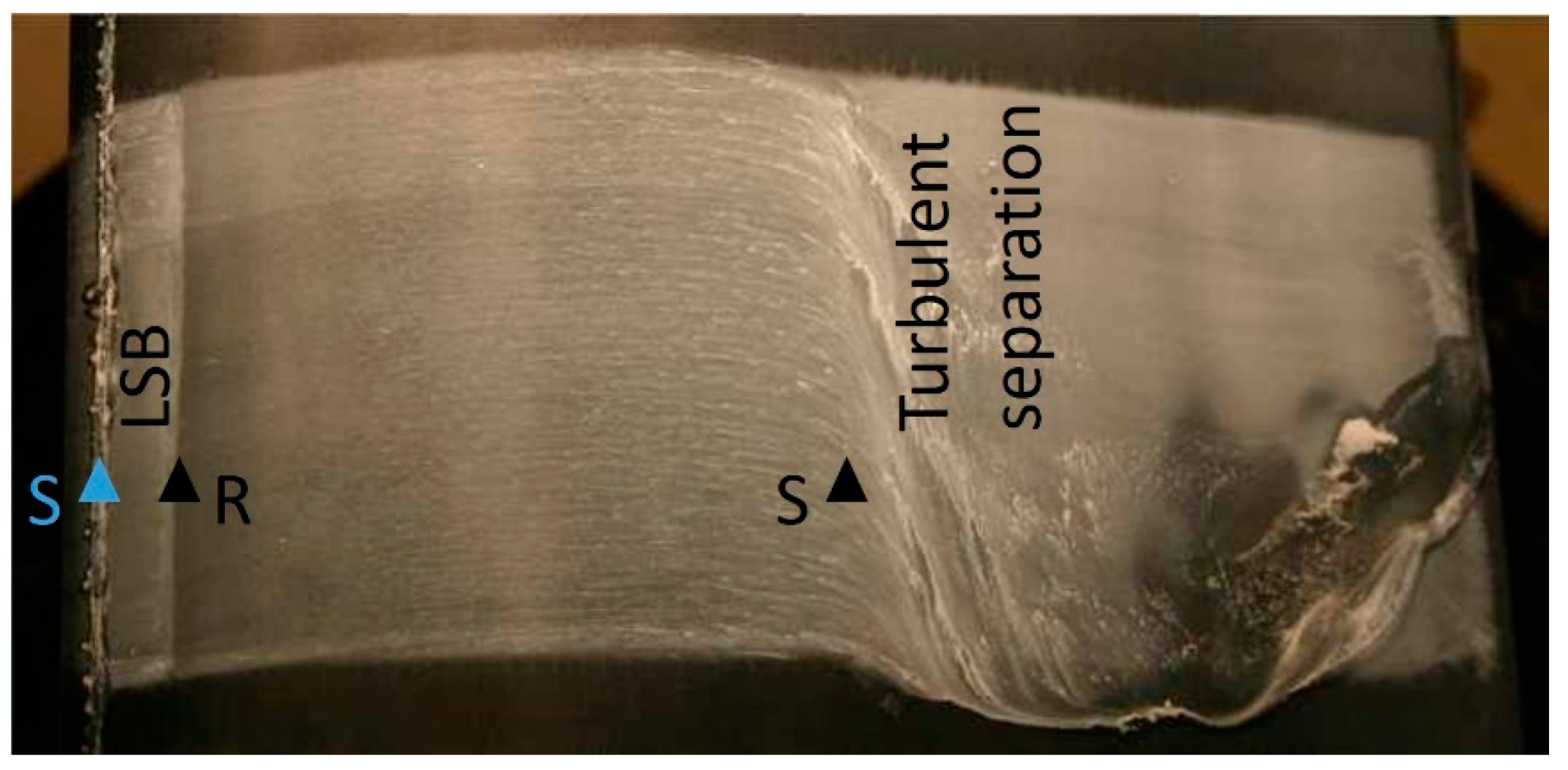
3.1. Wind Tunnel Investigation of Uncontrolled Flow

The wind tunnel experiments without AFC are discussed first, because they provide the baseline for the AFC investigations. The measured lift curves and drag polars for three Reynolds numbers are shown in Figure 13. Also included in the figure is the 2π lift curve slope from thin airfoil theory. For Re = 322,000 (based on MAC and airspeed of the 1:5 scale model during cruise), the measured lift curve slope is 2π up to α ≈ 7 degrees. For higher AoAs, the flow begins to separate turbulent from the trailing edge, and the airfoil stalls. As the Reynolds number is lowered to 137,000 (based on MAC and airspeed of 1:5 scale model at takeoff), the lift curve slope for −2 degrees < α < 5 degrees is reduced significantly, and the drag is increased, which is an indication of laminar separation. This effect becomes even more pronounced as the Reynolds number is further reduced to Re = 64,200 (based on the wing tip chord and airspeed of the 1:5 scale model at takeoff). Streamlines computed from time-averaged PIV data are shown in Figure 14. For α = 9 degrees, the flow separates laminar at about 30% chord (indicated by triangle and letter “S”), the lift is low, and the drag is high (Figure 13). As the AoA is increased past α = 10 degrees, the flow reattaches to the suction surface (Figure 14). Oil-flow and infrared images revealed that an LSB near the leading edge trips the suction-side boundary layer to turbulence (Figure 15). The turbulent boundary layer reattaches (letter “R”) to the suction surface, resulting in a lift recovery and a drag reduction (Figure 13). Since the skin friction in the recirculation region of the LSB is low, the surface is cooled less inside the bubble than in the reattachment region (high skin friction), and as a result, the wall temperature is higher (Figure 15). As the AoA is increased further, the suction-side boundary layer begins to separate turbulent from the trailing edge. At α = 16 degrees, the leading edge LSB opens up rapidly, leading to an abrupt loss of lift (“hard stall”, Figure 13). In the terminology of Gaster [3], the leading edge bubble is “bursting”.

A summary of the experimental results for Re = 64,200 is provided in Figure 16. As the AoA is increased from −7 degrees to 17 degrees, the laminar separation moves progressively upstream from 60% chord to about 4% chord. Around α ≈ 10 degrees, the separated boundary layer reattaches and forms an LSB. As a result, the laminar separation suddenly moves downstream from about 22% to about 37% of the chord. As the AoA is further increased, the LSB quickly shifts upstream toward the leading edge.

The same phenomena were also observed for Re = 137,000. At this more than two times larger Reynolds number, the laminar separation is less pronounced, and hence, the associated loss of lift and drag increase are more benign (Figure 13). The lift and drag data for Re = 322,000 (model cruise Reynolds number) show no noticeable non-linearity before stall (Figure 13), which suggests that the LSB is entirely missing. Surprisingly, the oil-flow and infrared imagery indicate the opposite. For example, Figure 17 shows an LSB near mid-chord (at the onset of the adverse gradient) for Re = 322,000 and α = 6.75 degrees. Included in Figure 17 are results obtained with the XFoil code by Drela [40]. Compared to Re = 64,200, the separated boundary layer transitions and reattaches more quickly, and as a result, the laminar bubble is short and shallow, and the effect on the lift and drag coefficient is negligible (Figure 13). As the AoA is increased, the LSB moves to the leading edge, and the flow begins to separate turbulent from the tailing edge. For example, for α = 13.2 degrees, the LSB is located at the leading edge, and the turbulent boundary layer separates at about 60% chord (Figure 18).

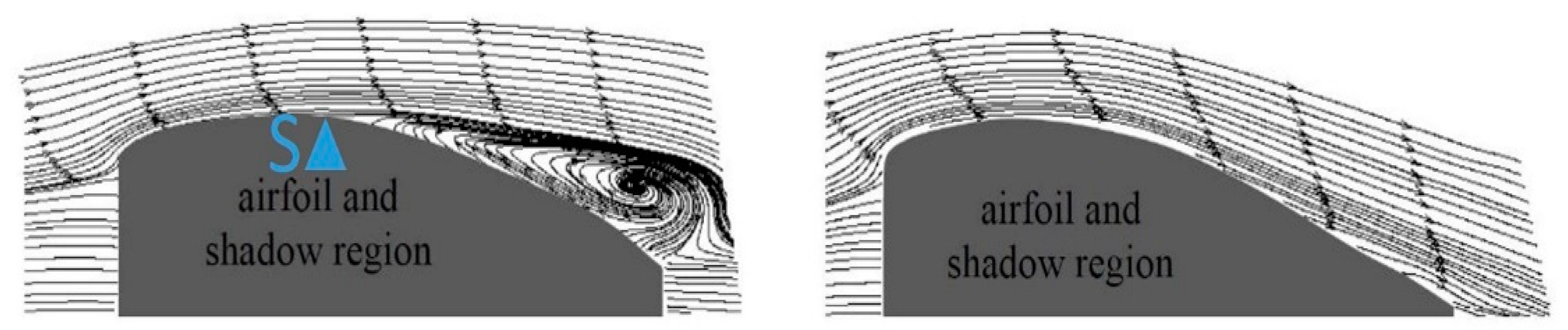
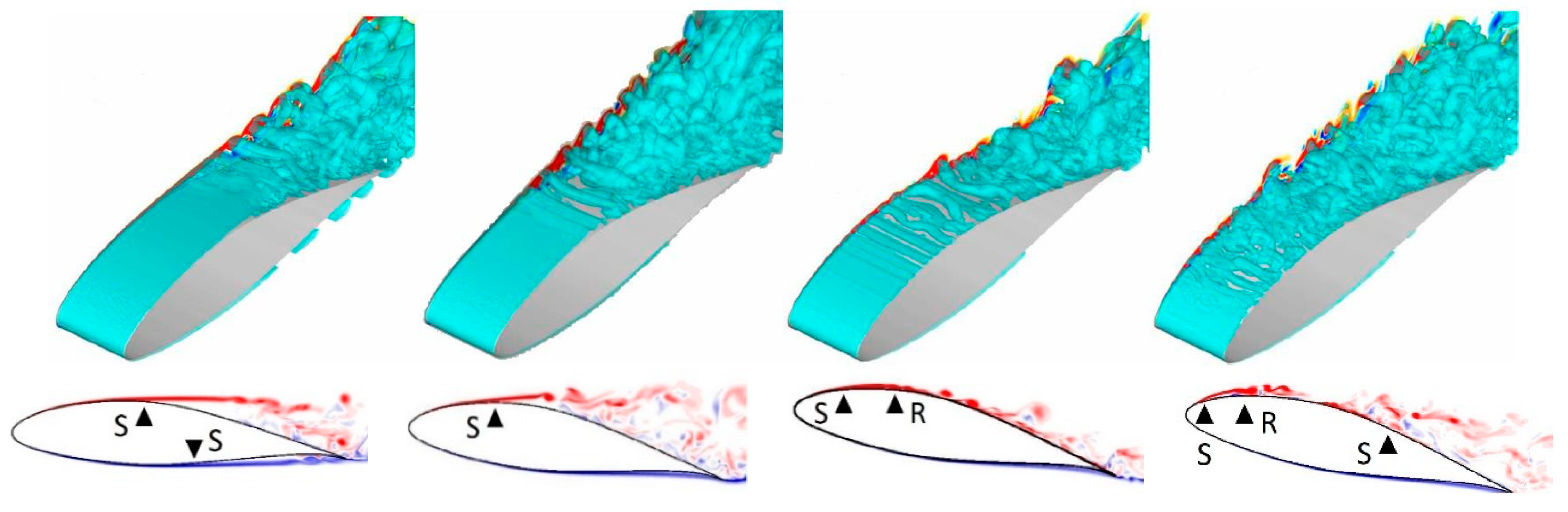
3.2. Simulations of Uncontrolled Flow

Extensive simulations were carried out for Re = 64,200 (based on wing tip chord and airspeed of the 1:5 scale model at takeoff). Since the laminar separation for this Reynolds number is more pronounced than at the higher Reynolds numbers, Re = 64,200 appeared to be well-suited for research aimed at investigations of the flow physics of LSC. Instantaneous flow visualizations obtained from simulations for Re = 64,200 and four different angles of attack are provided in Figure 19 (Brehm et al. [32]). Shown are isosurfaces of the Q vortex identification criterion by Hunt [41] and isocontours of the spanwise vorticity. For α = 4.19 degrees, the suction-side boundary layer separates laminar from the suction surface near 40% chord. As the AoA is increased to 8.64 degrees, the separation point moves upstream. For 11.24 degrees, the suction-side boundary layer reattaches turbulent, and an LSB is formed. As the AoA is increased further to 13.84 degrees, the LSB moves upstream toward the leading edge, and the turbulent boundary layer begins to separate from the trailing edge. The flow visualizations in Figure 19 reveal that the LSB is shedding spanwise coherent structures that are a likely consequence of Kelvin–Helmholtz (K-H) instability. These “primary” structures then become wavy in the spanwise direction before they break up into smaller random structures. This transition to turbulence is typical for LSBs in a low-disturbance environment (e.g., Balzer and Fasel [42]).

A comparison of the computed and measured wall pressure coefficient, c_p, distributions is provided in Figure 20. The general agreement between the simulations and wind tunnel measurements is quite good except for α = 11.24 degrees, where the LSB is shorter and farther upstream in the simulation (α = 11.24 degrees is close to the discontinuity in the data in Figure 16). As a result of the good agreement of the c_p-curves from the 3D simulations, the lift and drag data are also in decent agreement with the wind tunnel measurements by Mack et al. [28] (Figure 21).

Comparable well-resolved simulations at higher Reynolds numbers are computationally expensive. As an example, instantaneous flow visualizations from a simulation of the uncontrolled flow for Re = 300,000 and α = 15 degrees are provided in Figure 22. The flow topology is similar to that for Re = 64,200 and α = 13.84 degrees. A short and shallow leading edge LSB “trips” the suction-side boundary layer to turbulence. As shown by Benton and Visbal [1,2], a high-frequency 2D control of the LSB can delay the bursting of the LSB as the AoA is increased. Higher Reynolds number (300,000 and above) simulations are computationally expensive. Hybrid turbulence models that blend between LES and Reynolds-averaged Navier-Stokes (RANS) depending on the local physical grid resolution promise to be an attractive lower-cost alternative to ILES. Hybrid turbulence model simulations were carried out [33], but they did not capture the leading edge LSB, and thus were not appropriate for LSC research. Alternatively, to cut down on the computational expense, the geometry can be simplified. For example, Balzer and Fasel [42] carried out DNS of the suction surface at very high resolution. Wind tunnel and free-flight experiments appear more feasible for investigations at higher Reynolds numbers.

Included in Figure 21 are the lift and drag coefficient obtained from a 2D simulation for α = 8.64 degrees. Turbulence is artificially suppressed in the 2D simulation, and as a result, the spanwise coherent flow structures are overly strong compared to the 3D simulation (Figure 23a). For the 3D simulation, the spanwise structures quickly lose their coherence, and the flow does not reattach. For the 2D simulation, the strong spanwise coherent structures facilitate an effective wall normal momentum exchange, and the flow reattaches upstream of the leading edge (Figure 23b). As a result, the lift is increased, and the drag is lowered compared to the 3D simulation. This suggests that a control strategy that forces the 2D spanwise structures might be effective at suppressing laminar separation.

A local linear stability theory (LST) analysis of mean flow profiles (averaged in time and in the spanwise direction) that were spaced closely in the streamwise direction was carried out. In Figure 24a, the spatial growth rate, α_i, of the shear layer (K-H) mode is plotted as a function of the streamwise coordinate, s, (arc length over suction surface) and the reduced frequency, F⁺. When the frequency is held constant and the growth rate is integrated in s, an estimate for the expected flow response to a control that excites the K-H instability is obtained, $A\left(s\right)=A_{0}exp\left(-{{\displaystyle \int }}_{s_0}^s{\alpha }_{i}ds\right)$. In Figure 24b, the Fourier mode amplitudes of the skin friction coefficient (from the simulation) are compared with the expected flow response, $A\left(s\right)$, (from the LST) for various frequencies. The various curves are denoted by $\left(F^{+},k\right)$ where k is the spanwise mode number. The mode number is defined as $k=0.2/{\mathsf{\lambda }}_z$ where 0.2 is the spanwise domain extent, and ${\mathsf{\lambda }}_z$ is the spanwise wavelength of the Fourier modes (with λ_z = ∞ for the 2D mode, k = 0). The disturbance amplitudes obtained from the simulation for F⁺ = 1, 5, and 10 follow the LST results. This implies that the naturally occurring disturbances grow as a result of K-H instability.

3.3. Numerical Simulations of Controlled Flow

Strategies for the active laminar separation control (LSC) were investigated in wind tunnel, computer simulations, and free-flight experiments. The Reynolds number for most of the LSC research was 64,200. The simulations are discussed first. An efficient control is obtained when the control input is amplified by an underlying instability of the basic flow. In that case, the energy required for the disturbance amplification is drawn from the flow itself. Out of the frequencies that were selected for the analysis in Figure 24, the strongest disturbance amplification is observed for F⁺ = 5 and 10. The F⁺ = 5 mode obtained from the simulation saturates later than the F⁺ = 10 mode, and reaches a larger amplitude at mode saturation. For that reason, it was chosen for the AFC investigations.

A DBD plasma actuator was modeled by a volume force for the wall tangential velocity component. The volume force magnitude was 7.5 (non-dimensionalized by ${\rho }_{\infty }{v}_{\infty }^2/c$, where v_∞ is the free-stream velocity, and c is the chord length) and held constant over an area with streamwise and wall normal extent of 0.0056 × 0.0039 (normalized by chord length). The momentum coefficient was c_µ = 3.3 × 10⁻⁵. This model must be understood as a 2D volume forcing motivated by plasma actuators, and should not be confused with phenomenologically-derived plasma actuator models (e.g., Gaitonde et al. [12]). Pure 2D disturbances with a frequency of F⁺ = 5 were introduced near the leading edge at 2% chord with a reduced duty cycle of τ = 10% (Figure 25). The reduced duty cycle actuation introduces multiple harmonics [9]. For a nominal forcing frequency of five and a duty cycle of 10%, higher harmonics with frequencies of 10, 15, etc. are introduced at almost equal amplitude.

A comparison of the instantaneous uncontrolled and controlled flow in Figure 26 reveals that the control effectively suppresses separation. As a result, the lift is increased considerably, and the drag is lowered (

Table 2. Lift and drag coefficient. VGJs: vortex generator jets.

	cl	cd
Uncontrolled	0.654	0.121
2D volume forcing	1.26	0.0473
VGJs, B = 1	1.24	0.0465
VGJs, B = 4	1.12	0.0485

). Fourier mode amplitudes of the skin friction coefficient in Figure 27 reveal that the F⁺ = 5, 10, and 15 modes follow the LST results, and are growing by two to three orders of magnitude. This suggests that, as expected, the disturbance input is amplified as a result of the K-H instability. The F⁺ = 10 disturbance is amplified earlier than the F⁺ = 5 disturbance, and saturates earlier. Higher frequencies are amplified farther upstream, where the shear layer is thinner. This can also be seen in Figure 24a for the uncontrolled flow. Since disturbances for a broad range of frequencies are amplified strongly, the frequency chosen for an LSC approach does not need to exactly match the most amplified frequency. The frequency range that allows for an effective control depends on the forcing amplitude. Within limits, the larger the forcing amplitude, the larger the frequency range for which the control is effective. Figure 26 also reveals that with control, the spanwise coherent structures lose their coherence later than for the uncontrolled flow. Related research by Embacher and Fasel [43] showed that the onset of the secondary instability which leads to this loss of coherence (and transition to turbulence) can indeed be delayed through a 2D forcing at the proper frequency and amplitude. The ensuing laminar spanwise coherent structures were found to be very effective at delaying laminar separation. This mechanism was later exploited by Benton and Visbal [1,2] for delaying laminar separation from a wing section during a pitch-up maneuver. Hosseinverdi and Fasel [44] found that the transition delay was less pronounced in the presence of elevated free-stream turbulence.

Pulsed vortex generator jets (VGJs) are another common LSC strategy that can relatively easily be integrated into existing designs (e.g., Bons et al. [7], Postl et al. [8]). Pulsed VGJs with a spanwise spacing of 20% chord that were located at 26.7% chord were also considered in the simulations. The VGJ hole diameter was 2% of the chord length and the pitch and skew angle were 90 degrees and 30 degrees, respectively. The forcing frequency was F⁺ = 5, the duty cycle was τ = 10%, and the blowing ratio, B, was 1 and 4. The corresponding momentum coefficients were c_µ = 1.3 × 10⁻⁴ and 2.0 × 10⁻³. The VGJs were modeled by a velocity wall boundary condition. Instantaneous flow visualizations for the cases with pulsed VGJs (Figure 28) reveal no pronounced spanwise coherent structures as for the previous two cases. Nevertheless, for VGJs with B = 1, the mode (5,0) is still amplified by about 1.5 orders of magnitude before it saturates (Figure 29a). The B = 1 VGJs thus exploit the same physical mechanism as the 2D volume forcing AFC, i.e., they take advantage of the K-H instability (for a detailed discussion, see Postl and Fasel [8]). As a result, they are equally effective (Table 2). For B = 4, the mode amplitudes at the hole location are saturated, and no exponential disturbance growth is observed (Figure 29b). Interestingly though, a steady 3D mode, (0,1), is dominant downstream of the VGJs holes, and a visualization of the time-averaged flow field reveals that longitudinal vortices are generated (Figure 30; for clarity, the computational domain was repeated once in the spanwise direction). This finding is in agreement with PIV measurements by Hansen and Bons [45] for a flat plate boundary layer with adverse pressure gradient. The longitudinal vortices suppress separation through an increased wall-normal momentum exchange. However, the mechanism is less efficient, since it does not exploit an inherent flow instability, and is less effective than the control that exploits the 2D modes (Table 2).

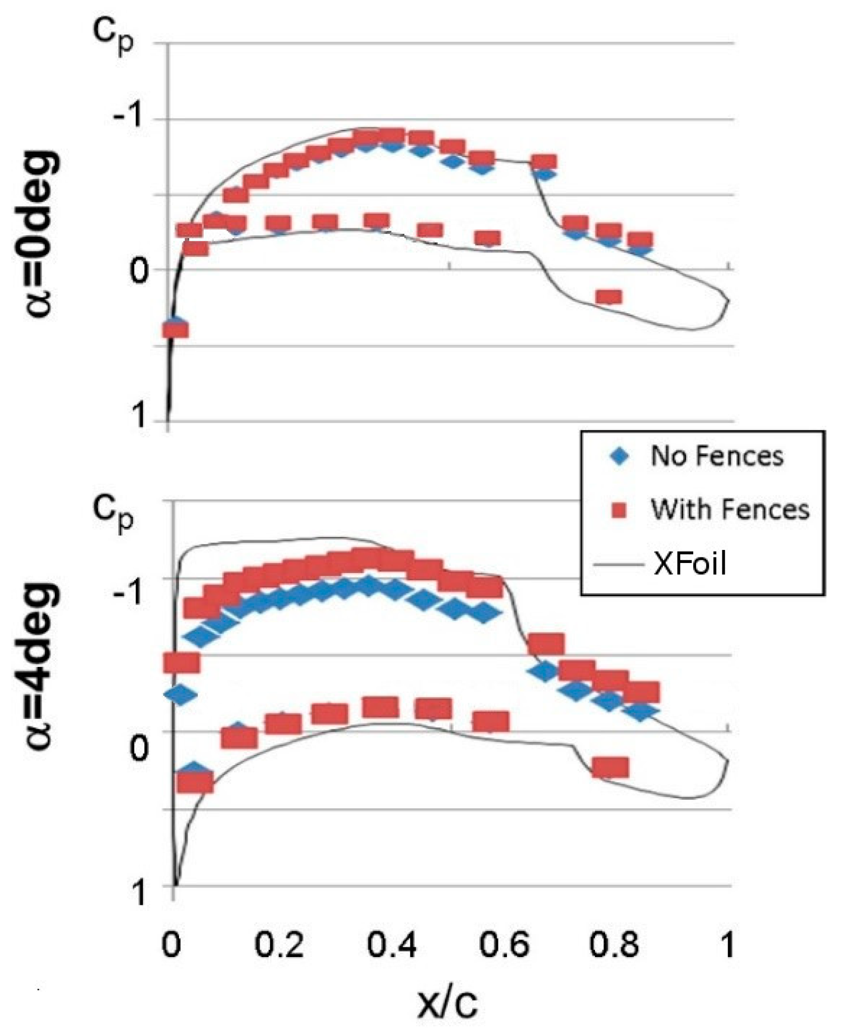
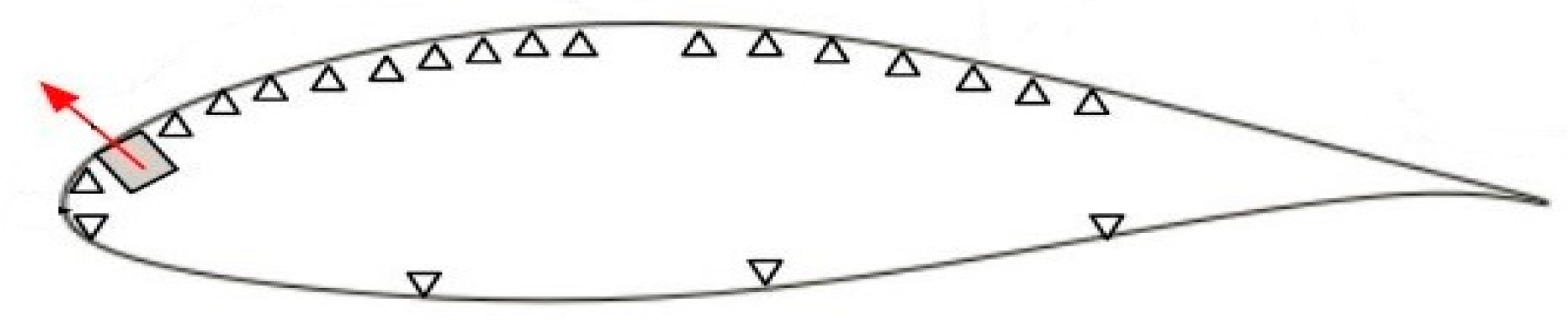
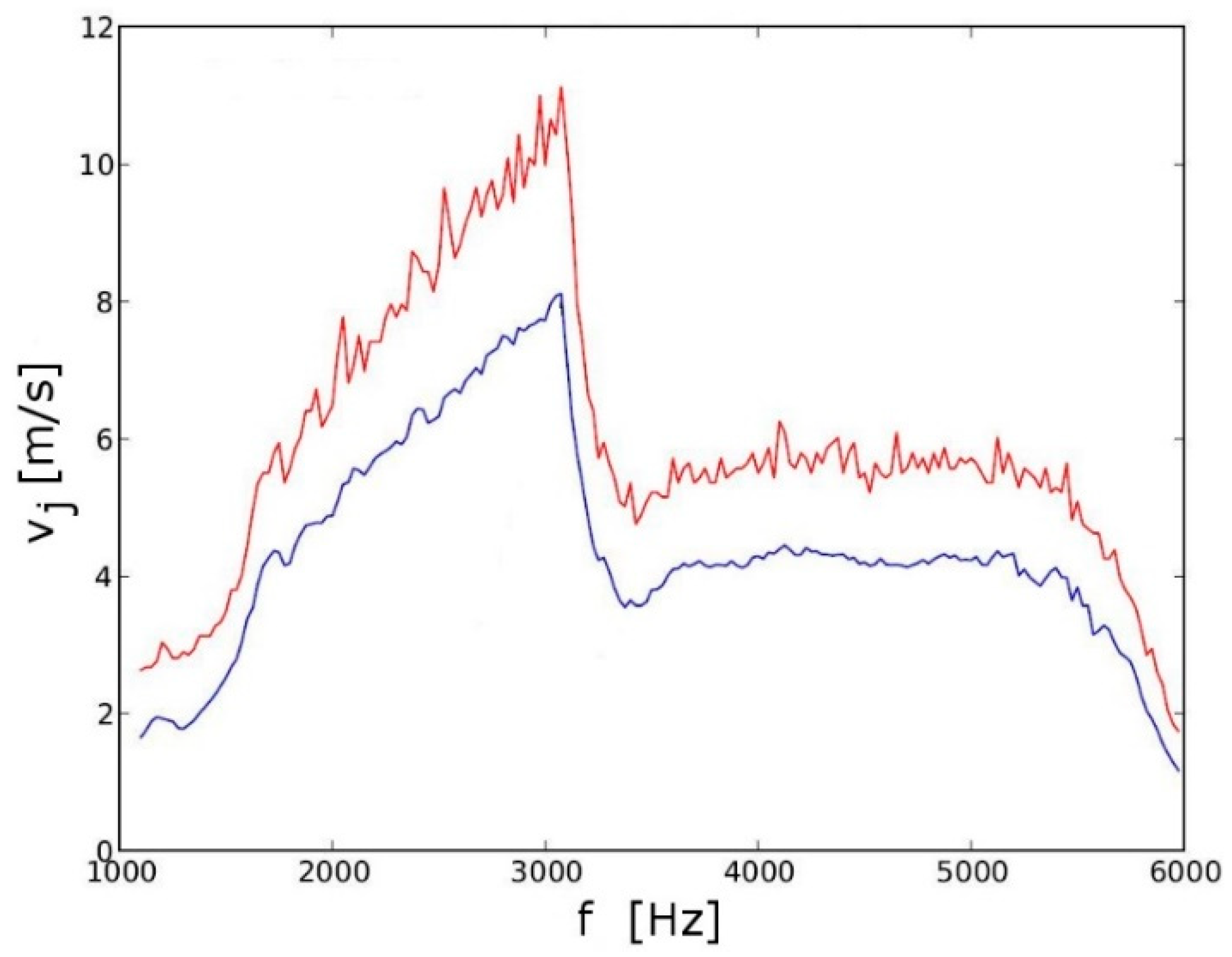
3.4. Wind Tunnel Investigations of Controlled Flow

In the wind tunnel experiments, 2D disturbances were introduced with DBD plasma actuators. A systematic investigation of the effect of the forcing frequency on the lift and drag coefficient was carried out for Re = 64,200. The plasma actuators were located at 2% and/or 40% chord. For α < 3 degrees, the flow separates downstream of 40% chord (Figure 16). When the actuator was placed at 40% chord, forcing frequencies in the range 2.63 < F⁺ < 6.14 (centered around F⁺ = 5 of simulations) effectively suppressed the laminar separation (Figure 31). For α = 8.7 degrees, the uncontrolled flow separates at 25% chord (Figure 32), and the flow topology is in agreement with the simulation for α = 8.64 degrees (Figure 19 and Figure 20). With control, the suction-side boundary is fully reattached (Figure 32; for simulation, see Figure 26). This result is surprising, as the actuator is located inside the separated flow region for the uncontrolled flow, which implies a significant damping of the forcing signal before it reaches the separated boundary layer. Due to the low DBD disturbance amplitude, this suggests a considerable disturbance amplification as a result of the K-H instability, as explained for the simulations. It must be speculated that the disturbance amplification by the K-H instability is large enough for the separated boundary layer to “pick up” the weakened forcing signal.

Since the passive (control off) actuator at 40% chord was found to “trip” the flow for −5 < α < 0 degrees (Figure 4), the AFC results for this AoA range are not meaningful. When the plasma actuator was placed at 2% chord in the favorable pressure gradient region, flow control with F⁺ = 4.38 was the most effective for an AoA range of −5 < α < 7 degrees (Figure 33). For this AoA range, the laminar separation is far downstream of the actuator location. Since disturbances are less amplified or even damped in favorable pressure gradient boundary layers, the disturbance amplitude at separation is smaller (than when the actuator is placed at 40% chord). When the disturbance amplitude is low, the effectiveness of the AFC becomes more frequency-dependent. Out of the chosen frequencies, the most effective lift recovery for −3 < α < −1 degrees is obtained with F⁺ = 4.38. For F⁺ = 0.88, a slight post-stall lift increase is observed for α >10 degrees (Figure 34). Post-stall AFC has to exploit coherent flow structures in the separated turbulent boundary layer. Turbulent separation control is not a subject of this article. Interestingly, for all of the forcing frequencies, stall is delayed from α ≈ 16 degrees to α ≈ 19 degrees. This suggests that the leading edge actuator prevents the bursting of the leading edge LSB.

Similar results were obtained for Re = 137,000 (Figure 35). For forcing frequencies between 0.82–7.40, a strong lift recovery is obtained for 0 degrees < α < 7 degrees. As for the lower Reynolds number case, the leading edge bubble bursting is suppressed, and the turbulent trailing edge separation (for α > 10 degrees) can be controlled with a low-frequency actuation (F⁺ = 0.82).

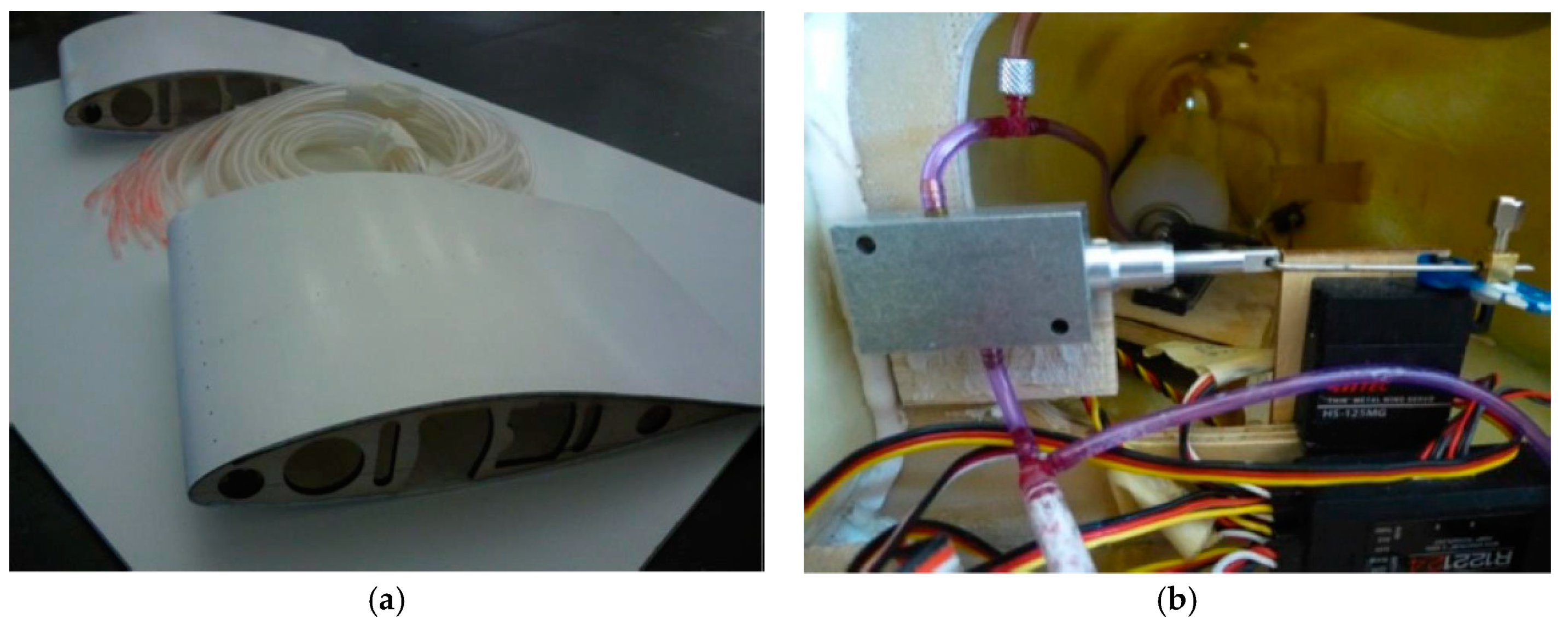
3.5. Wind Tunnel Experiments—Wing Glove

Finally, the free-flight experiments and the preparatory wind tunnel experiments are discussed. The wing gloves and all of the associated instrumentation were tested in the educational wind tunnel at the AME. This open return wind tunnel has a 31 cm (width and height) times 61 cm (length) test section, and a relatively high free-stream noise level (related to the fan motor frequency) that increases with tunnel speed. In Figure 36, wall pressure measurements and XFoil predictions are compared for a geometric angle of attack of α = 8.5 degrees. The overall poor quantitative agreement of the measurements and predictions can be explained by the large tunnel blockage of 18%, the low wing glove aspect ratio of 0.22/0.3 = 0.73 (which leads to 3D effects), and the high free-stream turbulence level (which affects laminar separation). For Re = 115,000 (close to model takeoff), a pressure plateau is observed near 50% chord, which is indicative of an LSB. For Re = 64,200, the measurement uncertainty is quite large (the Honeywell pressure sensor resolution is 3 Pa, and the relative error is 0.5%). Nevertheless, as in the wind tunnel experiments and simulations, a pressure plateau can be seen starting around 20–30% chord.

The actuators were also tested in the educational wind tunnel prior to flight. A reduced duty cycle actuation with τ = 50% was chosen and different Reynolds number, AoA, blowing ratio, and actuation frequency, F⁺, combinations were investigated. In Figure 37, Figure 38 and Figure 39, temporal Fourier transforms of the wall pressure coefficient are plotted versus the downstream coordinate for α = 8 degrees. The reduced duty cycle actuation introduces multiple higher harmonics [9]. In the figures, the nominal AFC frequency is marked by red arrows, and the first higher harmonic (if visible) is marked by orange arrows. As the Reynolds number is increased, the measurement uncertainty associated with the pressure transducers decreases, and the spectra become less noisy. The noise band near F⁺ = 1.75 for Re = 115,000 and F⁺ = 0.9 for Re = 280,000 could be traced back to the wind tunnel fan. For Re = 64,000 and B = 0.004, both the primary forcing frequency and its first higher harmonic are clearly visible, despite the high background noise level (Figure 37a). In qualitative agreement with the simulations (Figure 24b), the disturbances are amplified in the downstream direction. For B = 0.1, only the first higher harmonic is amplified, and the primary disturbance is missing (Figure 37b). A similar picture emerges for Re = 115,000 (Figure 38). For actuation with B = 0.002, the primary is amplified, and for B = 0.1, the first higher harmonic is amplified. For Re = 280,000, the fan noise frequency is at F⁺ = 0.9, and the flow control frequency was lowered to F⁺ = 0.5 and raised to F⁺ = 1.2 to allow for a clear separation of the flow control response from the fan noise (Figure 39). For Re = 280,000, the extent of the laminar separation is much reduced compared to Re = 64,000 (Figure 17), and it can be assumed that the disturbance amplification near 50% chord in Figure 39a was the result of an LSB.

3.6. Free-Flight Experiments—Wing Glove

Lift data from flight experiments with the first wing glove are shown in Figure 40. Also included in the same figure are two lift curves from the wind tunnel experiments (Figure 13). Since the flight data were obtained for a wide range of flight conditions (straight and level, accelerated/decelerated flight, different air speeds and Reynolds numbers, etc.) the data spread is large. Constant chord wing glove extensions as shown in Figure 12 were found to steepen the lift curve slope (i.e., increase the flow’s two-dimensionality). However, even with extensions, the lift curve slope is reduced compared to the wind tunnel experiments, and the maximum lift coefficient (at stall) is lowered. The dashed green and orange lines in Figure 40 indicate averages through the upper and lower half of the data that must be associated with the maximum and minimum flight speed during the flight testing. Both curves indicate stall near α ≈ 8 degrees.

In free-flight experiments, the AoA, α, side-slip angle, β, and airspeed, v, can change. Therefore, for each AFC experiment, only data from time series where α, β, and v were relatively constant were analyzed. Wall pressure distributions for Re = 390,000 and α = 0.3 degrees are compared in Figure 41. Without control, a pressure plateau is observed near 50% chord, which indicates an LSB. With control, the LSB is eliminated. Frequency spectra are provided in Figure 42. The forcing frequencies are marked by red arrows. For the uncontrolled case (Figure 42a), considerable low-frequency unsteadiness with F⁺ ≤ 0.07 (≈5 Hz) can be observed near reattachment (around 60% chord). For the cases with flow control, peaks in the spectra near 60% chord at the forcing frequency indicate that the AFC disturbances are amplified by the LSB. Overall, the disturbance levels are much lower than in the wind tunnel experiments (Figure 37, Figure 38 and Figure 39) due to the low free-stream turbulence intensity in the flight experiments.

Free-flight experiments were also carried out with the second wing glove, which featured surface-normal steady jets at 5% chord that could be activated via radio during flight. Wall pressure measurements that were obtained in free-flight experiments with the second wing glove at Re = 310,000 are presented in Figure 43. For the uncontrolled flow, in agreement with the XFoil prediction, a pressure plateau is observed near mid-chord. Steady blowing with B = 1.43 eliminates the laminar separation by transitioning the flow upstream of separation. The control is effective (i.e., it eliminates the LSB), but it is not efficient, since it requires a large blowing ratio. Laminar separation control by steady VGJs was investigated for example by Postl et al. [8,46]. Depending on the angle of the VGJ injection, one or two streamwise vortices are generated that entrain high-momentum free-stream fluid, thus suppressing separation.

4. Conclusions and Outlook

The physical understanding of laminar separation and its control is critically important for many applications, such as unmanned aerial vehicles and low-pressure turbines. A combined approach of numerical simulations, wind tunnel, and free-flight experiments was taken for investigating laminar separation and its control. An Aeromot 200S Super Ximango motor glider was chosen for the free-flight experiments, because it allows for long, low-disturbance power-off glides. The motor glider airfoil (modified NACA 64₃-618) was also used for the simulations and wind tunnel experiments. This laminar airfoil turned out to be ideal for investigating laminar separation and its control at low Reynolds number conditions. Wind tunnel experiments for Re = 64,200 revealed a large laminar separation that grows in size as the AoA is increased. Beyond a critical AoA, the boundary layer reattaches turbulent, and a laminar separation bubble (LSB) is formed. As the AoA is further increased, the LSB moves to the leading edge, and the flow begins to separate turbulent from the trailing edge. Dielectric barrier discharge (DBD) actuators were found to be highly effective at suppressing laminar separation. The high efficiency and effectiveness of the flow control was explained by the K-H instability of the separated boundary layer, which amplified the two-dimensional disturbance input. The effectiveness of the control was found to depend on the actuator location and the forcing frequency. The control was most effective when the disturbances were introduced directly upstream of separation, and the frequency was close to the most amplified frequency. Low-amplitude pulsed vortex generator jets (VGJs) were found to be equally effective and efficient, and exploit the same mechanism as the DBD actuator. High-amplitude VGJs introduce streamwise vortices that effectively suppress laminar separation. However, due to the large required blowing ratio, they are not efficient. Instrumented wing gloves were developed and built to validate these findings in free-flight experiments. Two wing gloves were flown on a 1:5 dynamically scaled model of the motor glider. Models are cheaper to operate, are a smaller loss in case of a crash than a full-size aircraft, and do not require a recertification when a wing glove is installed. The wing gloves were instrumented with commercial off-the-shelf pressure sensors and actuators. Customized electronic circuitry was developed for reading and recording the pressure signals as well as other relevant flight data, as well as for operating the actuators for the active flow control. The flight experiments also revealed strong disturbance amplification by the LSB. Although the low free-stream turbulence makes flight experiments desirable for investigating laminar separation and its control, they are challenging for many reasons. First, the airplane velocity, altitude, and attitude has to be maintained with high accuracy during the flight tests. All of the instrumentation has to be lightweight and small enough to fit inside the airplane. The unavoidable finite aspect ratio of the wing gloves leads to flow three-dimensionality at high angles of attack. Finally, the airspeed range is limited by the performance characteristics of the airplane. Some of these difficulties could be overcome. For example, with autopilot, the free-stream conditions during the flight experiments could be maintained more accurately. The wing glove finite aspect ratio problem could be avoided by using a high aspect ratio constant chord wing.

References

1. Benton, S.I.; Visbal, M.R. Investigation of High-Frequency Separation Control Mechanisms for Delay of Unsteady Separation. In Proceedings of the 8th AIAA Flow Control Conference, Washington, DC, USA, 13–17 June 2016. [Google Scholar] [CrossRef]
2. Benton, S.I.; Visbal, M.R. High-Frequency Forcing to Delay Dynamic Stall at Relevant Reynolds Number. In Proceedings of the 47th AIAA Fluid Dynamics Conference, Denver, CO, USA, 5–9 June 2017. [Google Scholar] [CrossRef]
3. Gaster, M. The Structure and Behavior of Laminar Separation Bubbles; AGARD CP 4; AGARD: Neuilly-sur-Seine, France, 1966; pp. 819–854. [Google Scholar]
4. Hain, R.; Kähler, C.J.; Radespiel, R. Dynamics of Laminar Separation Bubbles at Low-Reynolds-Number Aerofoils. J. Fluid Mech. 2009, 630, 129–153. [Google Scholar] [CrossRef]
5. Jones, L.E.; Sandberg, R.D.; Sandham, N.D. Direct Numerical Simulations of Forced and Unforced Separation Bubbles on an Airfoil at Incidence. J. Fluid Mech. 2008, 602, 175–207. [Google Scholar] [CrossRef]
6. Seifert, A.; Darabi, A.; Wygnanski, I. Delay of Airfoil Stall by Periodic Excitation. J. Aircr. 1996, 33, 691–698. [Google Scholar] [CrossRef]
7. Bons, J.P.; Sondergaard, R.; Rivir, R.B. Turbine Separation Control Using Pulsed Vortex Generator Jets. J. Turbomach. 2001, 123, 198–206. [Google Scholar] [CrossRef]
8. Postl, D.; Balzer, W.; Fasel, H.F. Control of laminar separation using pulsed vortex generator jets: Direct numerical simulations. J. Fluid Mech. 2011, 676, 81–109. [Google Scholar] [CrossRef]
9. Gross, A.; Balzer, W.; Fasel, H. Numerical Investigation of Low-Pressure Turbine Flow Control (Invited). In Proceedings of the 38th Fluid Dynamics Conference and Exhibit, Fluid Dynamics and Co-located Conferences, Seattle, WA, USA, 23–26 June 2008. [Google Scholar] [CrossRef]
10. Huang, J.; Corke, T.C.; Thomas, F.O. Plasma Actuators for Separation Control of Low-Pressure Turbine Blades. AIAA J. 2006, 44, 51–57. [Google Scholar] [CrossRef]
11. Huang, J.; Corke, T.C.; Thomas, F.O. Unsteady Plasma Actuators for Separation Control of Low-Pressure Turbine Blades. AIAA J. 2006, 44, 1477–1487. [Google Scholar] [CrossRef]
12. Gaitonde, D.V.; Visbal, M.R.; Roy, S. Control of Flow Past a Wing Section with Plasma-Based Body Forces. In Proceedings of the 36th AIAA Plasmadynamics and Lasers Conference, Toronto, ON, Canada, 6–9 June 2005. [Google Scholar] [CrossRef]
13. Rizzetta, D.P.; Visbal, M.R. Numerical Investigation of Plasma-Based Flow Control for a Transitional Highly-Loaded Low-Pressure Turbine. AIAA J. 2007, 45, 2554–2564. [Google Scholar] [CrossRef]
14. Visbal, M.R.; Gaitonde, D.V.; Roy, S. Control of Transitional and Turbulent Flows Using Plasma-Based Actuators. In Proceedings of the 36th AIAA Fluid Dynamics Conference and Exhibit, San Francisco, CA, USA, 5–8 June 2006. [Google Scholar] [CrossRef]
15. Cain, A.B.; Ng, T.T.; Kerschen, E.J.; Fasel, H.F.; Fasse, E.D.; Israel, D.M. Flight Demonstration of Stealthy Closed-Loop Attitude Control; AFOSR STTR Final Report Contract FA49620-01-C-0044; Defense Technical Information Center: Fort Belvoir, VA, USA, 2002. [Google Scholar]
16. Ciuryla, M.; Liu, Y.; Farnsworth, J.; Kwan, C.; Amitay, M. Flight Control Using Synthetic Jets on a Cessna 182 Model. J. Aircr. 2007, 44, 642–653. [Google Scholar] [CrossRef]
17. Seifert, A.; David, S.; Fono, I.; Stalnov, O.; Dayan, I. Roll Control via Active Flow Control: From Concept to Flight. J. Aircr. 2010, 47, 864–874. [Google Scholar] [CrossRef]
18. Braslow, A.L. A History of Suction-Type Laminar-Flow Control with Empahsis on Flight Research; NASA History Division, Monographs in Aerospace History: Washington, DC, USA, 1999. [Google Scholar]
19. Nitsche, W.; Suttan, J.; Becker, S.; Erb, P.; Kloker, M.; Stemmer, C. Experimental and numerical investigations of controlled transition in low-speed free flight. Aerosp. Sci. Technol. 2001, 5, 245–255. [Google Scholar] [CrossRef]
20. Duchmann, A.; Simon, B.; Tropea, C.; Grundmann, S. Dielectric Barrier Discharge Plasma Actuators for In-Flight Transition Delay. AIAA J. 2014, 52, 358–367. [Google Scholar] [CrossRef]
21. Peltzer, I.; Pätzold, A.; Nitsche, W. In-Flight Experiments on Delaying Laminar-Turbulent Transition on a Laminar Wing Glove. J. Aerosp. Eng. 2009, 223, 619–626. [Google Scholar] [CrossRef]
22. Peltzer, I.; Wicke, K.; Pätzold, A.; Nitsche, W. In-flight experiments on active TS-wave control on a 2D-laminar wing glove. In Seventh IUTAM Symposium on Laminar-Turbulent Transition; IUTAM Bookseries; Schlatter, P., Henningson, D., Eds.; Springer: Dordrecht, The Netherland, 2010; Volume 18. [Google Scholar]
23. Belisle, M.; Roberts, M.; Williams, T.; Tufts, M.; Tucker, A.; Saric, W.; Reed, H. A Transonic Laminar-Flow Wing Glove Flight Experiment: Overview and Design Optimization. In Proceedings of the 30th AIAA Applied Aerodynamics Conference, New Orleans, LA, USA, 25–28 June 2012. [Google Scholar] [CrossRef]
24. Gross, A.; Pearman, C.; Kremer, R.; Napier, B.; Gosla, C.; Kurz, A.; Mack, S.; Brehm, C.; Heine, B.; Radi, A.; et al. 1/5 Scale Model of Aeromot 200S SuperXimango for Scaled Flight Research. In Proceedings of the 26th AIAA Applied Aerodynamics Conference, Honolulu, HI, USA, 18–21 August 2008. [Google Scholar] [CrossRef]
25. Wolowicz, C.H.; Bowman, J.S.; Gilbert, W.P. Similitude Requirements and Scaling Relationships as Applied to Model Testing; NASA TP-1435; NASA Langley Research Center: Hampton, VA, USA, 1979.
26. Gainer, T.G.; Hoffman, S. Summary of Transformation Equations and Equations of Motion Used in Free-Flight and Wind Tunnel Data Reduction and Analysis; NASA SP-3070; NASA Langley Research Center: Hampton, VA, USA, 1972.
27. Jordan, T.; Foster, J.; Bailey, R.; Belcastro, C. AirSTAR: A UAV Platform for Flight Dynamics and Control System Testing. In Proceedings of the 25th AIAA Aerodynamic Measurement Technology and Ground Testing Conference, San Francisco, CA, USA, 5–8 June2006. [Google Scholar] [CrossRef]
28. Mack, S.; Brehm, C.; Heine, B.; Fasel, H. Experimental Investigation of Separation and Separation Control of a Laminar Airfoil. In Proceedings of the 4th Flow Control Conference, Seattle, WA, USA, 23–26 June 2008. [Google Scholar] [CrossRef]
29. Plogmann, B.; Mack, S.; Fasel, H.F. Experimental Investigation of Open- and Closed-Loop Control for Airfoil under Low Reynolds Number Conditions. In Proceedings of the 39th AIAA Fluid Dynamics Conference, San Antonio, TX, USA, 22–25 June 2009. [Google Scholar] [CrossRef]
30. Gross, A.; Fasel, H.F. High-Order-Accurate Numerical Method for Complex Flows. AIAA J. 2008, 46, 204–214. [Google Scholar] [CrossRef]
31. Gross, A.; Fasel, H.F. Active Flow Control for NACA 6-Series Airfoil at Re = 64,200. AIAA J. 2010, 48, 1889–1902. [Google Scholar] [CrossRef]
32. Brehm, C.; Mack, S.; Gross, A.; Fasel, H.F. Investigations of an Airfoil at Low Reynolds Number Conditions. In Proceedings of the 4th Flow Control Conference, Seattle, WA, USA, 23–26 June 2008. [Google Scholar] [CrossRef]
33. Gross, A.; Fasel, H.F. Hybrid Turbulence Model Simulations of Partially Stalled Airfoil Flow. AIAA J. 2016, 54, 1220–1234. [Google Scholar] [CrossRef]
34. Margolin, L.G.; Rider, W.J. A rationale for implicit turbulence modeling. Int. J. Num. Meth. Fluids 2002, 39, 821–841. [Google Scholar] [CrossRef]
35. Visbal, M.R.; Garmann, D.J. Numerical Investigation of Spanwise End Effects on Dynamic Stall of a Pitching NACA 0012 Wing. In Proceedings of the 55th AIAA Aerospace Sciences Meeting, Grapevine, TX, USA, 9–13 January 2017. [Google Scholar] [CrossRef]
36. Broeren, A.P.; Bragg, M.B. Spanwise Variation in the Unsteady Stalling Flowfields of Two-Dimensional Airfoil Models. AIAA J. 2001, 39, 1641–1651. [Google Scholar] [CrossRef]
37. Dianics, J.V.; Balthazar, M.A.; Gross, A.; Fasel, H.F. Wind Tunnel and Free-Flight Testing of Active Flow Control for Modified NACA 643-618 Airfoil. In Proceedings of the 31st AIAA Applied Aerodynamics Conference, San Diego, CA, USA, 24–27 June 2013. [Google Scholar] [CrossRef]
38. Dianics, J.V.; Ohno, D.M.; Fuggmann, S.D.; Lay, J.; Heim, D.; Fasel, H.F. Numerical and Experimental Wind Tunnel and Flight Testing of Active Flow Control for Modified NACA 643-618 Airfoil. In Proceedings of the 53rd AIAA Aerospace Sciences Meeting, Kissimmee, FL, USA, 5–9 January 2015. [Google Scholar] [CrossRef]
39. Sinclair, A.R.; Robins, A.W. A Method for the Determination of the Time Lag in Pressure Measuring Systems Incorporating Capillaries; NACA TN 2793; NASA Langley Research Center: Hampton, VA, USA, 1952.
40. Drela, M.; Giles, M.B. Viscous-inviscid analysis of transonic and low Reynolds number airfoils. AIAA J. 1987, 25, 1347–1355. [Google Scholar] [CrossRef] [Green Version]
41. Hunt, J.C.R.; Wray, A.A.; Moin, P. Eddies, Stream, and Convergence Zones in Turbulent Flows; Report CTR-S88; Center for Turbulence Research: Stanford, CA, USA, 1988. [Google Scholar]
42. Balzer, W.; Fasel, H.F. Direct Numerical Simulation of Laminar Boundary-Layer Separation and Separation Control on the Suction Side of an Airfoil at Low Reynolds Number Conditions. In Proceedings of the 40th Fluid Dynamics Conference and Exhibit, Chicago, IL, USA, 28 June–1 July 2010. [Google Scholar] [CrossRef]
43. Embacher, M.; Fasel, H.F. Direct numerical simulations of laminar separation bubbles: Investigation of absolute instability and active flow control of transition to turbulence. J. Fluid Mech. 2014, 747, 141–185. [Google Scholar] [CrossRef]
44. Hosseinverdi, S.; Fasel, H.F. Numerical Investigation of the Interaction of Active Flow Control and Klebanoff Modes. In Proceedings of the 47th AIAA Fluid Dynamics Conference, Denver, CO, USA, 5–9 June 2017. [Google Scholar] [CrossRef]
45. Hansen, L.; Bons, J. Flow Measurements of Vortex Generator Jets in Separating Boundary Layer. J. Prop. Power 2006, 22, 558–566. [Google Scholar] [CrossRef]
46. Postl, D. Numerical Investigation of Laminar Separation Control Using Vortex Generator Jets. Ph.D. Dissertation, University of Arizona, Tucson, AZ, USA, 2005. [Google Scholar]
Figure 1. (a) Full-size and 1:5 scale AMT 200S. (b) 1:5 model in flight.
Aerospace 05 00114 g001
Figure 2. Model instrumentation.
Aerospace 05 00114 g002
Figure 3. (a) Wide and (b) narrow fiberglass wing. (Reprinted from [28,29]).
Aerospace 05 00114 g003
Figure 4. Upstream and downstream facing (deactivated) plasma actuator at 40% chord and plain wing without plasma actuator for Re = 64,200. (Reprinted from [28]).
Aerospace 05 00114 g004
Figure 5. Harmonic amplitude modulation of carrier signal.
Aerospace 05 00114 g005
Figure 6. Computational grid for (a) Re = 64,200 and (b) Re = 300,000 simulation (every fourth grid line is shown). (Reprinted from [31,33]).
Aerospace 05 00114 g006
Figure 7. CAD design of wing glove. (Reprinted by permission of the American Institute of Aeronautics and Astronautics, Inc. (Reston, VA, USA) from [37]).
Aerospace 05 00114 g007
Figure 8. Wall pressure measurements and XFoil predictions for Re = 320,000, α = 0 degrees (top) and α = 4 degrees (bottom).
Aerospace 05 00114 g008
Figure 9. Wing-glove schematic with pressure tap (triangles) and actuator locations (square). (Reprinted by permission of the American Institute of Aeronautics and Astronautics, Inc. (Reston, VA, USA) from [37]).
Aerospace 05 00114 g009
Figure 10. Dependence of jet velocity, vj, on carrier frequency, f. Red is maximum jet velocity; blue is mean jet velocity. (Reprinted by permission of the American Institute of Aeronautics and Astronautics, Inc. (Reston, VA, USA) from [37]).
Aerospace 05 00114 g010
Figure 11. (a) Second instrumented wing glove and dummy. (b) Air tank and pressure regulator. (Reprinted from [38]).
Aerospace 05 00114 g011
Figure 12. Wing glove with fences and constant chord extension. (Reprinted by permission of the American Institute of Aeronautics and Astronautics, Inc. (Reston, VA, USA) from [37]).
Aerospace 05 00114 g012
Figure 13. Lift curves and 2π slope of thin airfoil theory as well as drag polars. (Reprinted from [29]).
Aerospace 05 00114 g013
Figure 14. Mean-flow streamlines for Re = 64,200 and α = 9 degrees (left), 12.9 degrees (right). (Reprinted from [29]).
Aerospace 05 00114 g014
Figure 15. Infrared image (top, temperature scale in degrees Celsius) and oil-flow visualization (bottom) for Re = 64,200 and α = 13.5 degrees. (Reprinted from [29]).
Aerospace 05 00114 g015
Figure 16. Separation and reattachment locations as function of angle of attack (AoA). (Reprinted from [28]).
Aerospace 05 00114 g016
Figure 17. Re = 322,000: (a) Infrared imagery (similar temperature scale as in Figure 15) and (b) oil-flow visualization, wall pressure coefficient, and skin friction coefficient for α = 6.75 degrees.
Aerospace 05 00114 g017
Figure 18. Oil-flow visualization for Re = 322,000 and α = 13.2 degrees.
Aerospace 05 00114 g018
Figure 19. Instantaneous flow visualizations of Q = 100 and spanwise vorticity (−100 < ωz < 100) with mean separation (S) and reattachment (R) for Re = 64,200 and α = 4.19 degrees, 8.64 degrees, 11.24 degrees, and 13.84 degrees (left to right). (Reprinted from [32]).
Aerospace 05 00114 g019
Figure 20. Computed (lines) and measured (symbols) wall pressure coefficient distributions for Re = 64,200 and (a) α = 4.19 degrees, (b) 8.64 degrees, (c) 11.24 degrees, and (d) 13.84 degrees. (Reprinted from [28]).
Aerospace 05 00114 g020
Figure 21. Lift and drag data for Re = 64,200. (Reprinted from [32]).
Aerospace 05 00114 g021
Figure 22. Re = 300,000 and α = 15 degrees. (a) Instantaneous Q = 100 surfaces and (b) wall pressure and skin-friction coefficient. (Reprinted from [33]).
Aerospace 05 00114 g022
Figure 23. (a) Instantaneous visualizations of spanwise vorticity (−100 < ωz < 100) and (b) streamfunction isocontours computed from temporal averages (2D: dashed lines, 3D: solid lines, spanwise average) for Re = 64,200 and α = 8.64 degrees (Reprinted from [32]).
Aerospace 05 00114 g023
Figure 24. (a) Spatial growth rate (Reprinted from [31]) and (b) suction surface skin friction coefficient Fourier amplitudes (dashed lines: linear stability theory (LST), solid lines: simulation).
Aerospace 05 00114 g024
Figure 25. Reduced duty cycle actuation.
Aerospace 05 00114 g025
Figure 26. Re = 64,200 and α = 8.64 degrees: (Top) Isosurfaces of Q = 1 and isocontours of spanwise vorticity (−100 < ωz < 100). (Bottom) Suction-surface skin friction (−0.01 < cf < 0.01). Uncontrolled (left) and 2D volume forcing (right). (Reprinted from [31]).
Aerospace 05 00114 g026
Figure 27. Top surface skin friction coefficient Fourier amplitudes for 2D volume forcing (dashed lines: LST, solid lines: simulation).
Aerospace 05 00114 g027
Figure 28. Re = 64,200 and α = 8.64 degrees: (Top) Isosurfaces of Q = 1 and isocontours of spanwise vorticity (−100 < ωz < 100). (Bottom) Suction surface skin friction (−0.01 < cf < 0.01). Pulsed VGJs with B = 1 (left) and B = 4 (right). (Reprinted from [31]).
Aerospace 05 00114 g028
Figure 29. Top surface skin friction coefficient Fourier amplitudes (dashed lines: LST, solid lines: simulation) for pulsed VGJs with (a) B = 1 and (b) B = 4.
Aerospace 05 00114 g029
Figure 30. Isosurfaces of Q = 10, streamwise vorticity, ωx = −10, 10, and isocontours of velocity magnitude computed from time-average for pulsed VGJs with B = 4. (Reprinted from [31]).
Aerospace 05 00114 g030
Figure 31. Lift curve and drag polar for Re = 64,200. Plasma actuator at 40% chord. (Reprinted from [29]).
Aerospace 05 00114 g031
Figure 32. Mean-flow streamlines for Re = 64,200 and α = 8.7 degrees. (a) Uncontrolled flow and (b) plasma actuator at 40% chord with F+ = 4.38. (Reprinted from [29]).
Aerospace 05 00114 g032
Figure 33. Lift curve and drag polar for Re = 64,200. Plasma actuator at 2% chord. (Reprinted from [29]).
Aerospace 05 00114 g033
Figure 34. Mean-flow streamlines for Re = 64,200 and α = 13.8 degrees. (a) Uncontrolled flow and (b) plasma actuator at 2% chord with F+ = 0.88. (Reprinted from [29]).
Aerospace 05 00114 g034
Figure 35. Lift curve and drag polar for Re = 137,000. Plasma actuator at 2% chord. (Reprinted from [29]).
Aerospace 05 00114 g035
Figure 36. Wall pressure coefficient measurements (large circles: averages, small circles: uncertainty) and XFoil predictions (solid line) for α = 8.5 degrees and (a) Re = 115,000 and (b) Re = 64,200. (Reprinted by permission of the American Institute of Aeronautics and Astronautics, Inc. (Reston, VA, USA) from [37]).
Aerospace 05 00114 g036
Figure 37. Wing glove wind tunnel measurements for Re = 64,000 and α = 8 degrees. Temporal Fourier transforms of wall pressure coefficient versus chord length. Active flow control with F+ = 1.1 and (a) B = 0.004 and (b) B = 0.1. (Reprinted by permission of the American Institute of Aeronautics and Astronautics, Inc. (Reston, VA, USA) from [37]).
Aerospace 05 00114 g037
Figure 38. Wing glove wind tunnel measurements for Re = 115,000 and α = 8 degrees. Temporal Fourier transforms of wall pressure coefficient versus chord length. Active flow control with F+ = 1.0 and (a) B = 0.002 and (b) B = 0.1. (Reprinted by permission of the American Institute of Aeronautics and Astronautics, Inc. (Reston, VA, USA) from [37]).
Aerospace 05 00114 g038
Figure 39. Wing glove wind tunnel measurements for Re = 280,000 and α = 8 degrees. Temporal Fourier transforms of wall pressure coefficient versus chord length. Active flow control with B = 0.81 and (a) F+ = 0.46 and (b) F+ = 1.2. (Reprinted by permission of the American Institute of Aeronautics and Astronautics, Inc. (Reston, VA, USA) from [37]).
Aerospace 05 00114 g039
Figure 40. Lift coefficient data from flight tests (symbols; reprinted by permission of the American Institute of Aeronautics and Astronautics, Inc. (Reston, VA, USA) from [37]) superimposed with curve fits for minima and maxima with extensions and wind tunnel lift curves for Re = 137,000 and 322,000.
Aerospace 05 00114 g040
Figure 41. Free-flight measurements for Re = 390,000 and α = 0.3 degrees. Black symbols: Uncontrolled flow. Red symbols: F+ = 1.05 and B = 0.05. Blue symbols: F+ = 0.75 and B = 0.05. Solid line: XFoil. (Reprinted by permission of the American Institute of Aeronautics and Astronautics, Inc. (Reston, VA, USA) from [37]).
Aerospace 05 00114 g041
Figure 42. Free-flight measurements for Re = 390,000 and α = 0.3 degrees. Wall pressure coefficient spectra. (a) Uncontrolled, (b) control with F+ = 0.75 and B = 0.05, and (c) control with F+ = 1.05 and B = 0.05 (Reprinted by permission of the American Institute of Aeronautics and Astronautics, Inc. (Reston, VA, USA) from [37]).
Aerospace 05 00114 g042
Figure 43. Measured and predicted (XFoil) wall pressure coefficient distributions for Re = 310,000 and α = 0 degrees. (a) Uncontrolled flow and (b) steady blowing with B = 1.43. (Reprinted from [38]).
Aerospace 05 00114 g043