The Development of an Ordinary Least Squares Parametric Model to Estimate the Cost Per Flying Hour of ‘Unknown’ Aircraft Types and a Comparative Application †


Abstract
1. Introduction
- The proportional CPFH model works: When nothing changes in the way an aircraft fleet flies (and rests) from one period to the next. It is then perfectly reasonable to use flying hours as a predictor for removal-causing failures. When fight behaviour does not change, the failure rate from each potential cause of failures remains constant.
- The proportional CPFH model fails: When a fleet of aircraft significantly changes its flight behaviour from one time interval to the next. An example of this is the wartime surge (flying hours increase dramatically but landings remain the same) and this is a typical case in which flying hours and the other factors that affect failures begin to diverge.
2. Materials and Methods
2.1. The Parametric Estimation Technique
Parametric estimating is a technique that develops cost estimates based upon the examination and validation of the relationships which exist between a project’s technical, programmatic and cost characteristics as well as the resources consumed during its development, manufacture, maintenance, and/or modification. Parametric models can be classified as simple or complex. Simple models are cost estimating relationships (CERs) consisting of one cost driver. Complex models, on the other hand, are models consisting of multiple CERs, or algorithms, to derive cost estimates.
2.2. The Strengths and Weaknesses of the Parametric Estimation Technique
Strengths:
- It does not require actual and detailed cost information about a new system. Compared to the engineering or ‘bottom-up’ cost estimating technique, it requires less data, time and resources.
- It may reveal strong CERs between cost and Reliability-Maintainability-Supportability (RMS) metrics [20], thus helping to optimize maintenance and logistic procedures.
- A parametric model can be easily adjusted when the main cost drivers change. The CERs may be easily updated and sensitivity analysis may be applied.
- It is a sound statistical process and can be objectively validated.
- The uncertainty of the estimate can be quantified, allowing cost risk analysis.
- There are many available COTS parametric tools. Additionally, general-purpose statistical packages support the parametric technique.
Weaknesses:
- It is a rigorous statistical technique (uses regression analysis).
- CERs are often considered ‘black boxes,’ especially if they derive from COTS tools with unknown data libraries, and/or if the CER mathematical expression cannot be logically explained.
- Appropriate data adjustments might be required before the analysis, depending on the selected regression method (OLS, OLS-Log space, MUPE, ZMPE). Also, standard error adjustments for sample size and relevance might be required [21].
- CERs must be frequently updated to ensure validity.
- The validity of the PI and CI heavily depends on the residuals diagnostics.
- The decision makers may feel uncomfortable to base their final decision on a parametric estimate (probably they will not be statisticians).
- Wide-ranging PI or CI may render the estimate useless; why not use the ‘rule of thumb’ instead?
2.3. The Development of the Parametric Model
2.4. Selection of the Optimal CER
2.5. Residuals Diagnostics
3. Parametric Model Predictions for ‘Known’ and ‘Unknown’ Aircraft Types
3.1. Model Comparative Predictions for Various Types
3.1.1. Predictions on the Training Sample
3.1.2. Predictions on a Set of ‘Unknown’ Aircraft Types
3.2. Model Predictions for the F-35A
4. Discussion
- Reliability and maintainability improvements [2,30]. As above, the improvements are often beyond the control of the operators, they are mainly implemented during the production phase of the aircraft program and they are mainly based on best practices identified by analysing O&S data from historical aircraft projects. As such, there is uncertainty on the potential effect of a reliability and/or maintainability improvement to the O&S cost of a new aircraft program. The authors’ professional experience indicates, especially for aircraft types which are operated by many different users across the world (F-16C/D for example), that the implementation of an improvement at the aircraft production line or even later as a modification/upgrade, might not get necessarily translated into O&S cost savings, as different users develop different operational profiles for their fleets, to suit their specific operational needs.
- The ‘maturity’ of the fleet. In other words, by when the fleets are at their maximum size. This is because the ramp-up, steady-state and ramp-down phases tend to affect aircraft fleet cost [1].
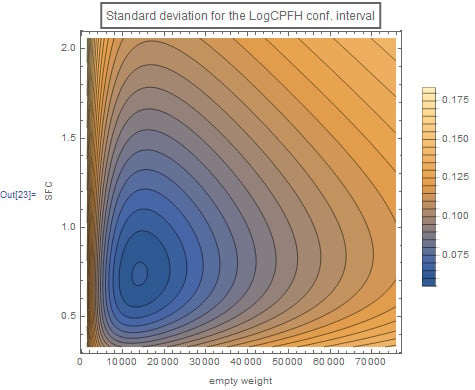
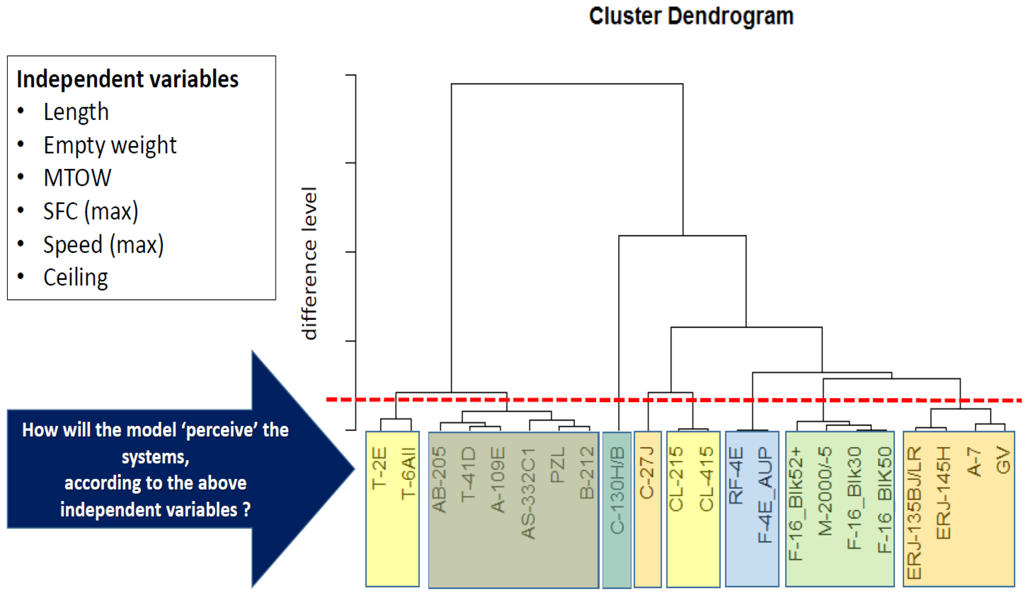
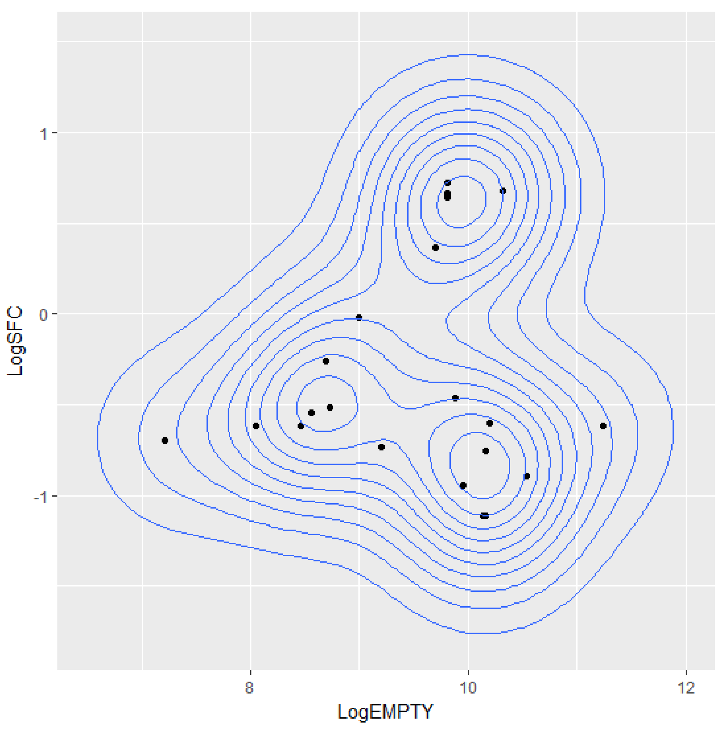
- The aircraft sample is comprised by a well-balanced mix of fixed and rotary wing aircraft types which perform a plethora of different missions, from typical military nature (air defence and superiority, interception, aerial support to land and sea military operations) to public service nature ones (fire-fighting, search and rescue, air transportation of VIPs and equipment, medical evacuations). Despite the fact that a high degree of diversification exists in the training sample, a statistically significant CER was obtained consisting of the empty weight and the SFC. This CER seems realistic since both the SFC and aircraft weight are expected to be positively related with the energy consumed during a flying hour.
- The aircraft sample has reached maturity in terms of maximum fleet numbers and this is considered a very crucial condition for sound cost estimates, especially in case of comparing CPFH of different aircraft types [1]. Most of the aircraft sample types are legacy ones with stabilized CPFH, with the newest type (F-16C/D Block 52+Adv) approaching already ten years of operational life within the HAF.
- There is no significant variation of the utilization rates of the sample, mainly because of the fact that the engagement of HAF aircraft to war conflicts outside its national borders, conditions which require unpredictable aircraft utilization rate ‘spikes’ for prolonged periods of time, is minimal. The analysis of fleet data during the Operation Desert Storm and the operations at Kosovo [4,5] suggests that the CPFH proportional model fails when a fleet of aircraft significantly changes its flight behaviour from one time interval to the next (wartime surge for example). Furthermore, Boito et al. [1] suggest that the cost of fleets should be compared using stable annual flying hours required for crew proficiency, excluding flying hours for contingency operations. Of course, as many other NATO Air Forces, HAF actively conducts and participates in large scale military exercises within the country and abroad and there might be occasions in which the utilization rates would fluctuate but overall, they are considered as stable on an annual basis.
5. Conclusions
Author Contributions
Funding
Conflicts of Interest
Acronyms
| AIC | Akaike Information Criterion |
| ANOVA | Analysis of Variance |
| CER | Cost Estimating Relationship |
| CI | Confidence Interval |
| COTS | Commercial-Off-The-Shelf |
| CPFH | Cost Per Flight Hour |
| DoD | Department of Defense (US) |
| FY | Fiscal Year |
| GAO | Government Accountability Office (US) |
| HAF | Hellenic Air Force |
| ICEAA | International Cost Estimating and Analysis Association (merger of SCEA and ISPA) |
| ISPA | International Society of Parametric Analysts |
| JSF | Joint Strike Fighter |
| LCC | Life Cycle Cost |
| MTOW | Maximum Take-Off Weight |
| MUPE | Minimum Unbiased Percentage Error |
| NATO | North Atlantic Treaty Organization |
| OGGG | Official Governmental Gazette of Greece |
| OLS | Ordinary Least Squares |
| O&S | Operating and Support |
| OSD | Office of the Secretary of Defense (US) |
| PI | Prediction Interval |
| RMS | Reliability-Maintainability-Supportability |
| ROM | Rough Order of Magnitude |
| SAR | Selected Acquisition Report |
| SCEA | Society of Cost Estimating and Analysis |
| SFC | Specific Fuel Consumption |
| USAF | United States Air Force |
| US DoD | United States Department of Defence |
| ZMPE | Zero Bias Minimum Percent Error |
References
- Boito, M.; Keating, E.G.; Wallace, J.; DeBlois, B.; Blum, I. Metrics to Compare Aircraft Operating and Support Costs in the Department of Defense; Report number RR-1178-OSD; RAND Corporation: Santa Monica, CA, USA, 2015. [Google Scholar]
- Hildebrandt, G.G.; Sze, M.B. An Estimation of USAF Aircraft Operating and Support Cost Relations; Report number N-2499-AF; RAND Corporation: Santa Monica, CA, USA, 1990. [Google Scholar]
- Sherbrooke, C.C. Using Sorties vs Flying Hours to Predict Aircraft Spares Demand; Report number LMI-AF501LN1; Logistics Management Institute: McLean, VA, USA, 1997. [Google Scholar]
- Wallace, J.M.; Houser, S.A.; Lee, D.A. A Physics-Based Alternative to Cost-Per-Flight-Hour Models of Aircraft Consumption Costs; Report number LMI-AF909T1; Logistics Management Institute: McLean, VA, USA, 2000. [Google Scholar]
- Lee, D.A. The Cost Analyst’s Companion; Logistics Management Institute: McLean, VA, USA, 1997; ISBN 9780985396504. [Google Scholar]
- Laubacher, M.E. Analysis and Forecasting of Air Force Operating and Support Cost for Rotary Aircraft; Biblioscholar, 2012; ISBN 9781288286126. Available online: https://www.bookdepository.com/Analysis-Forecasting-Air-Force-Operating-Support-Cost-for-Rotary-Aircraft-Matthew-E-Laubacher/9781288286126 (accessed on 2 October 2018).
- Hawkins, J.C. Analysis and Forecasting of Army Operating and Support Cost for Rotary Aircraft. Master’s Thesis, Air Force Institute of Technology, Wright-Patterson Air Force Base, Dayton, OH, USA, 2004. [Google Scholar]
- Armstrong, P.D. Developing an Aggregate Marginal Cost Per Flying Hour Model for the U.S. Air Force’s F-15 Fighter Aircraft; Biblioscholar, 2012; ISBN 9781288335183. Available online: https://www.bookdepository.com/Developing-an-Aggregate-Marginal-Cost-Per-Flying-Hour-Model-for-the-US-Air-Forces-F-15-Fighter-Aircraft-Patrick-D-Armstrong/9781288335183 (accessed on 2 October 2018).
- Hess, T.J. Cost Forecasting Models for the Air Force Flying Hour Program. Master’s Thesis, Air Force Institute of Technology, Wright-Patterson Air Force Base, Dayton, OH, USA, 2009. [Google Scholar]
- Hawkes, E.M.; White, E.D. Predicting the cost per flying hour for the F-16 using programmatic and operational data. J. Cost Anal. Manag. 2007, 9, 15–27. [Google Scholar] [CrossRef]
- Hawkes, E.M.; White, E.D. Empirical evidence relating aircraft age and operating and support cost growth. J. Cost Anal. Parametr. 2008, 1, 31–43. [Google Scholar]
- Unger, E.J. An Examination of the Relationship between Usage and Operating-and-Support Costs of U.S. Air Force Aircraft; Document number TR-594-AF; RAND Corporation: Santa Monica, CA, USA, 2009. [Google Scholar]
- Smirnoff, J.P.; Hicks, M.J. The impact of economic factors and acquisition reforms on the cost of defense weapon systems. Rev. Financ. Econ. 2008, 17, 3–13. [Google Scholar] [CrossRef]
- Christensen, D.S.; Searle, D.A.; Vickery, C. The Impact of the Packard Commission’s Recommendations on Reducing Cost Overruns on Defense Acquisition Contracts; Department of the Air Force: Washington, DC, USA, 1999. [Google Scholar]
- McNutt, R. Reducing DoD Product Development Time: The Role of the Schedule Development Process. Ph.D. Thesis, Massachusetts Institute of Technology, Cambridge, MA, USA, 1998. [Google Scholar]
- Office of the Secretary of Defense, Cost Assessment and Program Evaluation (OSD CAPE). Operating and Support Cost-Estimating Guide; Office of the Secretary of Defense: Washington, DC, USA, 2014. [Google Scholar]
- Bozoudis, M. Case study: A parametric model for the Cost Per Flying Hour. In Proceedings of the ICEAA International Training Symposium, Bristol, UK, 17–20 October 2016. [Google Scholar]
- International Society of Parametric Analysts. Parametric Estimating Handbook, 4th ed.; International Society of Parametric Analysts: Vienna, VA, USA, 2008. [Google Scholar]
- Defense Acquisition University. Integrated Defense Acquisition, Technology, and Logistics Life Cycle Management Framework Chart, v5.2; Defense Acquisition University: Fort Belvoir, VA, USA, 2008. [Google Scholar]
- Office of the Secretary of the Air Force. Technical Order 00-20-2: Maintenance Data Documentation, (Change 2-2007), Appendix L: “Air Force Standard Algorithms; Office of the Secretary of Defense: Washington, DC, USA, 2016. [Google Scholar]
- Office of the Secretary of the Air Force. United States Air Force Cost Risk and Uncertainty Analysis Handbook (2007), par. 2.2.2.1 and 2.2.2.3.; Office of the Secretary of Defense: Washington, DC, USA, 2007. [Google Scholar]
- United States Government Accountability Office. Cost Estimating and Assessment Guide: Best Practices for Developing and Managing Capital Program Costs; GAO-09-3SP; United States Government Accountability Office: Washington, DC, USA, 2009. [Google Scholar]
- Hellenic Air Force (HAF) Official Web Site. Available online: www.haf.gr (accessed on 19 August 2018).
- Bryant, M.T. Forecasting the KC-135 Cost per Flying Hour: A Panel Data Analysis. Master’s Thesis, Air Force Institute of Technology, Wright-Patterson Air Force Base, Dayton, OH, USA, 2007. [Google Scholar]
- United States Government Accountability Office. F-35 Sustainment: Need for Affordable Strategy, Greater Attention to Risks, and Improved Cost Estimates; Report GAO-14-778; United States Government Accountability Office: Washington, DC, USA, 2014. [Google Scholar]
- Birkler, J.; Graser, J.C.; Arena, M.V.; Cook, C.R.; Lee, G.; Lorell, M.; Smith, G.; Timson, F.; Younossi, O. Assessing Competitive Strategies for the Joint Strike Fighter: Opportunities and Options; Report number MR-1362.0-OSD/JSF; RAND Corporation: Santa Monica, CA, USA, 2001. [Google Scholar]
- United States Government Accountability Office. Fighter Aircraft: Better Cost Estimates Needed for Extending the Service Life of Selected F-16s and F/A-18s; Report GAO-13-51; United States Government Accountability Office: Washington, DC, USA, 2012. [Google Scholar]
- United States Government Accountability Office. Improvements Needed to Enhance Oversight of Estimated Long-Term Costs for Operating and Supporting Major Weapon Systems; GAO-12-340; United States Government Accountability Office: Washington, DC, USA, 2012. [Google Scholar]
- United States Government Accountability Office. Defense Acquisitions: A Knowledge-Based Funding Approach Could Improve Major Weapon System Program Outcomes; Report GAO-08-619; United States Government Accountability Office: Washington, DC, USA, 2008. [Google Scholar]
- Abell, J.B.; Kirkwood, T.F.; Petruschell, R.L.; Smith, G.K. The Cost and Performance Implications of Reliability Improvements in the F-16A/B Aircraft; Report number N-3062-ACQ; RAND Corporation: Santa Monica, CA, USA, 1988. [Google Scholar]
- Bozoudis, M.; Lappas, I.; Kottas, A. Use of cost-adjusted importance measures for aircraft maintenance system maintenance optimization. Aerospace 2018, 5, 68. [Google Scholar] [CrossRef]
- F-35 Lightning II Program Office. F-35 Lightning II Joint Strike Fighter (JSF) Program Selected Acquisition Report 2016; RCS: DD-A&T (Q&A) 823-198; F-35 Lightning II Program Office: Arlington, VA, USA, 2017. [Google Scholar]


| Aircraft/Helicopter Type | CPFH (FY 2012, €) | CPFH (FY 2013, €) | CPFH (FY 2018, €) |
|---|---|---|---|
| Helicopters | |||
| B-212 | 10,089.9 | 3133.63 | 2297.00 |
| AS-322C1 | 3142.43 | 3352.00 | 3583.64 |
| AB-205 | 3790.32 | 3505.24 | 2479.77 |
| A-109E | 2800.21 | 2678.12 | 1788.13 |
| Transport aircraft | |||
| C-130H/B | 7370.88 | 7312.81 | 5887.34 |
| C-27J | 3174.90 | 4088.80 | 9114.23 |
| Airborne Early Warning & Control aircraft | |||
| EMB-145H | 9226.77 | 7570.15 | 4292.80 |
| VIP aircraft | |||
| EMB-135 | 3545.58 | 4904.08 | 3162.17 |
| Gulfstream V | 3192.92 | 5537.09 | 3514.70 |
| Training aircraft | |||
| T-41 | 3415.60 | 1449.12 | 1314.07 |
| T-6A | 1794.40 | 1839.08 | 2127.99 |
| T-2 | 4206.68 | 4240.92 | 5154.07 |
| Fire-fighting aircraft | |||
| CL-215 | 9807.82 | 8858.95 | 7117.25 |
| CL-415 | 9508.46 | 6690.70 | 10,696.98 |
| PZL | 2492.69 | 1712.34 | 2884.25 |
| Fighter aircraft | |||
| F-16C/D | Classified | Classified | Classified |
| F/RF-4E | Classified | Classified | Classified |
| M2000/-5 | Classified | Classified | Classified |
| A-7H | Classified | Classified | Classified |
| Constraints and Requirements | Model Performance |
|---|---|
| Use the sample of 22 aircraft types operated by the HAF. | Satisfactory. |
| Use the appropriate cost information. | Satisfactory: Official FY 2013 CPFH data was used, excluding the ‘indirect support’ cost category. |
| Use cost drivers (independent variables) that are easily accessible and quantifiable. | Satisfactory: The cost drivers are aircraft physical and performance characteristics. |
| The model must be as less complex as possible and include no more than two cost drivers. | Satisfactory: The selected model includes two independent variables. |
| The model should be statistically significant at the 5% level. | Satisfactory: |
| The model should capture at least 75% of the CPFH variance. | Satisfactory: |
| The model’s confidence and prediction intervals must be valid. | Satisfactory: The residuals do pass all the appropriate tests. |
| The model’s mathematical expression should make sense. | Satisfactory: The model suggests that the aircraft empty weight and the engine SFC correlate positively with the CPFH. |
| Variables | Variable Trans-Formation | Transformed Variable Notation | Assessment Tests * for Linearity among Variable and LogCPFH (‘Ø’ Indicates p-Value < 0.05) | ||||
|---|---|---|---|---|---|---|---|
| Test 1 a | Test 2 b | Test 3 c | Test 4 d | Test 5 e | |||
| Dependent | |||||||
| CPFH, €/h | Log | LogCPFH | |||||
| Independent | |||||||
| Length (longitudinal axis), ft | Log | LogLENGTH | Ø | Ø | |||
| Empty weight, lb | Log | LogEMPTY | |||||
| MTOW, lb | Log | LogMTOW | |||||
| Max SFC, lb/(lbf∙h) or lb/(hp∙h) | Log | LogSFC | |||||
| Max speed, km/h | Log | LogSPEED | |||||
| Ceiling, ft | ×10−4 | AdjCEIL | |||||
| Model Selection | |||||
|---|---|---|---|---|---|
| Start: AIC = −56.02 | |||||
| LogCPFH ~ LogEMPTY * LogSFC | |||||
| Df | Sum of Sq | RSS | AIC | ||
| LogEMPTY:LogSFC | 1 | 0.040019 | 1.2384 | −57.298 | |
| <none> | 1.1984 | −56.021 | |||
| Step: AIC = −57.3 | |||||
| LogCPFH ~ LogEMPTY + LogSFC | |||||
| Df | Sum of Sq | RSS | AIC | ||
| <none> | 1.2384 | −57.298 | |||
| −LogSFC | 1 | 1.5185 | 2.7569 | −41.692 | |
| −LogEMPTY | 1 | 4.1550 | 5.3934 | −26.929 | |
| Residuals | |||||
| Min | 1Q | Median | 3Q | Max | |
| −0.42125 | −0.08515 | −0.02154 | 0.09199 | 0.50650 | |
| Coefficients | |||||
| Estimate | Std. Error | t value | Pr(>|t|) | ||
| (Intercept) | −4.95006 | 0.57456 | −8.615 | 5.48 × 10⁻⁸ | |
| LogEMPTY | 0.47510 | 0.05951 | 7.984 | 1.73 × 10⁻⁷ | |
| LogSFC | 0.42793 | 0.08866 | 4.827 | 0.000117 | |
| Residual standard error: 0.2553 on 19 degrees of freedom Multiple R-squared: 0.8385, Adjusted R-squared: 0.8215 F-statistic: 49.31 on 2 and 19 DF, p-value: 3.009 × 10⁻⁸ | |||||
| Correlation of Coefficients | |||||
| (Intercept) | LogEMPTY | ||||
| LogEMPTY | −0.99 | ||||
| LogSFC | 0.17 | −0.13 | |||
| Analysis of Variance Table | |||||
| Response: LogCPFH | |||||
| Df | Sum Sq | Mean Sq | F value | Pr(>F) | |
| LogEMPTY | 1 | 4.9099 | 4.9099 | 75.327 | 4.895 × 10⁻⁸ |
| LogSFC | 1 | 1.5185 | 1.5185 | 23.296 | 0.0001172 |
| Residuals | 19 | 1.2384 | 0.0652 | ||
| --- | |||||
| bcnPower Transformation to Normality | |||||
| Estimated power, lambda | |||||
| Est Power | Rounded Pwr | Wald Lwr Bnd | Wald Upr Bnd | ||
| Y1 | −1.2543 | 1 | −5.4661 | 2.9574 | |
| Location gamma was fixed at its lower bound | |||||
| Est gamma | Std Err. | Wald Lower Bound | Wald Upper Bound | ||
| Y1 | 0.1 | NA | NA | NA | |
| Likelihood ratio tests about transformation parameters | |||||
| LRT | Df | pval | |||
| LR test, lambda = (0) | 0.3258308 | 1 | 0.5681244 | ||
| LR test, lambda = (1) | 1.0123004 | 1 | 0.3143524 | ||
| Assessment of the Linear Model Assumptions | |||||
| Value | p-value | Decision | |||
| Global Stat | 0.776499 | 0.9416 | Assumptions acceptable. | ||
| Skewness | 0.593439 | 0.4411 | Assumptions acceptable. | ||
| Kurtosis | 0.001988 | 0.9644 | Assumptions acceptable. | ||
| Link Function | 0.177909 | 0.6732 | Assumptions acceptable. | ||
| Heteroscedasticity | 0.003163 | 0.9552 | Assumptions acceptable. | ||
| Test | Null Hypothesis | p-Value | Reject the Null Hypothesis at the 5% Significance Level? |
|---|---|---|---|
| Shapiro-Wilk normality test | Normality | 0.161 | NO |
| Breusch-Pagan test for heteroscedasticity | Constant variance | 0.332 | NO |
| Durbin-Watson test for autocorrelation | Randomness | 0.302 | NO |
| Two-sided t-test with Bonferroni adjustment | No outliers | 0.714 | NO |
| Aircraft | CPFH Lower Bound | CPFH Expected | CPFH Upper Bound |
|---|---|---|---|
| T-41D | 0.11901211 | 0.16420763 | 0.22162284 |
| A-109E | 0.19990530 | 0.25036102 | 0.31012026 |
| T-6A II | 0.25249018 | 0.30355962 | 0.36225471 |
| AB-205 | 0.27634370 | 0.32830309 | 0.38749658 |
| B-212 | 0.30764429 | 0.35999624 | 0.41896993 |
| PZL | 0.33723845 | 0.39536636 | 0.46093791 |
| AS-332C1 | 0.35547705 | 0.41073767 | 0.47240366 |
| T-2E | 0.43697559 | 0.50679004 | 0.58491362 |
| GV | 0.44894272 | 0.53734944 | 0.63862291 |
| EMB-135BJ/LR | 0.44230344 | 0.54767037 | 0.67142878 |
| EMB-145H | 0.44643551 | 0.55351426 | 0.67940476 |
| A-7 | 0.55941742 | 0.63567511 | 0.71971577 |
| CL-415 | 0.54352594 | 0.64380037 | 0.75778338 |
| CL-215 | 0.59726742 | 0.69851969 | 0.81253214 |
| C-27J | 0.58484956 | 0.72391072 | 0.88720093 |
| M-2000/-5 | 0.70287959 | 0.83413491 | 0.98354446 |
| F-16 Block 50 | 0.80040814 | 0.99097233 | 1.21478042 |
| F-16 Block 52+ | 0.80500314 | 1.00000000 | 1.22957677 |
| F-16 Block 30 | 0.81828962 | 1.02648845 | 1.27337004 |
| C-130H/B | 0.87955200 | 1.14080188 | 1.45822407 |
| RF-4E | 1.01709601 | 1.28261782 | 1.59868855 |
| F-4E AUP | 1.01709601 | 1.28261782 | 1.59868855 |
| Aircraft | CPFH Lower Bound | CPFH Expected | CPFH Upper Bound |
|---|---|---|---|
| P2002JF | 0.06753461 | 0.10155222 | 0.14747995 |
| RACER | 0.27574280 | 0.32714039 | 0.38563437 |
| AW189 | 0.33099377 | 0.38469385 | 0.44488060 |
| HH-60W | 0.43900130 | 0.50855135 | 0.58631201 |
| M-346 | 0.45194200 | 0.51116159 | 0.57619763 |
| A-10A | 0.46891536 | 0.57069196 | 0.68872595 |
| AV-8B | 0.53926887 | 0.60547233 | 0.67777883 |
| T-X | 0.48855572 | 0.61262218 | 0.75969810 |
| T-100 | 0.56187968 | 0.63154563 | 0.70769602 |
| T-50 | 0.69523642 | 0.84927503 | 1.02840736 |
| JAS-39 | 0.71724836 | 0.87968786 | 1.06914862 |
| F/A-18C/D | 0.86861590 | 1.06510753 | 1.29424863 |
| Eurofighter | 0.87437845 | 1.06688394 | 1.29056054 |
| Rafale C | 0.88019674 | 1.10117609 | 1.36269648 |
| AC-130U | 0.87930885 | 1.14038891 | 1.45758505 |
| F-35A | 0.99567786 | 1.25154867 | 1.55541068 |
| J-31 | 1.03666736 | 1.31599161 | 1.65010582 |
| F-15E | 1.05604359 | 1.34694738 | 1.69611550 |
| Su-27SK | 1.09117401 | 1.38460952 | 1.73549656 |
| Su-57 | 1.14592428 | 1.46794227 | 1.85568007 |
| F-22A | 1.24714749 | 1.64265811 | 2.12859570 |
© 2018 by the authors. Licensee MDPI, Basel, Switzerland. This article is an open access article distributed under the terms and conditions of the Creative Commons Attribution (CC BY) license (http://creativecommons.org/licenses/by/4.0/).
Share and Cite
Lappas, I.; Bozoudis, M. The Development of an Ordinary Least Squares Parametric Model to Estimate the Cost Per Flying Hour of ‘Unknown’ Aircraft Types and a Comparative Application †. Aerospace 2018, 5, 104. https://doi.org/10.3390/aerospace5040104
Lappas I, Bozoudis M. The Development of an Ordinary Least Squares Parametric Model to Estimate the Cost Per Flying Hour of ‘Unknown’ Aircraft Types and a Comparative Application †. Aerospace. 2018; 5(4):104. https://doi.org/10.3390/aerospace5040104
Chicago/Turabian StyleLappas, Ilias, and Michail Bozoudis. 2018. "The Development of an Ordinary Least Squares Parametric Model to Estimate the Cost Per Flying Hour of ‘Unknown’ Aircraft Types and a Comparative Application †" Aerospace 5, no. 4: 104. https://doi.org/10.3390/aerospace5040104
APA StyleLappas, I., & Bozoudis, M. (2018). The Development of an Ordinary Least Squares Parametric Model to Estimate the Cost Per Flying Hour of ‘Unknown’ Aircraft Types and a Comparative Application †. Aerospace, 5(4), 104. https://doi.org/10.3390/aerospace5040104