1. Introduction
The accurate prediction of the flow development inside various stations in an aero engine (e.g., compressor and turbine stages, intakes, nozzles, combustors, heat exchangers) is of great interest to aero engine designers since the understanding of the flow underlying physics and its development are critical in order to enhance their operational performance and provide efficient aero engines architectures. Nowadays, many design methodologies of aero engine turbomachinery components exist that are able to provide good and rapid solutions regarding their components’ geometrical design and characteristics with certain limitations, since the computation of the accurate flow field especially inside compressors and turbines, requires the use of Computational Fluid Dynamics (CFD), which is more computationally demanding. However, with increasing available CPU power, CFD methodologies and algorithms become more and more attractive for engineers and turbomachinery designers. These methodologies include turbulence modelling and Reynolds Averaged Navier Stokes (RANS) equation solutions, Detached and Large Eddy Simulation (DES, LES) models and hybrid approaches combining the above (hybrid RANS/LES). The use of LES based methodologies require increased computational resources and are time consuming while on the other hand, turbulence modelling using RANS approaches are more time efficient and require less computational power. Under this perspective, especially from an engineering point of view where time efficient computations are of great importance, RANS and turbulence modelling methodologies have become a basic engineering tool for the last 20 years. However, the use of turbulence modelling requires good knowledge of the physics and the mathematical relations that are the building blocks of these methodologies. Additionally, understanding the limits or the advantages of turbulence models for the calculation of complex flow fields (such as transitional and unsteady flows that are met inside turbomachinery) is a key aspect to further improving the computational methodologies, algorithms, and techniques.
In the literature there are numerous studies regarding CFD computations and turbulence modelling of the flow around compressor and turbine blades in turbomachinery, which is also the main topic of the current work. For instance, Biesenger et al. [
1] adopted linear eddy-viscosity models with appropriate refinements in order to study the flow in subsonic and transonic compressors. Additionally, as presented in [
2], the authors utilized zero and two equation turbulence models and provided a comparison to experimental data for axial turbomachinery flows (compressors and turbine blades), and it was proved that the adopted models provided results closer to the experiments, concluding that for the accurate modelling of such kind of flows, extension to transitional and higher order turbulence models are necessary. In the same direction, Dawes [
3] presented turbulence modelling predictions for a compressor transonic cascade blade and a linear low pressure turbine cascade by adopting a single mixing length model and an one equation turbulence model. Zhang et al. [
4] utilized a Reynolds stress model and a linear eddy viscosity model for the flow modelling of a typical high-speed compressor cascade providing useful data for the turbomachinery flow modelling and the adopted turbulence models’ performance. Suthakar and Dhurandhar [
5] modelled the flow in an axial flow compressor with the realizable k-ε turbulence model focusing on the prediction of the secondary flow formation. Kumar et al. [
6] presented a performance assessment of the standard k-ε model, the realizable k-ε model, and the k-klaminar-ω turbulence model for the flow modelling of a centrifugal compressor of a micro gas turbine. Gourdain [
7] compared Large Eddy Simulation (LES) computations with Unsteady Reynolds Averaged Navier Stokes Equations (URANS) computations by adopting the linear k-ω and k-ε models and available experimental data for the flow of an axial compressor stage, stating that the better understanding of the unsteady flow that is met in turbomachinery components is of great importance for efficient aero engine components design. Andrei [
8] utilized 4 turbulence models in order to model a two-dimensional (2D) high loaded rotating cascade of an axial compressor and predict the lift and drag coefficients. Ning et al. [
9] implemented RANS equations with the use of the Spalart-Almaras one equation turbulence model focusing on the three-dimensional (3D) aerodynamic redesign of a 5-stage compressor with multi stage CFD methods. Menter and Langtry [
10] presented a detailed study regarding the turbulence modelling approaches for the accurate prediction of the flow development in turbomachinery. Vlahostergios et al. [
11] evaluated a cubic non-linear k-ε model performance comparing the results with available experimental data for the flow prediction of the anisotropic wake of a low pressure turbine blade.
In the current work, a detailed performance assessment of three turbulence models regarding their accuracy in modelling a complex unsteady flow field around a Double Circular Arc (DCA) compressor blade are presented. The examined test case uses the well-known compressor blade whose flow field development was measured and presented in the work of Deutsch and Zierke [
12,
13]. The developed flow field is extremely challenging for turbulence modelling since many complex flow phenomena are present including boundary layer transition on both the pressure and the suction sides of the blade and trailing edge vortex shedding. Additionally, there are no similar computational studies in the literature that assess in such detail the turbulence models performance by providing detailed velocity and turbulence intensity distributions for all the measurement stations with unsteady computations. Additionally, a detailed investigation for the specific DCA compressor blade is limited and only few numerical data compared with the experiments are available. For the flow modelling, 4 turbulence models were utilized: the widely used eddy viscosity model of Spalart and Allmaras [
14], the linear eddy viscosity Shear Stress Transport k-ω model of Menter [
15], and two Reynolds stress models (RSM) which are the Baseline RSM (as presented in [
16]) and the non-linear RSM by Speziale et al. [
17]. The commercial CFD solver of ANSYS-CFX [
16] was used for the computations, and unsteady Reynolds averaged Navier Stokes equations were implemented in the cases where the turbulence models were able to capture the flow unsteadiness. The study presents the minor superiority (for the selected test case and turbulence models) of the RSMs by providing comparisons with available experimental data regarding velocities and turbulence intensity distributions that are available in the European Research Community on Flow, Turbulence and Combustion (ERCOFTAC) database [
18]. It is demonstrated that the models must be capable to calculate the unsteady features of the flow in order to provide more accurate computational results, especially for the turbulence intensity of the flow. As also presented and discussed in [
19,
20], it is very important to provide CFD algorithms that can resolve or model all the turbulent/small and large scales for the accurate calculations of the complex flow fields that are met in turbomachinery flows, leading to the designing of more efficient aero engine components and architectures.
4. Turbulence Modelling Results
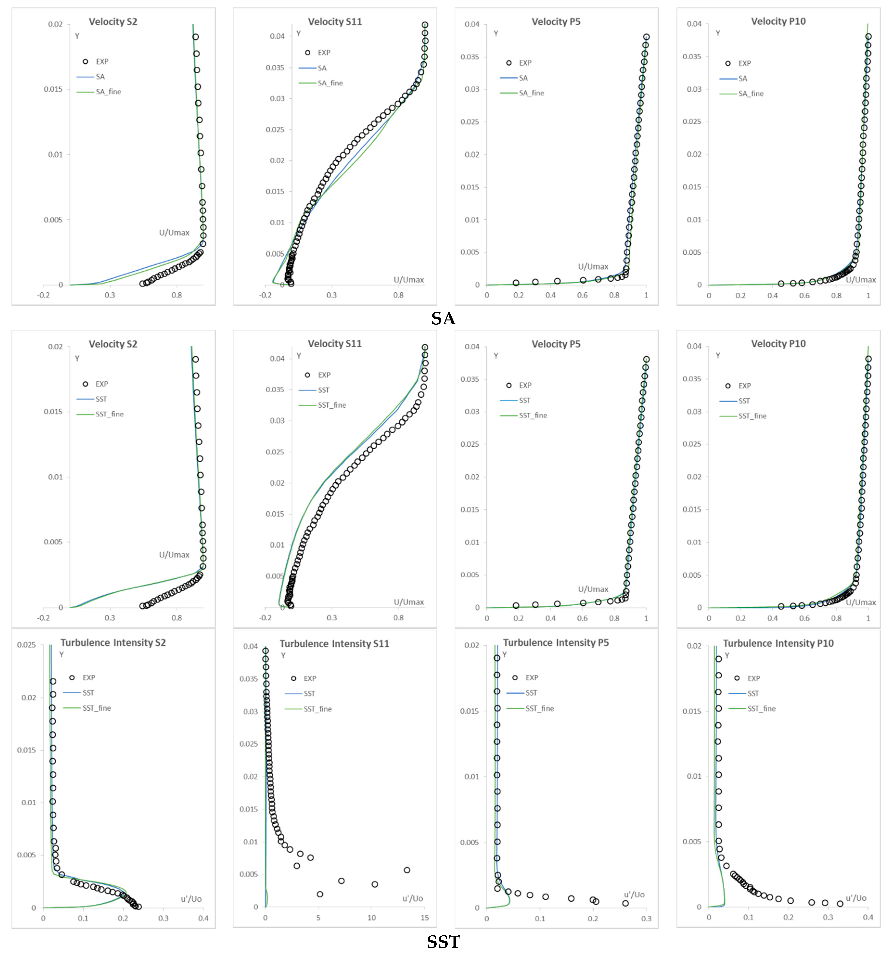
Regarding the computational results, for the SA, the SST, and BSL-RSM models, no unsteadiness was identified and steady computations were performed. However, the SSG-RSM model was able to capture flow unsteadiness due to vortex shedding from the trailing edge and hence, URANS were imposed. All the presented results concerning the SSG-RSM, derived from an averaging of the flow for an adequate sampling time which contained more than 60 periods of the time dependent velocities and turbulence intensities.
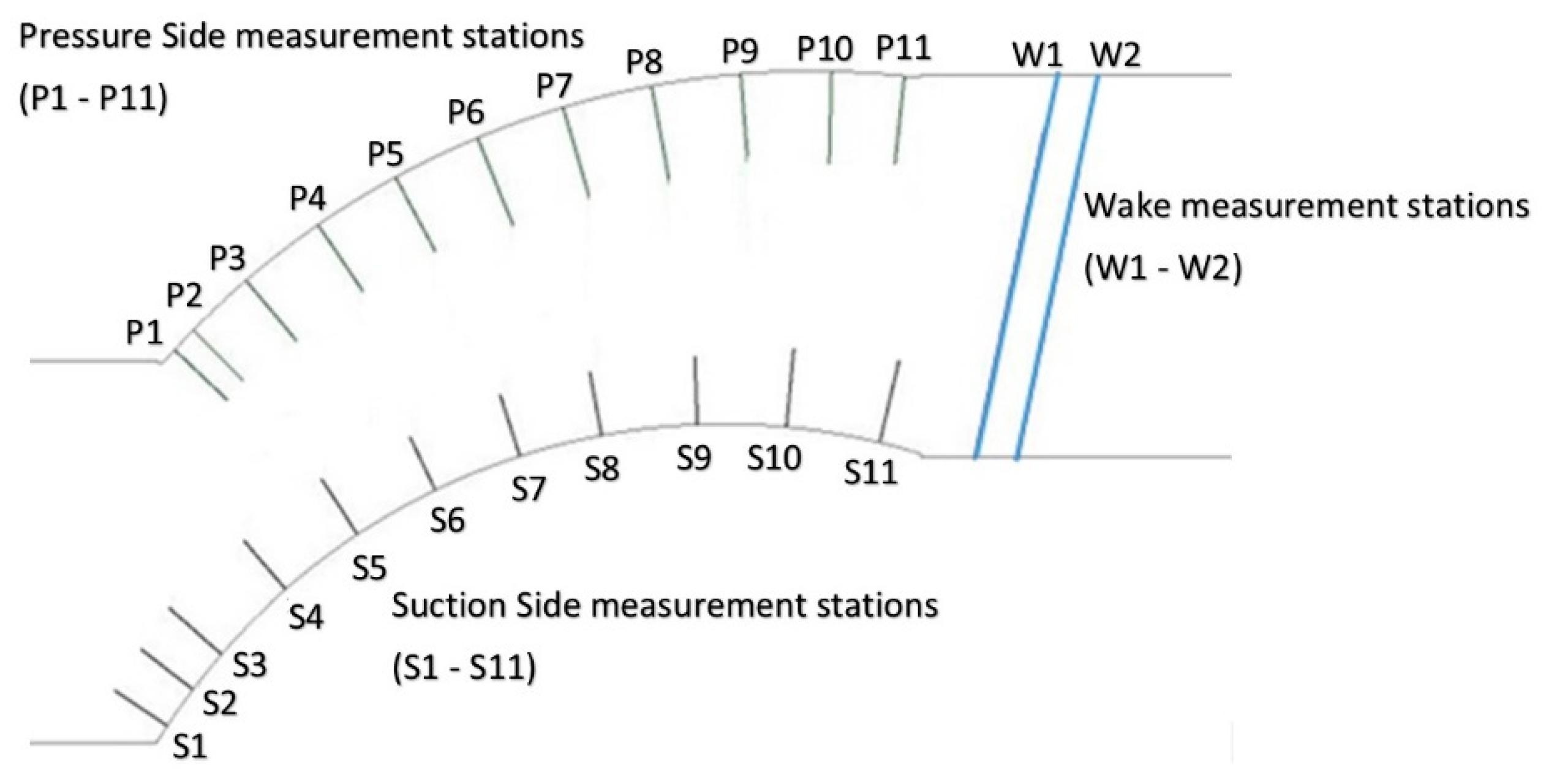
4.1. The DCA Pressure Side
The pressure side measurements include 11 measurement stations given as a percentage of the pressure side distance and coded in the present paper as shown in
Table 3.
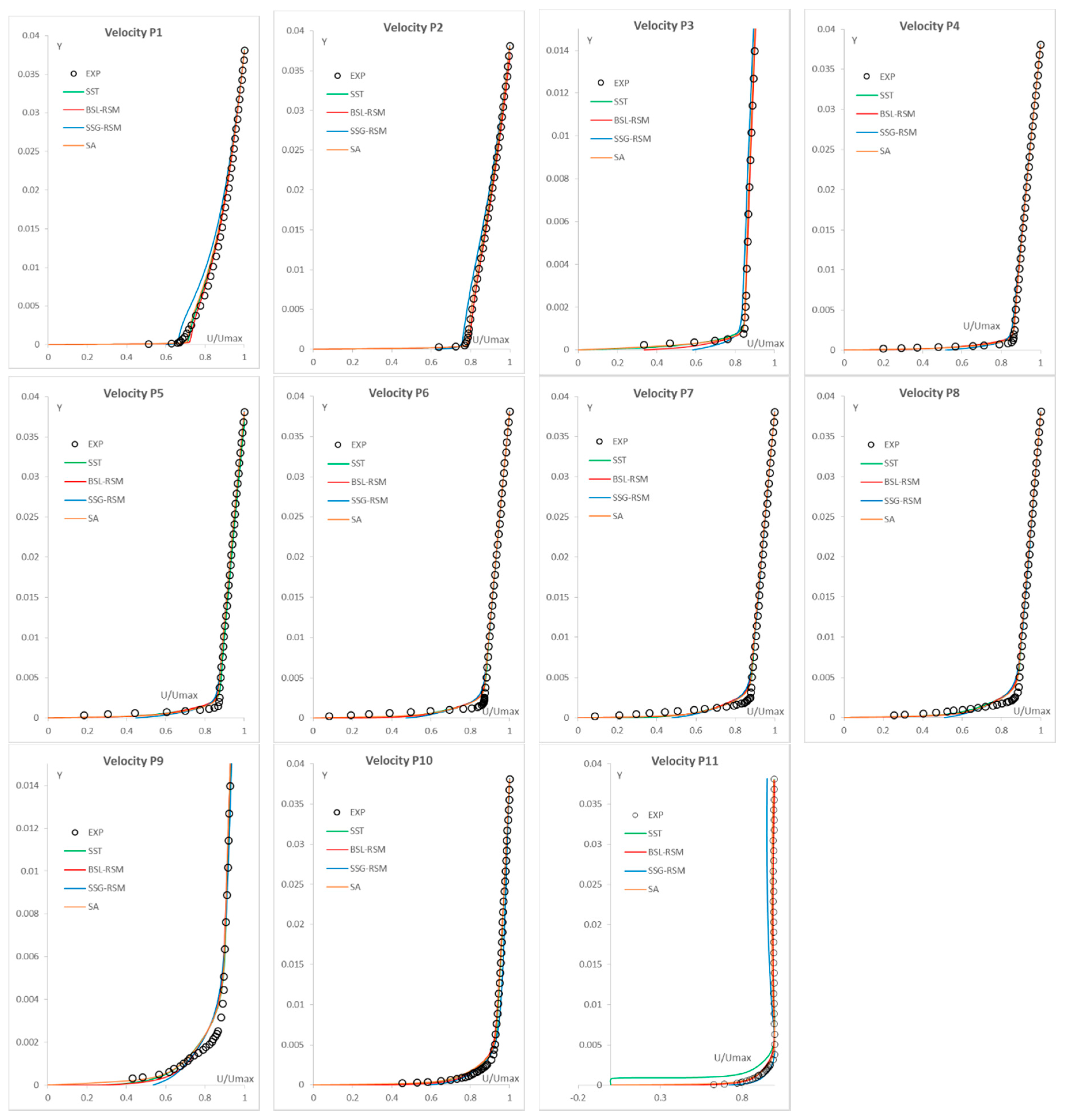
The velocity distributions comparisons are presented in
Figure 5. As it can be seen all the models are able to capture the experimental distributions shape for the majority of the measurement stations. The SST model computes a small recirculation in the last station (P11) which stays attached on the pressure side. For the rest of the stations, the SA, the BSL-RSM, and the SST provide similar results while the SSG-RSM slightly differs from the measurements for Stations P1, P2, and P11. From these observations it can be concluded that the BSL-RSM model is capable to describe in a better manner the velocity distributions on the DCA blade pressure side, although with minor superiority.
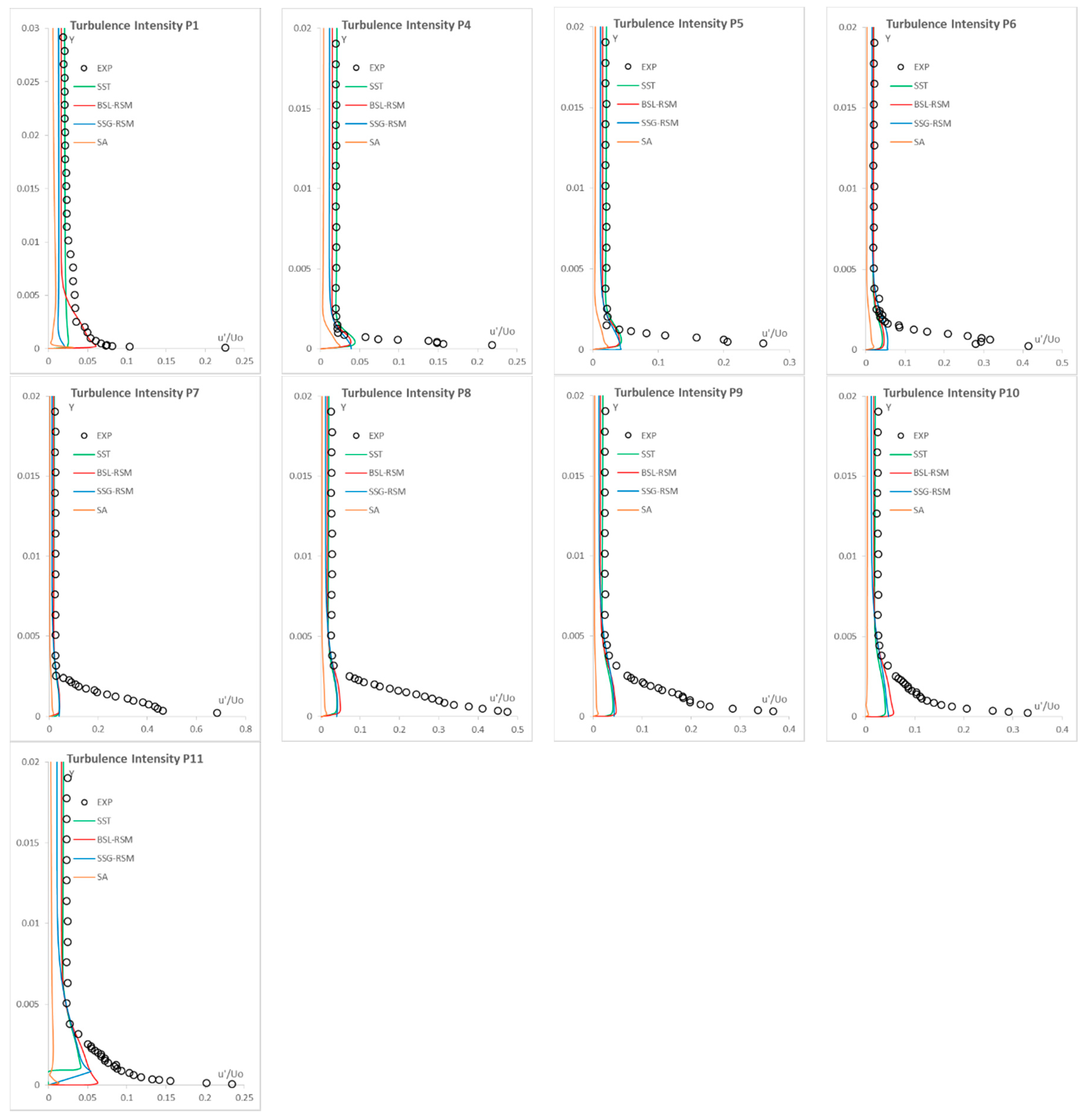
In
Figure 6 the turbulence intensity distributions on the pressure side, which is in fact the quantity
that is ploted for the turbulence models, is presented. It must be mentioned that for the SA model the turbulence intensity was caclulated from the longitudinal Reynolds stress as a function of the eddy viscosity and the mean strain rate, by neglecting the turbulence kinetic energy (
k). For the first station (P1) the SST and SSG-RSM are not able to provide an accurate turbulence intensity inside the boundary layer region. On the other hand, the BSL-RSM computes the position of the peak of the distribution, but again cannot predict the correct much larger experimental value. This is the first station of the pressure side and the computed/modelled turbulence instabilities (the free stream turbulence intensity) were not able to penetrate the boundary layer to the extent as the measurements suggest and to provide the measured turbulence intensity. As the flow approaches the trailing edge, the SST, the BSL-RSM and the SSG-RSM models provide similar results. However, in the last station (P11) the BSL-RSM provides values closer to the experimental measurements. The free stream turbulence intensity is accurately computed by all the models, which is an indication of the correct estimation of the turbulent length scale, while none of the models are able to capture the peak turbulence intensity values. Again it can be concluded that the BSL-RSM provides the most qualitative results. Finally, the SA model is not able to predict the correct turbulence intensity for all the stations. Apart from the model’s inherent characteristic in not performing well in transitional flows, this is also related to the fact that the turbulence kinetic energy is not computed by the model and the term
in the Boussinesq hypothesis (Equation (5)) is not taken into consideration to the final distributions.
4.2. DCA Suction Side
The suction side presents more interesting flow characteristics since the presence of intense adverse pressure gradients results in recirculation regions on the leading and trailing edges of the blade as reported in [
13]. Additionally, the boundary layer has transitional characteristics [
12,
13] for a large area on the suction side. This makes this flow more challenging for the turbulence models calculations. The selected measurement stations on the suction side with the corresponding distance percentage are given in
Table 4.
The velocity distributions of the turbulence models on the suction side for the 11 measurement stations of the blade are given in
Figure 7.
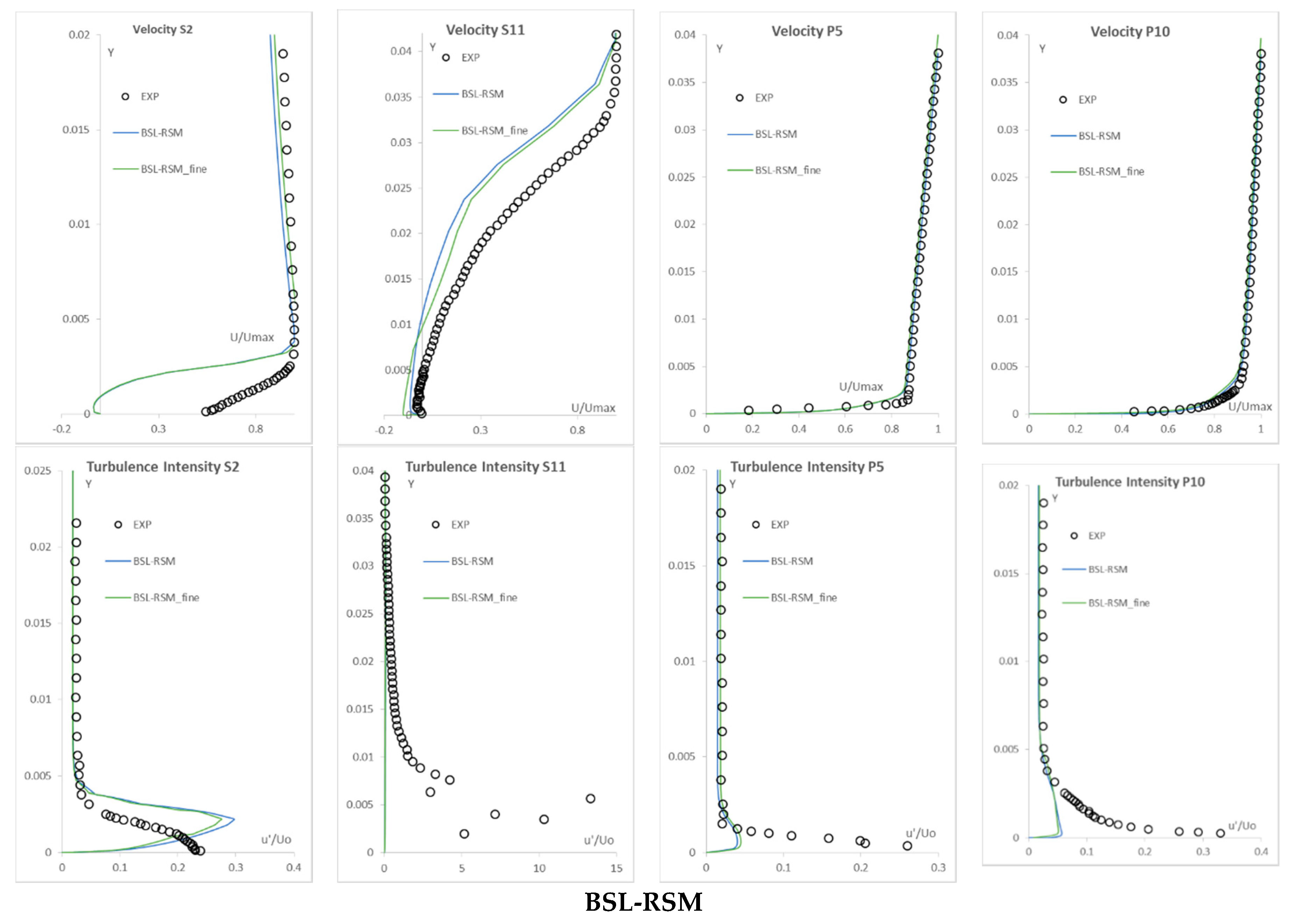
From the velocity distributions it can be concluded that the SST and the BSL-RSM present similar behaviour and they are able to predict a recirculation region towards the trailing edge (Stations S9, S10 and S11). The majority of the distributions tend to provide thicker boundary layers for all the stations. Additionally, they also compute a recirculation region in Stations S1 and S2. Although there is a recirculation region in the blade leading edge as reported in [
13], this region is smaller according to the measurements and cannot be spotted in the diagrams since the measured boundary layer is attached before Station S1. The similar behaviour of the two models is probably linked to the same modelling approach of adopting the specific turbulent dissipation rate near the wall region. On the other hand, the SSG-RSM model computes thinner boundary layers in comparison to the experiments and the SA, the SST, and BSL-RSM. Additionally, near the trailing edge, for Stations S10 and S11, it provides distributions closer to the experimental values especially near the wall region. Regarding the SA model, it provides qualitative distributions by capturing the recirculation region (closer to the SST) in the leading edge and by providing an excellent velocity distribution near the trailing edge at Station S10. As a general observation, the SA provides qualitative velocity distributions that are close to the experimental data for the DCA suction side.
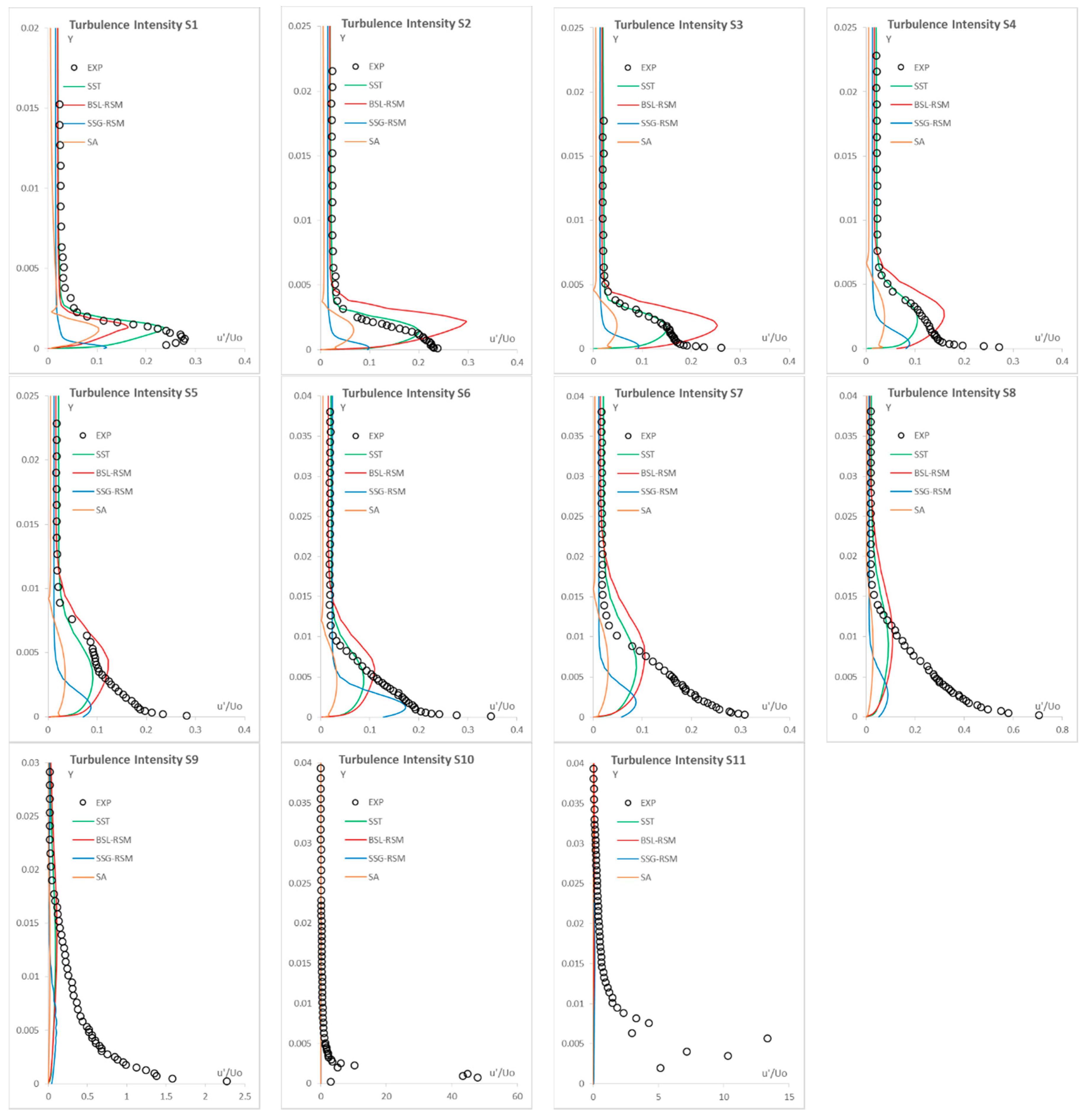
The turbulence intensity distributions (which are linked to the longitudinal Reynolds stress) are presented in
Figure 8.
As illustrated in
Figure 8, up to Station S8, all models compute smaller turbulence intensity values. From Stations S9 to S10 where the trailing edge recirculation regions begin to develop, the boundary layer relaminarizes and as a result the specific models cannot capture this behaviour by providing almost zero longitudinal Reynolds stresses values (Stations S9, S10 and S11). From the experimental values it is shown that the turbulence intensity reaches the value of 50 in Station S10, which is a strong indication of the unsteady nature of the flow due to boundary layer separation towards the trailing edge and to the contribution of large scales/eddies. The overall flow kinetic energy is the summation of the resolved large and the modelled small turbulent scales/eddies. Once again the SST and the BSL-RSM present similar behaviour by providing similar distributions along the suction side. The BSL-RSM is able to compute larger values, apart from the first station S1 where the SST as a linear eddy viscosity model computes increased turbulence generation closer to the measured one. The SSG-RSM model is not able to provide the increased values of the experiments and the BSL-RSM and SST models. However, it computes more accurately the position (on the
y-axis) of the maximum values and the experimental data curve slopes for all the stations until station S6, just before the recirculation region starts to develop. This slightly more qualitative behaviour in the results (however not quantitative) is probably linked to the cubic relation of the pressure strain correlation that the SSG-RSM adopts and is able to provide a more qualitative representation of the turbulent energy redistribution near the wall region. Despite this behaviour, the SSG-RSM cannot compute the unsteadiness near the trailing edge and provides almost zero turbulence intensity values. Finally, the SA model provides results more qualitative in relation to the pressure side turbulent intensity distributions but still cannot calculate the turbulence intensity peak values by computing smaller values in comparison to the rest of the models and the experiment. Once again, the free stream turbulence intensity is well captured by all the models and supports the selection of the inlet turbulent length scale. As an overall conclusion from the DCA suction side modelling results, the BSL-RSM is suggested as the most accurate turbulence model for the current computations.
4.3. DCA Wake Region
In the final part of the study, two measurement stations in the wake region are presented. The positions of the stations are located on the extension of the blade chord and are given in
Table 5 as a percentage of the chord length.
As was already mentioned, the SA, the SST, and the BSL-RSM models were not able to predict any flow unsteadiness and provided steady computations. On the other hand, the SSG-RSM was able to predict an unsteady flow concerning only the vortex shedding on the blade trailing edge and not any unsteady boundary layer behaviour on the suctions side (after Station S9). As a result for the SSG-RSM, URANS were implemented and in order to also compute the energy of the trailing edge eddies (large scales) of the flow, an appropriate statistical averaging was performed. The total energy of the unsteady flow was divided in two parts, as was also suggested by Davidson [
21]. The first part is the turbulence kinetic energy (the small scale energy) that the turbulence models compute and in the current study is the only part of the energy calculated by the SA, the SST and the BSL-RSM. The second part is the resolved (large scale) kinetic energy related to the flow eddies linked to the trailing edge vortex shedding and is a result of the unsteady mean flow velocity computed with URANS and the SSG-RSM. The total small and large scale kinetic energy and Reynolds stresses are given by Equations (6) and (7).
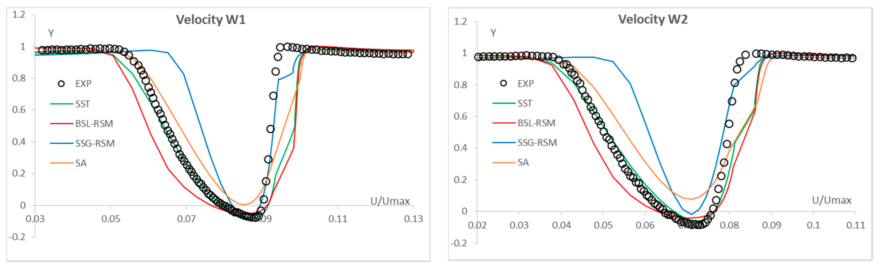
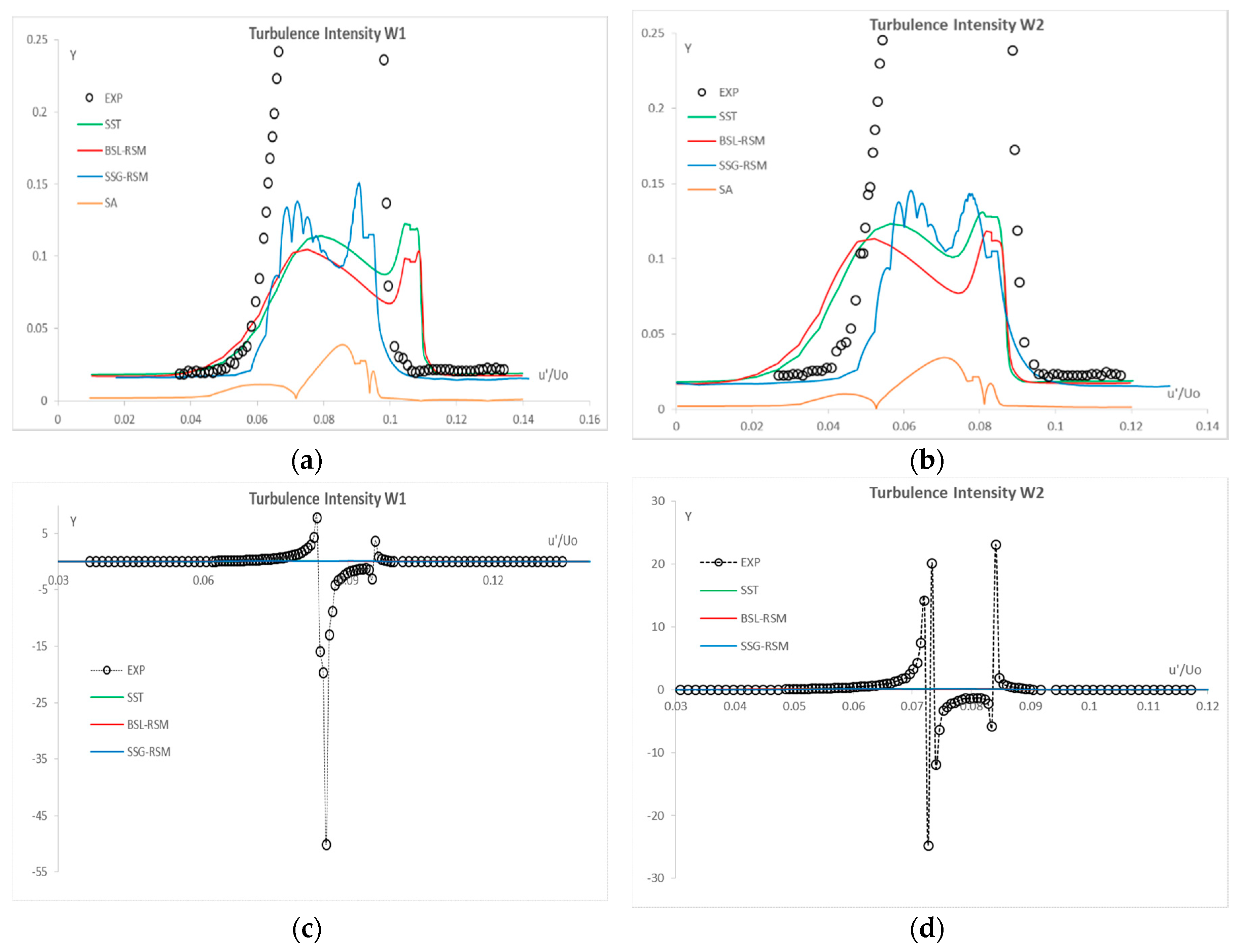
The comparisons in the wake region of the velocity and the turbulent intensity distributions for the four models are given in
Figure 9 and
Figure 10.
Once again, the SST and the BSL-RSM provide similar results regarding both the velocities and the turbulence intensities. The SSG-RSM computes narrower wake but a slightly increased turbulence intensity that is a result of the large scales contribution. Regarding the SA model, it provides smaller velocity values and also significantly smaller turbulence intensity values. This is in agreement with the fact that the SA model produces errors in calculating free shear flows and is not recommended for applications where free shear is important for the flow development. In order to give to the reader a clear view of the unsteadiness intensity in the wake region,
Figure 10a,b present a zoomed area for providing a comparable view of the results, while
Figure 10c,d show the whole measured range of the flow intensity
. As it can be seen, the quantity
takes values from −50 (W1) to 20 (W2) which are values that indicate unsteadiness and cannot be captured by the present turbulence models. Even the SSG-RSM, which is able to compute the trailing edge vortex shedding, cannot resolve the intensity of the unsteady wake.
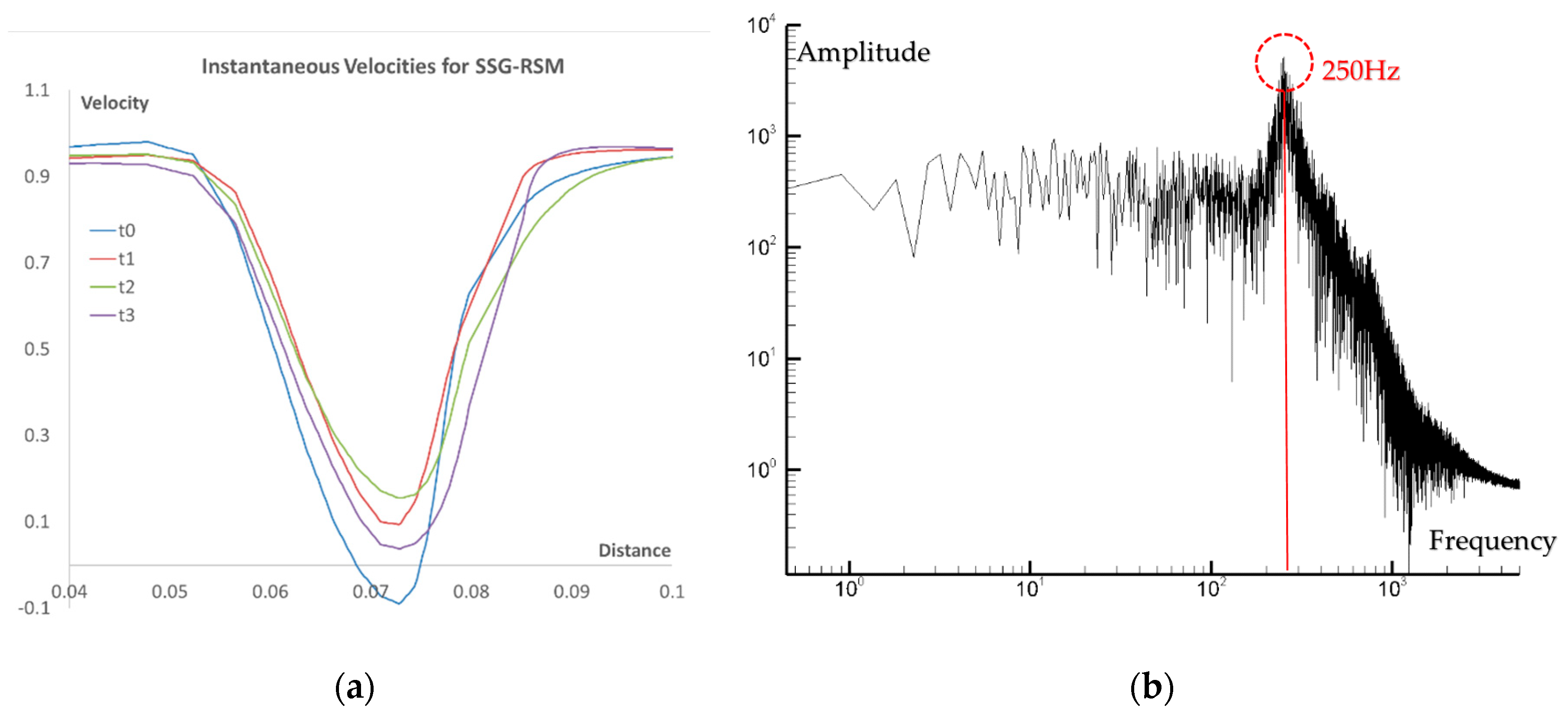
Regarding the URANS RSM-SSG computations, the flow unsteadiness was also observed by a monitor point which was monitoring the velocity fluctuations and was placed in the wake region of the blade. In
Figure 11a instantaneous velocities are presented for four indicative time instances during the computations. These observed velocity fluctuations of the mean velocity for each time step are in fact the large scales contributions to the overall calculated kinetic energy and to the large scale stresses that are given by Equations (6) and (7). The unsteady nature of the flow in the wake region is also supported by the Fourier analysis of the obtained velocity signal which is presented in
Figure 11b.
From the analysis, a dominant frequency of 250 Hz was identified, which is the frequency that characterizes the unsteady trailing edge large scales that were computed with URANS and the SSG-RSM. By observing both the measured and the computed turbulence intensity values it is evident that in order to accurately compute such complex flows and be able to capture the unsteady kinetic energy of the flow with the turbulence modelling methodology, the use of less dissipative turbulence models that will accurately model the turbulence transitional characteristics and itsgeneration due to free shear and also compute/resolve the strong unsteady nature of the flow is obligatory. As it was presented in [
11,
25], more sophisticated turbulence models (i.e., a cubic eddy viscosity model and a non-linear RSM) were able to provide qualitative results for capturing the wake development of a low pressure turbine blade.
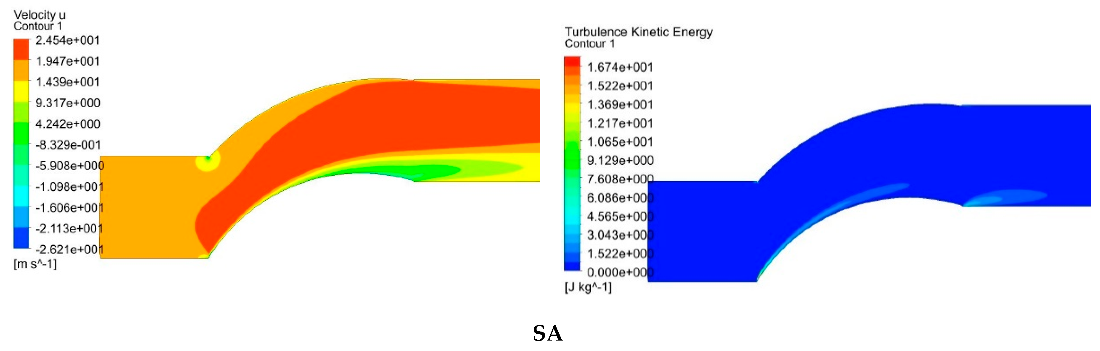
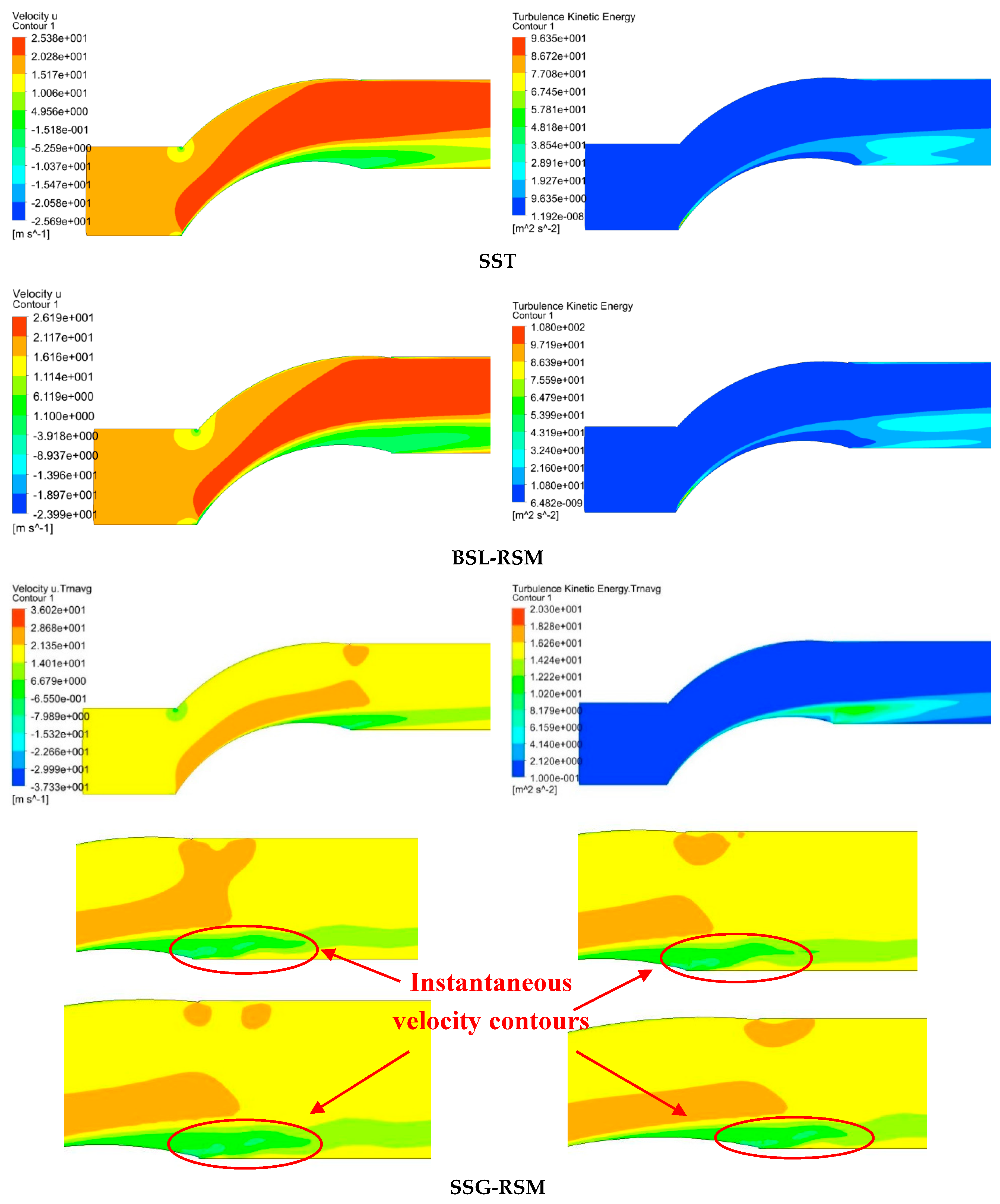
As a final step of the work, in order to provide to the reader a representation for better understanding the modelled velocity and turbulence intensity fields development, as well as the observed unsteadiness in the wake region, contour plots for all the examined models are provided in
Figure 12.
For the SSG-RSM model, apart from the time averaged velocity and turbulence kinetic energy flow field contours, additional contours regarding four indicative selected time steps for the visualization of the instantaneous velocity inside the wake region are presented. The unsteady movement of the wake can be clearly seen, which is the main contributor to the large scale kinetic energy of the flow.
5. Discussion and Conclusions
This paper presents a detailed study of four turbulence models regarding their capability of predicting the flow field over a DCA compressor blade. The examined test case was the transitional compressor blade of Zierke and Deutsch [
12,
13], which represents a very complex flow field suitable for turbulence models and CFD methodologies validation. The experimental data for the validation were taken from the ERCOFTAC classic database [
18]. The selected models were the one equation SA eddy viscosity model, the linear two equation SST eddy viscosity model and two RSM models. The RSMs were a Reynolds stress model which uses a blending function for modelling the turbulence dissipation rate and is linear regarding the pressure strain correlation term expression and a non-linear RSM which adopts the SSG [
17] non-linear relation for the mathematical description of the pressure strain correlation. From the current analysis the following conclusions can be derived:
The SA, the SST, and RSM-BSL models are too dissipative and are not able to capture the flow unsteadiness and the intensity of the produced unsteady large scales. Additionally, the SST and the RSM-BSL present the same behaviour due to the similar modelling approach they follow for the turbulence dissipation. It is expected that the omega based turbulence models would provide similar results for the turbulence intensity distributions and the same behaviour in modelling the transitional boundary layer development.
The SA model was able to compute in a qualitative manner the velocity distributions for the pressure and suction sides but did not capture the velocity wake distributions where free shear is present. Additionally, SA is not recommended for transitional flows modelling since it cannot compute the correct turbulence intensities inside the transitional boundary layers on pressure and suction sides of the DCA blade.
The RSM-SSG model, though it was able to compute an unsteady wake, it did not manage to calculate the unsteadiness on the suction side of the blade and provide the measured kinetic energy intensity.
The captured wake unsteadiness of the SSG-RSM eventually did not contribute to the calculation of an accurate close to the measured intensity of the unsteady flow, while the steady computations of the SST and BSL-RSM were close to the SSG-RSM results.
The unsteady behaviour of the SSG-RSM is probably related to the more sophisticated pressure strain correlation that the model adopts.
As an overall conclusion of the current assessment, the BSL-RSM model is proposed as the model that could provide quite accurate and fast results for the studied types of flows among the selected models, although it provided a steady flow field.
Regarding the transition regions on the suction side of the blade, it would be interesting to use/validate more sophisticated turbulence models for the specific DCA compressor blade flow that are designed for modelling transitional flows. For instance, the eddy-viscosity cubic-nonlinear model of Craft et al. [
26] which combines the non-linear Reynolds stress expressions with the laminar kinetic energy concepts [
27], or advanced RSM models [
28], which are able to calculate transition with increased accuracy. It is expected that these models will be capable of calculating more accurately the transitional flow on the DCA compressor blade and calculating the measured unsteady flow field.
In addition, for further advancing CFD modelling and flow simulation capabilities, a very promising methodology that combines the benefits of accurate turbulence modelling near the wall regions and the scale resolving capabilities of LES, which is very good to use for unsteady flow predictions away from the walls, is the Hybrid RANS/LES methodologies and Detached Eddy Simulation (DES) [
19]. Further advancement of these methodologies with the use of sophisticated RANS models as subgrid-scale (SGS) models, using available proposed techniques [
29], could result in more accurate hybrid RANS/LES models that combine the benefits of both RANS and LES. This would provide a great advantage in the prediction of complex flow phenomena linked to boundary layer separation and heat transfer [
30], transition, and even noise propagation, which are closely related to the internal aerodynamic flows of aero engines. These models would be a useful tool for scientist and industry engineers who design efficient turbomachinery components for more efficient aero engine architectures.


