Natural Frequencies of Rectangular Laminated Plates—Introduction to Optimal Design in Aeroelastic Problems

Abstract
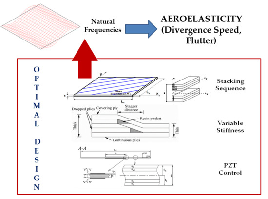
1. Introduction
2. Governing Relations
- –
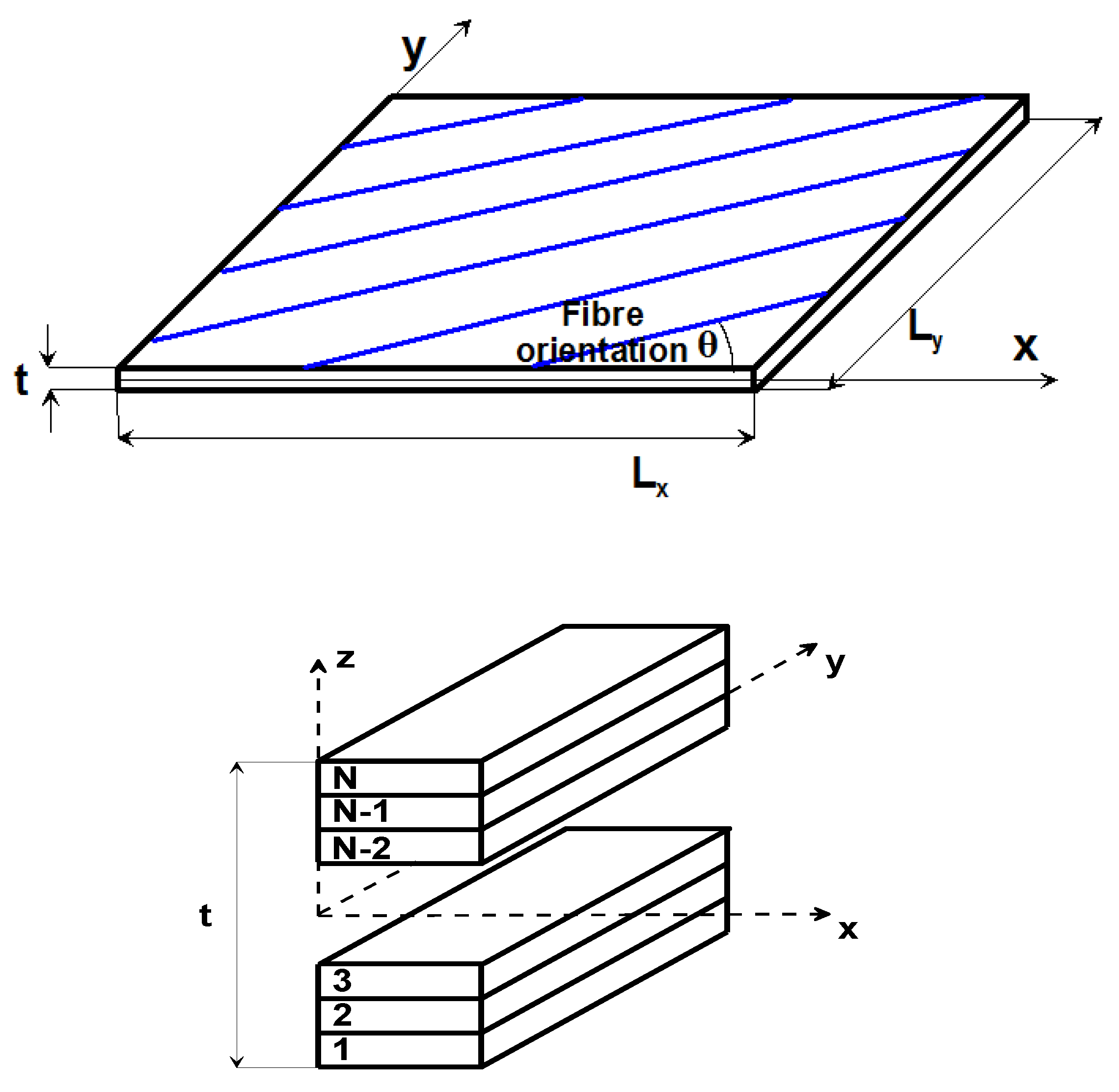
- The plate is constructed of flat, uniform-thickness layers of orthotropic sheets bonded together. The direction of principal stiffness of the individual layers does not in general coincide with the plate edges (see Figure 3). The plate is thin; i.e., the thickness t is much smaller than the other physical dimensions Lx and Ly.
- –
- In the theoretical considerations, the Kirchhoff hypothesis is used, i.e., transverse shear and normal strains are negligible; however, in the finite element analysis, the first-order transverse shear deformation theory is used.
- –
- The thicknesses of individual layers are identical and equal to t/N, where N denotes the total number of plies in the laminate; the distances in the individual laminas are measured from the geometrical mid-plane of the plate.
3. Method of the Solution
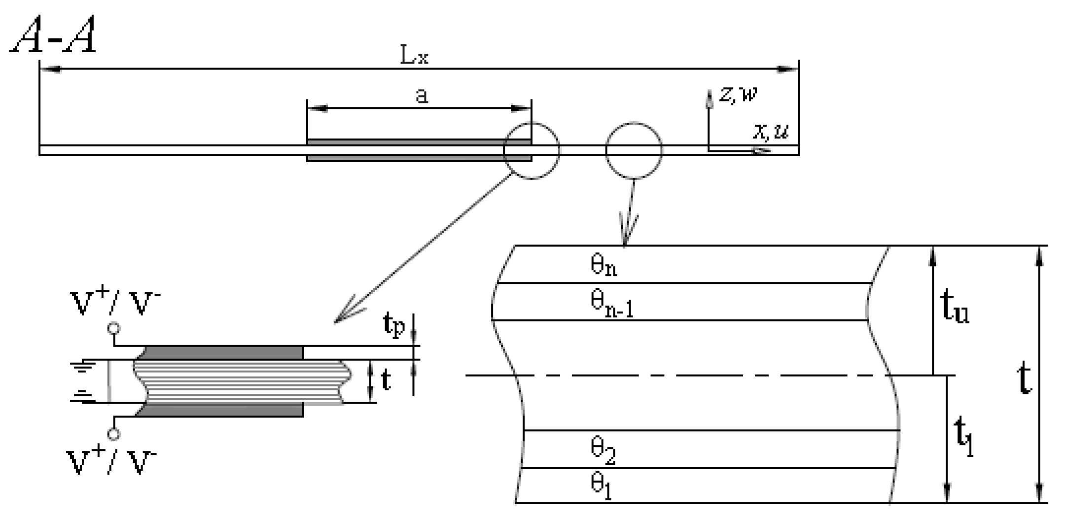
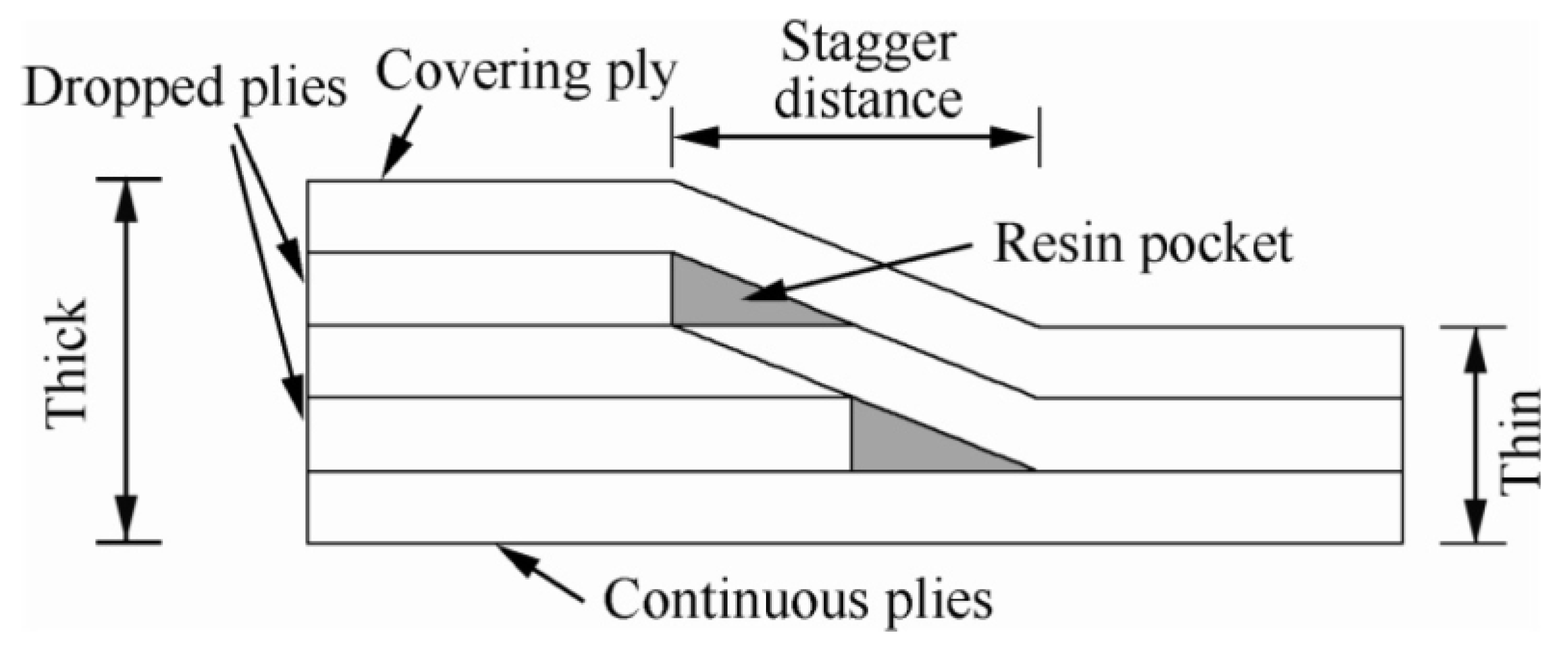
4. Optimal Design
4.1. Definition of Design Variables
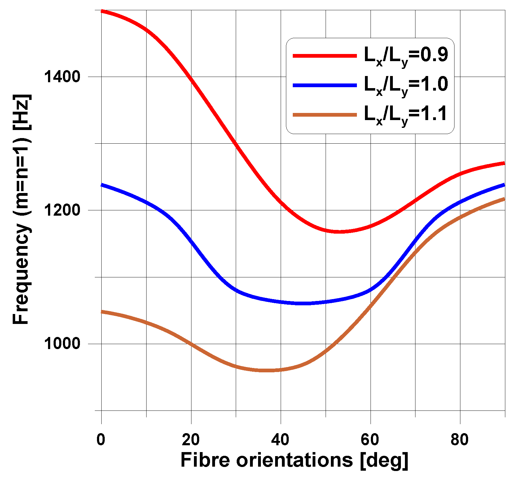
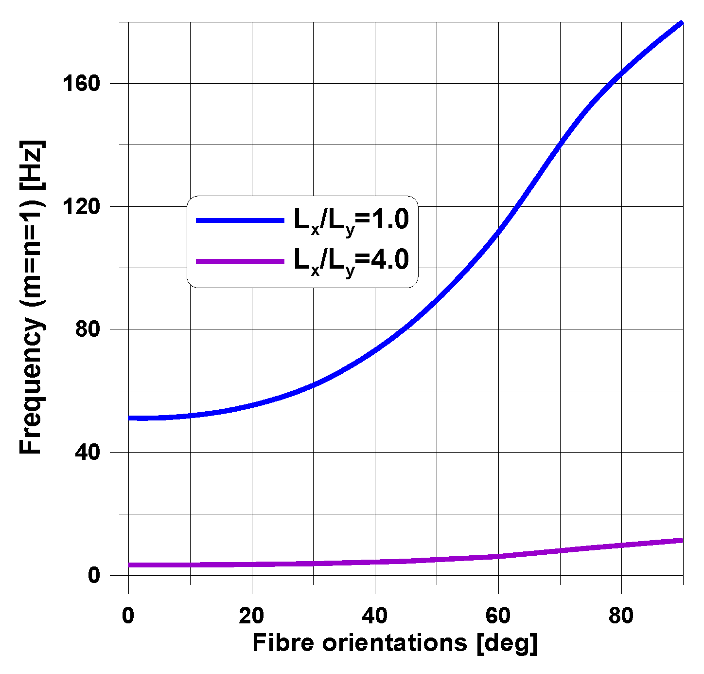
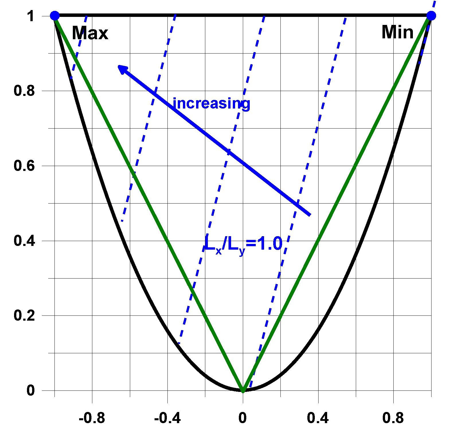
4.2. Optimal Stacking Sequences
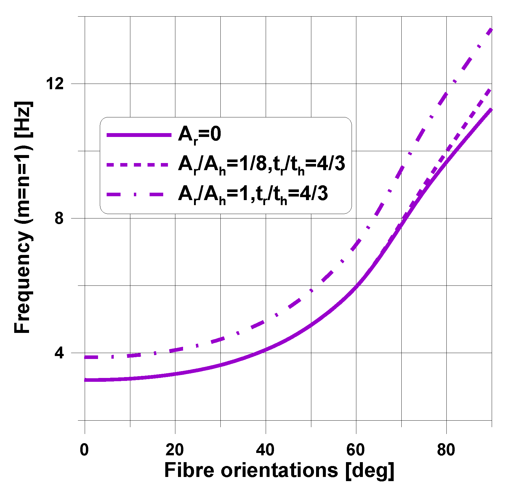
4.3. Variable Stiffness
5. Conclusions
Funding
Conflicts of Interest
Appendix A
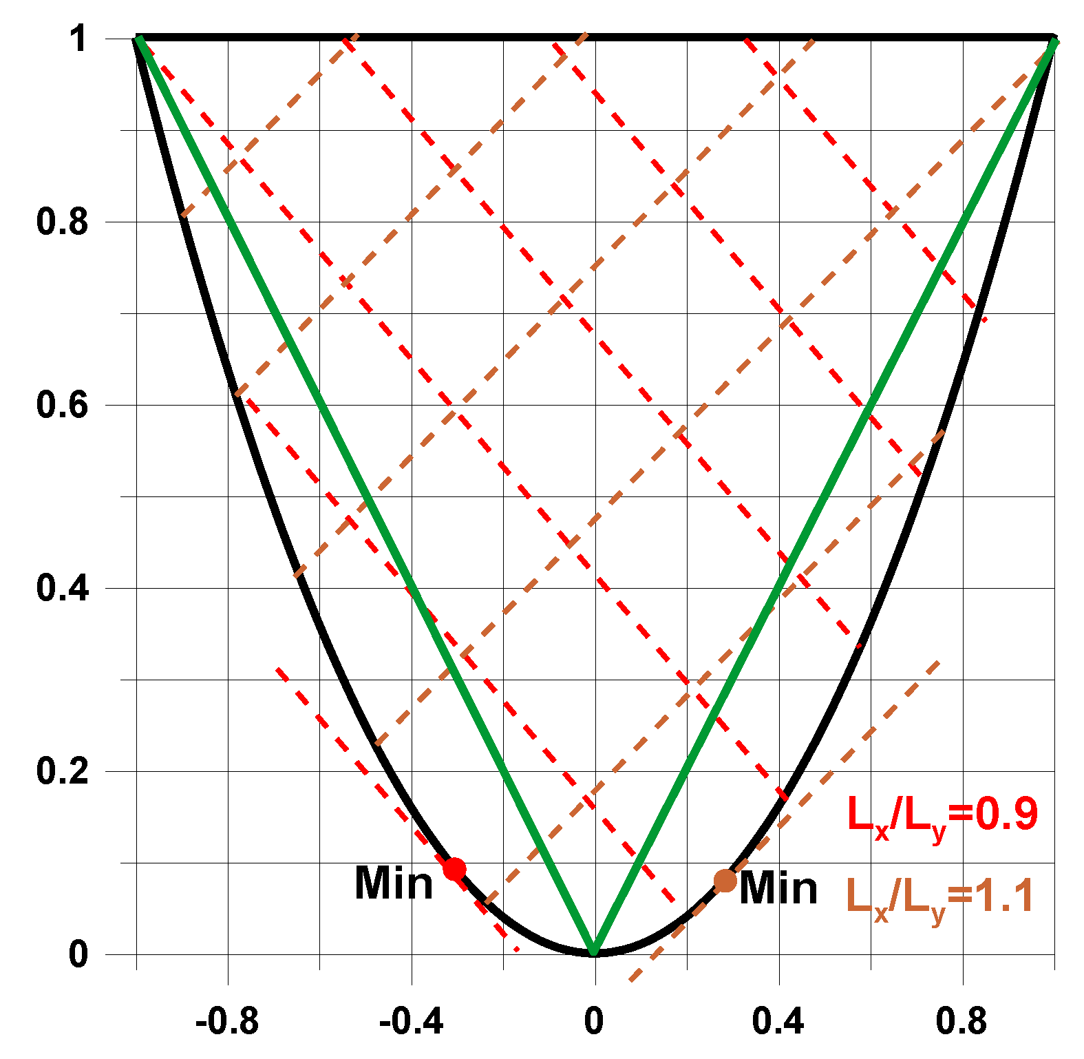
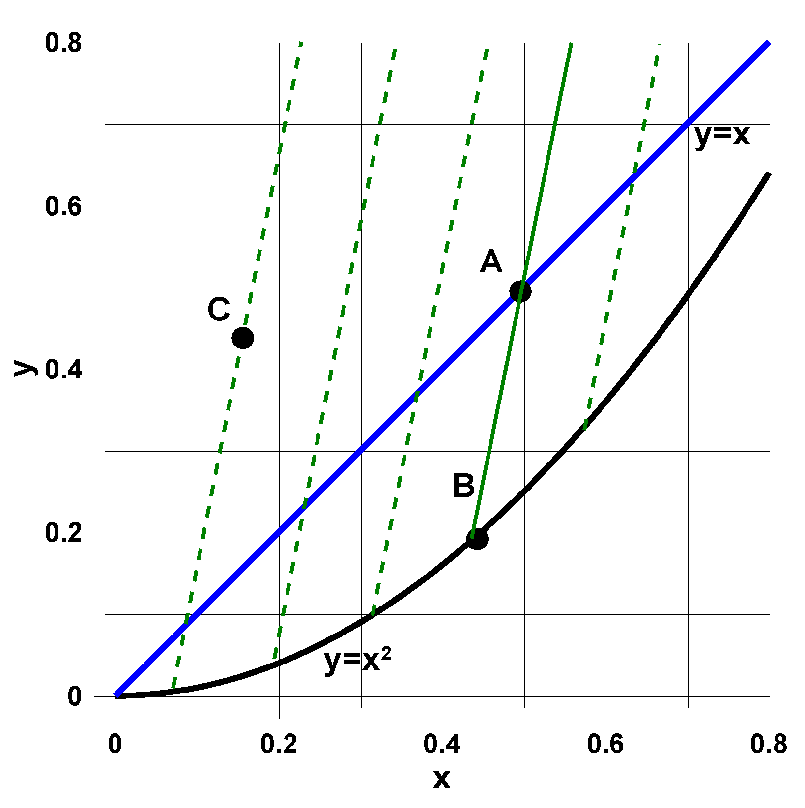
- Choose point A belonging to the edges of the triangle (Figure A1);
- Find the appropriate stacking sequence corresponding to the value xA; the fundamental two operations are given below (the package Mathematica):a = Table[3*l * (l − 1) + 1,{l, N/4}];f = Subsets[a,{L}];
- 3.
- Compute the value of the eigenfrequency corresponding to the assumed stacking sequence—the chosen subset f;
- 4.
- At the design space (x, y), find the point B belonging to the parabola (angle-ply fiber orientations) which has the identical value of the eigenfrequency as that for symmetric laminates corresponding to the subset f and computed at the previous step;
- 5.
- Join the points A and B (Figure A1);
- 6.
- Draw a set of straight lines parallel to the straight line AB;
- 7.
- Choose the appropriate value of the eigenfrequency (the parameter of the parallel lines) and the point C;
- 8.
- Find the stacking sequence corresponding to the point C.

References
- Lovejoy, A.E. Natural Frequencies and an Atlas of Mode Shapes for Generally Laminated, Thick, Skew, Trapezoidal Plates. Master’s Thesis, Virginia Polytechnic Institute and State University, Blacksburg, VA, USA, 1994. [Google Scholar]
- Fantuzzi, N.; Tornabene, F.; Bacciocchi, M.; Ferreira, A.J.M. On the Convergence of Laminated Composite Plates of Arbitrary Shape through Finite Element Models. J. Compos. Sci. 2018, 2, 16. [Google Scholar] [CrossRef]
- Yu, Y.-Y. Vibrations of Elastic Plates: Linear and Nonlinear Dynamical Modeling of Sandwiches, Laminated Composites, and Piezoelectric Layers; Springer: New York, NY, USA, 1996. [Google Scholar]
- Kapania, R.K.; Raciti, S. Recent advances in analysis of laminated beams and plates. Part II: Vibrations and wave propagation. AIAA J. 1989, 27, 935–945. [Google Scholar] [CrossRef]
- Reddy, J.N.; Khdeir, A.A. Buckling and vibration of laminated composite plates using various plate theories. AIAA J. 1989, 27, 1809–1817. [Google Scholar] [CrossRef]
- Tornabene, F.; Fantuzzi, N.; Bacciocchi, M.; Viola, E. Higher-order theories for the free vibrations of doubly-curved laminated panels with curvilinear reinforcing fibers by means of a local version of the GDQ method. Compos. Part B Eng. 2015, 81, 196–230. [Google Scholar] [CrossRef]
- Tornabene, F.; Fantuzzi, N.; Bacciocchi, M. Foam core composite sandwich plates and shells with variable stiffness: Effect of the curvilinear fiber path on the modal response. J. Sandw. Struct. Mater. 2017. [Google Scholar] [CrossRef]
- Grandhi, R. Structural optimization with frequency constraints—A review. AIAA J. 1993, 31, 2296–2303. [Google Scholar] [CrossRef]
- Szyszkowski, W.; King, J.M. Optimization of frequencies spectrum in vibrations of flexible structures. AIAA J. 1993, 31, 2163–2168. [Google Scholar]
- Bert, C.W. Optimal design of a composite material plate to maximize its fundamental frequency. J. Sound Vib. 1977, 50, 229–237. [Google Scholar] [CrossRef]
- Bert, C.W. Design of clamped composite-material plates to maximize fundamental frequency. J. Mech. Des. 1978, 100, 274–278. [Google Scholar] [CrossRef]
- Reiss, R.; Ramachandran, S. Maximum frequency design of symmetric angle-ply laminates. Comput. Struct. 1987, 4, 476–487. [Google Scholar]
- Grenestedt, J.L. Layup optimization and sensitivity analysis of the fundamental eigenfrequency of composite plates. Compos. Struct. 1989, 12, 193–209. [Google Scholar] [CrossRef]
- Wright, J.R.; Cooper, J.E. Introduction to Aircraft Aeroelasticity and Loads; John Wiley & Sons: Chichester, UK, 2007. [Google Scholar]
- Chowdary, T.V.; Sinha, P.K.; Parthan, S. Finite element flutter analysis of composite skew panels. Comput. Struct. 1996, 58, 613–620. [Google Scholar] [CrossRef]
- Forster, E.E.; Yang, H.T. Flutter control of wing boxes using piezoelectric actuators. J. Aircraft 1998, 35, 949–957. [Google Scholar] [CrossRef]
- Moosavi, M.R.; Oskouei, A.N.; Khelil, A. Flutter of subsonic wing. Thin Walled Struct. 2005, 43, 617–627. [Google Scholar] [CrossRef]
- Zhao, H.; Cao, D. A study on the aero-elastic flutter of stiffened laminated composite panel in the supersonic flow. J. Sound Vib. 2013, 332, 4668–4679. [Google Scholar] [CrossRef]
- Alyanak, E.J.; Pendleton, E. A design study employing aeroelastic tailoring and an active aeroelastic wing design approach on a tailless lambda wing configuration. In Proceedings of the 15th AIAA/ISSMO Multidisciplinary Analysis and Optimization Conference, Atlanta, GA, USA, 16–20 June 2014. [Google Scholar]
- Singha, M.K.; Ganapathi, M. A parametric study on supersonic flutter behavior of laminated composite skew flat panels. Compos. Struct. 2005, 69, 55–63. [Google Scholar] [CrossRef]
- Hyer, M.W.; Charette, R.F. Use of curvilinear fiber format in composite structure design. In Proceedings of the 30th Structures, Structural Dynamics, and Material Conference, Mobile, AL, USA, 3–5 April 1989; pp. 1011–1015. [Google Scholar]
- Abdalla, M.M.; Setoodeh, S.; Gurdal, Z. Design of variable stiffness composite panels for maximum fundamental frequency using lamination parameters. Compos. Struct. 2007, 81, 283–291. [Google Scholar] [CrossRef]
- Kameyama, M.; Fukunaga, H. Optimum design of composite plate wings for aeroelastic characteristics using lamination parameters. Compos. Struct. 2007, 85, 213–224. [Google Scholar] [CrossRef]
- Chandra, R.; Chopra, I. Structural modeling of composite beams with induced-strain actuators. AIAA J. 1993, 31, 1692–1701. [Google Scholar] [CrossRef]
- Brunelle, E.J.; Robertson, S.R. Initially stressed mindlin plates. AIAA J. 1974, 12, 1036–1045. [Google Scholar] [CrossRef]
- Yang, I.H.; Shieh, J.A. Vibrations of initially stressed thick rectangular orthotropic plates. J. Sound Vib. 1987, 119, 545–558. [Google Scholar] [CrossRef]
- Rammerstorfer, F.G. Increase of the first natural frequency and buckling load of plates by optimal fields of initial stresses. Acta Mech. 1977, 27, 217–238. [Google Scholar] [CrossRef]
- Shah, P.H.; Ray, M.C. Active control of laminated composite truncated conical shells using vertically and obliquely reinforced 1-3 piezoelectric composites. Eur. J. Mech. A Solids 2012, 32, 1–12. [Google Scholar] [CrossRef]
- Kędziora, P.; Muc, A. Optimal shapes of PZT actuators for laminated structures subjected to displacement or eigenfrequency constraints. Compos. Struct. 2012, 94, 1224–1235. [Google Scholar] [CrossRef]
- Muc, A.; Kędziora, P. Optimal Design of Smart Laminated Composite Structures. Mater. Manuf. Process. 2010, 25, 272–280. [Google Scholar] [CrossRef]
- Muc, A.; Kędziora, P.; Stawiarski, A. Buckling enhancement of laminated composite structures partially covered by piezoelectric actuators. Eur. J. Mech. A Solids 2019, 73, 112–125. [Google Scholar] [CrossRef]
- Mota Soares, C.M.; Mota Soares, C.A.; Franco Correia, V.M. Optimal design of piezolaminated structures. Compos. Struct. 1999, 47, 625–634. [Google Scholar] [CrossRef]
- Ganesan, R.; Zabihollah, A. Vibration analysis of tapered composite beams using a higher-order finite element: I. Formulation. Compos. Struct. 2007, 77, 306–318. [Google Scholar] [CrossRef]
- Ganesan, R.; Zabihollah, A. Vibration analysis of tapered composite beams using a higher-order finite element: II. Parametric study. Compos. Struct. 2007, 77, 319–330. [Google Scholar] [CrossRef]
- Kapania, R.K.; Singhvi, S. Free vibration analyses of generally laminated tapered skew plates. Compos. Eng. 1992, 2, 197–212. [Google Scholar] [CrossRef]
- Viglietti, A.; Zappino, E.; Carrera, E. Free vibration analysis of locally damaged aerospace tapered composite structures using component-wise models. Compos. Struct. 2018, 192, 38–51. [Google Scholar] [CrossRef]
- Muc, A. Design of blended/tapered multilayered structures subjected to buckling constraints. Compos. Struct. 2018, 186, 256–266. [Google Scholar] [CrossRef]
- Babu, A.A.; Vasudevan, R. Vibration analysis of rotating delaminated non-uniform composite plates. Aerosp. Sci. Technol. 2017, 60, 172–182. [Google Scholar] [CrossRef]
- Muc, A. Optimal design of composite multilayered plated and shell structures. Thin-Walled Struct. 2007, 45, 816–820. [Google Scholar] [CrossRef]
- Whitney, J.M.; Leissa, A.W. Analysis of heterogeneous anisotropic plates. ASME J. Appl. Mech. 1969, 36, 261–266. [Google Scholar] [CrossRef]
- Grenestedt, J.L. Layup Optimization of Composite Structures; Report No. 92-24; Royal Institute of Technology: Stockholm, Sweden, 1992. [Google Scholar]
- Li, J.; Narita, Y. Analysis and optimal design for supersonic composite laminated plate. Compos. Struct. 2013, 101, 35–46. [Google Scholar] [CrossRef]
- Miki, M.; Sugiyama, Y. Optimum design of laminated composite plates using lamination parameters. AIAA J. 1993, 31, 921–922. [Google Scholar] [CrossRef]
- Fukunaga, H.; Vanderplaats, G.N. Stiffness Optimization of Orthotropic Laminated Composites Using Lamination Parameters. AIAA J. 1991, 29, 641–648. [Google Scholar] [CrossRef]
- Diaconu, C.G.; Sekine, H. Layup optimization for buckling of laminated composite shells with restricted layer angles. AIAA J. 2004, 42, 2153–2158. [Google Scholar] [CrossRef]
- Diaconu, C.G.; Sato, M.; Sekine, H. Buckling characteristics and layup optimization of long laminated composite cylindrical shells subjected to combined loads using lamination parameters. Compos. Struct. 2002, 58, 423–433. [Google Scholar] [CrossRef]
- Bloomfield, M.W.; Diaconu, C.G.; Weaver, P.M. On feasible regions of lamination parameters for lay-up optimization of laminated composites. Proc. R. Soc. A Math. Phys. Eng. Sci. 2009, 465, 1123–1143. [Google Scholar] [CrossRef]
- Muc, A. Choice of design variables in the stacking sequence optimization for laminated structures. Mech. Compos. Mater. 2016, 52, 211–224. [Google Scholar] [CrossRef]
- Muc, A.; Chwał, M. Analytical discrete stacking sequence optimization of rectangular plates subjected to buckling and FPF constraints. J. Theor. Appl. Mech. 2016, 54, 423–436. [Google Scholar] [CrossRef]
- NISA II User’s Manual; Engineering Mechanics Research Corporation: Troy, MI, USA, 1993.
- Muc, A.; Ulatowska, A. Local fibre reinforcement of holes in composite multilayered plates. Compos. Struct. 2012, 94, 1413–1419. [Google Scholar] [CrossRef]
- Muc, A.; Muc-Wierzgoń, M. An evolution strategy in structural optimization problems for plates and shells. Compos. Struct. 2012, 94, 1461–1470. [Google Scholar] [CrossRef]
- Muc, A.; Muc-Wierzgoń, M. Discrete optimization of composite structures under fatigue constraints. Compos. Struct. 2015, 133, 834–839. [Google Scholar] [CrossRef]
- Muc, A. Evolutionary design of engineering constructions. Latin Am. J. Solids Struct. 2018, 15, 87. [Google Scholar] [CrossRef]
- Muc, A. Peculiarities in the material design of buckling resistance for tensioned laminated composite panels with elliptical cut-outs. Materials 2018, 11, 1019. [Google Scholar] [CrossRef] [PubMed]


© 2018 by the author. Licensee MDPI, Basel, Switzerland. This article is an open access article distributed under the terms and conditions of the Creative Commons Attribution (CC BY) license (http://creativecommons.org/licenses/by/4.0/).
Share and Cite
Muc, A. Natural Frequencies of Rectangular Laminated Plates—Introduction to Optimal Design in Aeroelastic Problems. Aerospace 2018, 5, 95. https://doi.org/10.3390/aerospace5030095
Muc A. Natural Frequencies of Rectangular Laminated Plates—Introduction to Optimal Design in Aeroelastic Problems. Aerospace. 2018; 5(3):95. https://doi.org/10.3390/aerospace5030095
Chicago/Turabian StyleMuc, Aleksander. 2018. "Natural Frequencies of Rectangular Laminated Plates—Introduction to Optimal Design in Aeroelastic Problems" Aerospace 5, no. 3: 95. https://doi.org/10.3390/aerospace5030095
APA StyleMuc, A. (2018). Natural Frequencies of Rectangular Laminated Plates—Introduction to Optimal Design in Aeroelastic Problems. Aerospace, 5(3), 95. https://doi.org/10.3390/aerospace5030095