Abstract
The influence of model deformation needs to be corrected before the aerodynamic force data measured in the wind tunnel is applied to aircraft design. In order to obtain the aerodynamic forces on rigid model shape, this paper presents a fast correction method by establishing a mathematical modelling method connecting aerodynamic forces and wing section torsion. The aerodynamic force coefficients on rigid model shape can then be calculated quickly just by setting section torsion to zero. A 25-point simulation dataset of the High Reynolds Number Aero-Structural Dynamics (HIRENASD) model generated by Computational Fluid Dynamics (CFD) and Static Computational Aeroelasticity (CAE) approach is used to investigate the influence of section locations, basis function type, support radius, and deformation perturbation on the prediction accuracy. Finally, the present correction method is applied to predict the aerodynamic forces on the rigid shape of a NASA common research model. The results of parametric analysis and application show that the present correction method with the Wendland’s C6 function and a support radius of 1.0 can provide a reasonable prediction of aerodynamic forces on the rigid model shape.
1. Introduction
With the increasing competition in the civil aviation market and the effects of global environmental pollution, the manufacturers of modern commercial airplanes prefer light-weight designs with low aerodynamic drag in order to improve the fuel efficiency as well as reduce the emissions [1]. Accurate aerodynamic data plays a significant role in designing a good aircraft. Wind tunnels are still the main experimental facility used to obtain the aerodynamic characteristics of an aircraft. For most regular wind tunnel tests, the aircraft designers think the measured force data is about the rigid shape under the hypothesis that the structure does not deform under aerodynamic loads or the deformation is so small that the influence can be ignored [2].
However, the influence of wing structural deformation on wind tunnel test data must be taken into consideration in some cases [3]. Firstly, the modern transport aircraft usually adopts layout with a large aspect-ratio as well as a swept wing. The wing bending will induce a negative wing section torsion due to the sweep angle of the wing elastic axis [4]. The induced wing section torsion will decrease the local angle of attack to which the aerodynamic force is extremely sensitive. In the transonic wind tunnel test of the DLR-F6 model, a configuration designed and tested by Deutschen Zentrums für Luft- und Raumfahrt (DLR), the wing tip torsion is up to −0.4° at low flow dynamic pressure [5]. In addition, the decrease in drag coefficient caused by model deformation is up to 10 drag counts [6]. Besides, in high Reynolds number wind tunnel tests, the flow dynamic pressure is often very high to obtain high . As a result, model deformation is obvious because of increasing aerodynamic loads [7]. Many published researches have demonstrated that the effects of model deformation and Reynolds number on the aerodynamic force coefficients have the same magnitude, but the influences are opposite [8,9]. In most conditions, model deformation will mask the influence of Reynolds number and cause a pseudo-Reynolds number effects [7]. This will bring a potential risk to the aircraft design if the aerodynamic characteristics at flying Reynolds number are not predicted accurately. A typical case is that the wing structure of the military C-141 transport was redesigned since the aerodynamic forces at flying Reynolds number were seriously underestimated [10].
Moreover, the shape inconsistency induced by model deformation causes a great discrepancy between the numerical prediction and experimental data, which has long influenced the development of verification and validation of Computational Fluid Dynamics (CFD) [11,12]. A Drag Prediction Workshop (DPW) has become one the most prestigious activities in evaluating state-of-the-art of CFD software around the world [13]. However, during the fourth and fifth DPW where the common research model (CRM) was selected as the computational case [14,15], the discrepancy between numerical and experimental data does not decrease when the number of grid cells increases. Rivers and Hue have noticed this phenomenon and used a numerical approach to investigate it [16,17]. They found that the model deformation has a significant influence on the aerodynamic moment. In order to eliminate the influence of model deformation and improve the consistency between numerical and experimental results, the organizing committee of DPW IV published a series of CFD computational grids with different deformed wing shapes [18,19].
Thus, before applying the wind tunnel test data to aircraft design, it is necessary to correct the model deformation effects. Now, there are three kinds of methods to obtain the aerodynamic forces on rigid model shape. The first method is to use test data at different dynamic pressures to extrapolate the data at zero dynamic pressure where the aircraft model has no deformation [20,21,22]. This type of test requires the wind tunnel to be able to adjust the temperature and pressure independently. Only several facilities all over the world, such as European Transonic Windtunnel (ETW), National Transonic Facility (NTF), have such ability [23,24]. However, the test condition is limited by the strength of model material. Another method is based on the computational aeroelasiticity approach to determine the influence of model deformation [25,26,27]. Although the computational aeroelasticity method has been widely used in aircraft design [28,29], there are still some problems predicting the model deformation and variation of aerodynamic force coefficients accurately [19,30]. The third method is a combination of CFD and model deformation measurement (MDM) [31]. MDM firstly measures the model deformation and constructs the deformed model shape. Then, CFD calculates the aerodynamic forces on the rigid and the elastic shape to determine the variation of the forces. Finally, the test data is corrected to aerodynamic forces on the rigid shape. NASA has been developing MDM technology since the 1980s and many high-precision MDM tools have been applied in wind tunnel tests [32]. The third combined method is of high fidelity and can be applied to most wind tunnels in the world. It is an extremely promising alternative for the correction of model deformation effects. In spite of having many advantages, the combined method still needs a lot of computation resources to obtain the CFD results on deformed and non-deformed shape, which leads to costly computation.
In this paper, a fast correction method of model deformation effects by establishing a mathematical modelling method connecting aerodynamic forces and wing section torsion is presented. In Section 2, the construction of the fast correction method through the use of radial basis function interpolation is introduced. In Section 3, the effects of parameters on prediction accuracy are investigated through numerical simulation datasets. In Section 4, the fast correction method is applied to predict the aerodynamic forces on the rigid shape of a NASA CRM model based on the deformation and forces measurement data in ETW.
2. Fast Correction Methods
2.1. Introduction to Method
Aerodynamic forces on wind tunnel model can be determined as long as the running parameters of wind tunnel and the model shape are fixed. Therefore, the aerodynamic force coefficients can be expressed as
where represents the aerodynamic force coefficients of the wind tunnel model; is the flow parameter set, including Mach number, Reynolds number, etc., is the position parameter set, including angle of attack, sideslip angle, roll angle, etc., is the deformation parameter set, including wing bending and wing section torsion. Function f is the relationship between and .
The idea of the fast correction method is to first establish the function between and based on force and deformation data. Then, the aerodynamic force coefficients can be obtained by setting the model deformation to zero, shown as follows:
where is the aerodynamic force coefficients on the rigid model shape.
2.2. Parametric Description of Wing Deformation
Since the deformation of the model mainly happens on the wing, the wing deformation is used to respresent model deformation in this paper. The key objective of the fast correction method is to establish the relationship between aerodynamic force coefficients and wing deformation parameters. Therefore, it is necessary to describe the wing deformation using a finite number of parameters rather than bending and torsion at all wing sections. For a large aspect-ratio wing, the structural deformation is similar to that of a cantilever beam. In beam theory, the deformation under load at a fixed point can be described by a cubic spline. Thus, a high order polynomial can be used to parameterize the wing deformation.
Figure 1 shows the polynomial fitting of bending and torsion of a large aspect ratio wing. In Figure 1, and are wing bending at the trailing edge and wing section torsion, respectively; , which equals , is the normalized spanwise location; wing deformation data is from static aeroelasiticity computation results of the wing in a real flow condition.
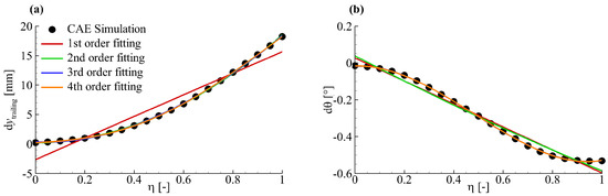
Figure 1.
Polynomial fitting of bending and torsion of a large aspect ratio wing: (a) bending at trailing edge; (b) wing section torsion.
From Figure 1, it can be concluded that a 2nd or higher order polynomial fitting can obtain enough accurate data for wing bending while a third or higher order polynomial fitting is essential to obtain enough accurate data for wing section torsion. This means that the third order polynomial fitting is accurate enough to describe the structural deformation of a large aspect ratio wing. As a result, the wing bending and section torsion can be expressed as
In Equation (3), there are four unknown coefficients in bending or torsion expression which need four section data to be determined. Thus, the wing deformation parameter set can be written as
2.3. Modelling of Aerodynamic Forces
In present paper, the aerodynamic force model is based on the longitudinal aerodynamic force data from one single wind tunnel test where wing deformation changes with angle of attack while the other parameters remain constant. So Equation (5) can be expressed as
Besides, pure wing bending has little influence on longitudinal aerodynamic force coefficients. Thus, we can neglect the effect of wing bending and Equation (6) can be approximately expressed as
Defining wing section angle of attack as
The geometric angle of attack, , which equals the angle of attack of the wing root section, can also be determined by the angle of attack at four wing sections: . Therefore, Equation (9) can be changed into
In Equation (10), for a single wind tunnel test with only the angle of attack varying, the longitudinal aerodynamic force coefficients can be expressed as the function of the angle of attack at the four wing sections.
Radial basis function interpolation (RBF), which has a good precision in describing continuous functions, can transform a multivariate interpolation into an univariate problem through the basis function. Therefore, the present paper aims at establishing the relationship between and wing section angle of attack by the use of RBF. In RBF form [33], Equation (10) is expressed as
where N is the number of total sample data; are the interpolation coefficients; is the basis function; the independent variable is defined as ; the distance is calculated as
On the basis of the N sample data , linear equations about coefficients through Equation (11) can be constructed.
where . By solving the linear equations, the interpolation coefficients are obtained, shown as follows:
Substituting Equation (14) into Equation (11) yields
where . The prediction accuracy of Equation (15) is dependent on the types of basis function. The basis function in RBF may be divided into three types: global, local, and compact [34]. Global functions remain non-zero and grow as the independent variable increases. Local functions also remain non-zero but decay as the independent variable increases. Compact functions are similar to local functions, decaying as the independent variable increases, but reach zero at some finite distance, termed support radius. More details about the basis function in RBF can be obtained from Buhmann [35].
Table 1 gives some common basis functions in RBF interpolation. In Table 1, c is a free parameter; , in which R is the support radius. For compact basis functions, equals zero when distance x is larger than the support radius R. This means that the contribution of sample point is strictly limited in the radius R. In the next section, the influence of the basis function type and support radius is investigated through a large aspect-ratio wing case.

Table 1.
Common basis function in RBF interpolation.
There are some free parameters in the basis function, such as the support radius. In practice, the wing section angle of attack in Equation (15) is often normalized between 0 and 1 so that the parameters selection in RBF can be used for different cases. The normalization angle of attack can be written as
where , are the minimum and maximum angles of attack, respectively.
2.4. Correction of Model Deformation Effects
From Equation (15), the value of aerodynamic force coefficients at any can be calculated directly. For rigid model shape, the wing section torsion is zero. As a result, the parameter of rigid shape is . The aerodynamic force coefficients on the rigid model shape can be obtained by subsituting this value of into Equation (15), shown as follows:
where .
The main time cost for the aerodynamic force modelling method is in solving the linear equations related to the interpolation coefficients . The time cost is less than 1 s, which can be ignored compared to CFD simulation time, when the number of sample data N is less than 100. As a result, the present method can immediately obtain the aerodynamic force coefficients on the rigid model shape as soon as the force and deformation are measured in the wind tunnel.
In the present paper, the effect of wing geometric twist has not been taken into consideration in calculating the local wing section angle of attack in the aerodynamic force modelling method. In fact, this effect is zero since the geometric twist of wing sections remains constant in wind tunnel test and will be eliminated in calculating the value of the basis function.
3. Parametric Analysis
From the description of the fast correction method in Section 2, it can be seen that the accuracy of the present method is dependent on some parameters, such as selection of wing sections, types of basis function, and the support radius in compact basis functions. Thus, the influence of these parameters on the correction results is investigated through a large aspect-ratio wing model in this section. Since there is not enough experimental aerodynamic force or deformation data to support the parametric analysis, CFD and Computational Aeroelasticity (CAE) methods are used to provide the sample and verification data for the aerodynamic force modelling.
In the following subsection, the large aspect-ratio wing model is first introduced. Then the CFD and CAE solvers used in this paper are briefly described and a validation case is provided to demonstrate the accuracy of the coupling solver. In Section 3.3, a modelling case is presented to provide comparison data for the parametric analysis. In Section 3.4, Section 3.5, Section 3.6 and Section 3.7, the effects of wing section location, basis function type, support radius, and deformation perturbation on the results of aerodynamic force modelling are investigated, respectively.
3.1. HIRENASD Model
The High Reynolds Number Aero-Structural Dynamics (HIRENASD) wing model is selected as the research model in this section. The HIRENASD wing is a benchmark case in the first AePW (Aeroelastic Prediction Workshop) [36]. Figure 2 gives some information of the HIRENASD wing model. In a wind tunnel test, a pseudobody was installed to eliminate the boundary effects of the wind tunnel wall. But the wing and the body were not connected and the balance only measured the aerodynamic force on the wing. More details about the HIRENASD wing can be found in Ballmann [20].
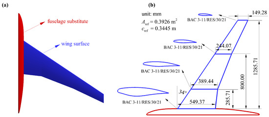
Figure 2.
The High Reynolds Number Aero-Structural Dynamics (HIRENASD) wing model: (a) wing shape; (b) geometry information [37].
3.2. CFD and CAE Solvers
In this paper, an in-house CFD flow solver Trisonic Platform (TRIP), which has been developed by the China Aerodynamics Research and Development Center (CARDC) since the late 1990s, is used to obtain aerodynamic forces on the rigid shape. TRIP is a cell-center-based, finite-volume, Euler/RANS and multiblock grid flow solver. There are different spatial discretization and time integration schemes in TRIP. In this paper, Reynolds Average Navier-Stokes (RANS) equations are used. A second-order Roe scheme is used for the inviscous term discretization and a second-order central scheme is used for the viscous term discretization. The Menter’s SST model [38] is used for the turbulence simulation. The Lower-Upper Symmetric Gauss-Seidel (LU-SGS) scheme [39] is used for the time integration. Multigrid and MPI-based parallel technology are used to accelerate the convergence speed.
The CAE solver used in this paper was developed based on the flow solver TRIP. A flexibility matrix method is used to calculate the wing deformation. The Thin Plate Spline (TPS) interpolation is used to exchange the aerodynamic forces and structural deflection between different solvers. A combined dynamic grid method based on RBF and Transfinite Interpolation (TFI) is used to update the CFD grid after wing deforms. A weak coupling scheme is used to couple flow and structure solver.
The CFD and the CAE solver used in this paper have been validated in many cases, including the HIRENASD wing. A coupling case of the HIRENASD wing, which is used in Reimer [40], is provided to demonstrate the solver accuracy. Table 2 gives the computational parameters of the HIRENASD wing in the validation case. In Table 2, is the nondimensional loading factor, in which q is the dynamic pressure of farfield flow and E is Young’s module of the wing material.
Table 2.
Computational parameters of the HIRENASD wing in the validation case.
Figure 3 gives the CFD grid used in this validation case. This multiblock grid is generated by the AePW organizing committee and provided to submitters to use in the first AePW. There are 319 blocks, 3,158,849 grid nodes, and 3,088,384 grid cells in this grid. An O-type grid is generated around the wing and body to simulate the boundary flow. The thickness of the first layer is 4.4 × 10⁻⁷ m, and the corresponding is 0.66 for of 1.4 × 10⁷. This CFD grid can be downloaded from the AePW website where more information about this grid is provided. In the following parametric analysis, this CFD grid continues to be used to obtain aerodynamic forces on rigid and elastic shape.
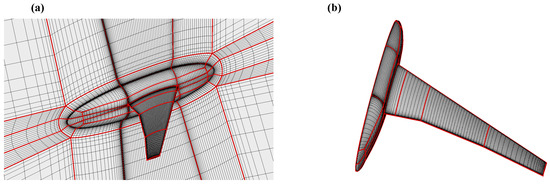
Figure 3.
Computational Fluid Dynamics (CFD) computational grid of HIRENASD wing model: (a) grid topology; (b) surface grid.
The finite element model of the HIRENASD wing is also obtained from the AePW website. Then, a reduced flexibility matrix [37] is extracted from the finite element model and used for the calculation of the wing deformation. Figure 4 gives the wing tip deformation of the HIRENASD model by different methods. In Figure 4, we can see the SOFIA data represents the results from the CAE package, which is developed and used in Aachen University, Germany.The deformation data of ETW and SOFIA in Figure 4 was extracted from Reimer [40]. The good consistency among the wing deformation results of ETW, TRIP, and SOFIA indicates that the TRIP solver used in this paper can provide accurate data for the parametric analysis of the aerodynamic force modelling.
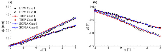
Figure 4.
Wing tip deformation of the HIRENASD model: (a) deflection; (b) torsion.
In the following parametric analysis, the CAE solver is used to calculate the aerodynamic forces on the elastic shape and wing deformation, which are used as sample data of aerodynamic force modelling. The CFD solver is used to provide aerodynamic forces on the rigid shape, which are used to check the results of aerodynamic force modelling.
3.3. Modelling Case
The computational parameters for the modelling case are: Mach number is 0.80; Reynolds number is 7.0 × 10⁶; model angle of attack ranges from −2° to 4°; loading factor is 2.2 × 10⁻⁷. The aerodynamic forces and wing deformation are calculated per 0.25° interval of angle of attack, so there are a total of 25 sample data points for aerodynamic force modelling.
In this modelling case, four wing sections, which are isometrically distributed from wing root to wing tip, are selected. Figure 5 shows the selection scheme of wing sections and torsion angle of these sections.
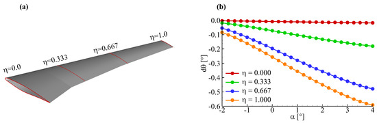
Figure 5.
Selection scheme of wing sections and torsion: (a) section locations; (b) torsion angle.
Figure 6 gives the aerodynamic force modelling results for the HIRENASD wing model. In Figure 6, ‘Rigid’ represents aerodynamic force coefficients of rigid shape, which are used to evaluate the precision of modelling; ‘Elastic’ represents aerodynamic force coefficients of elastic shape, which provide the sample data for the modelling; ‘modelling’ represents aerodynamic force coefficients predicted by modelling method. In this case, the Wendland’s C6 function is selected as the basis function and a support radius is used.
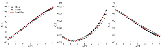
Figure 6.
Aerodynamic force modelling results for HIRENASD wing model: (a) ; (b) ; (c) .
3.4. Effects of Wing Section Location
In Equation (3), bending and torsion are evaluated at four different wing sections to determine the coefficients of cubic polynomial and calculate the torsion at any spanwise location. Figure 7 shows four different selection schemes of wing sections. Scheme I has the same wing section selection as the modelling case in Section 3.3. The wing sections in scheme I to scheme III are isometrically distributed but the distance between the two adjacent wing sections decreases from scheme I to scheme III. Scheme IV is an area-based selection where each wing section has the same projected wing area in the plane .
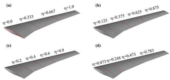
Figure 7.
Different selection schemes for wing section: (a) scheme I; (b) scheme II; (c) scheme III; (d) scheme IV.
Figure 8 shows the aerodynamic force modelling results for the HIRENASD wing with different selection schemes of wing sections. All the modelling parameters in Figure 8 are the same as that in modelling case in Section 3.3, except the wing section location. Here, the instead of absolute value of is used to evaluate the precision of aerodynamic force modelling since the variation of induced by wing deformation is a small value relative to absolute . The is defined as
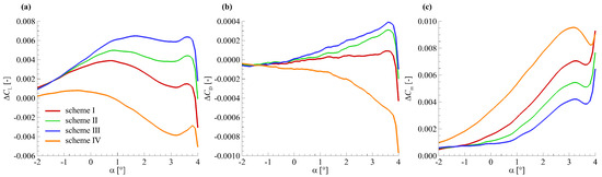
Figure 8.
Aerodynamic force modelling results for HIRENASD wing with different selection schemes of wing sections: (a) ; (b) ; (c) .
A smaller value of indicates a better prediction of the aerodynamic modelling. There is a total of 25 aerodynamic force data points on the rigid model shape obtained by the CFD solver. In order to show more detail information of the , a cubic spline interpolation is used to obtain aerodynamic force data per 0.1° from −2° to 4°. Thus, there are 61 data points in Figure 8. As a result, the data in Figure 8 is shown as smooth solid lines instead of discrete points.
Figure 8 shows: (a) aerodynamic force modelling with selection scheme I, II, III all overestimated the value of , , ; the and increases from selection scheme I to scheme III while decreases; (b) aerodynamic force modelling with section selection scheme IV underestimated the and and overestimated the ; (c) the and obtained by scheme IV are much larger than that from the other three selection schemes. Figure 8 shows that the isometric section selection has better modelling results than the equal-area based scheme.
3.5. Effects of Basis Function Type
In this subsection, the effects of basis function type on aerodynamic force modelling are evaluated. Six basis functions were selected for comparison. These basis functions involve four compact Wendland’s functions (C0, C2, C4, C6) and two globe basis functions (Thin Plate Spline, Volume Spline). Figure 9 shows the aerodynamic force modelling results for the HIRENASD wing model with the six different basis functions. All the modelling parameters in Figure 9 are the same as that in modelling case in Section 3.3, except the basis function type.
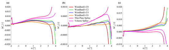
Figure 9.
Aerodynamic force modelling results for HIRENASD wing model with different basis functions: (a) ; (b) ; (c) .
Figure 9 shows that all these six basis functions have good aerodynamic force modelling results when the geometry angle of attack is less than 3°. For larger than 3°, aerodynamic forces from modelling with the C0, C2, TPS, and VS basis functions have an obvious discrepancy with force data of rigid shape. For all angles of attack, Wendland’s C4 and C6 functions can provide good aerodynamic force coefficients of rigid shape.
3.6. Effects of Support Radius
The compact Wendland’s C6 basis function is used to investigate the effects of support radius on aerodynamic force modelling results. All parameters are the same as that in the modelling case in Section 3.3, except the support radius.
Figure 10 shows aerodynamic force modelling results for the HIRENASD wing model with different support radius values. It is shown in Figure 10 that the aerodynamic force modelling results at R = 1.0 are better than the data at the other R values. For a small value of R, the contribution of a sample data is also limited in a small range according to the definition of the support radius. Then, the number of the sample data points, which contributes to evaluating the aerodynamic forces on the rigid shape at an angle of attack, decreases. This will cause accuracy loss when the R is extremely small. However, for a very large value of R, all the sample data are used to evaluate the aerodynamic forces on the rigid shape at an angle of attack. This may bring a local error related to the sample data into the calculation of the aerodynamic forces on the rigid shape and cause a large discrepancy. The results shown in Figure 10 indicate that a value of R close to 1.0 can provide better prediction results.
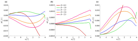
Figure 10.
Aerodynamic force modelling results for the HIRENASD wing model with different support radius values: (a) ; (b) ; (c) .
3.7. Effects of Deformation Perturbation
In model deformation measurements in wind tunnel tests, there might be oscillation of wing section torsion due to the influence of some factors, such as vibration of the model and cameras. In this subsection, the effects of deformation perturbation on aerodynamic force modelling are investigated. The perturbation of wing section torsion is added by the use of random number generated in program, defined as
where is the perturbation of wing section torsion; is the random number, which ranges from −1.0 to 1.0; is the amplitude of perturbation. Thus, the wing section torsion after perturbation is
Figure 11 shows the wing section torsion with and without perturbation. Here, the amplitude of perturbation is 10.0%. ‘-’ in Figure 11 represents the three-order polynomial fitting of wing section torsion with perturbation.
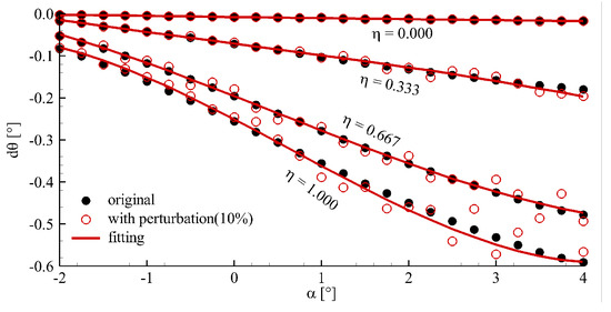
Figure 11.
Wing section torsion with and without perturbation.
Figure 12 shows the aerodynamic force modelling results for the HIRENASD wing model with different perturbations. Results indicate that increases quickly as increases, even for very small perturbation values. However, when is larger than 2.0%, changes little as increases. The results in Figure 12 demonstrate that the aerodynamic force modelling method is extremely sensitive to the perturbation of wing section torsion. Moreover, the influence of perturbation on the modelling results is large enough and we need take into account the influence when modelling the aerodynamic forces.
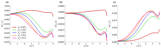
Figure 12.
Aerodynamic force modelling results for the HIRENASD wing model with different perturbations: (a) ; (b) ; (c) .
Figure 13 shows the aerodynamic force modelling results for the HIRENASD wing model with smoothed wing section torsion. Here, the wing section torsion from the three-order polynomial fitting is used, as shown in Figure 11. Figure 13 shows that the aerodynamic force modelling method with different perturbations of section torsion gets nearly the same results after smoothing the torsion angle of wing section. This means that the smoothing can effectively reduce the influence of perturbation.
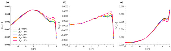
Figure 13.
Aerodynamic force modelling results for the HIRENASD wing model by smoothing the wing section torsion: (a) ; (b) ; (c) .
4. Application
In this section, the present fast correction method is applied to predict the aerodynamic forces on the rigid shape of the NASA CRM model.
4.1. NASA CRM Model
The NASA CRM model is a general wide-body commercial transport configuration designed for evaluating state-of-the-art of CFD software development around the world. This model has been selected as the benchmark case in DPW IV [14], DPW V [15], and DPW IV [18]. Figure 14 shows the shape and geometry parameters of the wind tunnel test model of CRM wing/body/tail configuration, which is used in this paper. More geometry details of CRM model can be found in Vassberg [41] or from NASA’s website [42].
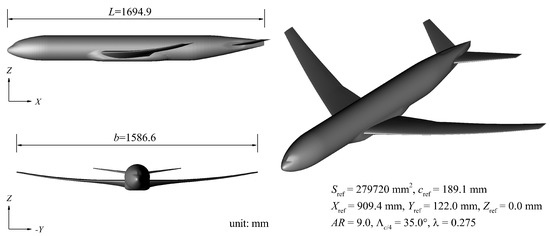
Figure 14.
Geometry parameters of Common Research Model (CRM) wing/body/tail configuration.
4.2. Experimental Data of CRM Model
The CRM model has been tested in Langley’s NTF [43], Ames 11-ft transonic wind tunnel [44], ETW [45], JAXA wind tunnel [46], ONERA-S1MA [47]. These tests provide different types of experimental data, such as aerodynamic force and moment, wing deformation, surface pressure, and flow structure visualization. In this paper, the force, moment, and deformation data of the CRM model obtained in ETW are used for aerodynamic force modelling. These experimental data can be downloaded from the website of the European Strategic Wind Tunnels Improved Research Potential (ESWIRP) [48], which sponsored the wind tunnel tests of CRM model in ETW.
Two cases are selected for use in this section from the available data. Table 3 gives the parameters of the two selected cases. In Table 3, is the serial number of the wind tunnel test in which model deformation are measured. is the serial number of wind tunnel test in which aerodynamic forces are obtained. q is the flow dynamic pressure and E is the Young’s module of the material of which the wind tunnel model is made. The ratio is called loading factor, which is used to describe the magnitude of wing structure deformation under aerodynamic loads.
Table 3.
Selected cases of CRM-WBT model in ETW.
Figure 15 gives the wing section torsion of the NASA CRM-WBT model obtained in ETW. Sections = 0.11, = 0.40, and = 0.70, = 1.00 were selected, which were nearly isometrically distributed along wing span. Figure 15 shows that there are small oscillations of wing section torsion for both cases when the angle of attack is larger than 3°. In Section 3.7 it is demonstrated that deformation perturbation has an important influence on the aerodynamic force modelling. In order to avoid this influence, a three-order polynomial fitting is implemented to obtain smooth wing section torsion at different angles of attack. According to the parametric analysis results, Wendland’s C6 is selected as the basis function of RBF and a support radius of 1.0 is used in this application case.
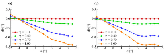
Figure 15.
Wing section torsion of NASA Common Research Model (CRM) wing/body/tail configuration: (a) case I; (b) case II.
4.3. Pseudo-Experimental Forces on the Rigid Shape
In this section, a method, which uses experimental forces at different loading factors to correct the influence of wing deformation, is adopted to provide experimental forces on the rigid shape for comparison. Since this method does not directly measure the forces on the rigid shape in wind tunnel tests, so the obtained forces are called the pseudo-experimental forces on the rigid shape, marked as ‘Pseudo Rigid’.
The method to obtain the ‘Pseudo Rigid’ data is briefly introduced in the following. Firstly, the variation of aerodynamic forces induced by wing deformation can be expressed as
where is the aerodynamic force coefficients of the elastic shape at loading factor ; is the aerodynamic force coefficients of the rigid shape; is the variation of induced by wing structural deformation at loading factor . The relationship between the and the loading factor is nearly linear. Therefore, the can be calculated by linear extrapolation of force data on the elastic shape at different loading factors .
In wind tunnel tests, Reynolds number always varies when the loading factor changes. In this paper, the influence of variation of Reynolds number on the wing deformation and the is ignored. Thus, the aerodynamic force coefficients data of elastic shape at different Reynolds numbers can be used in Equation (23) to calculate the . Two experimental data at = 19.8 × 10⁶, in which the loading factors are 3.342 × 10⁻⁷ and 5.058 × 10⁻⁷, respectively, are used in this application case. The run serial numbers of wind tunnel tests of the two experimental data are 227 and 218, respectively. More detailed information about the two experimental data sets can be obtained from the ESWIRP’s website.
4.4. Results and Discussion
Figure 16 and Figure 17 give the aerodynamic force modelling results for the NASA CRM-WBT model in case I and case II, respectively. In Figure 16 and Figure 17, the data on elastic shape are from the measurement in ETW and the ‘Pseudo Rigid’ data are from correction of measurement in wind tunnel by the method described in Section 4.3. The ‘Pseudo Rigid’ and ‘Elastic’ data are plotted for comparison.
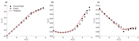
Figure 16.
Aerodynamic force modelling results for NASA CRM-WBT model (case I): (a) ; (b) ; (c) .
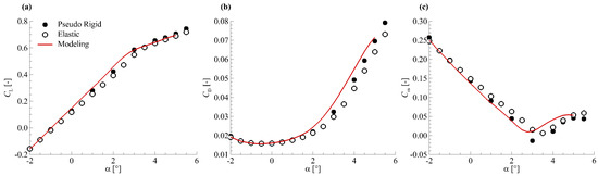
Figure 17.
Aerodynamic force modelling results for NASA CRM-WBT model (case II): (a) ; (b) ; (c) .
For both cases in Figure 16 and Figure 17, it shows: (a) the predicted by the modelling method agrees well with the ‘Pseudo Rigid’ data; the is overestimated by the modelling method compared with the ‘Pseudo Rigid’ result; the predicted by the modelling method is well consistent with the ‘Pseudo Rigid’ data in the linear part of the curve, but there is a great discrepancy between the two results as regards the high angles of attack. Table 4 gives the value of the aerodynamic force coefficients in application case I. The obvious differences between the data of the modelling and ‘Pseudo Rigid’ results in Table 4 indicates that the present modelling method still lacks the ability to accurately predict the aerodynamic force on the rigid model shape for such a complex configuration.
Table 4.
Aerodynamic force coefficients by different methods in application case I.
Since the aerodynamic force modelling is based on some assumptions, it is not a very accurate method compared with other correction methods. The present correction method can only predict a reasonable rather than a very accurate result on complex wind tunnel model shape, which has been demonstrated in Figure 16 and Figure 17 and Table 4. However, as a result of its high efficiency and low cost, the present correction method can be used for quick analysis on the influence of wing deformation in wind tunnel tests. The quick analysis is meaningful to making decision whether to start a more accurate correction on the experimental data. Besides, the quick analysis can also provides aerodynamic forces on rigid shape for comparison.
5. Conclusions
This paper presented a fast correction method to obtain aerodynamic force coefficients by establishing the mathematical modelling between aerodynamic forces and wing section torsion through the radial basis function interpolation. The parametric analysis of the aerodynamic force modelling method is investigated and the test results show that: (1) Wendland’s C6 function with a support radius of 1.0 has a better prediction accuracy of the aerodynamic forces on rigid model shape; (2) deformation perturbation has an obvious influence on aerodynamic force modelling but this influence can be reduced effectively by smoothing the deformation data. Furthermore, the present fast correction method can be applied to predict the aerodynamic forces of a general model, the CRM wing/body/tail configuration. The comparison between prediction and corrected test data demonstrates that the present method can obtain reasonable aerodynamic forces on rigid model shape. However, there is still much space to improve the prediction accuracy on a complex model shape.
Author Contributions
Conceptualization, Y.S. and Y.W.; methodology, Y.S. and Y.W.; software, D.M.; validation, Y.S. and D.M.; formal analysis, Y.S. and A.D.R.; writing—original draft preparation, Y.S.; writing—review and editing, A.D.R.; visualization, Y.S.; supervision, Y.W.; funding acquisition, Y.W. and Y.S.
Funding
This research was funded by National Key R&D Program of China grant number 2016YFB0200703.
Acknowledgments
The first author would like to show his grateful thanks to China Scholarship Council for offering a Talent Training Project grant number 201600930081. With the sponsorship from China Scholarship Council, the first author can visit the University of Southampton and finish this research.
Conflicts of Interest
The authors declare no conflict of interest.
References
- Liu, Y.; Elham, A.; Horst, P.; Hepperle, M. Exploring vehicle level benefits of revolutionary technology progress via aircraft design and optimization. Energies 2018, 11, 166. [Google Scholar] [CrossRef]
- Pallek, D.; Butefisch, K.; Quest, J.; Strudthoff, W. Model deformation measurement in ETW using the moiré technique. In Proceedings of the 20th International Congress on Instrumentation in Aerospace Simulation Facilities (ICIASF’03), Gottingen, Germany, 25–29 August 2003; pp. 110–114. [Google Scholar]
- Liu, D.; Xu, X.; Li, Q.; Peng, X.; Chen, D. Correction of model deformation effects for a supercritical wing in transonic wind tunnel. Tehnički Vjesnik 2017, 24, 1647–1655. [Google Scholar]
- Hantrais-Gervois, J.L.; Destarac, D. Drag polar invariance with flexibility. J. Aircr. 2015, 52, 997–1001. [Google Scholar] [CrossRef]
- Burner, A.; Goad, W.; Massey, E.; Goad, L.; Goodliff, S.; Bissett, O. Wing deformation measurements of the DLR-F6 transport configuration in the National Transonic Facility. In Proceedings of the 26th AIAA Applied Aerodynamics Conference, Honolulu, HI, USA, 18–21 August 2008; p. 6921. [Google Scholar]
- Keye, S.; Rudnik, R. Aero-Elastic Simulation of DLR’s F6 Transport Aircraft Configuration and Comparison to Experimental Data. In Proceedings of the 47th AIAA Aerospace Sciences Meeting Including the New Horizons Forum and Aerospace Exposition, Orlando, FL, USA, 5–8 January 2009; p. 580. [Google Scholar]
- Owens, L.R.; Wahls, R.A.; Rivers, S.M. Off-design Reynolds number effects for a supersonic transport. J. Aircr. 2005, 42, 1427–1441. [Google Scholar] [CrossRef]
- Al-Saadi, J.A. Effect of Reynolds Number, Boundary-Layer Transition, and Aeroelasticity on Longitudinal Aerodynamic Characteristics of a Subsonic Transport Wing; NASA TP-3655; NASA: Washington, DC, USA, 1997.
- Wahls, R.A.; Gloss, B.B.; Flechner, S.G.; Johnson, W.G., Jr.; Wright, F.; Nelson, C.; Nelson, R.; Elzey, M.; Hergert, D. A High Reynolds Number Investigation of a Commercial Transport Model in the National Transonic Facility; NASA TM-4418; NASA: Washington, DC, USA, 1993.
- Rolston, S.; Elsholz, E. Initial Achievements of the European High Reynolds Number Aerodynamic Research Project “HiReTT”. In Proceedings of the 40th AIAA Aerospace Sciences Meeting & Exhibit, Reno, NV, USA, 14–17 January 2002; p. 421. [Google Scholar]
- Rumsey, C.L.; Slotnick, J.P.; Sclafani, A.J. Overview and Summary of the Third AIAA High Lift Prediction Workshop. In Proceedings of the 2018 AIAA Aerospace Sciences Meeting, Kissimmee, FL, USA, 8–12 January 2018; p. 1258. [Google Scholar]
- Derlaga, J.M.; Morrison, J.H. Statistical Analysis of the Sixth AIAA Drag Prediction Workshop Solutions. J. Aircr. 2018, 55, 1388–1400. [Google Scholar] [CrossRef]
- Roy, C.J.; Rumsey, C.L.; Tinoco, E.N. Summary Data from the Sixth AIAA Computational Fluid Dynamics Drag Prediction Workshop: Code Verification. J. Aircr. 2018, 55, 1338–1351. [Google Scholar] [CrossRef]
- Vassberg, J.C.; Tinoco, E.N.; Mani, M.; Rider, B.; Zickuhr, T.; Levy, D.W.; Brodersen, O.P.; Eisfeld, B.; Crippa, S.; Wahls, R.A.; et al. Summary of the fourth AIAA computational fluid dynamics drag prediction workshop. J. Aircr. 2014, 51, 1070–1089. [Google Scholar] [CrossRef]
- Levy, D.W.; Laflin, K.R.; Tinoco, E.N.; Vassberg, J.C.; Mani, M.; Rider, B.; Rumsey, C.L.; Wahls, R.A.; Morrison, J.H.; Brodersen, O.P.; et al. Summary of data from the fifth computational fluid dynamics drag prediction workshop. J. Aircr. 2014, 51, 1194–1213. [Google Scholar] [CrossRef]
- Rivers, M.; Hunter, C.; Campbell, R. Further investigation of the support system effects and wing twist on the NASA common research model. In Proceedings of the 30th AIAA Applied Aerodynamics Conference, New Orleans, LA, USA, 25–28 June 2012; p. 3209. [Google Scholar]
- Hue, D. Fifth drag prediction workshop: ONERA investigations with experimental wing twist and laminarity. J. Aircr. 2014, 51, 1311–1322. [Google Scholar] [CrossRef]
- Tinoco, E.N.; Brodersen, O.; Keye, S.; Laflin, K. Summary of Data from the Sixth AIAA CFD Drag Prediction Workshop: CRM Cases 2 to 5. In Proceedings of the 55th AIAA Aerospace Sciences Meeting, Grapevine, TX, USA, 9–13 January 2017; p. 1208. [Google Scholar]
- Keye, S.; Mavriplis, D. Summary of Case 5 from Sixth Drag Prediction Workshop: Coupled Aerostructural Simulation. J. Aircr. 2017, 55, 1380–1387. [Google Scholar] [CrossRef]
- Ballmann, J. Experimental Analysis of high Reynolds Number structural Dynamics in ETW. In Proceedings of the 46th AIAA Aerospace Sciences Meeting and Exhibit, Reno, NV, USA, 7–10 January 2008; p. 841. [Google Scholar]
- Ballmann, J.; Boucke, A.; Chen, B.; Reimer, L.; Reimer, L.; Behr, M.; Behr, M.; Dafnis, A.; Buxel, C.; Buesing, S.; et al. Aero-structural wind tunnel experiments with elastic wing models at high Reynolds numbers (HIRENASD-ASDMAD). In Proceedings of the 49th AIAA Aerospace Sciences Meeting Including the New Horizons Forum and Aerospace Exposition, Orlando, FL, USA, 4–7 January 2011; p. 882. [Google Scholar]
- Vrchota, P.; Prachař, A. Using wing model deformation for improvement of CFD results of ESWIRP project. CEAS Aeronaut. J. 2018, 9, 361–372. [Google Scholar] [CrossRef]
- Green, J.; Quest, J. A short history of the European Transonic Wind Tunnel ETW. Prog. Aerosp. Sci. 2011, 47, 319–368. [Google Scholar] [CrossRef]
- Edwards, J.W. National transonic facility model and tunnel vibrations. J. Aircr. 2009, 46, 46–52. [Google Scholar] [CrossRef]
- Keye, S.; Brodersen, O. Investigations of Fluid-Structure Coupling and Turbulence Model Effects on the DLR Results of the Fifth AIAA CFD Drag Prediction Workshop. In Proceedings of the 31st AIAA Applied Aerodynamics Conference, San Diego, CA, USA, 24–27 June 2013; p. 2509. [Google Scholar]
- Yasue, K.; Sawada, K. Effect of model deformation on aerodynamic coefficients for the AGARD-B wind tunnel model. Trans. Jpn. Soc. Aeronaut. Space Sci. 2011, 54, 163–172. [Google Scholar] [CrossRef]
- Yasue, K.; Sawada, K. CFD-Aided Evaluation of Reynolds Number Scaling Effect Accounting for Static Model Deformation. Trans. Jpn. Soc. Aeronaut. Space Sci. 2012, 55, 321–331. [Google Scholar] [CrossRef]
- Boutet, J.; Dimitriadis, G. Unsteady Lifting Line Theory Using the Wagner Function for the Aerodynamic and Aeroelastic modelling of 3D Wings. Aerospace 2018, 5, 92. [Google Scholar] [CrossRef]
- Silva, W.A. AEROM: NASA’s Unsteady Aerodynamic and Aeroelastic Reduced-Order modelling Software. Aerospace 2018, 5, 41. [Google Scholar] [CrossRef]
- Kroll, N.; Heinrich, R.; Krueger, W.; Nagel, B. Fluid-structure coupling for aerodynamic analysis and design: A DLR perspective. In Proceedings of the 46th AIAA Aerospace Sciences Meeting and Exhibit, Reno, NV, USA, 7–10 January 2008; p. 561. [Google Scholar]
- Liu, T.; Burner, A.W.; Jones, T.W.; Barrows, D.A. Photogrammetric techniques for aerospace applications. Prog. Aerosp. Sci. 2012, 54, 1–58. [Google Scholar] [CrossRef]
- Burner, A.W. Model Deformation Measurements at NASA Langley Research Center. In Proceedings of the 81st Fluid Dynamics Panel Symposium on Advanced Aerodynamics Measurement Technology, Seattle, WA, USA, 22–25 September 1997; pp. 1–9. [Google Scholar]
- Buhmann, M.D. Radial basis functions. Acta Numer. 2000, 9, 1–38. [Google Scholar] [CrossRef]
- Rendall, T.C.; Allen, C.B. Efficient mesh motion using radial basis functions with data reduction algorithms. J. Comput. Phys. 2009, 228, 6231–6249. [Google Scholar] [CrossRef]
- Buhmann, M.D. Radial Basis Functions: Theory and Implementations; Cambridge University Press: Cambridge, UK, 2003; Volume 12. [Google Scholar]
- Heeg, J. Overview and lessons learned from the aeroelastic prediction workshop. In Proceedings of the 54th AIAA/ASME/ASCE/AHS/ASC Structures, Structural Dynamics, and Materials Conference, Boston, MA, USA, 8–11 April 2013; p. 1798. [Google Scholar]
- Hassan, D.; Ritter, M. Assessment of the ONERA/DLR Numerical Aeroelastics Prediction Capabilities on the HIRENASD Configuration. In Proceedings of the International Forum on Aeroelasticity and Structural Dynamics, Paris, France, 26–30 June 2011. [Google Scholar]
- Menter, F.R. Two-equation eddy-viscosity turbulence models for engineering applications. AIAA J. 1994, 32, 1598–1605. [Google Scholar] [CrossRef]
- Chen, R.; Wang, Z. Fast, block lower-upper symmetric Gauss-Seidel scheme for arbitrary grids. AIAA J. 2000, 38, 2238–2245. [Google Scholar] [CrossRef]
- Reimer, L.; Braun, C.; Chen, B.H.; Ballmann, J. Computational Aeroelastic Design and Analysis of the HIRENASD Wind Tunnel Wing Model and Tests. In Proceedings of the International Forum on Aeroelasticity and Structural Dynamics (IFASD), Stockholm, Sweden, 18–21 June 2007; pp. 17–20. [Google Scholar]
- Vassberg, J.; Dehaan, M.; Rivers, M.; Wahls, R. Development of a common research model for applied CFD validation studies. In Proceedings of the 26th AIAA Applied Aerodynamics Conference, Honolulu, HI, USA, 18–21 August 2008; p. 6919. [Google Scholar]
- Melissa, R. NASA Common Research Model. 2017. Available online: https://commonresearchmodel.larc.nasa.gov/ (accessed on 12 October 2018).
- Rivers, M.B.; Dittberner, A. Experimental investigations of the NASA common research model. J. Aircr. 2014, 51, 1183–1193. [Google Scholar] [CrossRef]
- Rivers, M.; Dittberner, A. Experimental investigations of the nasa common research model in the nasa langley national transonic facility and nasa ames 11-ft transonic wind tunnel. In Proceedings of the 49th AIAA Aerospace Sciences Meeting Including the New Horizons Forum and Aerospace Exposition, Orlando, FL, USA, 4–7 January 2011; p. 1126. [Google Scholar]
- Rivers, M.; Quest, J.; Rudnik, R. Comparison of the NASA Common Research Model European Transonic Wind Tunnel test data to NASA National Transonic Facility test data. CEAS Aeronaut. J. 2018, 9, 307–317. [Google Scholar] [CrossRef]
- Koga, S.; Kohzai, M.; Ueno, M.; Nakakita, K.; Sudani, N. Analysis of NASA Common Research Model Dynamic Data in JAXA Wind Tunnel Tests. In Proceedings of the 51st AIAA Aerospace Sciences Meeting Including the New Horizons Forum and Aerospace Exposition, Grapevine, TX, USA, 7–10 January 2013; p. 495. [Google Scholar]
- Cartieri, A.; Hue, D.; Chanzy, Q.; Atinault, O. Experimental Investigations on the Common Research Model at ONERA-S1MA-Comparison with DPW Numerical Results. In Proceedings of the 55th AIAA Aerospace Sciences Meeting, Grapevine, TX, USA, 9–13 January 2017; p. 0964. [Google Scholar]
- The ESWIRP ETW TNA Test Results. 2014. Available online: http://www.eswirp.eu/ETW-TNA-Dissemination.html (accessed on 12 October 2018).
© 2018 by the authors. Licensee MDPI, Basel, Switzerland. This article is an open access article distributed under the terms and conditions of the Creative Commons Attribution (CC BY) license (http://creativecommons.org/licenses/by/4.0/).