Unsteady Lifting Line Theory Using the Wagner Function for the Aerodynamic and Aeroelastic Modeling of 3D Wings

Abstract

A method is presented to model the incompressible, attached, unsteady lift and pitching moment acting on a thin three-dimensional wing in the time domain. The model is based on the combination of Wagner theory and lifting line theory through the unsteady Kutta–Joukowski theorem. The results are a set of closed-form linear ordinary differential equations that can be solved analytically or using a Runge–Kutta–Fehlberg algorithm. The method is validated against numerical predictions from an unsteady vortex lattice method for rectangular and tapered wings undergoing step or oscillatory changes in plunge or pitch. Further validation is demonstrated on an aeroelastic test case of a rigid rectangular finite wing with pitch and plunge degrees of freedom.

1. Introduction

Closed-form solutions for the attached incompressible unsteady flow problem around a two-Dimensional (2D) airfoil exist in both the frequency domain [1] and in the time domain:

• Wagner theory [2,3]
• Finite state flow model [4]
• Leishman unsteady state space representation [5]

For three-Dimensional (3D) wings, there exists one closed-form solution for the unsteady aerodynamics of elliptical wings [2]. For general geometries, closed-form solutions are usually obtained either from strip theory (see for example Dowell [6]) or from panel methods, such as the Doublet Lattice Method (DLM) [7] or the Vortex Lattice Method (VLM) [8]. Strip theory is based on estimating the 3D unsteady loads by integrating 2D loads along the span. It therefore ignores the downwash induced by the trailing vortices and overestimates the lift; it is mostly used on lifting surfaces with very high aspect ratios, such as helicopter or wind turbine blades. The DLM can be used to estimate modal, frequency domain aerodynamic loads in the form of the generalized aerodynamic force matrix. This matrix is evaluated numerically at discrete reduced frequency values and is interpolated in order to estimate the aerodynamic loads at intermediate frequencies. The generalized force matrix can be transformed to the time domain using the rational function, the Chebyshev polynomial or indicial function representations, again based on a set of discrete frequency estimations. Several efficient transformation methodologies have been developed, notably the minimum state approach [9], but they remain approximations. The Vortex Lattice Method can also be used to derive a generalized aerodynamic force matrix [10,11], which can then be transformed to the time domain.

Alternative closed-form solutions of the 3D attached flow problem include Reissner’s method [12], which combined the Theodorsen and lifting line theories and was formulated in the frequency domain. Chopra [13] developed expressions for the lift, thrust and moment of lunate tails oscillating in pitch and plunge, based on the lifting line assumption that the flow is locally 2D around cross-sections of the wing’s span, but that the local angle of attack is influenced by the vorticity in the wake. The work was limited to rectangular wings, and frequency domain solutions for the aerodynamic loads were obtained. Furthermore, Chopra and Kambe [14] formulated an unsteady lifting surface theory and applied it to wings with non-rectangular planforms, but the aerodynamic load calculations were still calculated in the frequency domain. James [15] developed an unsteady lifting line theory for wings of a large aspect ratio with smooth tip geometries (such as elliptical planforms). He used a matched asymptotic expansion approach to obtain solutions for impulsively-started motion, constant acceleration and sinusoidal oscillations in pitch, plunge or flap. Nevertheless, the method failed to yield total aerodynamic loads for wings with chords that jump abruptly to zero at the tip (such as rectangular or trapezoidal wings). Furthermore, Ahmadi and Widnall [16] argued that James’s theory is only valid for low reduced frequencies and that its 3D results are incorrect. Van Holten [17] also used a matched asymptotic expansion to develop an unsteady lifting line theory for pitching wings and rotating blades, but Ahmadi and Widnall [16] again claimed that the work is only valid for low reduced frequencies. Phlips et al. [18] derived a time domain unsteady lifting line theory for flapping (but not pitching) wings.

Other frequency domain unsteady lifting line approaches were proposed by Dragos [19], Sclavounos [20] and, more recently, Drela [21]. State-space time domain models are usually quasi-steady, such as the models by Nabawy and Crowther [22,23]. The present paper details a robust, closed-form, time domain, 3D unsteady aerodynamic model that does not involve a transformation from the frequency domain. The approach is based on Wagner’s 2D unsteady lift theory and Prandtl’s lifting line theory and will be referred to as the Wagner Lifting Line (WLL) method. It was first proposed by Boutet and Dimitriadis [24], but is presented here in much more detail, including an aeroelastic extension. A similar approach was proposed slightly later by Izraelevitz et al. [25], but this technique was not extended to aeroelastic applications.

2. Method

As mentioned in the Introduction, one of the main characteristics of lifting line theories is that the flow is two-dimensional around spanwise cross-sections, but the local angle of attack is affected by the downwash induced by the wake. In the classical version of the theory, the wing and wake are modeled using a superposition of horseshoe vortices, the strength of which is constant in time. In this way, the wake is straight and semi-infinite, and its strength varies in the spanwise, but not in the chordwise direction.

In Wagner’s and Theodorsen’s 2D unsteady aerodynamic theories, the wake is still straight and semi-infinite, but its strength varies in the chordwise direction since it is calculated from the unsteady Kutta condition. The wake is assumed to propagate with the free stream velocity, U, so that chordwise displacement and time are directly related by the equation $x=Ut$. A change in vorticity at the trailing edge that occurs at time $t_0$ will be reflected in the wake at a downstream distance $U(t-t_0)$ at time t.

Lifting line and Wagner theories are not directly compatible because in the former, the chordwise strength of the trailing vortices is constant, while in the latter, it varies. In the present work, Wagner theory is applied to spanwise cross-sections, so that the strength of the wake varies in both the spanwise and chordwise direction. A quasi-steady version of lifting line theory is used in order to approximate the downwash velocity caused by the wake and to add it to the other sources of downwash used in Wagner theory.

There are three sources of downwash on finite wings in unsteady flow:

• Geometric downwash due to camber and twist.
• Downwash due to the motion of the wing (including the free stream and angle of attack).
• Downwash due to the three-dimensionality of the flow (wing tip vortex effect).

The 3D downwash will be calculated using Prandtl’s lifting line theory, as detailed in Kuethe and Chow [26]. The other two downwash contributions will be modeled from Wagner’s unsteady aerodynamic theory, as presented by Fung [3].

2.1. Lifting Line Theory

A truncated Fourier series is used to represent an arbitrary time-varying circulation distribution along the span of a flat plate wing:

$$\begin{array}{ccc}\hfill \Gamma (t,y)& =& \frac{1}{2}{a}_0{c}_{0}U\sum _{n=1}^m{a}_n(t)sin(n\theta )\hfill \end{array}$$

(1)

where $a_0$ is the lift curve slope at the wing’s axis of symmetry, $c_0$ is the chord length at the wing’s axis of symmetry, U is the free stream airspeed, $a_n(t)$ are the time varying Fourier coefficients, m is the number of terms kept in the series, $\theta$ comes from the substitution $y=(s/2)cos(\theta )$, y represents the location along the span and s represents the span of the wing. In the classical lifting line theory, the wing is split into m spanwise strips, and the order of the Fourier series is also m, so that the number of unknowns (Fourier coefficients $a_n$) is equal to the number of equations (spanwise strips). Izraelevitz et al. [25] proposed an alternative approach, whereby a horseshoe vortex representation was used to model the 3D wing circulation.

Using Prandtl’s lifting line theory, it is possible to compute the downwash $w_y$ caused by the 3D circulation distribution at a location y along the wing span:

$$\begin{array}{ccc}\hfill w_y& =& -\frac{1}{4\pi }{\int }_{-s/2}^{s/2}\frac{\mathrm{d}\Gamma /\mathrm{d}{y}_0}{y-y_0}\mathrm{d}{y}_0\hfill \\ & =& -\frac{a_0{c}_{0}U}{4\pi s}\sum _{n=1}^{m}n{a}_n(t){\int }_0^{\pi }\frac{cos(n{\theta }_0)}{cos({\theta }_0)-cos(\theta )}\mathrm{d}{\theta }_0\hfill \end{array}$$

(2)

Glauert [27] evaluated the integral in this latest expression, so that the downwash $w_y$ can be computed as a function of the Fourier coefficients and the location $y(\theta )$ along the span:

$$\begin{array}{ccc}\hfill w_y(t)& =& -\frac{a_0{c}_{0}U}{4s}\sum _{n=1}^{m}n{a}_n(t)\frac{sin(n\theta )}{sin\theta }\hfill \end{array}$$

(3)

Note that this is a quasi-steady version of lifting line theory, since any instantaneous changes in vorticity over the wing affect the entire wake simultaneously.

2.2. Unsteady Kutta–Joukowski

It is possible to express the unsteady sectional lift coefficient as a function of $a_n(t)$ and location along the span y, using the unsteady Kutta–Joukowski theorem and considering a lumped spanwise vortex element, as explained by Katz and Plotkin [8] on page 439. The circulatory sectional lift coefficient becomes:

$$\begin{array}{ccc}\hfill c_l^c(t,y)& =& \frac{2\Gamma }{Uc(y)}+\frac{2\dot{\Gamma }}{U^2}\hfill \end{array}$$

(4)

where $\Gamma$ is the vortex strength, $c(y)$ is the chord at span section y and the unsteady term $\dot{\Gamma }$ comes from the unsteady Bernoulli equation. The vortex strength can be replaced by its Fourier series representation from Equation (1), to obtain:

$$\begin{array}{ccc}\hfill c_l^c(t,y)& =& a_0\sum _{n=1}^m\left(\frac{c_0}{c}{a}_n+\frac{c_0}{U}{\dot{a}}_n\right)sin(n\theta )\hfill \end{array}$$

(5)

Furthermore, the circulatory lift coefficient for the entire wing can be computed from:

$$\begin{array}{ccc}\hfill C_l^c(t)& =& {\int }_{-s/2}^{s/2}\frac{\frac{1}{2}\rho U^{2}c(y)c_l^c(t,y)\mathrm{d}y}{\frac{1}{2}\rho U^{2}S}\hfill \end{array}$$

(6)

where S is the wing’s surface area.

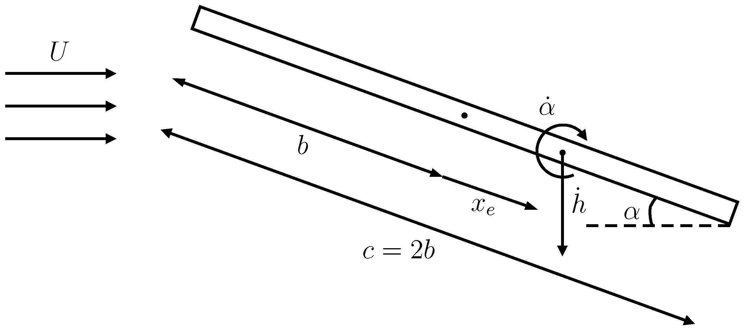
The lift will cause a pitching moment around the pitch axis of each wing section, i.e., the axis around which the wing section can pitch. One can compute the circulatory moment distribution from the lift distribution, assuming that the sectional lift acts on the quarter chord. Refer to Figure 1, which shows a wing section with chord c and half-chord b at pitch angle $\alpha$ to a free stream U. The position of the pitch axis, $x_e$, is defined with respect to the half-chord point. The circulatory sectional moment equation is simply:

$$\begin{array}{c}\hfill c_m^c(t,y)=\frac{c(y)/4+x_e(y)}{c(y)}{c}_l^c(t,y)\end{array}$$

(7)

where $x_e$ and c are allowed to vary in the spanwise direction y. Note that the pitch axis is measured from the mid-chord point and is defined as positive if it lies downstream of that point as chosen by Theodorsen [1]. The total circulatory moment coefficient is:

$$\begin{array}{ccc}\hfill C_m^c(t)& =& {\int }_{-s/2}^{s/2}\frac{\frac{1}{2}\rho U^{2}c{(y)}^2{c}_m^c(t,y)\mathrm{d}y}{\frac{1}{2}\rho U^{2}S\overline{c}}\hfill \end{array}$$

(8)

where $\overline{c}=S/s$ is the mean chord.

2.3. Wagner’s Sectional Circulatory Lift

The computation of the unsteady circulatory aerodynamic loads is based on the circulatory sectional lift $c_l^c(t,y)$ response of an airfoil undergoing a step change in downwash $\Delta w(y)<<U$ at span location y. The resulting step change in the lift coefficient can be expressed in terms of the Wagner function, $\mathsf{\Phi }(t)$, as follows:

$$\begin{array}{ccc}\hfill c_l^c(t,y)& =& a_0(y)\mathsf{\Phi }(t)\frac{\Delta w(y)}{U}\hfill \end{array}$$

(9)

where $a_0(y)$ is the lift curve slope of the local airfoil section, which is approximated by $2\pi$ for thin airfoils, and $\mathsf{\Phi }(t)$ is Jones’ [28] approximation of the Wagner function:

$$\begin{array}{ccc}\hfill \mathsf{\Phi }(t)& =& 1-{\mathsf{\Psi }}_1{e}^{-\frac{{ϵ}_{1}U}{b}t}-{\mathsf{\Psi }}_2{e}^{-\frac{{ϵ}_{2}U}{b}t}\hfill \end{array}$$

with ${\mathsf{\Psi }}_1=0.165$, ${\mathsf{\Psi }}_2=0.335$, ${ϵ}_1=0.0455$ and ${ϵ}_2=0.3$.

Duhamel’s principle can be applied to Equation (9) in order to express a continuous lift response as the time integral of infinitesimal step responses:

$$\begin{array}{ccc}\hfill c_l^c(t,y)& =& a_0(y)\left(\frac{w(0,y)}{U}\mathsf{\Phi }(t)+{\int }_0^t\frac{1}{U}\frac{\partial w(\tau ,y)}{\partial \tau }\mathsf{\Phi }(t-\tau )\mathrm{d}\tau \right)\hfill \end{array}$$

(10)

The troublesome $\frac{\partial w(\tau ,y)}{\partial \tau }$ term inside the integral can be removed by applying integration by parts, such that:

$$\begin{array}{ccc}\hfill c_l^c(t,y)& =& a_0(y)\left(\frac{w(t,y)}{U}\mathsf{\Phi }(0)-{\int }_0^t\frac{1}{U}\frac{\partial \mathsf{\Phi }(t-\tau )}{\partial \tau }w(\tau ,y)\mathrm{d}\tau \right)\hfill \end{array}$$

(11)

The downwash $w(t,y)$ must now be computed; it will depend on the kinematics of the wing. In this work, the wing is assumed to be rigid with pitch and plunge degrees of freedom, but flexible wings with bending and torsion modes can also be considered. Figure 1 defines the local plunge and pitch degrees of freedom, $h(t,y)$ and $\alpha (t,y)$, respectively. A local downwash $w_y$ is added in order to represent the 3D downwash effects, so that $w(t,y)$ becomes:

$$\begin{array}{ccc}\hfill w(t,y)& =& U\alpha (t,y)+\dot{h}(t,y)+\dot{\alpha }(t,y)d+w_y(t)\hfill \\ \hfill d& =& \left(\frac{1}{2}-a\right)b\hfill \\ \hfill a& =& \frac{x_e}{b}\hfill \end{array}$$

(12)

where d is the non-dimensional distance between the mid-chord and the pitch axis, as defined by Theodorsen [1]. After combining Equations (11) and (12),

$$\begin{array}{ccc}\hfill \frac{c_l^c(t,y)}{a_0(y)}& =& \left(\alpha +\frac{\dot{h}}{U}+\frac{\dot{\alpha }d}{U}+\frac{w_y}{U}\right)\mathsf{\Phi }(0)\hfill \\ & +& {\int }_0^t{\mathsf{\Psi }}_1{ϵ}_1\frac{U}{b}{e}^{\frac{-{ϵ}_{1}U}{b}(t-\tau )}\left(\alpha (\tau )+\frac{\dot{h}(\tau )}{U}+\frac{\dot{\alpha }(\tau )d}{U}+\frac{w_y(\tau )}{U}\right)\mathrm{d}\tau \hfill \\ & +& {\int }_0^t{\mathsf{\Psi }}_2{ϵ}_2\frac{U}{b}{e}^{\frac{-{ϵ}_{2}U}{b}(t-\tau )}\left(\alpha (\tau )+\frac{\dot{h}(\tau )}{U}+\frac{\dot{\alpha }(\tau )d}{U}+\frac{w_y(\tau )}{U}\right)\mathrm{d}\tau \hfill \end{array}$$

(13)

The following changes of variables are performed in order to eliminate the integrals from Equation (13), where the variables $z_k(t)$ are called aerodynamics states.

$$\begin{array}{cccc}\hfill z_1(t,y)& ={\int }_0^t{e}^{\frac{-{ϵ}_{1}U}{b}(t-\tau )}h(\tau ,y)\mathrm{d}\tau \hfill & \hfill z_4(t,y)& ={\int }_0^t{e}^{\frac{-{ϵ}_{2}U}{b}(t-\tau )}\alpha (\tau ,y)\mathrm{d}\tau \hfill \\ \hfill z_2(t,y)& ={\int }_0^t{e}^{\frac{-{ϵ}_{2}U}{b}(t-\tau )}h(\tau ,y)\mathrm{d}\tau \hfill & \hfill z_5(t,y)& ={\int }_0^t{e}^{\frac{-{ϵ}_{1}U}{b}(t-\tau )}\frac{w_y(\tau )}{U}\mathrm{d}\tau \hfill \\ \hfill z_3(t,y)& ={\int }_0^t{e}^{\frac{-{ϵ}_{1}U}{b}(t-\tau )}\alpha (\tau ,y)\mathrm{d}\tau \hfill & \hfill z_6(t,y)& ={\int }_0^t{e}^{\frac{-{ϵ}_{2}U}{b}(t-\tau )}\frac{w_y(\tau )}{U}\mathrm{d}\tau \hfill \end{array}$$

(14)

Working through the integrals, we obtain:

$$\begin{array}{ccc}\hfill \frac{c_l^c(t,y)}{a_0(y)}& =& \left(\alpha +\frac{\dot{h}}{U}+\frac{\dot{\alpha }d}{U}+\frac{w_y}{U}\right)\mathsf{\Phi }(0)-\dot{\mathsf{\Phi }}(t)\left(\frac{h(0)}{U}+\frac{\alpha (0)d}{U}\right)\hfill \\ & +& \dot{\mathsf{\Phi }}(0)\left(\frac{h}{U}+\frac{\alpha d}{U}\right)-{\mathsf{\Psi }}_1{ϵ}_1^2\frac{U}{b^2}{z}_1-{\mathsf{\Psi }}_2{ϵ}_2^2\frac{U}{b^2}{z}_2\hfill \\ & +& {\mathsf{\Psi }}_1{ϵ}_1\frac{U}{b}\left(1-\frac{{ϵ}_{1}d}{b}\right)z_3+{\mathsf{\Psi }}_2{ϵ}_2\frac{U}{b}\left(1-\frac{{ϵ}_{2}d}{b}\right)z_4+{\mathsf{\Psi }}_1{ϵ}_1\frac{U}{b}{z}_5+{\mathsf{\Psi }}_2{ϵ}_2\frac{U}{b}{z}_6\hfill \end{array}$$

(15)

First order differential equations for the aerodynamic state variables can be derived using Leibniz’s integral rule. As an example, the equation for $z_1(t,y)$ is:

$$\begin{array}{ccc}\hfill \dot{z_1}(t,y)& =& e^{\frac{-{ϵ}_{1}U(t-t)}{b}}h(t,y)\frac{\partial t}{\partial t}-e^{\frac{-{ϵ}_{1}U\tau }{b}}h(0,y)\frac{\partial 0}{\partial t}-\frac{{ϵ}_{1}U}{b}{\int }_0^t{e}^{\frac{-{ϵ}_{1}U}{b}(t-\tau )}h(\tau ,y)\mathrm{d}\tau \hfill \\ & =& h-\frac{{ϵ}_{1}U}{b}{z}_1(t,y)\hfill \end{array}$$

(16)

The equations for all the aerodynamic states are given by:

$$\begin{array}{cccc}\hfill \dot{z_1}(t,y)& =h-\frac{{ϵ}_{1}U}{b}{z}_1(t,y)\hfill & \hfill \dot{z_4}(t,y)& =\alpha -\frac{{ϵ}_{2}U}{b}{z}_4(t,y)\hfill \\ \hfill \dot{z_2}(t,y)& =h-\frac{{ϵ}_{2}U}{b}{z}_2(t,y)\hfill & \hfill \dot{z_5}(t,y)& =\frac{w_y}{U}-\frac{{ϵ}_{1}U}{b}{z}_5(t,y)\hfill \\ \hfill \dot{z_3}(t,y)& =\alpha -\frac{{ϵ}_{1}U}{b}{z}_3(t,y)\hfill & \hfill \dot{z_6}(t,y)& =\frac{w_y}{U}-\frac{{ϵ}_{2}U}{b}{z}_6(t,y)\hfill \end{array}$$

(17)

Finally, the continuous unsteady circulatory lift coefficient can be written as follows:

$$\begin{array}{ccc}\hfill c_l^c(t,y)& =& \mathbf{C}\dot{\mathbf{q}}+\mathbf{D}\mathbf{q}+\mathbf{E}\mathbf{z}+r\dot{\mathsf{\Phi }}(t)+a_0(y)\mathsf{\Phi }(0)\frac{w_y}{U}\hfill \end{array}$$

(18)

$$\begin{array}{ccc}\hfill \dot{\mathbf{z}}& =& \mathbf{W}\mathbf{z}+\mathbf{F}\mathbf{q}+\mathbf{G}\frac{w_y}{U}\hfill \end{array}$$

(19)

where:

$$\begin{array}{ccc}\hfill \mathbf{q}& =& {\left[\begin{array}{cc}h(t,y)& \alpha (t,y)\end{array}\right]}^T\hfill \\ \hfill \mathbf{z}& =& {\left[\begin{array}{cccccc}{z}_1(t,y)& z_2(t,y)& z_3(t,y)& z_4(t,y)& z_5(t,y)& z_6(t,y)\end{array}\right]}^T\hfill \\ \hfill \mathbf{D}& =& \frac{a_0(y)}{U}\left[\begin{array}{cc}\dot{\mathsf{\Phi }}(0)& U\mathsf{\Phi }(0)+d\dot{\mathsf{\Phi }}(0)\end{array}\right]\hfill \\ \hfill \mathbf{E}& =& \frac{a_0(y)U}{b}\left[\begin{array}{cccccc}-\frac{{\mathsf{\Psi }}_1{ϵ}_1^2}{b}& -\frac{{\mathsf{\Psi }}_2{ϵ}_2^2}{b}& {\mathsf{\Psi }}_1{ϵ}_1\left(1-{ϵ}_1\frac{d}{b}\right)& {\mathsf{\Psi }}_2{ϵ}_2\left(1-{ϵ}_2\frac{d}{b}\right)& {\mathsf{\Psi }}_1{ϵ}_1& {\mathsf{\Psi }}_2{ϵ}_2\end{array}\right]\hfill \\ \hfill \mathbf{G}& =& {\left[\begin{array}{cccccc}0& 0& 0& 0& 1& 1\end{array}\right]}^T\hfill \\ \hfill \mathbf{C}& =& \frac{a_0(y)}{U}\mathsf{\Phi }(0)\left[\begin{array}{cc}1& d\end{array}\right]\hfill \\ \hfill r& =& -\frac{a_0(y)}{U}\left(h(0,y)+d\alpha (0,y)\right)\hfill \\ \hfill \mathbf{W}& =& -\frac{U}{b}\mathrm{diag}\left({ϵ}_1,{ϵ}_2,{ϵ}_1,{ϵ}_2,{ϵ}_1,{ϵ}_2\right)\hfill \\ \hfill \mathbf{F}& =& {\left[\begin{array}{cccccc}1& 1& 0& 0& 0& 0\\ 0& 0& 1& 1& 0& 0\end{array}\right]}^T\hfill \end{array}$$

2.4. Added Mass Effect

The non-circulatory sectional lift and moment coefficients, also known as the added mass effect, can be computed from the non-circulatory terms derived by Theodorsen [1]:

$$\begin{array}{ccc}\hfill c_l^i(t,y)& =& \frac{\pi b}{U^2}\left(\ddot{h}-ab\ddot{\alpha }\right)+\frac{\pi b}{U}\dot{\alpha }\hfill \end{array}$$

(20)

$$\begin{array}{ccc}\hfill c_m^i(t,y)& =& \frac{\pi b}{2U^2}\left[a\ddot{h}-\left(a^2+\frac{1}{8}\right)b\ddot{\alpha }\right]-\left(\frac{1}{2}-a\right)\frac{\pi b}{2U}\dot{\alpha }\hfill \end{array}$$

(21)

The computation of the total non-circulatory lift $C_l^i$ and moment $C_m^i$ coefficients follows the same principle as Equations (6) and (8), and the final result is given in Equations (A26) and (A27) for a rectangular wing.

2.5. Assembling the Pieces Together

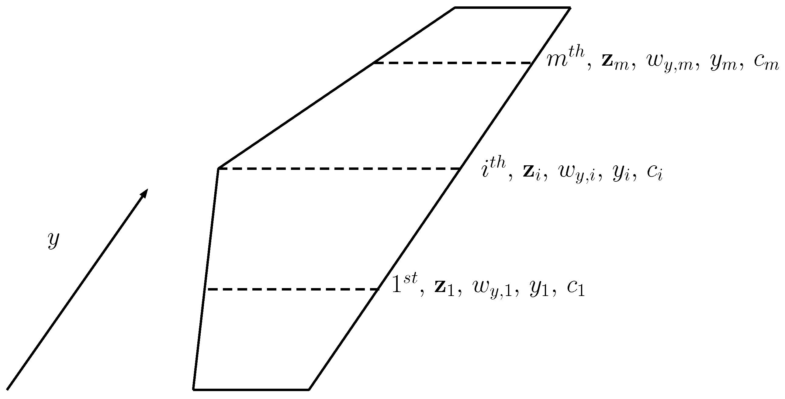
In order to compute the m Fourier coefficients $a_n$, m spanwise wing strips are considered, as shown in Figure 2, which represents m strips along the wing span, their respective local aerodynamics variables ${\mathbf{z}}_{\mathbf{i}}$, 3D downwash effects $w_{y,i}$ and chord section $c_i$. For an arbitrary strip i, Equations (1), (18) and (19) can be combined to obtain the following system:

$$\begin{array}{ccc}\hfill \stackrel{c_l^c(t,y_i)}{\overbrace{a_0(y_i){\sum }_{n=1}^m\left(\frac{c_0}{c_i}{a}_n+\frac{c_0}{U}{\dot{a}}_n\right)sin(n{\theta }_i)}}& =& {\mathbf{C}}_{\mathbf{i}}\dot{\mathbf{q}}+{\mathbf{D}}_{\mathbf{i}}\mathbf{q}+{\mathbf{E}}_{\mathbf{i}}{\mathbf{z}}_i+a_0(y_i)\mathsf{\Phi }(0)\frac{w_{y_i}}{U}\hfill \\ \hfill \dot{{\mathbf{z}}_i}& =& {\mathbf{W}}_{\mathbf{i}}{\mathbf{z}}_i+\mathbf{F}\mathbf{q}+\mathbf{G}\frac{w_{y_i}}{U}\hfill \end{array}$$

(22)

The variables ${\mathbf{z}}_i$ represent the local aerodynamic state variables for the i-th strip. Matrices ${\mathbf{C}}_{\mathbf{i}}$, ${\mathbf{D}}_{\mathbf{i}}$, ${\mathbf{E}}_{\mathbf{i}}$ and ${\mathbf{W}}_{\mathbf{i}}$ are the matrices computed in Section 2.3 where the chord c is replaced with its local value $c_i$. Variable $w_{y_i}$ represents the 3D downwash effect on the i-th strip; its value is given by Equation (3). Substituting for $w_{y_i}$ and re-arranging, Equation (22) become:

$$\begin{array}{ccc}\hfill a_0(y_i)\sum _{n=1}^m\left(\left(\frac{c_0}{c_i}+\mathsf{\Phi }(0)\frac{a_0{c}_{0}n}{4ssin({\theta }_i)}\right)a_n+\frac{c_0}{U}{\dot{a}}_n\right)sin(n{\theta }_i)& =& {\mathbf{C}}_{\mathbf{i}}\dot{\mathbf{q}}+{\mathbf{D}}_{\mathbf{i}}\mathbf{q}+{\mathbf{E}}_{\mathbf{i}}{\mathbf{z}}_i\hfill \end{array}$$

$$\begin{array}{ccc}\hfill \dot{{\mathbf{z}}_i}& =& {\mathbf{W}}_{\mathbf{i}}{\mathbf{z}}_i+\mathbf{F}\mathbf{q}-\mathbf{G}\frac{a_0{c}_0}{4s}\sum _{n=1}^{m}n{a}_n(t)\frac{sin(n{\theta }_i)}{sin{\theta }_i}\hfill \end{array}$$

(23)

Applying Equation (23) to all m strips, a set of $7m$ ordinary linear differential equations for $7m$ unknowns (m for the Fourier coefficients $a_n$ and $6m$ for the aerodynamic states ${\mathbf{z}}_1,\dots {\mathbf{z}}_m$) is obtained. Once this system of ODEs is solved and the coefficients $a_n(t)$ are evaluated, the lift distribution acting on the wing can be computed from Relation (5), the total lift from (6) and the total pitching moment from (8). As an example, the computation of the aerodynamic loads for a rectangular wing is fully detailed in the Appendix, Equations (A1)–(A29).

2.6. Asymptotic Behavior for a Rectangular Wing ($c=c_0$)

By imposing stationarity, all derivatives in time vanish and the system of Equation (23) should reduce to the classical lifting line theory. After imposing stationarity on Equation (17), the aerodynamic states variables become:

$$\begin{array}{cccc}\hfill z_1(y)& =\frac{b}{{ϵ}_{1}U}h(y)\hfill & \hfill z_4(y)& =\frac{b}{{ϵ}_{2}U}\alpha (y)\hfill \\ \hfill z_2(y)& =\frac{b}{{ϵ}_{2}U}h(y)\hfill & \hfill z_5(y)& =\frac{b}{{ϵ}_1{U}^2}{w}_y\hfill \\ \hfill z_3(y)& =\frac{b}{{ϵ}_{1}U}\alpha (y)\hfill & \hfill z_6(y)& =\frac{b}{{ϵ}_2{U}^2}{w}_y\hfill \end{array}$$

(24)

Injecting these expressions in Equation (23) and applying the necessary simplifications, the system becomes:

$$a_0(y)\sum _{n=1}^m\left(1+\mathsf{\Phi }(0)\frac{a_0(y)nc}{4ssin({\theta }_i)}\right)a_{n}sin(n{\theta }_i)=a_0(y)\alpha (y)+a_0(y)\mathsf{\Phi }(0)\frac{w_y}{U}$$

or:

$$\sum _{n=1}^m\left(1+\frac{a_0(y)nc}{4ssin({\theta }_i)}\right)a_{n}sin(n{\theta }_i)=\alpha (y)$$

which is the equation derived by Kuethe and Chow [26] for a rectangular wing, using Prandtl’s lifting line theory for a constant pitch angle $\alpha (y)=\alpha$.

If the span of the wing is infinite, $s=\infty$, all 3D effects vanish and System (23) should reduce to the 2D Wagner solution. Looking at Equation (3), it is obvious that $\underset{s\to \infty }{lim}{w}_y=0$. It can then be shown from Equation (14) that $z_5=0$ and $z_6=0$. The system of Equation (23) is now reduced to:

$$\begin{array}{ccc}\hfill c_l^c(t)& =& a_0(y)\sum _{n=1}^m\left(a_n+\frac{c}{U}{\dot{a}}_n\right)sin(n{\theta }_i)=\mathbf{C}\dot{\mathbf{q}}+\mathbf{D}\mathbf{q}+\mathbf{E}{\mathbf{z}}_i\hfill \\ \hfill \dot{{\mathbf{z}}_i}& =& \mathbf{W}{\mathbf{z}}_i+\mathbf{F}\mathbf{q}\hfill \\ \hfill {\mathbf{z}}_{\mathbf{i}}& =& {\left[\begin{array}{cccccc}{z}_{1,i}& z_{2,i}& z_{3,i}& z_{4,i}& 0& 0\end{array}\right]}^T\hfill \end{array}$$

(25)

which is the classical 2D Wagner formulation, as given by Fung [3] for all arbitrary strips i.

3. Test Cases

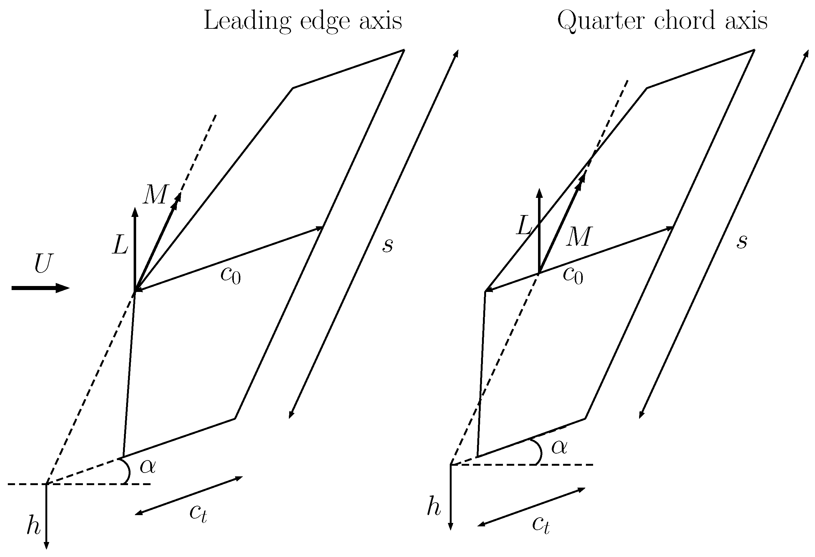
The Wagner lifting line method is applied here to a rectangular and a tapered wing. The rectangular wing, shown in Figure 3, has constant chord $c=1$ m, span s, surface $S=cs$ and aspect ratio $AR=s^2/S$. It has two degrees of freedom, a pure plunge $h(t,y)=h(t)$ and a pure pitch angle $\alpha (t,y)=\alpha (t)$ around its pitch axis. Two positions of the pitch axis are considered: one at the leading edge and one at the quarter chord.

The tapered wing, shown in Figure 4, has root chord $c_0=1$ m, tip chord $c_t=0.5$ m, span s, surface $S=\left(c_0+c_t\right)\frac{s}{2}$ and aspect ratio $AR=s^2/S$. It has the same degrees of freedom as the rectangular wing. The pitch axis is defined with respect to the root chord, as shown in Figure 4. Again, leading edge and quarter chord pitch axis locations are considered.

3.1. Types of Motion

The degrees of freedom of the wings are subjected to two kinds of motion: step changes and sinusoidal oscillations. The step is expressed as the function $f=A\left(1-e^{-10t}\right)$ where t is the time and A is the position of the degree of freedom after the step. Steps $\Delta h=0.1$ m and $\Delta \alpha =5^{\circ }$ are separately applied to the plunge and pitch degrees of freedom.

Sinusoidal oscillations with ten distinct frequencies are tested separately for each degree of freedom, in order to assess the WLL model’s frequency response. The oscillations are expressed as $f=Acos\left(\frac{2Uk}{c_0}t\right)$ where t is the time, A the amplitude of the oscillation and $k=[0.1,0.2,0.3\dots 1]$ is the reduced frequency. The pitch and plunge amplitudes are respectively set to $A=5^{\circ }$ and $A=0.1$ m.

3.2. Validation

The unsteady Vortex Lattice Method (VLM) is used as a reference solution to which the results obtained by the Wagner lifting line approach are to be compared. The particular implementation of the VLM used here is more thoroughly described by Dimitriadis et al. [29]. The difference between the solutions obtained from WLL and VLM is quantified using the Normalized Root-Mean-Square Deviation (NRMSD).

$$\begin{array}{ccc}\hfill RMSD& =& \sqrt{\frac{{\sum }_{t=1}^N{\left(y_{w,r}-y_{v,r}\right)}^2}{N}}\hfill \end{array}$$

(26)

$$\begin{array}{ccc}\hfill NRMSD& =& 100\times \frac{RMSD}{max(y_v)-min(y_v)}[\%]\hfill \end{array}$$

(27)

where N is the number of time instances, $y_{v,r}$ represents the lift or moment coefficient computed by the VLM at the r-th time instance and $y_{w,r}$ represents the lift or moment coefficient computed by the WLL approach at the r-th time instance.

4. Convergence

The differential Equation (23) are solved by means of a Runge–Kutta–Fehlberg fourth and fifth order numerical time integration technique. A time convergence analysis is therefore needed in order to minimize numerical integration errors without increasing the computation time too much. A convergence analysis is also performed for the vortex lattice method.

As shown in Equation (1), the WLL uses a truncated Fourier series with m coefficients, which correspond to the m spanwise strips shown in Figure 2. A spatial convergence study must also be carried out in order to determine the effect of the number of strips on the aerodynamic load predictions. Note that the number of states in the system is $7m$; therefore, keeping m as low as possible is important. The NRMSD is used in order to determine if convergence has been achieved, such that:

$$\begin{array}{ccc}\hfill RMSD(i)& =& \sqrt{\frac{{\sum }_{t=1}^N{\left(y_{i,t}-y_{ref,t}\right)}^2}{N}}\hfill \end{array}$$

(28)

$$\begin{array}{ccc}\hfill NRMSD(i)=e(i)& =& 100\times \frac{RMSD}{max(y_{ref})-min(y_{ref})}[\%]\hfill \end{array}$$

(29)

where $y_{i,t}$ represents the lift coefficient response at the t-th time instance for the i-th value of the convergence parameter. The latter can be either the time step tolerance of the Runge–Kutta–Fehlberg scheme or the number of strips; $y_{ref}$ represents the reference lift coefficient against which the convergence is assessed. This reference is computed for an appropriately high value of the convergence parameter.

4.1. Runge-Kutta Convergence

The time step tolerance controls the error of the Runge-Kutta time integration scheme. Given the solution arrays ${\mathbf{r}}_4$ and ${\mathbf{r}}_5$ of the respective fourth and fifth order Runge-Kutta estimates for a current time $t_i$ and time step $\Delta t$, the Runge–Kutta–Fehlberg algorithm used in this work is given by:

• if $Tol<({\mathbf{r}}_5-{\mathbf{r}}_4){({\mathbf{r}}_5-{\mathbf{r}}_4)}^T$, reduce the time step to $\Delta t/2$
• otherwise, go to the next time instance $t_{i+1}=t_i+\Delta t$ and reset $\Delta t$ to its default value

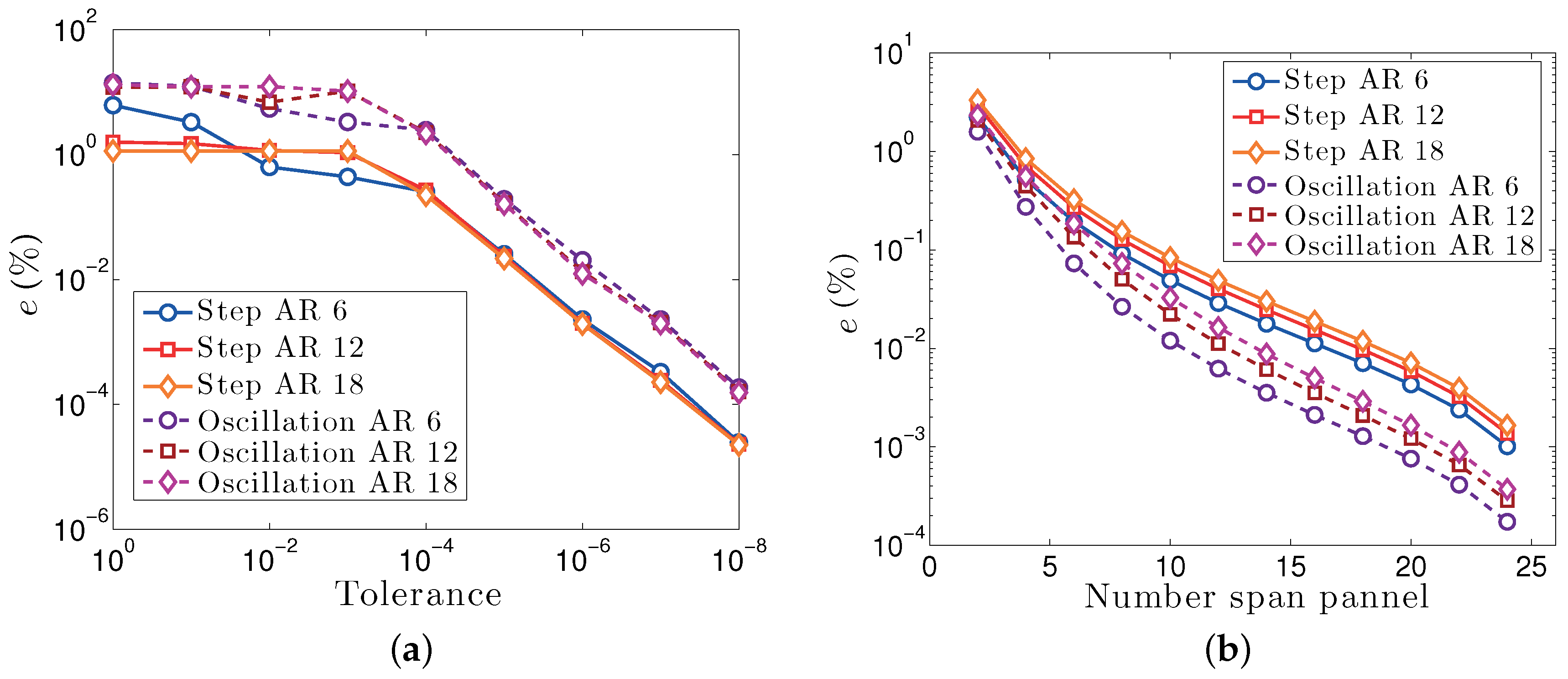
Figure 5 plots the variation of the error of Equation (29) with the tolerance $Tol$ used in the Runge–Kutta–Fehlberg algorithm with respect to a reference $Tol={10}^{-9}$. The solid line represents the convergence for a step case and the dashed line the convergence for a sinusoidal oscillation case with a reduced frequency $k=0.3$. Assuming that $e<0.01\%$ is good accuracy, the figure shows that a tolerance value of ${10}^{-7}$ is sufficient to achieve convergence for both the step and sinusoidal motion.

Figure 5b plots the variation of the error of Equation (29) with the number of strips for different aspect ratios and kinematics with respect to a reference number of strips $m=26$. The time step tolerance is fixed to ${10}^{-7}$. It can be seen that, for all cases, a value of $m=20$ is sufficient to achieve errors $e<0.01\%$. A still acceptable error of $e<0.1\%$ can be achieved with $m=10$ strips. The figure also shows that the higher the $AR$, the greater the number of strips necessary to reach the same level of convergence. As the aspect ratio increases, the spanwise lift distribution becomes flatter and decreases more quickly at the wingtips; the Fourier series of Equation (1) requires more terms in order to represent such lift distributions accurately. In the asymptotic case, a rectangular wing with infinite span can only be modeled if an infinite number of terms is used in the series; we have already shown in Equation (25) that the WLL model then reduces to the classical 2D Wagner formulation.

4.2. Vortex Lattice Convergence

The quality of the solutions obtained from the vortex lattice method is based on the the number of panels used to represent the wing in the spanwise and chordwise directions. The VLM is more sensitive to the chordwise than the spanwise number of panels [30], so a convergence for the number of chordwise panels is performed.

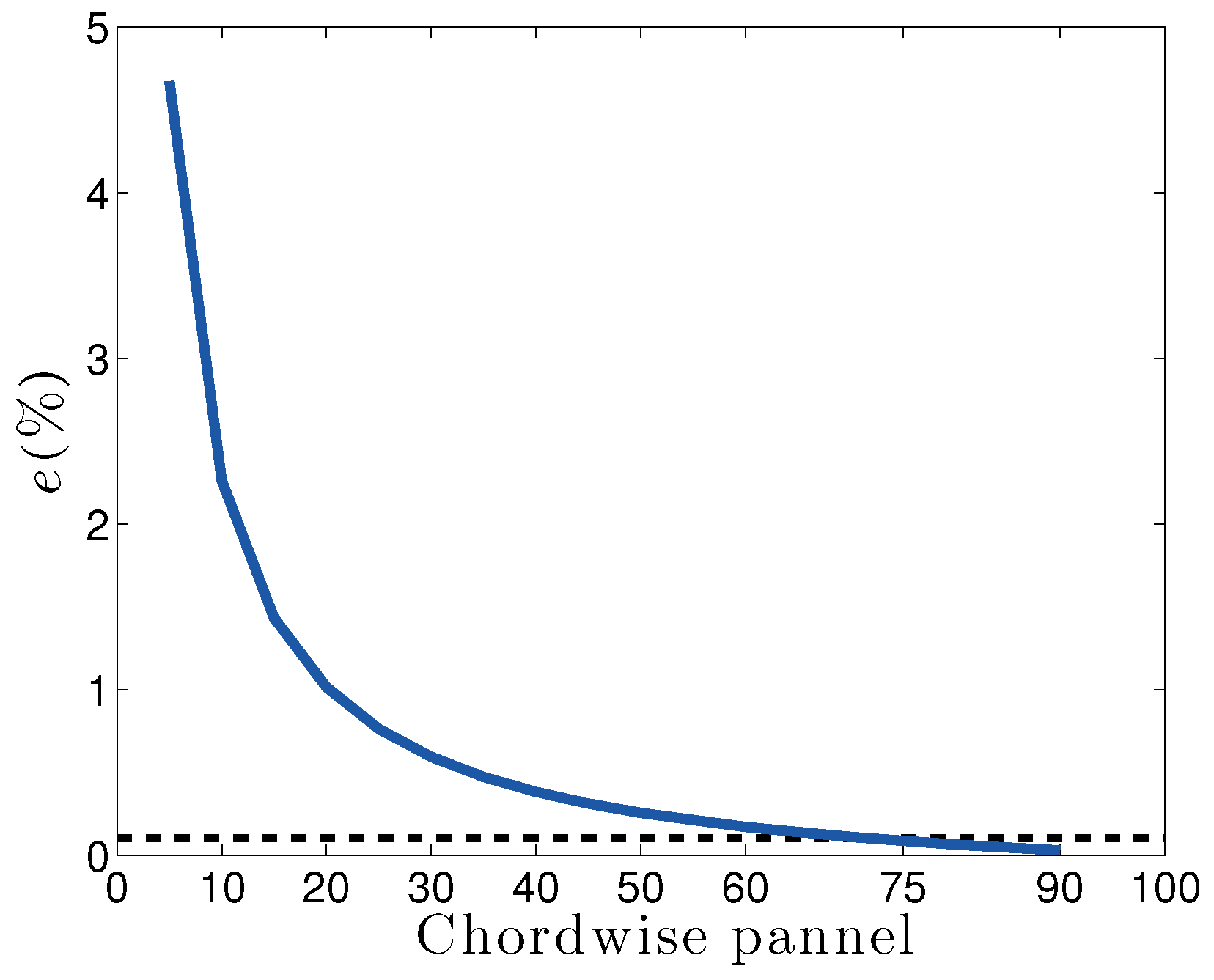
Figure 6 plots the variation of the error of Equation (29) with the number of chordwise panels for a rectangular wing ($AR=6$) oscillating around its leading edge with a reduced frequency $k=0.3$. The reference number of chordwise panels is $j=100$. The number of spanwise panels is set to 15. It can be seen that $j=75$ is sufficient to achieve errors $e<{10}^{-1}\%$ for the rectangular wing case with a leading edge pitch axis. The figure also shows that the convergence is independent of the aspect ratio. This is logical since the convergence parameter is the number of chordwise panels.

All other test cases used in this work converge for $j=75$, as long as the pitch axis does not lie at $c_0/4$. A larger number of chordwise panels $j=100$ is necessary for convergence when the pitch axis lies on the quarter chord because the moment loads need to converge to values very close to zero for the oscillating case with low reduced frequency. Convergence is therefore harder to achieve.

5. Lift and Moment Results for a Rectangular Wing

In this section, the WLL method is applied to the rectangular wing under different kinematic conditions. The lift and moment estimates are compared to predictions obtained by the VLM technique and by strip theory. In all cases, the VLM estimates were obtained from time-converged and spatially-converged simulations.

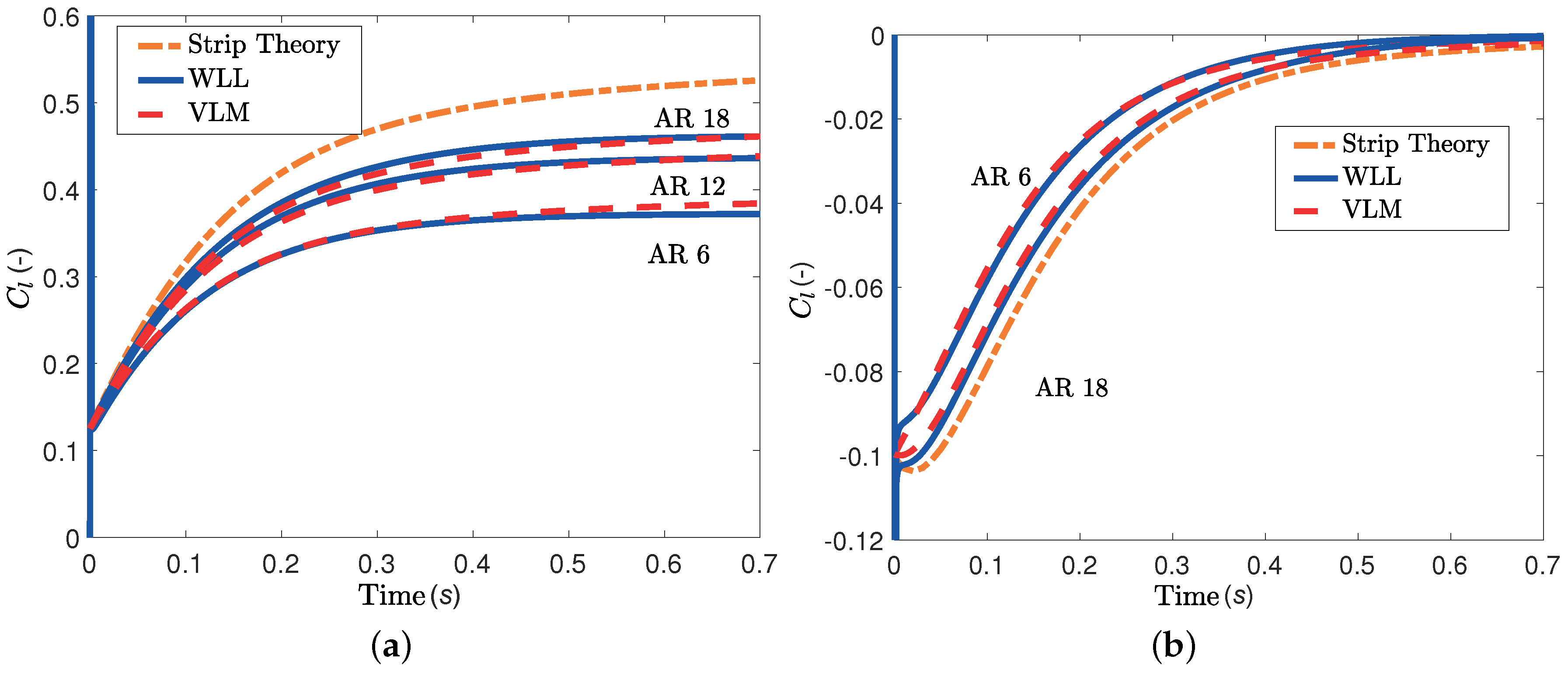
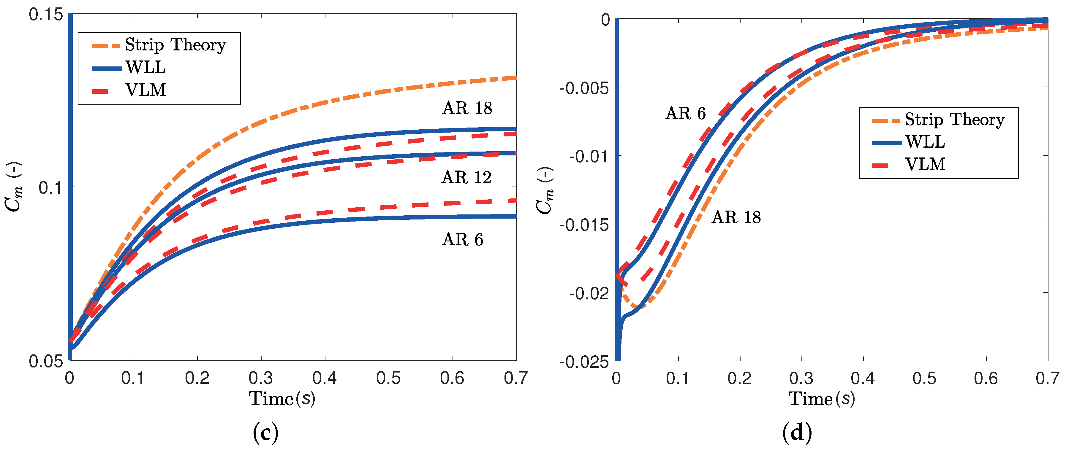
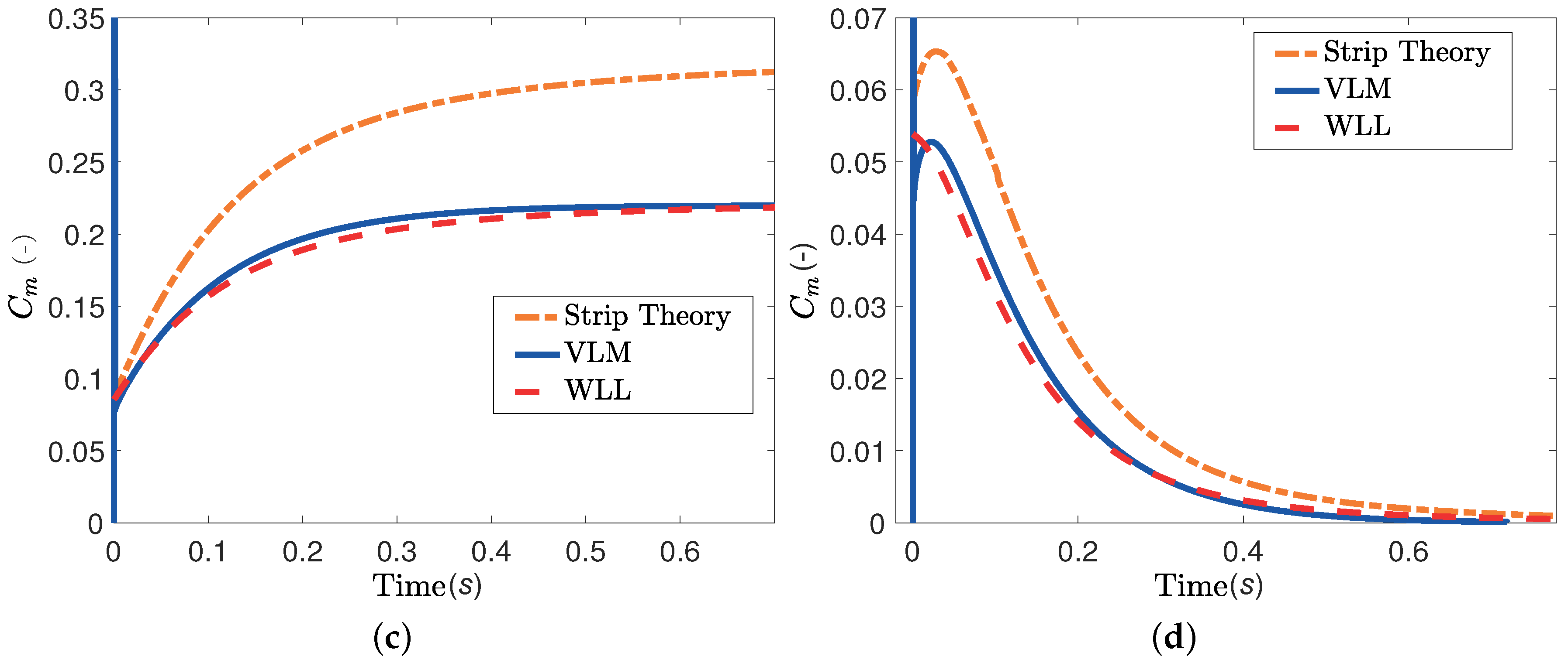
For the first comparison, the pitch axis is located at the leading edge and the wing undergoes a step change in pitch or plunge, as explained in Section 3.1. The resulting lift and moment responses are shown in Figure 7; the WLL estimates are in good agreement with the VLM results for both pitch and plunge motions. In contrast, the strip theory result is significantly overestimated in the pitch step case and underestimated in the plunge step case. Note that the agreement in pitching moment for the step pitch case is not as good as in the other results; small differences between the VLM and WLL predictions persist at steady-state conditions. This is due to modeling differences between the two approaches. WLL calculates the total stripwise lift and places it at the quarter chord. In contrast, the VLM calculates a lift force on the 3/4 chord point of each chordwise panel, and the total stripwise lift is the sum of all the lift forces on the same strip. The point of application of the VLM’s total stripwise lift is exactly the quarter chord only for an infinite number of chordwise panels.

Simulations where repeated for other positions of the pitch axis, but the results are not shown here for conciseness. All of these simulations resulted in WLL predictions that were in good agreement with the VLM estimates.

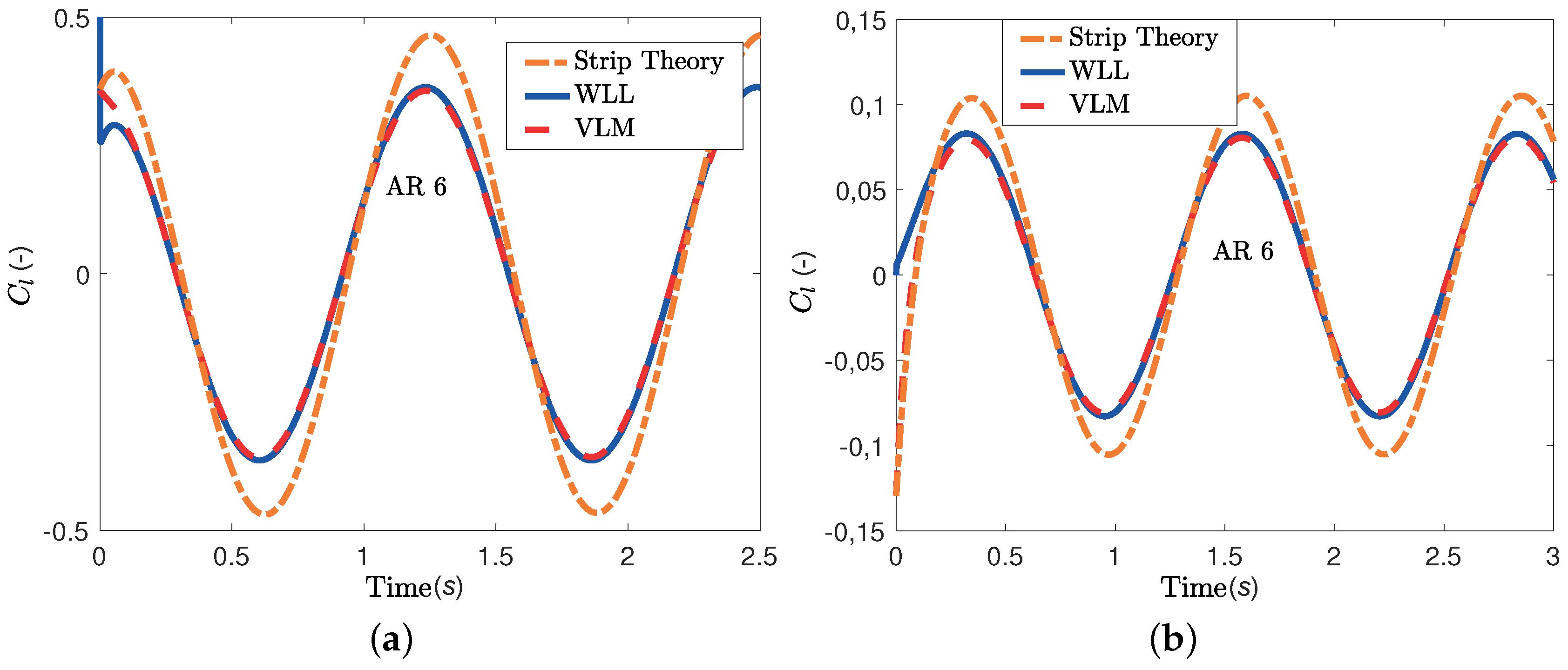
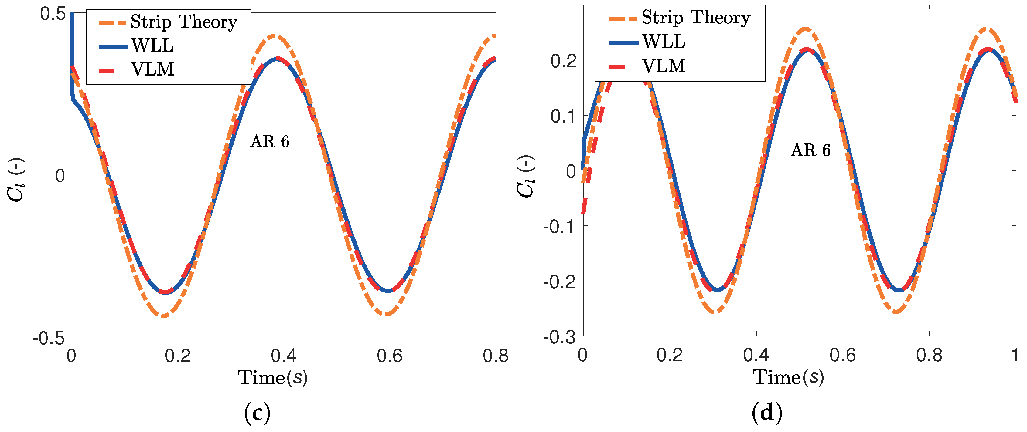
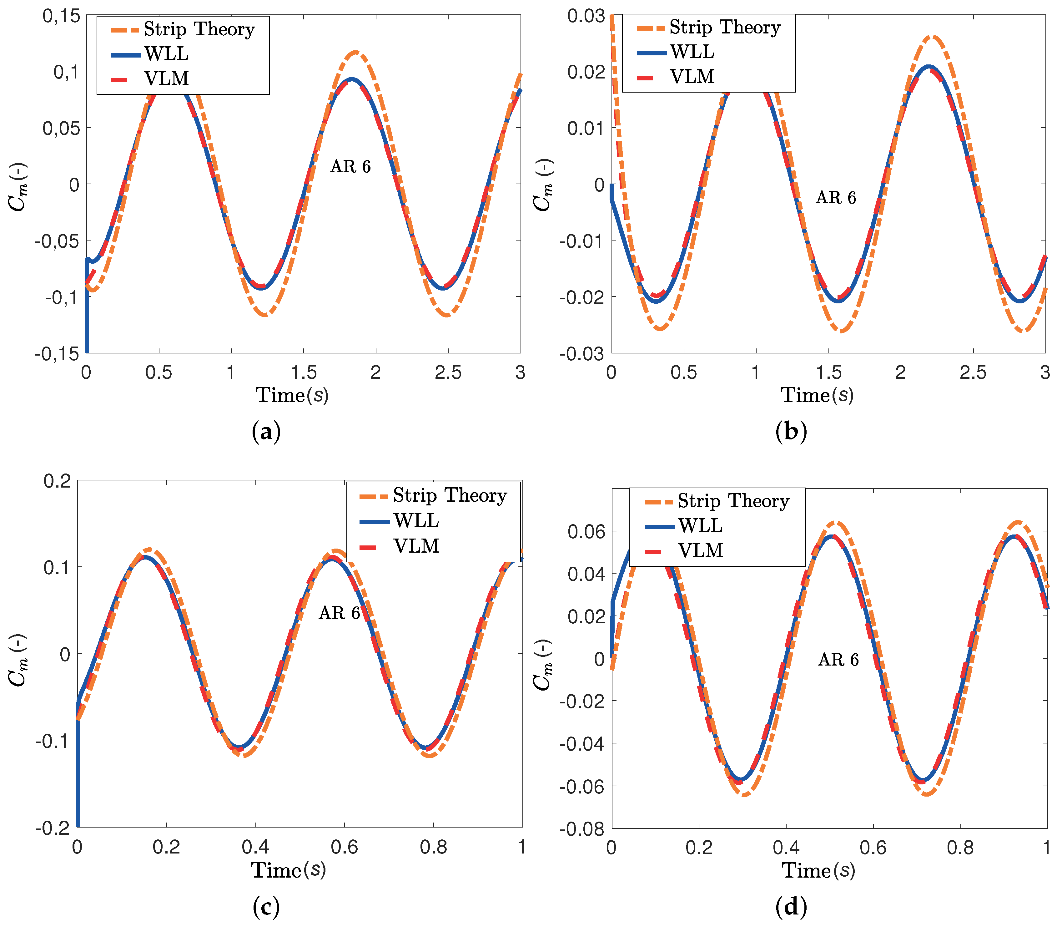
For the second comparison, the WLL, VLM and strip theory techniques are applied to a rectangular wing with an aspect ratio of six undergoing sinusoidal oscillations in pitch or plunge, as detailed in Section 3.1. Several reduced frequency values were tested, but only the results for $k=0.1$ and $k=0.3$ are presented here. The lift results are plotted in Figure 8 and the moment results in Figure 9. There is very good agreement between the WLL and VLM predictions for all frequencies, while the strip theory estimates are quite inaccurate at both values of k.

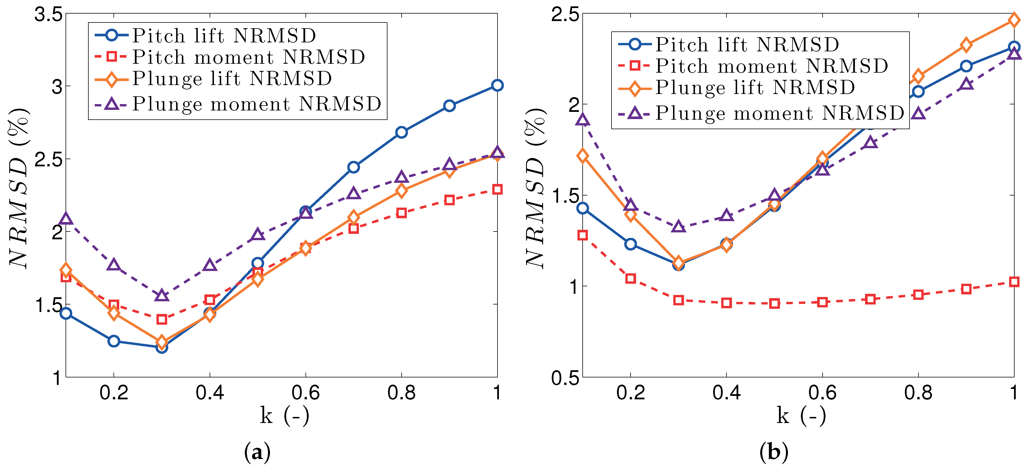
Figure 10a plots the NRMSD values calculated from Equation (27), for all the tested values of k. The difference between the WLL and VLM predictions increases with reduced frequency, but stays lower than 3% for all kinematics and aerodynamic loads. This level of difference is considered good for such frequencies. Repeating the simulations after moving the pitch axis to the quarter chord, as shown in Figure 10b, results in equally good agreement between the WLL and VLM aerodynamic load predictions.

6. Lift and Moment Results for a Tapered Wing

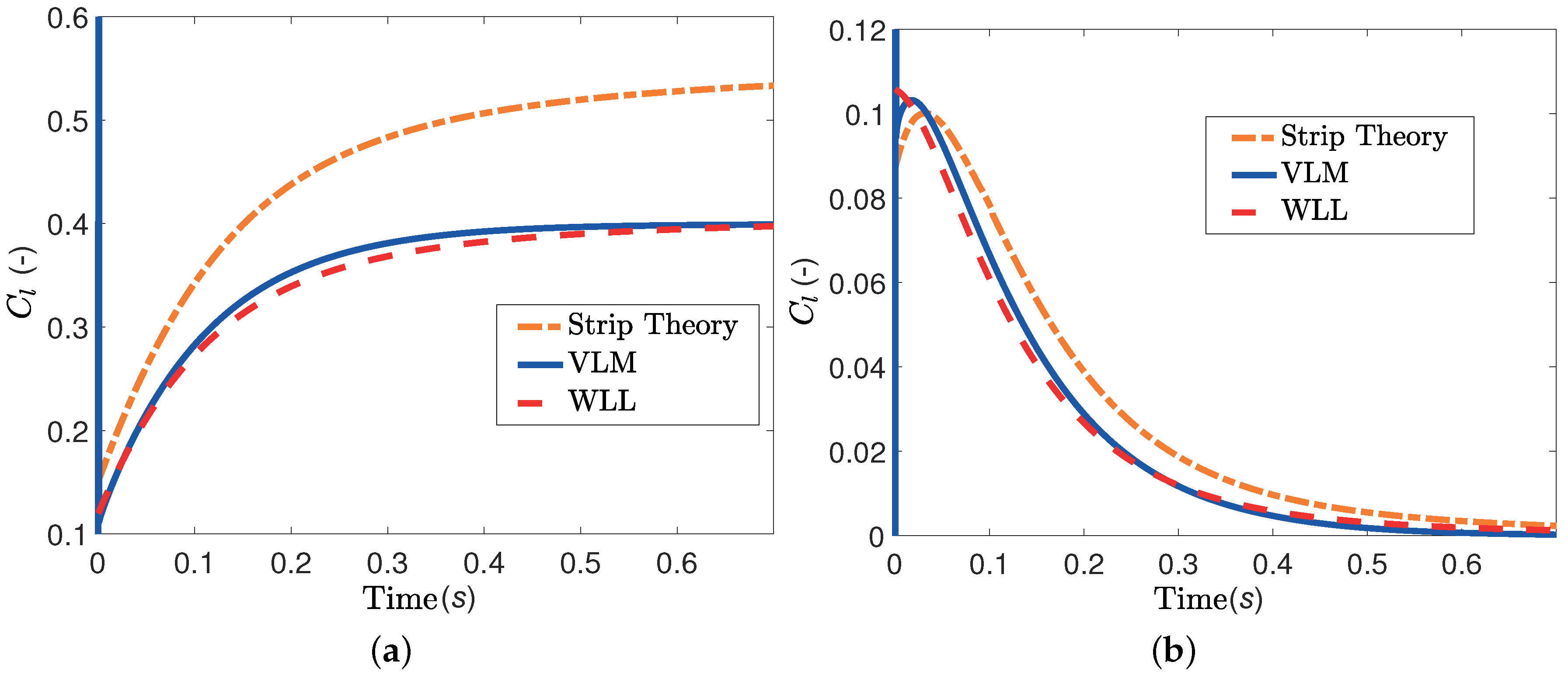
In this section, step and sinusoidal numerical tests are applied to the tapered wing with an aspect ratio of six described in Section 3. Initially, the pitch axis is located at the leading edge of the root chord, and the wing undergoes step changes in pitch or in plunge, as detailed in Section 3.1. The resulting lift and moment responses are shown in Figure 11. In all cases, the WLL and VLM predictions are in very good agreement, while the strip theory results are highly overestimated in the pitch step case. Moving the pitch axis to the quarter chord results in equally good agreement between the WLL and VLM aerodynamic load responses.

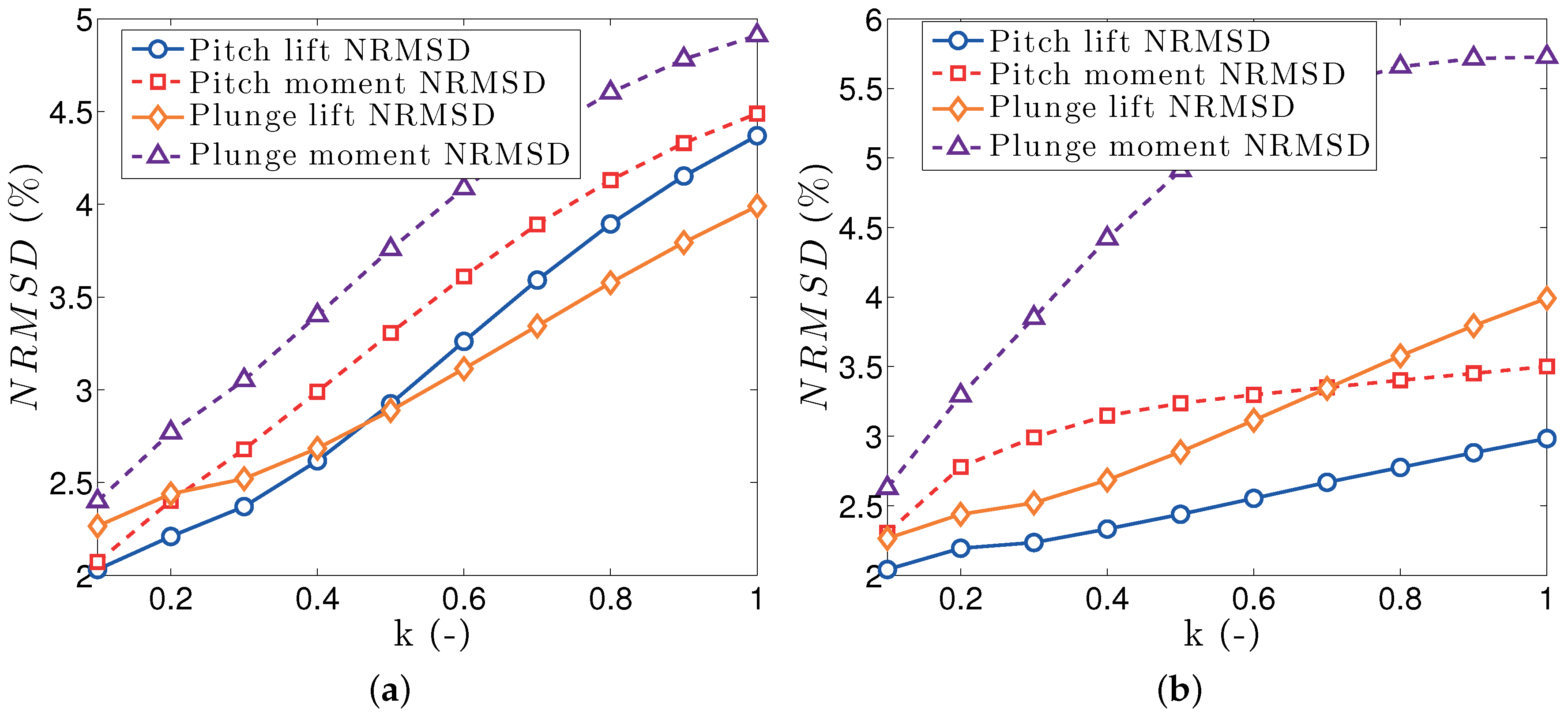
Finally, the WLL and VLM are compared for the case of pitch or plunge sinusoidal oscillations at different reduced frequencies for the tapered wing. The pitch axis is located at the leading edge of the root chord. Figure 12a plots the variation of the NRMSD values between the two sets of predictions, for increasing k values. It can be seen that in all cases the maximum NRMSD stays below 5%. It is concluded that the WLL approach can predict accurately the aerodynamic load responses for oscillating tapered wings. Moving the pitch axis to the quarter chord results in equally good predictions, as seen in Figure 12b.

7. Computational Cost

The computation times of the WLL and VLM approaches are compared for a step and three sinusoidal oscillations in pitch, with reduced frequencies $k=[0.1,0.5,1]$ and a total simulation time $T_f=1.3$ s. The following parameters have been used for each method:

VLM: 

There are 15 spanwise and 20 chordwise panels, and the time step is $\Delta t={10}^{-3}$. The wake shape is prescribed in order to reduce computational cost.

WLL: 

The computation parameters used are 15 strips, a tolerance $Tol={10}^{-8}$ and an initial time step $\Delta t={10}^{-3}$ for the Runge–Kutta–Fehlberg 45 algorithm.

All the calculations were run on a MacBook Pro laptop computer with a quad-core Intel i7 processor rated at $2.5$ GHz, running iOS Version 10.9.5.

Table 1. Computation time comparison between VLM and WLL.

Model	Step	Oscillation $\mathit{k}=0.1$	Oscillation $\mathit{k}=0.5$	Oscillation $\mathit{k}=1$
VLM	503 s	504 s	495 s	497 s
WLL	15 s	36 s	57 s	32 s

shows that WLL calculation times are much lower than VLM numerical simulations to simulate $1.3$ s of pitch step or sinusoidal oscillations with reduced frequency $k=[0.1,0.5,1]$. The benefit of an adaptive time step for WLL can also be seen as the computation time is lower for cases with low or high reduced frequencies. It should be stressed that the implementation of the two methods is completely different; the WLL is implemented purely in MATLAB, while the VLM is implemented as a combination of MATLAB and C code (mex functions). If the WLL were also implemented using compiled code, it would be even faster.

8. Aeroelastic Test Case

In order to further validate the Wagner lifting line approach, an aeroelastic test case is presented for a rigid rectangular wing with pitch and plunge degrees of freedom. The flutter speed will be computed as a function of the position of the pitching axis and the wing’s aspect ratio using both the Wagner lifting line and the Vortex lattice method.

8.1. Aeroelastic Equations of Motion

The structure simply consists of a rigid wing with two degrees of freedom in pitch and plunge. The structural equations of motion are given by:

$$\begin{array}{c}\hfill \left[\begin{array}{cc}{m}_w& S_w\\ S_w& I_w\end{array}\right]\ddot{\mathbf{q}}+\left[\begin{array}{cc}{k}_h& 0\\ 0& k_{\alpha }\end{array}\right]\mathbf{q}=\left[\begin{array}{c}-L(t)\\ M(t)\end{array}\right]\end{array}$$

(30)

where $\mathbf{q}={\left[h\alpha \right]}^T$, h is the plunge displacement, $\alpha$ the pitch displacement, $m_w$ the mass, $S_w$ the static imbalance around the pitching axis, $I_w$ the moment of inertia around the pitching axis, $k_h$ and $k_{\alpha }$ the stiffnesses of the springs providing restoring loads in the plunge and pitch degrees of freedom, respectively, and $L(t)$ and $M(t)$ are the lift and moment around the pitching axis computed using the VLM or WLL approaches.

The wing is chosen as an aluminum rectangular flat plate with chord $c_0=0.1$ m, thickness $h=0.005$ m and span s; the distance between the pitch axis and the mid-chord is $x_e$. The mass matrix components can then be computed as:

$$\begin{array}{ccc}\hfill m_w& =& {\rho }_{al}sh{c}_0\hfill \\ \hfill I_w& =& \frac{m_w{c}_0^2}{12}+m_w{c}_0^2{x}_e^2\hfill \\ \hfill S_w& =& -m_w{x}_e\hfill \end{array}$$

where ${\rho }_{al}=2300$ kg/m${}^3$ is the density of aluminum. The spring stiffnesses for the two degrees of freedom are chosen such that the uncoupled, wind-off natural frequencies of the system are $f_h=1$ Hz and $f_{\alpha }=5$ Hz. The stiffnesses are then given by:

$$\begin{array}{ccc}\hfill k_h& =& m_w{\left(2\pi f_h\right)}^2\hfill \\ \hfill k_{\alpha }& =& I_w{\left(2\pi f_{\alpha }\right)}^2\hfill \end{array}$$

The normal force $L(t)$ and moment around the pitching axis $M(t)$ are computed from Equations (6) and (8), together with the added mass effects described in Expressions (20) and (21). The integrals are approximated using the trapezoidal rule.

Finally, the complete linear aeroelastic system composed of Equations (30) and (22) can be written in first-order form as:

$$\begin{array}{c}\hfill \dot{\mathbf{x}}=\mathbf{H}(U,x_e)\mathbf{x}\end{array}$$

(31)

The aeroelastic system matrix $\mathbf{H}$ is derived in Appendix A, while $\mathbf{x}$ represents the system states and is defined as:

$$\mathbf{x}={\left[\begin{array}{cccccccc}{a}_1& \dots & a_m& {\mathbf{z}}_1& \dots & {\mathbf{z}}_m& \mathbf{q}& \dot{\mathbf{q}}\end{array}\right]}^T$$

(32)

where $a_i$ is the i-th Fourier coefficient, ${\mathbf{z}}_i$ are the local aerodynamic state variables for the i-th strip:

$${\mathbf{z}}_i=\left[\begin{array}{cccccc}{z}_{i,1}& z_{i,2}& z_{i,3}& z_{i,4}& z_{i,5}& z_{i,6}\end{array}\right]$$

$\mathbf{q}=\left[h\alpha \right]$ and m is the number of strips. Consequently, the total number of states is 7m + 4.

Finally, the WLL flutter solution is obtained by computing the eigenvalues of matrix $\mathbf{H}(U,x_e)$ as a function of the airspeed U. An indirect search procedure is employed to pinpoint the airspeed at which one pair of complex conjugate eigenvalues becomes purely imaginary, which is the definition of the flutter speed. The number of strips used to estimate matrix $\mathbf{H}(U,x_e)$ is $m=20$, and the flutter solution is obtained for several values of the position of the pitch axis $x_e$.

The VLM flutter solution is obtained using the modal frequency domain version of the method, as detailed in [11]. Rigid body modes are chosen, one for the plunge and one for the pitch. The mode shapes are given by:

$$\begin{array}{ccc}\hfill w_h(x,y)& =& 1\hfill \\ \hfill w_{\alpha }(x,y)& =& x\hfill \end{array}$$

where $w_h(x,y)$ is the plunge mode shape and $w_{\alpha }(x,y)$ the pitch mode shape. The elements of the mass matrix are then obtained from:

$$\begin{array}{ccc}\hfill m_w& =& {\rho }_{al}h{\int }_0^c{\int }_0^y{w}_h^2(x,y)\mathrm{d}x\mathrm{d}y\hfill \\ \hfill I_w& =& {\rho }_{al}h{\int }_0^c{\int }_0^y{w}_{\alpha }^2(x,y)\mathrm{d}x\mathrm{d}y\hfill \\ \hfill S_w& =& {\rho }_{al}h{\int }_0^c{\int }_0^y{w}_h(x,y)w_{\alpha }(x,y)\mathrm{d}x\mathrm{d}y\hfill \end{array}$$

The resulting flutter problem is of the form:

$$\left({\left(\frac{kU}{b}\right)}^2\mathbf{A}\ddot{\mathbf{q}}+\mathbf{Eq}-\rho U^2\mathbf{Q}(k)\right)\mathbf{q}(k)=0$$

(33)

where ${\mathbf{A}}_s$ is the structural mass matrix, ${\mathbf{E}}_s$ is the structural stiffness matrix and $\mathbf{Q}(k)$ is the frequency-dependent generalized aerodynamic force matrix generated by the VLM approach. The flutter problem is solved using the $p-k$ method.

8.2. Results

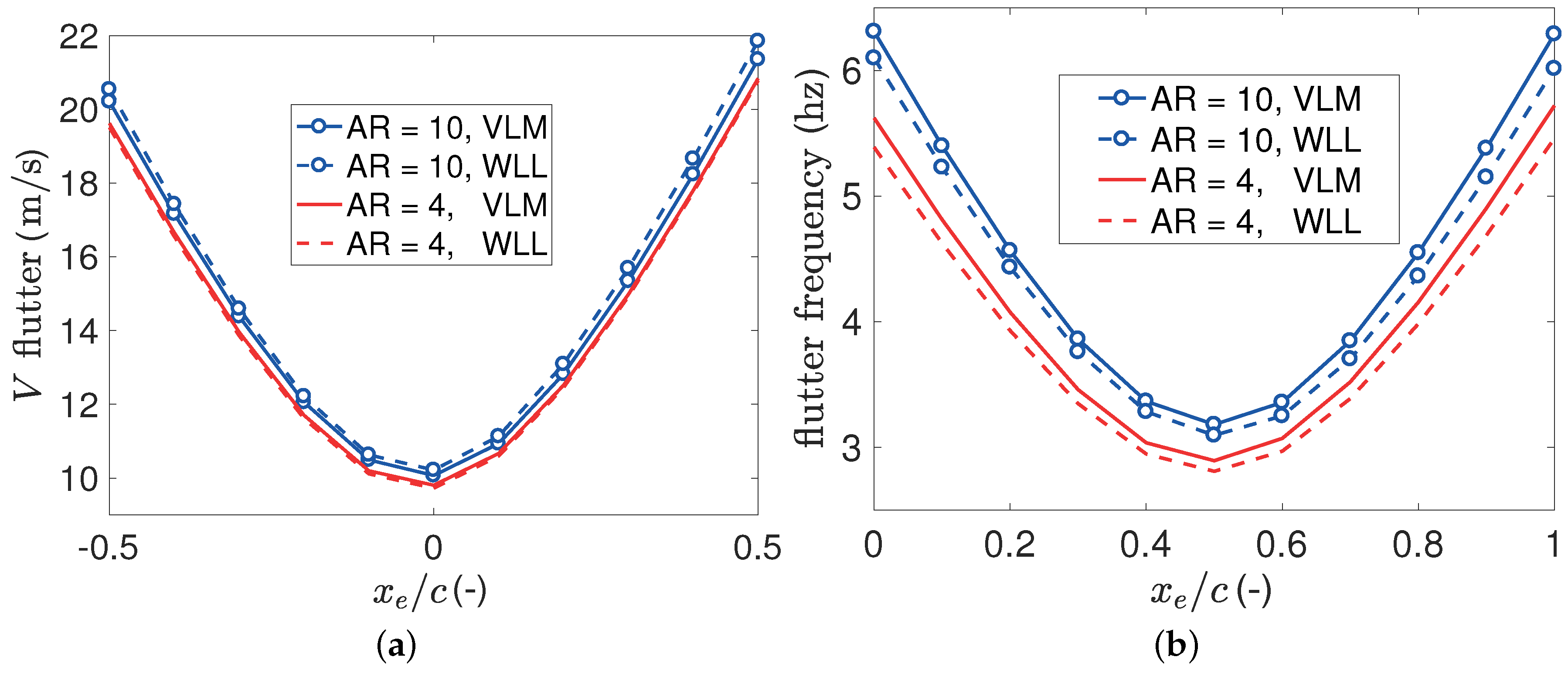
The resulting flutter speed and frequency values are plotted against the position of the pitch axis in Figure 13 for two aspect ratios: $AR=4$ and $AR=10$. Figure 13a plots the flutter airspeeds and shows that the VLM and WLL predictions are in good agreement with each other for both aspect ratios. Figure 13b plots the flutter frequency predictions; the agreement is still very good as the highest frequency discrepancy is of the order of 5%. It can be concluded that the Wagner lifting line method can predict accurately the flutter of a wing with a finite span.

9. Conclusions

The WLL method results in a closed-form, state-space representation of the unsteady aerodynamic loads acting on finite rectangular and tapered wings of different aspect ratios, under attached incompressible flow conditions. The technique combines Wagner’s 2D unsteady lift theory, Prandtl’s lifting line theory, the unsteady Kutta–Joukowski theorem and the added mass terms from Theodorsen’s analysis. Sample simulations on wings with and without taper have shown very good agreement between the WLL predictions and VLM simulation results. The method can also be readily applied to wings with twist and camber. Sweep is more problematic, since lifting line theory has to be modified in order to work in the presence of sweep. This modification will be addressed in future work.

The VLM approach is still more general than the WLL technique, as it can easily represent sweep. The advantage of WLL is the fact that the resulting aerodynamic loads are written in state space form, as functions of the structural and aerodynamic states. They can therefore be easily included in aeroelastic and flight dynamic calculations. In contrast, the VLM or DLM techniques result in time-marching simulations or, if using a modal frequency domain technique, in Equation (33), which is a hybrid time-frequency domain equation that must be transformed to the time domain in order to carry out aeroservoelastic calculations. In the present examples, the wings were rigid with discrete degrees of freedom, but flexible wings with generalized modes can also be treated. Finally, the WLL calculations are significantly faster than time domain VLM numerical simulations.

References

- Theodorsen, T. General Theory of Aerodynamic Instability and the Mechanism of Flutter; Technical Report NACA TR-496; NACA: Washington, DC, USA, 1935.
- Jones, R.T. The Unsteady Lift of a Finite Wing; Technical Report NACA TN-682; NACA: Washington, DC, USA, 1939.
- Fung, Y.C. An Introduction to the Theory of Aeroelasticity; Dover Publications: Mineola, NY, USA, 1993. [Google Scholar]
- Peters, D.A.; Karunamurthy, S.; Cao, W.M. Finite state induced flow models; Part I: Two-dimensional thin airfoil. J. Aircr. 1995, 32, 313–322. [Google Scholar] [CrossRef]
- Leishman, J.; Nguyen, K. State-space representation of unsteady airfoil behavior. AIAA J. 1990, 28, 836–844. [Google Scholar] [CrossRef]
- Dowell, E.H. (Ed.) A Modern Course in Aeroelasticity, 4th ed.; Kluwer Academic Publishers: Dordrecht, The Netherlands, 2004. [Google Scholar]
- Albano, E.; Rodden, W.P. A Doublet-Lattice Method for Calculating Lift Distributions on Oscillating Surfaces in Subsonic Flows. AIAA J. 1969, 7, 279–285. [Google Scholar] [CrossRef]
- Katz, J.; Plotkin, A. Low Speed Aerodynamics; Cambridge University Press: Cambridge, UK, 2001. [Google Scholar]
- Karpel, M. Design for the Active Flutter Suppression and Gust Alleviation Using State-Space Aeroelastic Modeling. J. Aircr. 1982, 19, 221–227. [Google Scholar] [CrossRef]
- Dimitriadis, G. Introduction to Nonlinear Aeroelasticity; John Wiley & Sons, Inc.: Chichester, UK, 2017. [Google Scholar]
- Dimitriadis, G.; Giannelis, N.F.; Vio, G.A. A Modal Frequency-Domain Generalised Force Matrix for the Unsteady Vortex Lattice Method. J. Fluids Struct. 2018, 76, 216–228. [Google Scholar] [CrossRef]
- Reissner, E. Boundary value problems in aerodynamics of lifting surfaces in non-uniform motion. Bull. Am. Math. Soc. 1949, 55, 825–850. [Google Scholar] [CrossRef]
- Chopra, M.G. Hydromechanics of lunate-tail swimming propulsion. J. Fluid Mech. 1974, 64, 375–391. [Google Scholar] [CrossRef]
- Chopra, M.G.; Kambe, T. Hydromechanics of lunate-tail swimming propulsion. Part 2. J. Fluid Mech. 1977, 79, 49–69. [Google Scholar] [CrossRef]
- James, E.C. Lifting-line theory for an unsteady wing as a singular perturbation problem. J. Fluid Mech. 1975, 70, 753–771. [Google Scholar] [CrossRef]
- Ahmadi, A.R.; Widnall, S.E. Unsteady lifting-line theory as a singular perturbation problem. J. Fluid Mech. 1985, 153, 59–81. [Google Scholar] [CrossRef]
- Van Holten, T. Some notes on unsteady lifting line theory. J. Fluid Mech. 1976, 77, 561–579. [Google Scholar] [CrossRef]
- Phlips, P.J.; East, R.A.; Pratt, N.H. An unsteady lifting line theory of flapping wings with application to the forward flight of birds. J. Fluid Mech. 1981, 112, 97–125. [Google Scholar] [CrossRef]
- Dragos, L. The Theory of Oscillating Thick Wings in Subsonic Flow. Lifting Line Theory. Acta Mech. 1985, 54, 221–238. [Google Scholar] [CrossRef]
- Sclavounos, P.D. An unsteady lifting-line theory. J. Eng. Math. 1987, 21, 201–226. [Google Scholar] [CrossRef]
- Drela, M. Integrated simulation model for preliminary aerodynamic, structural, and control-law design of aircraft. Am. Inst. Aeronaut. Astronaut. 1999. [Google Scholar] [CrossRef]
- Nabawy, M.; Crowther, W.J. On the quasi-steady aerodynamics of normal hovering flight part II: Model implementation and evaluation. J. R. Soc. Interface 2014, 11, 20131197. [Google Scholar] [CrossRef] [PubMed]
- Nabawy, M.; Crowther, W.J. A Quasi-Steady Lifting Line Theory for Insect-Like Hovering Flight. J. R. Soc. Interface 2015, 10, e0134972. [Google Scholar] [CrossRef] [PubMed]
- Boutet, J.; Dimitriadis, G. Unsteady lifting line theory using the Wagner function. In Proceedings of the 55th AIAA Aerospace Sciences Meeting, Grapevine, TX, USA, 9–13 January 2017. [Google Scholar]
- Izraelevitz, J.S.; Zhu, Q.; Triantafyllou, M.S. State-Space Adaptation of Unsteady Lifting Line Theory: Twisting/Flapping Wings of Finite Span. AIAA J. 2017, 55, 1279–1294. [Google Scholar] [CrossRef]
- Kuethe, A.M.; Chow, C.Y. Foundations of Aerodynamics: Bases of Aerodynamic Design, 4th ed.; Wiley: New York, NY, USA, 1986. [Google Scholar]
- Glauert, H. The Elements of Aerofoil and Airscrew Theory, 2nd ed.; Cambridge Science Classics; Cambridge University Press: Cambridge, UK, 1983. [Google Scholar]
- Jones, R.T. Operational Treatment of the Nonuniform-Lift Theory in Airplane Dynamics; Technical Report NACA TN-667; NACA: Washington, DC, USA, 1938.
- Dimitriadis, G.; Gardiner, J.; Tickle, P.; Codd, J.; Nudds, R. Experimental and numerical study of the flight of geese. Aeronaut. J. 2015, 119, 1–30. [Google Scholar] [CrossRef]
- Simpson, R.J.S.; Palacios, R. Induced-Drag Calculations in the Unsteady Vortex Lattice Method. AIAA J. 2013, 51, 1775–1779. [Google Scholar] [CrossRef]
Figure 1.
Rigid thin plate airfoil scheme.
Figure 2.
Representation of m strips along the wing span and their respective local variables.
Figure 3.
Rectangular wing with pitch axis at the leading edge and quarter chord.
Figure 4.
Tapered wing with pitch axis at the leading edge and quarter chord.
Figure 5.
Wagner Lifting Line (WLL) convergence with the tolerance parameter and number of spanwise strips for a rectangular wing. (a) Tolerance parameter; (b) Number of spanwise strips.
Figure 6.
Vortex Lattice Method (VLM) convergence with the number of chordwise panels.
Figure 7.
Comparison between VLM, WLL and strip theory for a rectangular wing undergoing a step motion. (a) Lift coefficient, pitch step A = 5° (b) Lift coefficient, plunge step A = 0.1 m; (c) Moment coefficient, pitch step A = 5°; (d) Moment coefficient, plunge step A = 0.1 m.
Figure 8.
Lift comparison between VLM, WLL and strip theory for a rectangular wing undergoing an oscillation motion. (a) Oscillation in pitch with A = 5° and k = 0.1; (b) Oscillation in plunge with A = 0.1 m and k = 0.1; (c) Oscillation in pitch with A = 5° and k = 0.3; (d) Oscillation in plunge with A = 0.1 m and k = 0.3.
Figure 9.
Moment comparison between VLM, WLL and strip theory for a rectangular wing undergoing an oscillation motion. (a) Oscillation in pitch with and ; (b) Oscillation in plunge with m and ; (c) Oscillation in pitch with and ; (d) Oscillation in plunge with m and .
Figure 10.
NRMSD between VLM and WLL aerodynamic responses for a rectangular wing undergoing oscillations motion. (a) Pitch axis on leading edge; (b) Pitch axis on quarter chord.
Figure 11.
Comparison between VLM, WLL and strip theory for a tapered wing, AR = 6, undergoing a step motion. (a) Lift coefficient, pitch step A = 5°; (b) Lift coefficient, plunge step A = 0.1 m; (c) Moment coefficient, pitch step A = 5°; (d) Moment coefficient, plunge step A = 0.1 m.
Figure 12.
NRMSD between VLM and WLL aerodynamic responses for a tapered wing undergoing oscillations motion. (a) Pitch axis on root leading edge; (b) Pitch axis on root quarter chord.
Figure 13.
Comparison of flutter with the aeroelastic axis for a 3D wing, computed with vortex lattices (dashed line) and the Wagner lifting line (solid). (a) Flutter speed; (b) Flutter frequency.