Analysis of Coherent Structures in an Under-Expanded Supersonic Impinging Jet Using Spectral Proper Orthogonal Decomposition (SPOD)

Abstract

The spatiotemporal dynamics of the coherent structures in an under-expanded supersonic impinging jet are studied using a spectral proper orthogonal decomposition technique. For this analysis, a large eddy simulation of an under-expanded supersonic impinging jet at a pressure ratio of 3.4 and a stand-off distance of 2 jet diameters at a Reynolds number of 50,000 is performed. The mean flow fields illustrate some striking features of this flow, such as an oblique shock, a stand-off shock, a Mach disk, and a recirculation bubble. The spectral proper orthogonal decomposition method is applied to time-resolved three-dimensional flow fields. The accumulative energy of modes within each azimuthal mode number reveals that the first three azimuthal modes contain most of the energy of the flow. The spectra of these azimuthal modes show that the flow exhibits a low-ranked behaviour with discrete frequencies at the optimal symmetric azimuthal mode while other two azimuthal modes have negligible contributions in this behaviour. Three peaks are observed in the spectra of the optimal symmetric azimuthal mode. The spatial fields of the streamwise velocity and pressure of these peaks show that the complex structures are consequences of the under-expansion, Mach disk, and the impingement. Strong hydrodynamic instabilities exist in the shear layer of the jet in the optimal azimuthal mode at each of these dominant frequencies. High-amplitude acoustic waves are also present in the near-field of the jet. These acoustic waves are strong at the nozzle lip, suggesting that a feedback loop linking these two processes exists for dominant frequencies in the optimal mode. High cross-spectrum density of near-field pressure fluctuations and streamwise velocity fluctuations near the nozzle lip at these frequencies confirms the hydro-acoustic coupling, which is necessary to close the feedback loop.

1. Introduction

A supersonic jet impinging normally on a flat plate generates very intense tones which depend on both the jet exit flow conditions and the nozzle-to-wall distance. The interactions of these acoustic waves and flow create self-sustained oscillations. These oscillations of the flow have been observed in subsonic impinging jets, a resonance tube, an edge-tone, and a plate with a cavity [1]. The first attempt to shed light on these oscillations in supersonic jets was the experimental Schlieren study of under-expanded jets impinging on a plate by Powell [2], in which it was observed that the disturbances were convected by the vortex in the jet shear layer and interacted directly with the impinging plate. This interaction generates acoustic waves. The upstream propagation of these acoustic waves triggers the flow at the nozzle lip and initialises a shear layer instability. This mechanism is commonly referred to as an acoustic feedback loop. Henderson and Powell [3] modified the feedback loop to include the effect of shock waves, which was neglected in their previous study [2]. The modified feedback loop is more complex as the convected disturbances interact with shock waves. This interaction results in displacements of the shock waves and the production of sound waves. These sound waves are reflected by the impinging wall and once again interact with the shock waves. The sound waves are also distorted by the shock waves. They reach the nozzle lip and close the loop by initialising shear layer instabilities. The experimental investigations by Powell [2] and Henderson and Powell [3] revealed two main acoustic wave sources. One is the shock oscillations, while the other is a vortex–wall interaction. In both mechanisms, the main parts of the feedback loop are the shear layer instabilities propagating downstream and pressure waves propagating upstream. The shear layer instabilities form unstable spatially growing hydrodynamic waves, and have been observed in previous experimental and numerical studies of free and impinging under-expanded supersonic jets [2,4,5,6,7,8,9,10]. There is a common belief that the acoustic waves scattered by the nozzle lip through the receptivity process internalise as shear layer Kelvin–Helmholtz-type instabilities and form these coherent structures [2,11,12]. The near-field acoustic fields of these flows have also been studied experimentally [2,4,6,7,10], where the upstream propagating acoustic waves were visualised using the Schlieren technique. What is known about the feedback loop is largely based on these observations, but the connection between the formation of the coherent structures and sound generation are not well understood. This is mainly due to lack of simultaneous measurements of acoustic and flow fields in experimental studies and a well-established post-processing technique in numerical studies.

In recent years, there has been considerable interest in data-driven techniques to reveal the characteristics of coherent structures, especially in jet flows [13,14,15,16,17,18]. In the recent series of large eddy simulation studies of ideally expanded and under-expanded supersonic slot and round impinging jets [5,8,19], the discrete Fourier transform of the near-field pressure has been used to obtain the frequencies of the acoustic tones. The predicted acoustic tones and mean flow fields were in a good agreement with the experimental and numerical study of Krothapalli [20] for the ideally expanded jets, and with the experimental results of Henderson et al. [3,12] for the under-expanded supersonic impinging case. In the experiment of under-expanded free jets by Edgington-Mitchell et al. [10], proper orthogonal decomposition (POD) was applied to the radial velocity field to obtain the most energetic modes. In another study of an under-expanded supersonic jet impinging on a cylindrical surface by Weightman et al. [21], a combination of POD analysis of the flow field obtained from a (particle image velocimetry (PIV) measurement and the sound measurement by a microphone was used to explain the phase lag term in Powell’s formula [2]. Dynamic mode decomposition (DMD) is a more recent data-driven approach proposed by Schmid [16], where the flow field is decomposed into modes, with each mode having a growth/decay rate at a single frequency. A fundamental issue of POD, DMD, and Fourier decomposition is their weakness in identifying coherent structures when they have low energy or multiple frequencies [13]. More recently, spectral proper orthogonal decomposition (SPOD) was revitalised by Towne et al. [13]. SPOD is based on the original decomposition method of Lumley [22], where the flow is decomposed into energy-ranked spatial modes at discrete frequencies. The authors presented a comprehensive study on the advantages of SPOD over other data-driven methods like POD and DMD and their connections. Note that the SPOD method of Lumley [22] has previously been applied to an experimental hot wire measurement of the velocity in the shear layer of an axisymmetric jet by Glauser et al. [23]. The authors used the decomposition method of Lumley to study the coherent structures in an axisymmetric jet, and showed that the nearly all the energy of the flow was in the first three modes. In another study by Delville et al. [24], this approach was used to study the coherent structures in an experimental study of a plane turbulent mixing layer where the first mode was found to be dominant and it contained nearly 50% of the turbulent kinetic energy.

In this paper we use SPOD to decompose the flow field and study the coherent structures in space and time as a function of frequency. This is used to explain the forward and backward paths of the feedback loop, representing the hydrodynamic instability in the shear layer of the jet and the acoustic wave propagating in the medium, respectively. Models have been developed to predict the frequency in which these two processes are coupled. However, to the best of authors’ knowledge, there is no analysis of the structure of the flow as a function of frequencies available in the literature. A large eddy simulation is performed to obtain a time-resolved flow field. The three-dimensional snapshots of the primitive variables in the entire domain are used for the purpose of SPOD analysis. The structures of the dominant frequencies in the optimal mode are presented.

The rest of the paper is organised as follows: first, the configuration, numerical method, and theory of the SPOD are briefly described. Next, the first- and second-order statistics of the flow field are presented. This is followed by the presentation of the results of SPOD analysis. Finally, concluding remarks are provided.

2. Configuration

The configuration is an under-expanded impinging jet with a nozzle-to-wall distance of 2d and a radial domain of 12d, where d is the jet diameter. There are $N_x\times N_r\times N_{\theta }=480\times 400\times 96$ computational grid points in the large eddy simulation (LES). A uniform grid is employed in the azimuthal direction. In the axial direction, stretch grid points are used with two stretching rates. A fine grid is used near the nozzle and the impinging wall. A fine grid point is employed in the mixing layer, with a polynomial stretch of the grids towards the centre of the jet and far-field. The grid is examined carefully to make sure the resolution was adequate, especially in the shear layer and near the walls. The locations of the radial and axial grids are shown in Figure 1 for the sake of completeness. There are 80 grid points in the shear layer region of the jet, which is considered to be enough for the purposes of this study.

The mean inlet axial velocity $U_{in}$ is specified using the hyperbolic-tangent function Ref. [25] given by

$$\begin{array}{c}\hfill \frac{U_{in}}{U_j}=\frac{1}{2}\left(1-tanh\left[\frac{1}{4{\delta }_{in}}(\frac{r}{r_j}-\frac{r_j}{r})\right]\right),\end{array}$$

(1)

where $U_j$ is the jet inlet velocity, $r_j$ the jet inlet radius, and ${\delta }_{in}$ the inlet momentum (mixing layer) thickness. The inlet momentum thickness is equal to $0.04d_j$ in this simulation. The inlet velocity is free of any synthetic turbulence. The Reynolds number based on jet diameter and air velocity in the inlet is 50,000, the Mach number is 1.0, and the ratio between the stagnation pressure measured in the jet plenum and the ambient pressure or nozzle pressure ratio (NPR) is 3.4. The flow condition examined in this study is similar to the experimental study of Weightman et al. [21]. Only the Reynolds number differs from the experiment. An approximately order of magnitude lower Reynolds number is chosen to maintain the LES resolution requirement under acceptable computational cost [26]. The simulation is run for 200 acoustic time units ($ta/d_j$, where t is time and a is the speed of sound) after the transient period. The 3D flow fields are stored every 0.05 acoustic time units. An instantaneous vorticity field is presented in Figure 2 which shows the configuration of this study.

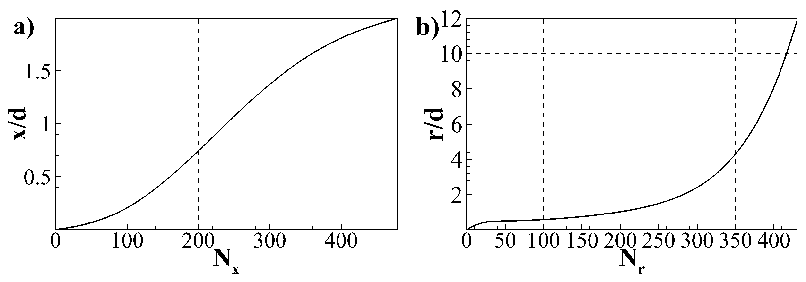
3. Numerical Methods

The compressible conservation equations of mass, momentum, and total energy in cylindrical coordinates are the governing equations. These equations are non-dimensionalised with respect to the ambient conditions. The filtered equations for the LES model are derived by introducing a spatial convolution defined as

$$\overline{\varphi }(\mathbf{x},\mathbf{t})=\int \int {\int }_{{\mathbb{R}}^{\mathbf{3}}}\mathbf{G}(\frac{\mathbf{x}-\zeta }{\Delta })\varphi (\zeta ,\mathbf{t})\mathbf{d}\zeta ,$$

(2)

where G is the filter function, $\Delta$ the cut-off spatial scale, $\varphi (\zeta ,t)$ an unfiltered variable, and $\overline{\varphi }(\mathbf{x},\mathbf{t})$ a filtered variable. The filter decomposes the flow field into a resolvable field, $\overline{\varphi }$, and a subgrid-scale (SGS) field, ${\varphi }^{″}$, as

$$\begin{array}{c}\hfill \varphi =\overline{\varphi }+{\varphi }^{″}.\end{array}$$

(3)

The Favre filtering operator, defined as $\overline{\rho \varphi }=\overline{\rho }\tilde{\varphi }$, is used to avoid the subgrid terms arising in the continuity equation. Applying this filtering, the filtered Navier–Stokes equations are expressed as:

$$\begin{array}{ccc}\hfill \frac{\partial \overline{\rho }}{\partial t}& \hfill +& \nabla ·\left(\overline{\rho }\tilde{\mathbf{u}}\right)=0,\hfill \\ \hfill \frac{\partial \overline{\rho }\tilde{\mathbf{u}}}{\partial t}& \hfill +& \nabla ·(\overline{\rho }\tilde{\mathbf{u}}\otimes \tilde{\mathbf{u}}+\overline{p}\mathbb{I}-\tilde{\mu }\tilde{\mathbb{T}})=\nabla ·({\mathbb{F}}_R+{\mathbb{F}}_{VM}),\hfill \\ \hfill \frac{\partial \overline{\rho }\tilde{e}}{\partial t}& \hfill +& \nabla ·\left[\tilde{\mathbf{u}}(\overline{\rho }\tilde{e}+\overline{p})-\tilde{k}\nabla \tilde{T}-\tilde{\mu }\tilde{\mathbb{T}}·\tilde{\mathbf{u}}\right]=\nabla ·({\mathbb{F}}_E+{\mathbb{F}}_{VT}+{\mathbb{F}}_{VE}).\hfill \end{array}$$

(4)

The terms appearing on the right-hand-side of the equations are subgrid-scale terms which need closure models. The filtered deviatoric stress tensor, $\tilde{\mathbb{T}}$, and thermal conductivity, $\tilde{k}$, are defined as:

$$\begin{array}{ccc}\hfill \tilde{\mathbb{T}}& \hfill =& \left[\nabla \tilde{\mathbf{u}}+{\left(\nabla \tilde{\mathbf{u}}\right)}^T+\left(\frac{{\mu }_b}{\tilde{\mu }}-\frac{2}{3}\right)(\nabla ·\tilde{\mathbf{u}})\mathbb{I}\right],\hfill \\ \hfill \tilde{k}& \hfill =& \tilde{\mu }\frac{\gamma }{\gamma -1}\frac{1}{M_o^{2}Pr}.\hfill \end{array}$$

(5)

The other relevant equations are the filtered equation of state, $\overline{p}=\overline{\rho }\tilde{T}/M_o^2$, and the filtered sensible internal energy which results in a subgrid turbulent kinetic energy, $K_s$, as:

$$\begin{array}{c}\hfill \frac{1}{2}{K}_s=\overline{\rho }\tilde{e}-\frac{1}{2}\overline{\rho }\tilde{\mathbf{u}}·\tilde{\mathbf{u}}-\frac{\overline{\rho }\tilde{T}}{M_o^2(\gamma -1)}=\overline{\rho }\tilde{e}-\frac{1}{2}\overline{\rho }\tilde{\mathbf{u}}·\tilde{\mathbf{u}}-\frac{\overline{p}}{(\gamma -1)}.\end{array}$$

(6)

The subgrid viscous terms (${\mathbb{F}}_{VT}$, ${\mathbb{F}}_{VE}$, and ${\mathbb{F}}_{VM}$) are contributions of subgrid viscosity, ${\mu }^{″}$, and are assumed to be negligible. The subgrid Reynolds stress, ${\mathbb{F}}_R$, and subgrid turbulent kinetic energy, $K_s$, are computed using Germano’s dynamic model with the adjustment of Lilly [27]. The subgrid internal energy mixing, ${\mathbb{F}}_E$, is evaluated using an eddy-diffusivity model [28].

The model developed by Mohseni and Colonius [29] is used for the treatment of the centreline numerical singularity in cylindrical coordinates. In this method, the first radial grid point is located at $\Delta r/2$ and a transformation is required for the radial coordinate where any scalar and vector quantities of the radial axis change sign when their azimuthal location is more than $\pi$. This approach has been used in different studies, as it is accurate and simple to implement [5,30]. In addition, an eleven-point stencil filter is required to suppress numerical fluctuations at the centreline.

No treatment is required for the supersonic inlet boundary condition, as there is no outward propagation wave. The flow at the outlet boundaries is considered to be subsonic flow. Therefore, non-reflecting outflow boundary conditions are imposed on these boundaries [31,32]. In addition, the optimised sponge region of Mani [33] is employed near the outflow boundaries to minimise the reflections from the outflow boundaries. In the sponge regions, the flow field is forced to a self-similar solution, which was determined a priori.

In the supersonic impinging jet, the normal pressure gradient at the wall is high and the local one-dimensional inviscid relation conflicted with the physical condition on the wall [34]. Therefore, the modified Navier–Stokes equations are considered on the boundaries rather than the characteristic equations in our implementation of the wall boundary condition. There are no convective terms, as the no-slip wall boundary condition is assumed. The wall is located at a midpoint distance after the last computational grid point. For the sixth-order spatial discretisation applied here, four extra cell points are used as ghost cells where the primitive variables are evaluated using the Taylor extrapolation for these points. These ghost cells are used to evaluate declivities at the boundaries.

A sixth-order central finite difference method is applied in the smooth regions in the spatial directions, while a fifth-order weighted essentially non-oscillating (WENO) scheme with local Lax–Friedrichs flux splitting is used in the discontinuous regions. This hybrid approach relies on a sensor to determine in which regions the WENO scheme must be used. A commonly used shock sensor is that proposed by Ducros et al. [35]. In this model, the shock sensor $\Psi$ is expressed as:

$$\begin{array}{c}\hfill {\Psi }_i=\left|\frac{p_{i+1}-2p_i+p_{i-1}}{p_{i+1}+2p_i+p_{i-1}}\right|\frac{{(\nabla ·\mathbf{u})}^2}{{(\nabla ·\mathbf{u})}^2+{\omega }^2+{ϵ}_0},\end{array}$$

(7)

where $\omega$ is vorticity and $ϵ={10}^{-30}$ was chosen to prevent numerical divergence in the region where the flow is free of dilatation and vorticity. In addition, a threshold $\sigma$ is needed to switch the WENO scheme on and off. Lo et al. [36] used a single value of 0.01 (i.e., the WENO scheme is active if ${\Psi }_i>0.01$) in their study. Another expression for the shock sensor was proposed by Larsson et al. [37] in the hybrid WENO/central scheme as:

$$\begin{array}{c}\hfill {\Psi }_i=\frac{-\nabla ·\mathbf{u}}{\nabla ·\mathbf{u}+\sqrt{{\omega }^2}},\end{array}$$

(8)

with the WENO method being active in regions where ${\Psi }_i>0.65$.

These techniques detect shock/discontinuity effectively. However, they also consider high-frequency fluctuations and critical points as shocks. In our LES simulations, it was observed that this shock sensor performed poorly by activating the WENO scheme in the entire shear layer of the jet. Therefore, a new definition for the shock sensor was developed. The new shock sensor definition is based on the smoothness definition in the WENO scheme. The most right and left smoothness parameters $I{S}_0^{+}$ and $I{S}_0^{-}$ are used to define a new indicator ${\beta }_q$ as:

$$\begin{array}{c}\hfill {\beta }_q=|I{S}_0^{+}\left(q\right)-I{S}_0^{-}\left(q\right)|,\end{array}$$

(9)

where the pressure and density are considered as the primitive variables to define the sensor. The WENO scheme is active in the region where this indicator for any of pressure or density exceeded a threshold value of ${\sigma }_q$, which depends on the numerical grid size. In this study, the expression for linear scaling with the grid size of $C_{ss}d{x}_i$ is found as an optimal criterion, where $C_{ss}$ is a model constant.

The temporal integration is performed using a fourth-order five-step Runge–Kutta scheme [38,39].

The in-house-developed high-fidelity LES parallel code that implements this numerical algorithm has been tested and validated in previous studies [9,11,40,41,42], and is used in this study to solve the spatially filtered Navier–Stokes equations with appropriate boundary conditions.

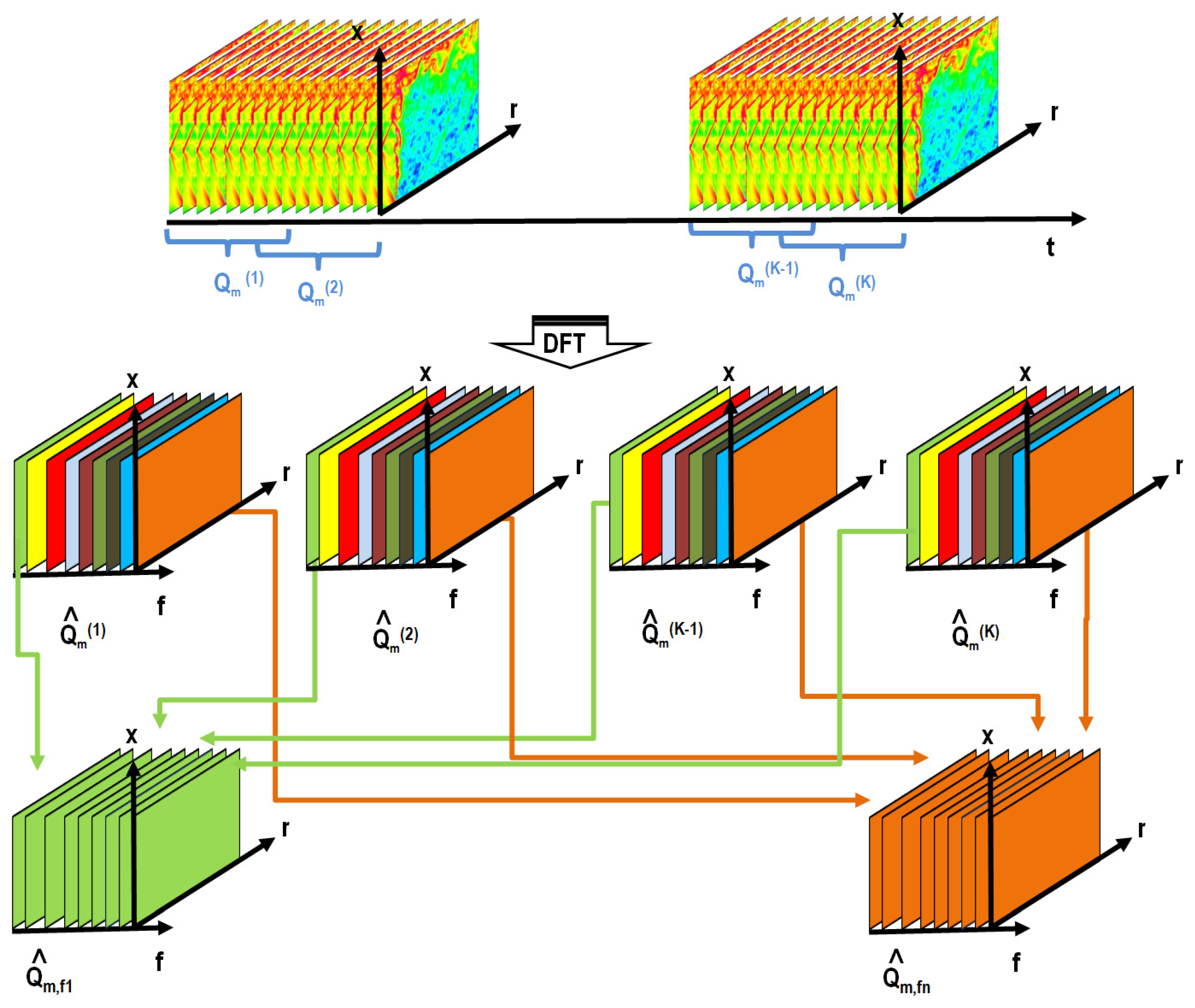
4. Spectral Proper Orthogonal Decomposition (SPOD)

Spectral proper orthogonal decomposition (SPOD) was first introduced by Lumley [22]. This decomposition method identifies energy-ranked modes where each oscillates at a single frequency, and has been overlooked since its inception despite its benefits over the common spatial form of POD [43] and dynamic mode decomposition [16]. There are few techniques in the literature for computing SPOD modes [13,44,45]. In this study, we used the procedure developed by Towne et al. [13], as it was found to be computationally more efficient compared to others. The details of the procedure can be found in the comprehensive paper by Towne et al. [13]. However, the algorithm is outlined here for the sake of completeness.

Consider a vector $\mathbf{q}$, which contains the three-dimensional spatial distribution of the flow variables at instance $t_k$. In the configuration of this study, the flow is homogeneous with respect to the azimuthal direction. Therefore, it can be decomposed into azimuthal Fourier modes (${\widehat{\mathbf{q}}}_m$). If we assume that the flow field is available for M time instants which are equally spaced, then the dataset can be organised in a compact matrix form of

$${\widehat{\mathbf{Q}}}_m=[{\widehat{\mathbf{q}}}_{1,m},{\widehat{\mathbf{q}}}_{2,m},...,{\widehat{\mathbf{q}}}_{M,m}],$$

(10)

which has $N\times M$ dimension where N is the number of spatial points (radial and axial) times the number of variables. The converged estimation of the cross-spectral density tensor can be obtained by averaging the spectra over multiple realizations of the flow using Welch’s method. Therefore, the dataset is partitioned into smaller overlapping blocks, each of which represents an ensemble realization of the flow. These blocks are shown schematically in Figure 3 by ${\mathbf{Q}}_m^{\left(b\right)}$. A temporal discrete Fourier transform of each block is then calculated, ${\widehat{\mathbf{Q}}}_m^{\left(b\right)}$. To reduce spectral leakage, a Hanning window is used to reduce the discontinuities with a hypothetical next period. A new data matrix is formed at the k-th frequency by collecting all of the Fourier realizations of the blocks ${\widehat{\mathbf{Q}}}_{(m,f_k)}$. This is shown in Figure 3 using the same colour rectangular shapes. This yields the estimated cross-spectral density tensor at frequency $f_k$ as:

$${\widehat{\mathbf{S}}}_{(m,f_k)}={\widehat{\mathbf{Q}}}_{(m,f_k)}{\widehat{\mathbf{Q}}}_{(m,f_k)}^{*}.$$

(11)

For the particular frequency, the SPOD modes are found as the eigenvectors ${\mathbf{\Psi }}_{\mathbf{m},{\mathbf{f}}_{\mathbf{k}}}=\left[{\psi }_{m,f_k}^{\left(1\right)}{\psi }_{m,f_k}^{\left(2\right)}...{\psi }_{m,f_k}^{\left(n_b\right)}\right]$, and the total energy as the corresponding eigenvalues ${\mathbf{\Lambda }}_{\mathbf{m},{\mathbf{f}}_{\mathbf{k}}}=diag\left({\lambda }_{m,f_1}^{\left(1\right)}{\lambda }_{m,f_2}^{\left(2\right)}...{\lambda }_{m,f_{n_f}}^{\left(n_b\right)}\right)$ of the weighted cross-spectral density matrix ${\widehat{\mathbf{S}}}_{(m,f_k)}$ as

$${\widehat{\mathbf{S}}}_{(m,f_k)}\mathbf{W}{\mathbf{\Psi }}_{\mathbf{m},{\mathbf{f}}_{\mathbf{k}}}={\mathbf{\Psi }}_{\mathbf{m},{\mathbf{f}}_{\mathbf{k}}}{\mathbf{\Lambda }}_{\mathbf{m},{\mathbf{f}}_{\mathbf{k}}}.$$

(12)

The eigenvalues are ordered from the largest to smallest. The eigenvector corresponding to the largest eigenvalue is the leading or optimal mode, and the subsequent smaller eigenvalues (i.e., lower-energy modes) are suboptimal modes at each azimuthal mode number. The total energy, $E_t$, of the flow can be obtained by summation over all of the eigenvalues as:

$$E_t=\sum _{m=0}^{n_m}\sum _{k=0}^{n_f}\sum _{i=0}^{n_b}{\lambda }_{m,f_k}^{\left(i\right)}.$$

(13)

5. Results

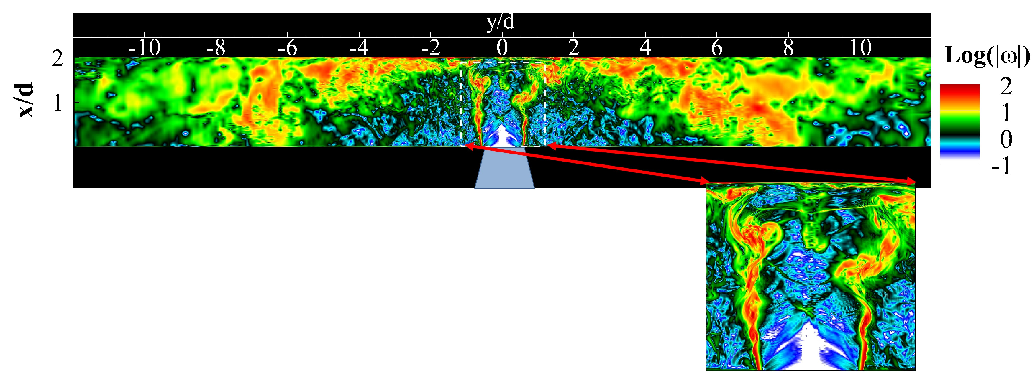
5.1. Characteristics of the Flow-Field

The first- and second-order statistics of the flow field are presented in this section. Before we discuss the characteristic of the flow, to validate the present LES, the comparison of the mean streamwise velocity field (a) and twice of streamwise turbulent kinetic energy (b) with the experimental results of Weightman et al. [21] are presented in Figure 4. With the caveat that the experimental results are for the Reynolds number of 680,000 (an order of magnitude higher than the condition of this simulation), the results are in good agreement with the experiment. The slight difference in the location of the Mach disk is considered to be due to the difference in the Reynolds number, and also the sensitivity of the mean field to inlet conditions as recently investigated by Markesteijn et al. [46].

Now moving to the discussion of the first- and second-order statistics of the flow field, contour maps of ensemble-averaged streamwise and radial velocities, as well as pressure obtained from LES are shown in Figure 5. Figure 5a shows the mean streamwise velocity with streamlines near the nozzle exit and impingement region magnified in the rectangular sub-frames. The initial expansion of the shear layer upon exiting from the nozzle is clearly visible. There is a high level of entrainment near the nozzle at the region marked by “A” as visualised by streamlines in the zoomed sub-frame. The velocity vectors are directed perpendicularly towards the jet except very close to the nozzle lip where they move towards the nozzle and then into the jet due to the infinite lip and the no-slip boundary condition. A small Mach disk with a size of 0.1d is also observed at $x/d\approx$ 1.0 (marked with a “B”). The small size of the Mach disk is due to the low NPR of 3.4 [47]. Other classical features of supersonic flow, like a triple point and an oblique shock, are also visible. Upon the impingement, a recirculation bubble is formed (labelled as “C”) and streamlines of the flow field highlight this phenomenon more precisely. Figure 5b shows the radial velocity contour. The triple point and oblique shock are easy to perceive in this plot. The negative mean radial velocity in the region outside of the jet confirms the entrainment. The formation of a strong wall jet at the impinging wall after the recirculation zone is evident. The mean pressure field is presented in Figure 5c. There is an excessive pressure drop before the Mach disk. There is also a high-pressure region in the impingement zone as a stagnation occurrs and a stand-off shock is formed. A streamwise modulation in all three variables is observed, similar to the modulations reported in previous experimental and numerical studies [4,5,6,12,20,48,49,50,51].

The second-order statistics are also examined. Contour maps of the mean streamwise density-weighted Reynolds stress are presented in Figure 6a, the mean radial density-weighted Reynolds stress in Figure 6b, and the mean shear stress in the streamwise-radial plane in Figure 6c. The black line is the maximum radial location of the turbulent kinetic energy within the shear layer. The Reynolds stresses have high positive values in the shear layer which is expected and they contribute to the turbulence generation. There are also local maxima at the Mach disk (triple point), stand-off shock, and the impinging wall. All three components show small variations at the oblique shock. The mean streamwise density-weighted Reynolds stress is intense in the Mach disk, while the radial component is intense close to the impinging wall. This highlights the high turbulence level in the stagnation bubble, which is also found in the vorticity field (Figure 2).

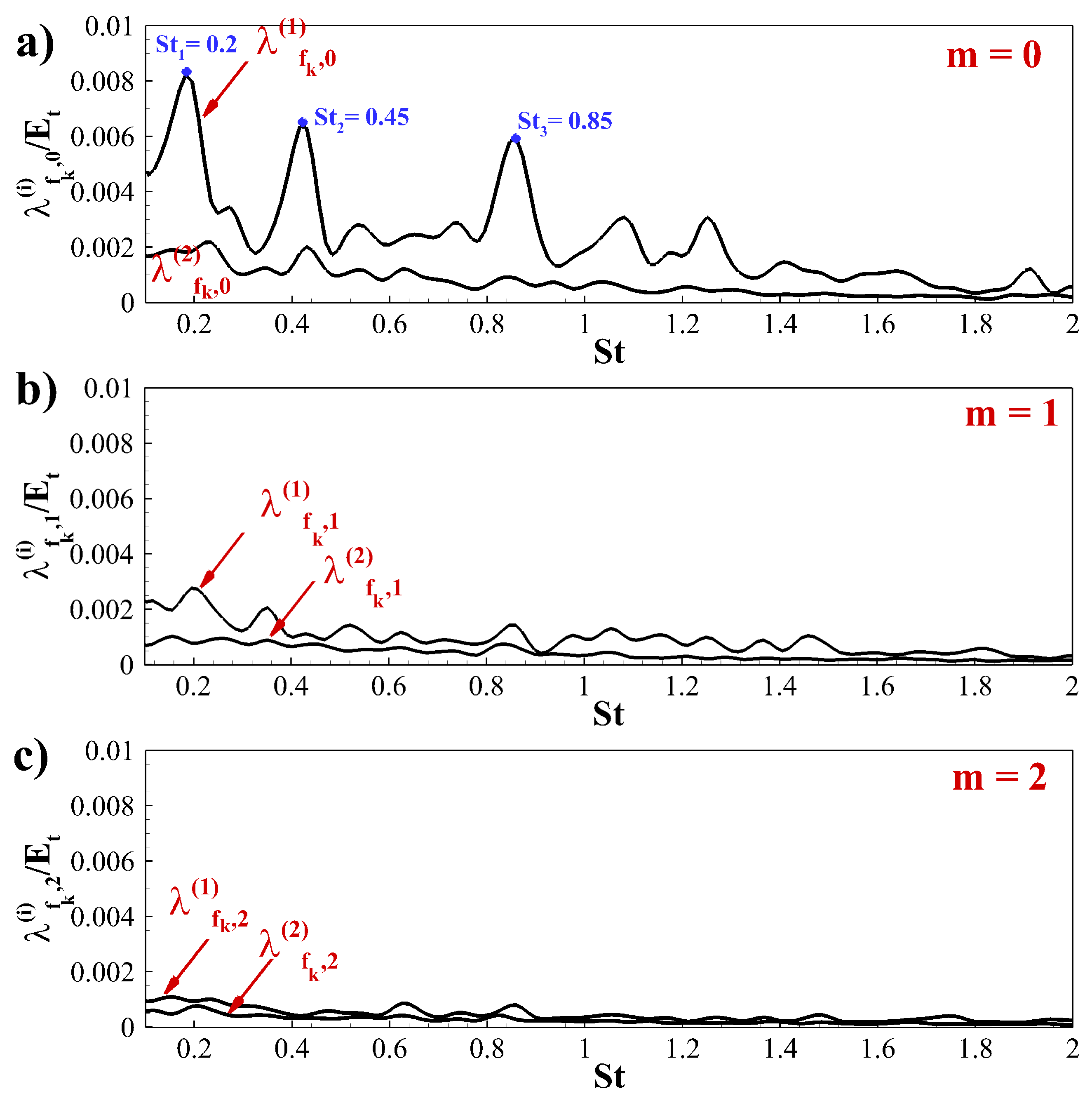
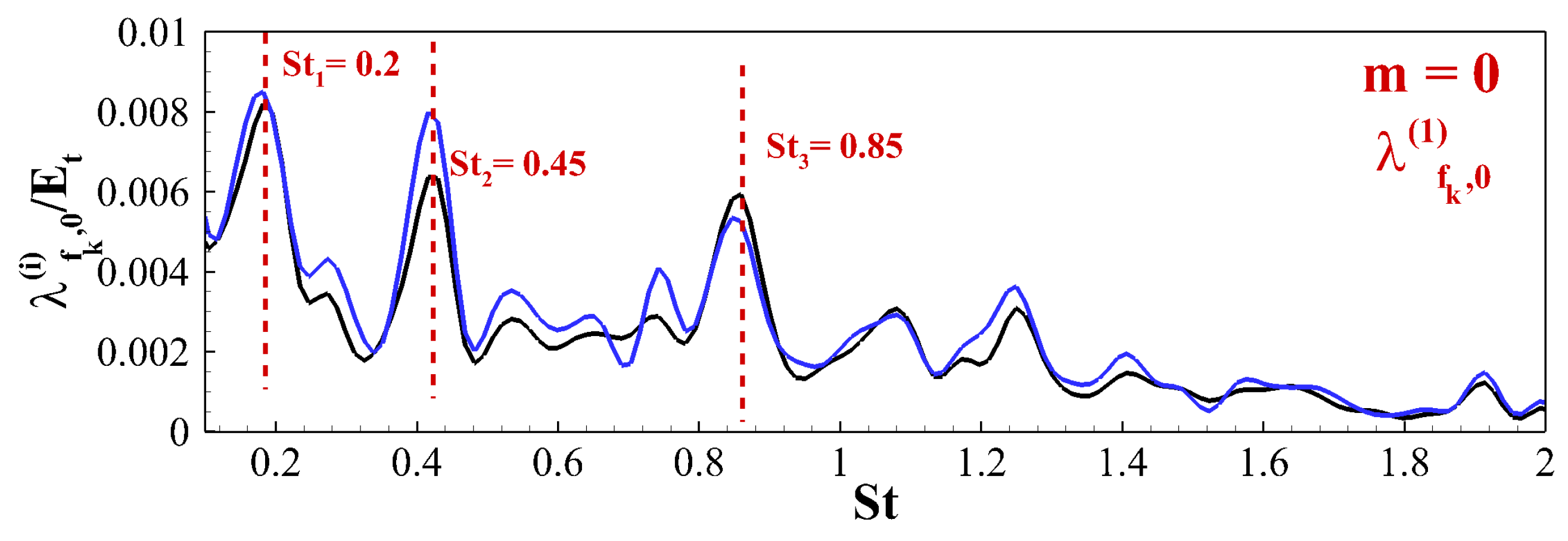
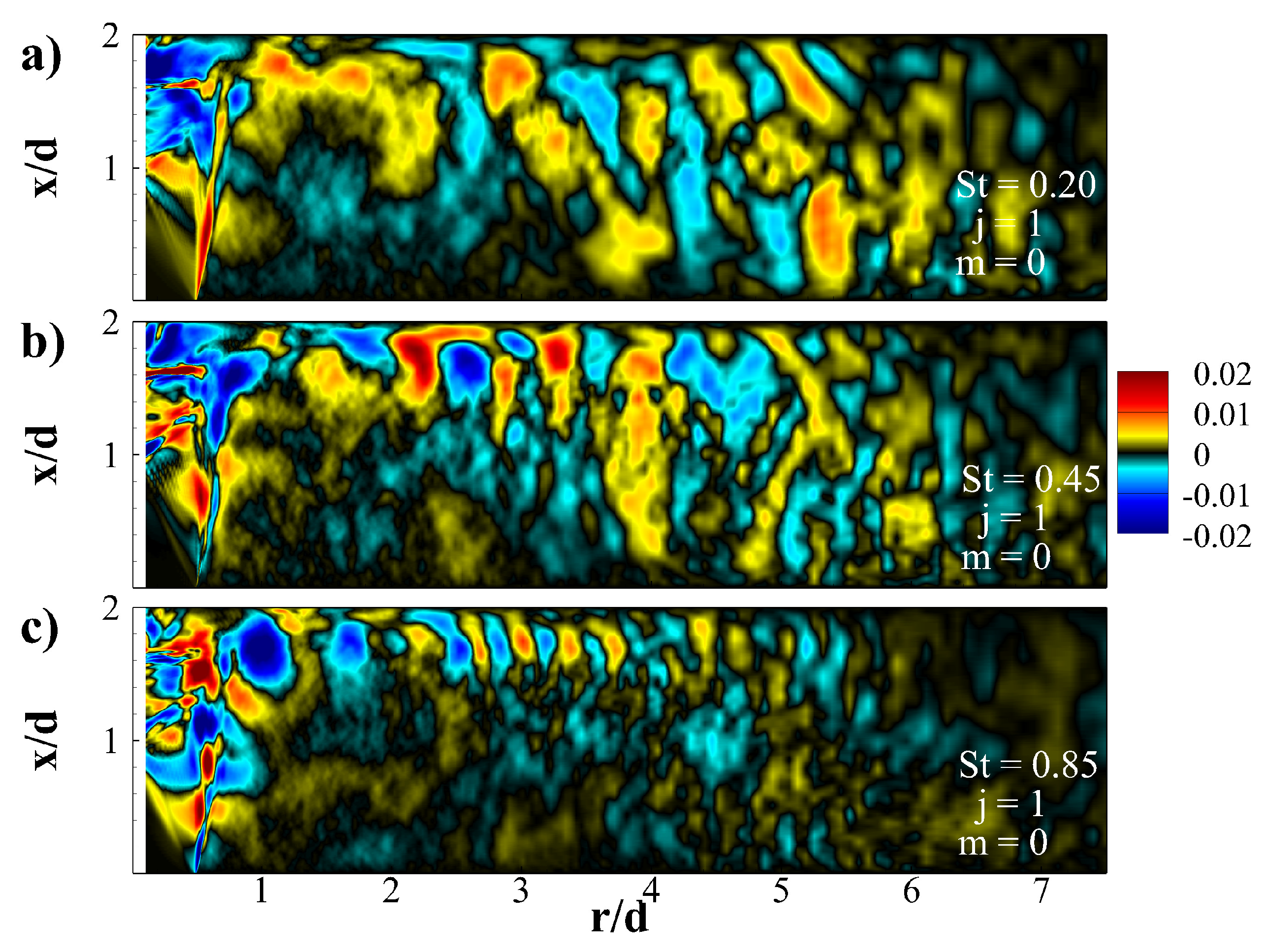
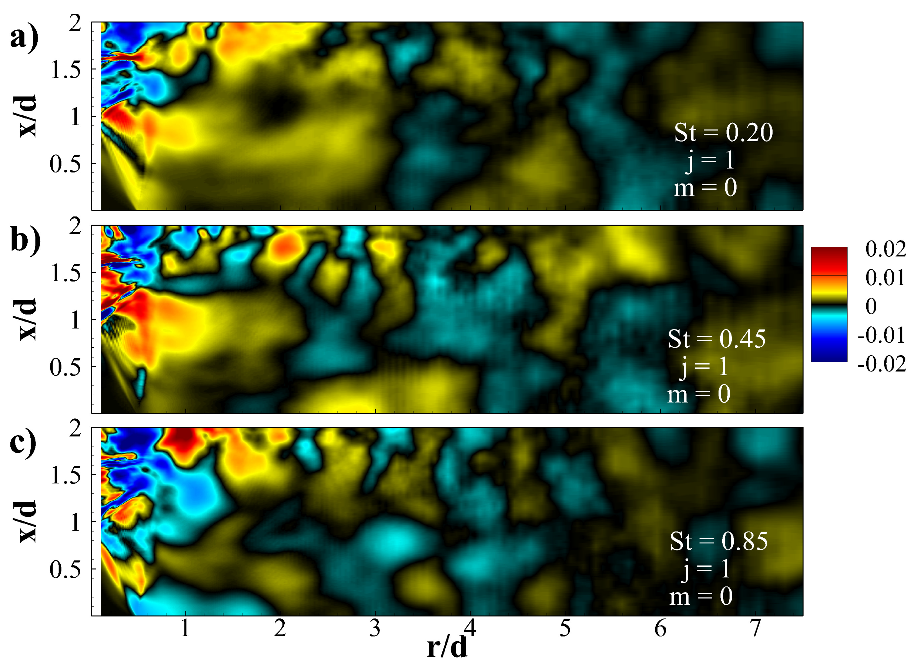
5.2. Spectral Proper Orthogonal Decomposition (SPOD) Modes

SPOD modes are obtained by applying the formulation developed by Towne et al. [13] and briefly outlined in Section 4 to the time-resolved three-dimensional flow field obtained from a large eddy simulation. The LES dataset consists of 4000 three-dimensional snapshots collected every 0.05 acoustic time units. There are 512 snapshots in each block, with an overlap of 348 snapshots with a standard Hanning window to reduce the spectral leakage. This yields 26 blocks or realizations of the flow (this is interpreted as performing an experiment of the same problem 26 times at the same conditions and for a time period of 25.6 acoustic time units). The combination of 512 sequential snapshots with the 348 overlapped snapshots was found to be sufficient to capture coherent structures in this configuration. Note that the sensitivity of the findings to a higher frequency resolution by increasing the period to 51.2 acoustic time units, a higher overlapping of 448 snapshots, and a lower overlapping of 256 snapshots was performed, and no effect on the results in either the modes or the peaks in the spectra was observed. The other parameters are the domain of interest and primitive variables which vary depending on the research question. Different primitive variables have been used in previous studies of jet flows [13,17,45,52]. We used the entire domain of the large eddy simulation (i.e., $0<x/d<2$ and $0<r/d<12$) with the primitive variables of pressure, three components of the velocity vector and density. Figure 7 shows the accumulative energy for each azimuthal mode obtained from SPOD decomposition, where the energy of each azimuthal mode is obtained by summation of energy over all temporal frequencies and blocks (see Equation (13)). The first three azimuthal modes contains more than $60\%$ of the total energy. The leading azimuthal mode is the axisymmetric mode ($m=0$) which contained $34\%$ of the total energy, followed by azimuthal mode numbers 1 and 2 with $20\%$ and $12\%$ of total energy, respectively. Therefore, for the rest of the paper, only the first three azimuthal modes are considered, and the other azimuthal modes are omitted from the subsequent analysis.

The spectrum of the SPOD eigenvalues normalised by total flow energy as a function of Strouhal number for the first and second SPOD modes of the first three azimuthal mode numbers of (a) $m=0$ (axisymmetric), (b) $m=1$ (helical), and (c) $m=2$ are shown in Figure 8. y-axes show the normalised eigenvalues, and they have the same scaling in all subplots to facilitate the discussion. The first axisymmetric mode appears as the optimal mode with three dominant peaks in the frequency domain. A large separation between the optimal mode and the second mode is clear in the axisymmetric mode and therefore the flow exhibits a low-rank behaviour. This low-rank behaviour of the flow has a discrete frequency nature. The three dominant Strouhal numbers are 0.20, 0.45, and 0.85. Before presenting the spatial distribution of these dominant features of the flow, it is necessary to examine the convergence of the computed modes. Therefore, 75% of the dataset is used with a combination of 512 sequential snapshots with 348 overlapped to compute the spectrum. The results for the first axisymmetric mode are presented in Figure 9 using the 100% and 75% percent of the dataset to perform SPOD analysis. It is clear from this figure that the time period of LES dataset is long enough to recover the dominant structures in this configuration.

Figure 10 shows the spatial field of streamwise velocity for these Strouhal numbers. Very complex interactions of spatial wavepackets emerge in all three Strouhal numbers. The wavepackets in the shear layer of the jet are connected to the structures formed at the Mach disk and the stand-off shock. There are no wavepackets in the conical region of the jet, as the flow was supersonic. For the first two Strouhal numbers, the high amplitude structures are inside the jet close to the Mach disk and the stand-off shock, as well as in the shear layer. Upon the impingement, these structures are disconnected and a separated region is formed in the wall jet. The behaviour is slightly different for high Strouhal numbers. The high-amplitude wave packets are in the shear layer of the jet and developed into wave packets in the wall jet. The wavelengths of these wave packets grow as convected in the shear layer and maximise as impinging on the wall and decay as convected in the wall jet. In all three Strouhal numbers, there are weak structures in the region of $3<r/d<6$. The dominant frequencies of the optimal mode obtained from SPOD appear to have similar spatial structures to the most energetic (POD) modes of the under-expanded jets of Weightman et al. [51]. However, the advantage of the analysis in the present study is that it reveals the Strouhal numbers (i.e., frequencies) of these spatial modes which were not directly available from POD. It is noted that POD modes are contributions from many SPOD modes at different frequencies [13]. It is commonly assumed that the expansion coefficients are uncorrelated at different times, and therefore that the frequency contents of the modes are available from these expansion coefficients. However, this assumption is not valid [13].

The two high frequencies obtained by SPOD appear as sub-harmonics of the fundamental frequency. The interaction between a wave and its sub-harmonic in free jets and shear layer produces a sub-harmonic component. This sub-harmonic component may excite the jet depending on its phase, and initiates a subharmonic resonance [53]. The subharmonic growth in the shear layer and vortex pairing depends on the phase difference [54]. If there is no external excitation, the random jitter in the pairing location prevents the periodic pairings and results in a broadband spectrum. However, in this under-expanded supersonic impinging jet, the complex interactions of vortex-oblique shock and vortex-wall impose acoustic forces on the system, which does not exist in free subsonic round jets and subsonic impinging jets with no external excitation. The effect of external excitations on the flow structure of a subsonic impinging jet with Reynolds number of 10,000 was studied experimentally by Vejrazka et al. [55]. The results showed that the jet was sensitive to simultaneous excitation at two frequencies: fundamental and its sub-harmonic. This simultaneous excitation results in variations in size, strength, and convection velocity of the individual vortices, which is consistent with the observation of complex structures in this study.

The near-field acoustic structures of these Strouhal numbers are considered now. The spatial pressure fields of the axisymmetric azimuthal mode for different Strouhal numbers of (a) $St=0.20$, (b) 0.45, and (c) 0.85 are presented in Figure 11. The pressure contour maps show a very complex behaviour in the region confined by the shear layer, Mach disk, and the impinging wall. This complexity makes the physical interpretation of the behaviour in this region difficult. However, the high level of fluctuations in this region shows the dominant roles of the Mach disk, the shock waves, and the flow–wall interaction in this flow configuration. Moving to the near-field pressure outside of the jet, there are footprints of the waves initiated at the impingement or in the wall jet. There are also signs of strong pressure waves near the nozzle lip. There is just one caveat, that the pressure field inside of the plume of the jet does not have a pure acoustic nature. However, in the under-expanded jet of this study, the supersonic line which forms a cone prevents any acoustic waves from reaching the nozzle lip, and the only mechanism by which acoustic waves can reach the nozzle lip is propagation in outside of this region.

These simultaneous observations of the spatial distribution of hydrodynamic wave packets in the shear layer and the impingement and acoustic waves in the near field of the jet and specifically at the impinging region and close to the nozzle lip confirm the presence of some form of feedback loop in each frequency for the optimal mode. To further elaborate on the feedback loop, the cross-spectrum density of the streamwise velocity fluctuations at the nozzle lip and near-field pressure is examined. The pressure fluctuations are sampled at locations on an arch with a radius of 1d as shown schematically in Figure 12. Note that the vorticity is negligible in these locations, as can be seen in Figure 2a, where the logarithm of vorticity magnitude is presented. Therefore, pressures at these sampling locations are assumed to have acoustic nature with a good approximation. The cross-spectrum density of the streamwise velocity fluctuations near the nozzle lip and the near-field pressure fluctuations at sample points is shown in Figure 12b. There is a high cross-spectrum density of the velocity fluctuations, and the near-field pressure fluctuations at the dominant frequencies obtained from SPOD decomposition, which further clarifies the presence of a feedback loop.

6. Conclusions

The spectral proper orthogonal technique is used to study coherent structures in an under-expanded supersonic impinging jet. A time-resolved LES of an under-expanded supersonic impinging jet is first performed. The first- and second-order statistics of the flow field are presented. The accumulative energy obtained from SPOD in each azimuthal mode show that the first three azimuthal modes contain more than 60% of the total energy. However, the spectra show that the axisymmetric mode is the leading mode. SPOD reveals that the flow has a low-ranked behaviour and the first azimuthal mode is the optimal mode. There are also dominant discrete frequencies in this optimal mode which has Strouhal numbers of 0.2, 0.45, and 0.85. The spatial fields of the streamwise velocity and the pressure of these discrete frequencies are presented. The complex interactions of the wave packets with oblique shocks, Mach disk, and stand-off shock are observed. The impingement also altered the wave packets, which is clearer when the wave packets of the jet were disconnected from the wall jet at low Strouhal number (i.e., $St=0.2$).

This analysis show that unlike the wave packets in the subsonic and supersonic free jets of Schmidt et al. [56], the wave packets are more complex and convoluted. They form a Kelvin–Helmholtz wave packet type in the shear layer of the jet and appear more evident at high Strouhal numbers. However, in contrast to free jets in the under-expanded supersonic impinging jet, they are connected to the Mach disk and stand-off shock.

The more striking result is the connection between the acoustic waves and shear layer instabilities. Both of these quantities show high amplitude for the optimal mode at dominant Strouhal numbers. The hydrodynamic instabilities are identified in the shear layer of the jet as Kelvin–Helmholtz wave packets and in the near-field of the jet as acoustic waves. The high amplitude of the pressure wave in the vicinity of the nozzle lip for each dominant frequency of the optimal mode show the connection between hydrodynamic and acoustic wave packets, which identified a feedback loop in each of these dominant frequencies of the optimal mode.

References

1. Raman, G.; Srinivasan, K. The powered resonance tube: From Hartmann’s discovery to current active flow control applications. Prog. Aerosp. Sci. 2009, 45, 97–123. [Google Scholar] [CrossRef]
2. Powell, A. The sound-producing oscillations of round underexpanded jets impinging on normal plates. J. Acoust. Soc. Am. 1988, 83, 515–533. [Google Scholar] [CrossRef]
3. Henderson, B.; Powell, A. Experiments concerning tones produced by an axisymmetric choked jet impinging on flat plates. J. Sound Vib. 1993, 168, 307–326. [Google Scholar] [CrossRef]
4. Mason-Smith, N.; Edgington-Mitchell, D.; Buchmann, N.A.; Honnery, D.R.; Soria, J. Shock structures and instabilities formed in an underexpanded jet impinging on to cylindrical sections. Shock Waves 2015, 25, 611–622. [Google Scholar] [CrossRef]
5. Gojon, R.; Bogey, C. Flow Structure Oscillations and Tone Production in Underexpanded Impinging Round Jets. AIAA J. 2017, 55, 1792–1805. [Google Scholar] [CrossRef]
6. Amili, O.; Edgington-Mitchell, D.; Honnery, D.; Soria, J. Interaction of a supersonic underexpanded jet with a flat plate. In Fluid-Structure-Sound Interactions and Control; Springer: Heidelberg/Berlin, Germany, 2016; pp. 247–251. [Google Scholar]
7. Mitchell, D.M.; Honnery, D.R.; Soria, J. The visualization of the acoustic feedback loop in impinging underexpanded supersonic jet flows using ultra-high frame rate schlieren. J. Vis. 2012, 15, 333–341. [Google Scholar] [CrossRef]
8. Gojon, R.; Bogey, C.; Marsden, O. Large-eddy simulation of underexpanded round jets impinging on a flat plate 4 to 9 radii downstream from the nozzle. In Proceedings of the 21st AIAA/CEAS Aeroacoustics Conference, AIAA Aviation Forum, Dallas, TX, USA, 22–26 June 2015; p. AIAA 2015-2210. [Google Scholar]
9. Stegeman, P.; Ooi, A.; Soria, J. Proper Orthogonal Decomposition and Dynamic Mode Decomposition of Under-Expanded Free-Jets with Varying Nozzle Pressure Ratios. In Instability and Control of Massively Separated Flows; Springer: Heidelberg/Berlin, Germany, 2015; pp. 85–90. [Google Scholar]
10. Edgington-Mitchell, D.; Oberleithner, K.; Honnery, D.R.; Soria, J. Coherent structure and sound production in the helical mode of a screeching axisymmetric jet. J. Fluid Mech. 2014, 748, 822–847. [Google Scholar] [CrossRef]
11. Karami, S.; Stegeman, P.C.; Theofilis, V.; Schmid, P.J.; Soria, J. Linearised dynamics and non-modal instability analysis of an impinging under-expanded supersonic jet. J. Phys. Conf. Ser. 2018, 1001, 012019. [Google Scholar] [CrossRef] [Green Version]
12. Henderson, B.; Bridges, J.; Wernet, M. An experimental study of the oscillatory flow structure of tone-producing supersonic impinging jets. J. Fluid Mech. 2005, 542, 115–137. [Google Scholar] [CrossRef]
13. Towne, A.; Schmidt, O.T.; Colonius, T. Spectral proper orthogonal decomposition and its relationship to dynamic mode decomposition and resolvent analysis. J. Fluid Mech. 2017, 825, 1113–1152. [Google Scholar] [CrossRef]
14. Schmid, P.J. Nonmodal stability theory. Annu. Rev. Fluid Mech. 2007, 39, 129–162. [Google Scholar] [CrossRef]
15. Bagheri, S.; Schlatter, P.; Schmid, P.J.; Henningson, D.S. Global stability of a jet in crossflow. J. Fluid Mech. 2009, 624, 33–44. [Google Scholar] [CrossRef]
16. Schmid, P.J. Dynamic mode decomposition of numerical and experimental data. J. Fluid Mech. 2010, 656, 5–28. [Google Scholar] [CrossRef] [Green Version]
17. Schmidt, O.T.; Towne, A.; Colonius, T.; Cavalieri, A.V.; Jordan, P.; Brès, G.A. Wavepackets and trapped acoustic modes in a turbulent jet: coherent structure eduction and global stability. J. Fluid Mech. 2017, 825, 1153–1181. [Google Scholar] [CrossRef]
18. Sieber, M.; Paschereit, C.O.; Oberleithner, K. Spectral proper orthogonal decomposition. J. Fluid Mech. 2016, 792, 798–828. [Google Scholar] [CrossRef] [Green Version]
19. Bogey, C.; Gojon, R. Feedback loop and upwind-propagating waves in ideally expanded supersonic impinging round jets. J. Fluid Mech. 2017, 823, 562–591. [Google Scholar] [CrossRef] [Green Version]
20. Krothapalli, A.; Rajkuperan, E.; Alvi, F.; Lourenco, L. Flow field and noise characteristics of a supersonic impinging jet. In Proceedings of the 4th AIAA/CEAS Aeroacoustics Conference, Toulouse, France, 2–4 June 1998; p. 2239. [Google Scholar]
21. Weightman, J.L.; Amili, O.; Honnery, D.; Edgington-Mitchell, D.; Soria, J. On the Effects of Nozzle Lip Thickness on the Azimuthal Mode Selection of a Supersonic Impinging Flow. In Proceedings of the 23rd AIAA/CEAS Aeroacoustics Conference, Denver, CO, USA, 5–9 June 2017; p. AIAA 2017-3031. [Google Scholar]
22. Lumley, J.L. Stochastic Tools in Turbulence; Dover Publications: Mineola, NY, USA, 2007. [Google Scholar]
23. Glauser, M.N.; Leib, S.J.; George, W.K. Coherent structures in the axisymmetric turbulent jet mixing layer. In Turbulent Shear Flows 5; Springer: Heidelberg/Berlin, Germany, 1987; pp. 134–145. [Google Scholar]
24. Delville, J.; Ukeiley, L.; Cordier, L.; Bonnet, J.; Glauser, M. Examination of large-scale structures in a turbulent plane mixing layer. Part 1. Proper orthogonal decomposition. J. Fluid Mech. 1999, 391, 91–122. [Google Scholar] [CrossRef]
25. Bodony, D.J.; Lele, S.K. On using large-eddy simulation for the prediction of noise from cold and heated turbulent jets. Phys. Fluids 2005, 17, 085103. [Google Scholar] [CrossRef]
26. Kawai, S.; Lele, S.K. Large-eddy simulation of jet mixing in supersonic crossflows. AIAA J. 2010, 48, 2063–2083. [Google Scholar] [CrossRef]
27. Lilly, D.K. A proposed modification of the Germano subgrid-scale closure method. Phys. Fluids A Fluid Dyn. 1992, 4, 633–635. [Google Scholar] [CrossRef]
28. Martin, M.P.; Piomelli, U.; Candler, G.V. Subgrid-scale models for compressible Large Eddy Simulations. Theor. Comput. Fluid Dyn. 2000, 13, 361–376. [Google Scholar]
29. Mohseni, K.; Colonius, T. Numerical treatment of polar coordinate singularities. J. Comput. Phys. 2000, 157, 787–795. [Google Scholar] [CrossRef]
30. Bogey, C.; Marsden, O.; Bailly, C. Large-eddy simulation of the flow and acoustic fields of a Reynolds number 105 subsonic jet with tripped exit boundary layers. Phys. Fluids 2011, 23, 035104. [Google Scholar] [CrossRef]
31. Poinsot, T.; Lele, S.K. Boundary conditions for direct simulations of compressible viscous flows. J. Comput. Phys. 1992, 101, 104–129. [Google Scholar] [CrossRef]
32. Karami, S.; Hawkes, E.R.; Talei, M.; Chen, J.H. Stabilisation mechanisms in a turbulent lifted slot-jet flame at a low lifted height. J. Fluid Mech. 2015, 777, 633–689. [Google Scholar] [CrossRef]
33. Mani, A. Analysis and optimization of numerical sponge layers as a nonreflective boundary treatment. J. Comput. Phys. 2012, 231, 704–716. [Google Scholar] [CrossRef]
34. Liu, J.; Kaplan, C.R.; Oran, E.S. A Brief Note on Implementing Boundary Conditions at a Solid Wall Using the FCT Algorithm; Technical Report; Naval Research Lab: Washington, DC, USA, 2006. [Google Scholar]
35. Ducros, F.; Ferrand, V.; Nicoud, F.; Weber, C.; Darracq, D.; Gacherieu, C.; Poinsot, T. Large-eddy simulation of the shock/turbulence interaction. J. Comput. Phys. 1999, 152, 517–549. [Google Scholar] [CrossRef]
36. Lo, S.C.; Aikens, K.; Blaisdell, G.; Lyrintzis, A. Numerical investigation of 3-D supersonic jet flows using large-eddy simulation. Int. J. Aeroacoust. 2012, 11, 783–812. [Google Scholar] [CrossRef]
37. Larsson, J.; Lele, S.; Moin, P. Effect of Numerical Dissipation on the Predicted Spectra For Compressible Turbulence; Annual Research Briefs 2007; Center for Turbulence Research: Stanford, CA, USA, 2007; pp. 47–57. [Google Scholar]
38. Kennedy, C.A.; Carpenter, M.H. Several new numerical methods for compressible shear-layer simulations. Appl. Numer. Math. 1994, 14, 397–433. [Google Scholar] [CrossRef]
39. Kennedy, C.A.; Carpenter, M.H.; Lewis, R.M. Low-storage, explicit Runge–Kutta schemes for the compressible Navier–Stokes equations. Appl. Numer. Math. 2000, 35, 177–219. [Google Scholar] [CrossRef] [Green Version]
40. Stegeman, P.C.; Pérez, J.M.; Soria, J.; Theofilis, V. Inception and evolution of coherent structures in under-expanded supersonic jets. J. Phys. Conf. Ser. 2016, 708, 012015. [Google Scholar] [CrossRef]
41. Stegeman, P.C.; Soria, J.; Ooi, A. Interaction of Shear Layer Coherent Structures and the Stand-Off Shock of an Under-Expanded Circular Impinging Jet. In Fluid-Structure-Sound Interactions and Control; Springer: Heidelberg/Berlin, Germany, 2016; pp. 241–245. [Google Scholar]
42. Stegeman, P.; Soria, J.; Ooi, A. Dynamic Mode Decomposition of Near Nozzle Instabilities in Large-Eddy Simulations of Under-Expanded Circular Jets. In Proceedings of the 19th Australasian Fluid Mechanics Conference, Melbourne, Australia, 8–11 December 2014. [Google Scholar]
43. Sirovich, L. Turbulence and the dynamics of coherent structures. I. Coherent structures. Quart. Appl. Math. 1987, 45, 561–571. [Google Scholar] [CrossRef] [Green Version]
44. Gordeyev, S.V.; Thomas, F.O. Coherent structure in the turbulent planar jet. Part 1. Extraction of proper orthogonal decomposition eigenmodes and their self-similarity. J. Fluid Mech. 2000, 414, 145–194. [Google Scholar] [CrossRef]
45. Citriniti, J.; George, W.K. Reconstruction of the global velocity field in the axisymmetric mixing layer utilizing the proper orthogonal decomposition. J. Fluid Mech. 2000, 418, 137–166. [Google Scholar] [CrossRef]
46. Markesteijn, A.P.; Semiletov, V.; Karabasov, S.A.; Tan, D.J.; Wong, M.; Honnery, D.; Edgington-Mitchell, D. Supersonic Jet Noise: An Investigation into Noise Generation Mechanisms using Large Eddy Simulation and High-Resolution PIV Data. In Proceedings of the 23rd AIAA/CEAS Aeroacoustics Conference, Denver, CO, USA, 5–9 June 2017; p. AIAA 2017-3029. [Google Scholar]
47. Edgington-Mitchell, D.; Honnery, D.R.; Soria, J. The underexpanded jet Mach disk and its associated shear layer. Phys. Fluids 2014, 26, 1578. [Google Scholar] [CrossRef]
48. Dauptain, A.; Cuenot, B.; Gicquel, L.Y.M. Large-eddy simulation of stable supersonic jet impinging on flat plate. AIAA J. 2010, 48, 2325–2338. [Google Scholar] [CrossRef]
49. Ho, C.M.; Nosseir, N.S. Dynamics of an impinging jet. Part 1. The feedback phenomenon. J. Fluid Mech. 1981, 105, 119–142. [Google Scholar] [CrossRef]
50. Tam, C.K.W.; Ahuja, K.K. Theoretical model of discrete tone generation by impinging jets. J. Fluid Mech. 1990, 214, 67–87. [Google Scholar] [CrossRef]
51. Weightman, J.; Amili, O.; Honnery, D.; Edgington-Mitchell, D.; Soria, J. Effects of nozzle lip thickness on the global modes of an impinging supersonic jet. In Proceedings of the Australian Conference on Laser Diagnostics in Fluid Mechanics and Combustion, Melbourne, Australia, 1 December 2015; pp. 167–172. [Google Scholar]
52. Gudmundsson, K.; Colonius, T. Instability wave models for the near-field fluctuations of turbulent jets. J. Fluid Mech. 2011, 689, 97–128. [Google Scholar] [CrossRef] [Green Version]
53. Husain, H.S.; Hussain, F. Experiments on subharmonic resonance in a shear layer. J. Fluid Mech. 1995, 304, 343–372. [Google Scholar] [CrossRef]
54. Arbey, H.; Williams, J.F. Active cancellation of pure tones in an excited jet. J. Fluid Mech. 1984, 149, 445–454. [Google Scholar] [CrossRef]
55. Vejrazka, J.; Tihon, J.; Marty, P.; Sobolik, V. Effect of an external excitation on the flow structure in a circular impinging jet. Phys. Fluids 2005, 17, 105102. [Google Scholar] [CrossRef]
56. Schmidt, O.T.; Towne, A.; Rigas, G.; Colonius, T.; Brès, G.A. Spectral analysis of jet turbulence. arXiv 2017, arXiv:1711.06296. [Google Scholar]
Figure 1. Location of the computational grid points in (a) axial and (b) radial directions.
Aerospace 05 00073 g001
Figure 2. Instantaneous vorticity field visualising the configuration of the supersonic under-expanded impinging jet of this study.
Aerospace 05 00073 g002
Figure 3. Schematic of estimating spectral proper orthogonal decomposition (SPOD) modes using Welch’s method (Colours represent discrete frequencies).
Aerospace 05 00073 g003
Figure 4. (a) Mean streamwise velocity field and (b) twice of streamwise turbulent kinetic energy of the large eddy simulation (LES) (right) and the experimental results of Weightman et al. [21] (left).
Aerospace 05 00073 g004
Figure 5. Contours of the mean flow field in the streamwise-radial plane of (a) streamwise velocity; (b) radial velocity; and (c) pressure.
Aerospace 05 00073 g005
Figure 6. Contours of (a) the mean streamwise density-weighted Reynolds stresses; (b) the mean radial density-weighted Reynolds stress; and (c) mean shear stress in the streamwise-radial plane.
Aerospace 05 00073 g006
Figure 7. Azimuthal mode energy distribution.
Aerospace 05 00073 g007
Figure 8. SPOD eigenvalues normalised by total flow energy as a function of Strouhal number for the first and second SPOD modes of azimuthal mode numbers of (a) m = 0 (axisymmetric); (b) m = 1 (helical); and (c) m = 2 .
Aerospace 05 00073 g008
Figure 9. SPOD eigenvalues normalised by total flow energy as a function of Strouhal number for the first azimuthal mode number calculated for the total (black line) and 75% of the dataset (blue line).
Aerospace 05 00073 g009
Figure 10. Streamwise velocity field of the first SPOD mode of the axisymmetric azimuthal mode for different Strouhal numbers of (a) S t = 0.20 ; (b) 0.45; and (c) 0.85.
Aerospace 05 00073 g010
Figure 11. Pressure field of the first SPOD mode of the axisymmetric azimuthal mode for different Strouhal numbers of (a) S t = 0.20 ; (b) 0.45; and (c) 0.85.
Aerospace 05 00073 g011
Figure 12. (a) Schematic of the sample location of the streamwise velocity and near-field pressure fluctuations; and (b) the cross-spectrum density of the streamwise velocity fluctuations near the nozzle lip and the near-field pressure fluctuations at sample points.
Aerospace 05 00073 g012