Article

Transient Temperature Effects on the Aerothermoelastic Response of a Simple Wing

School of AMME, The University of Sydney, Sydney, NSW 2006, Australia
*
Author to whom correspondence should be addressed.
These authors contributed equally to this work.
Aerospace 2018, 5(3), 71; https://doi.org/10.3390/aerospace5030071
Submission received: 23 May 2018 / Revised: 27 June 2018 / Accepted: 29 June 2018 / Published: 2 July 2018
(This article belongs to the Special Issue Aeroelasticity)

Abstract

:
Aerothermoelasticity plays a vital role in the design and optimisation of hypersonic aircraft. Furthermore, the transient and nonlinear effects of the harsh thermal and aerodynamic environment a lifting surface is in cannot be ignored. This article investigates the effects of transient temperatures on the flutter behavior of a three-dimensional wing with a control surface and compares results for transient and steady-state temperature distributions. The time-varying temperature distribution is applied through the unsteady heat conduction equation coupled to nonlinear aerodynamics calculated using 3rd order piston theory. The effect of a transient temperature distribution on the flutter velocity is investigated and the results are compared with a steady-state heat distribution. The steady-state condition proves to over-compensate the effects of heat on the flutter response, whereas the transient case displays the effects of a constantly changing heat load by varying the response as time progresses.

1. Introduction

Hypersonic aeroelasticity and aerothermoelasticity have been active areas of research since the late 1950s [1,2]. Whereas the early research was instrumental in providing the basis for the aerothermoelastic design of the X-15 and the space shuttle [3,4,5], the current focus is on the development of hypersonic technologies for next-generation reusable launch vehicles and hypersonic cruise vehicles [6,7,8]. Current research includes: development of reduced order models for aerothermoelastic systems [9,10], structural optimisation [11], uncertainty propagation [12,13], coupling CFD with aerothermoelastic models [14], two-dimensional nonlinear flutter models [15] and three-dimensional flutter models [16]. This work has shown that the dynamic behaviour of the structure under the harsh thermal environment must be investigated for hypersonic aircraft to become a reality.
The early aerothermoelastic work focused on the effects of thermal stresses on the static aeroelastic stability and dynamic response of thin metal wings [1,17,18]. Ericsson et al. [19] studied the effects of different temperature profiles on the aerothermoelastic characteristics of missiles, whereas Spain et al. [20] investigated the effect of structural material. More recently, Gupta et al. [21] extended the finite element model aeroelastic analysis [22] to include thermal effects by carrying out an uncoupled heat analysis subsequent to a steady-state flow analysis. The inclusion of heating was found to significantly change the aeroelastic response of the wing, as it resulted in flutter in conditions that were aeroelastically stable for the cold wing. A number of steady aerodynamic models have been coupled with the structural dynamics, namely piston theory, Euler and Navier–Stokes aerodynamics [16,23,24]. These studies have verified the use of third order piston theory as an accurate model of the aerodynamics in hypersonic flight. Unsteady hypersonic aerodynamic effects are however difficult to model, due to their inherent complexity. McNamara et al. [25] therefore investigated the effects of various approximations to the unsteady aerodynamics for the aeroelastic analysis of a thin double-wedge aerofoil in hypersonic flow without a temperature model. They demonstrated that including the unsteady aerodynamics in the aeroelastic model is crucial to the analysis of the response. Thuruthimattam et al. [26], on the other hand, shows that three-dimensional models are necessary for accurate flutter calculations.
Whereas unsteady aerodynamics has been incorporated, unsteady thermal effects have not been closely coupled due to the associated computational cost [27]. However, steady-state temperature distributions have been implemented widely [14,28]. McNamara et al. [29], for instance, looked at the effects of material property degradation and thermal stresses due to non-uniform temperature distributions, which showed the negative implications of a steady-state temperature model on the aerothermoelastic response. McNamara and Friedmann extended this study to include a time domain analysis for the aeroelastic system [14], and included loose coupling of the transient temperature model, calculated from CFD results, with the aerodynamic and structural model [14]. This showed that the extreme aerodynamic heating, combined with the aerodynamic pressure that acts over the system, produces complex fluid-thermal-structural interactions [30]. Due to this complexity, transient thermal effects have only been investigated using loose coupling [13,14], aside from a closely coupled solution on a simple two-dimensional geometry [31].
This paper extends the previous work by developing a novel method for coupling the nonlinear aerodynamics, thermodynamics and structural dynamics of a simplified wing. The article analyses the effect of the transient temperature distribution on the steady-state response of the time marching solution, using the unsteady heat conduction equation in two dimensions [32]. The unsteady-aerodynamics is calculated using 3rd order piston theory and the structural dynamic response is updated at each time step, solving a strongly coupled system with a relatively low computational cost.

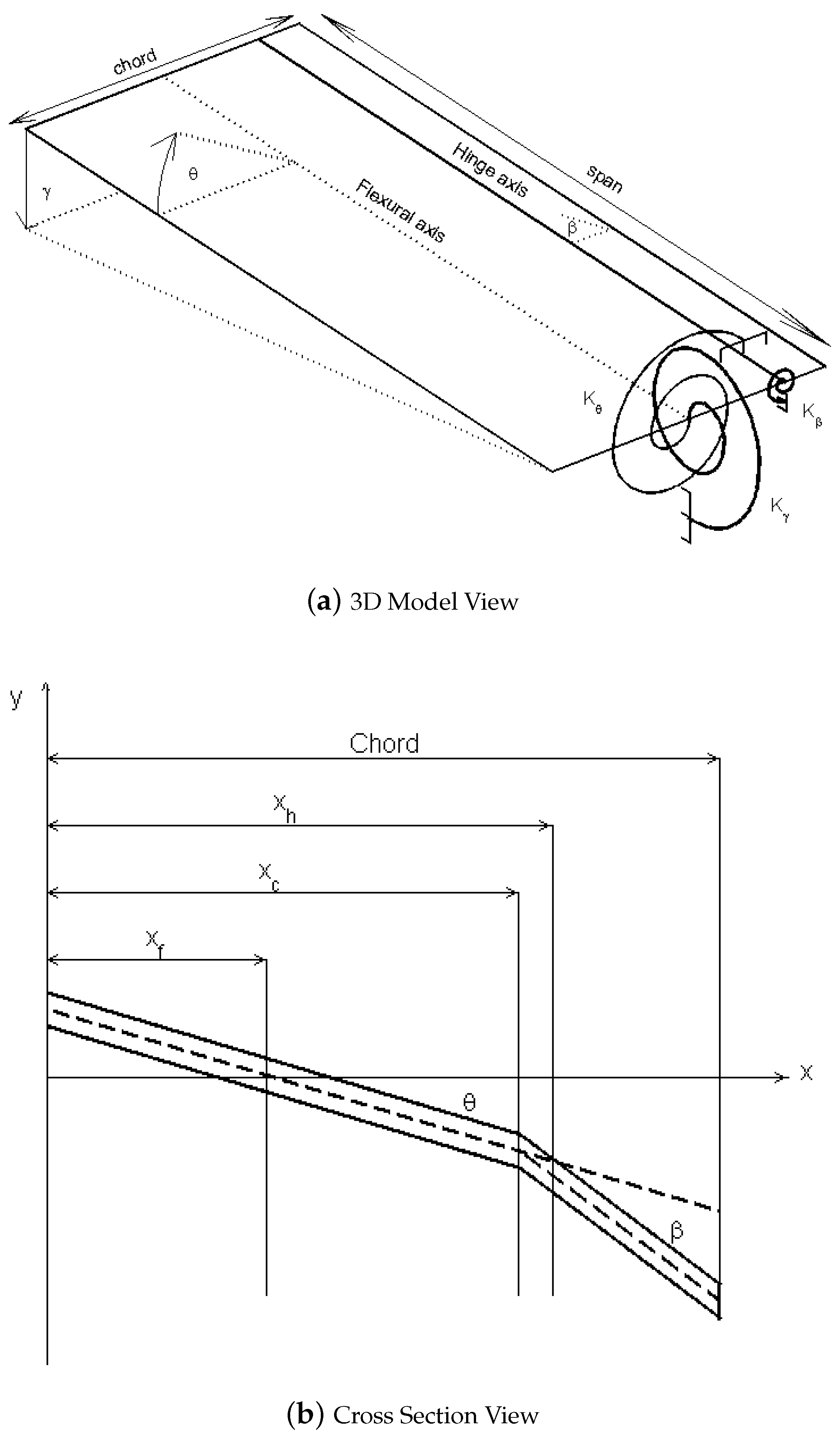
2. Theoretical Analysis

A simplified aeroelastic model is used for this study to understand the effect of transient heating on the stability characteristics of a wing in a hypersonic flow. A simple rectangular wing model [33] is defined with a pitch angle θ , flap angle γ and full-span length control surface rotation β as degrees of freedom. These degrees of freedom are introduced via three springs at the root, two along the flexural and one on the control surface hinge axis, as can be seen from Figure 1a, with the wing cross section displayed in Figure 1b.
The general equations of motion for an aeroelastic system can be written as:
A q ¨ ̲ + ( B + ρ V C ) q ˙ ̲ + ( D + ρ V 2 E ) q ̲ = Q ̲
where q represents the displacement vector, q ˙ ̲ represents the velocity vector and q ¨ ̲ represents the acceleration vector of the system, A is the inertia matrix, B and D are the structural damping and stiffness matrices, C and E are the aerodynamic damping and stiffness matrices, respectively, ρ is the air density, V is the aircraft velocity and Q is the external force excitation vector. Using the axis system defined in Figure 1b, the vertical displacement of the wing, z w , can be written as a function of the x and y positions as well as the angles, γ , θ and β . Assuming all displacement angles are small, we get the following expression:
z w ( x , y ) = y γ + ( x x f ) θ
Furthermore, the vertical displacement for the control surface can be defined as:
z c ( x , y ) = y γ + ( x x f ) θ + ( x x h ) β
With the geometric equations defined, the equations of motion can be developed using Lagrange’s equation, which for multi-degrees-of-freedom can be defined as
d d t T e q ˙ + U q = Q x = ( δ W ) ( δ q )
where Q x is the external forces on the system, W is the work done on the system, T e is the kinetic energy of the system and U is the potential energy of the system. The resultant equations of motion are
I γ I γ θ I γ β I γ θ I θ I θ β I γ β I θ β I β γ ¨ θ ¨ β ¨ + K γ 0 0 0 K θ 0 0 0 K β γ θ β = Q γ Q θ Q β
Note that I i is the inertia in the respective i-th degrees of freedom, including coupling moments, K γ , K θ and K β represent the stiffness of the restraining spring in each degree of freedom. Since the wing is completely rigid, the structural flexibility is implemented through the stiffness coefficients. The flutter speed can be easily obtained by solving the eigenvalue problem of Equation (1). In a nonlinear context, in this article, flutter will refer to an unstable oscillation.

2.1. Aerodynamic Model

In the high Mach number flight regime, the pressure distribution across the wing is significantly influenced by the presence of a shock wave. Piston theory (PT) is a modelling technique, which depends on the premise that the pressure on a wing surface can be assumed to be equivalent to the movement of a piston in a column of air. For a 2D wing section, this gives:
p ( x ) = p 1 + γ 1 2 w ( x ) a 2 γ , γ 1
where w ( x ) is the downwash seen along the wing, a is the free-stream speed of sound and γ is the gas constant. Equation (6) provides an exact solution for an expansion and an approximate solution for a compression due to the presence of the shock wave. However, the power term 2 γ γ 1 provides computational difficulty, therefore, as outlined by Lighthill (1953) [34], an approximate solution can be obtained accurate to within 0.06% of the given value using the third order binomial expansion:
p ( x ) = 1 + γ w ( x ) a λ + γ ( γ + 1 ) 4 w ( x ) a 2 λ 2 + γ ( γ + 1 ) 12 w ( x ) a 3 λ 3
λ in Equation (7) is defined as
λ = M M 2 1
where M is the free-stream Mach number and is related to the free-stream velocity V via the relationship M = V / a . In this article, all computations are performed at sea level, where a 340 ms 1 . One should note that, based on Equation (1), the solution is “non-matched”, thus disconnecting the aerodynamics calculated, i.e., matrices C and E, form the fight condition, i.e., ρ and V . The pressure can be integrated across the chord and strip theory can be used to generalise the solution for the 3D wing [35]. Now that the pressure distribution is known along the wing surface, the lift and moment coefficients can be evaluated.

Aerodynamic Coefficients

The lift ( L ) across a 2D aerofoil section is defined as the summation of the difference in pressure, Δ p , of the upper and lower surface along the chord:
d L = 0 x c Δ p d x + x c c Δ p d x
Equation (9) includes the lift contribution from the wing and control surface. Similarly, the expression for the moment about the flexural axis ( M f a ) and the hinge moment ( M h a ) due to the control surface can be defined by:
d M f a = 0 x c Δ p x x f d x + x c c Δ p x x f d x
d M h a = x c c Δ p x x h d x .
Substituting the binomial expansion for pressure into Equations (9)–(11) gives the expressions for the lift and moments across the aerofoil chord. Strip theory is then used to generalise the forces and moments across the entire wing. Strip theory is performed by integrating the lift and moment coefficients along the span:
L = 0 s d L y δ γ M f a = 0 s d M f a δ θ M h a = 0 s d M h a δ β .
The solution of the strip theory equations gives the aerodynamic model for third order piston theory. Strip theory was verified by Jones and Gallagher [35] in which they confirmed the “surface pressure distribution to be predicted using strip theory with reasonable accuracy up to angles of attack of 27 ”. Their analysis included Mach numbers up to around 6, similar to those used in this study.

2.2. Temperature Model

Aerodynamic heating of a vehicle at a given flight condition changes a number of physical parameters that affect the response of the aeroelastic system of equations [36]. Heating the structure results in a reduction in stiffness. This reduction in stiffness is due to the deterioration in the elastic modulus property of the material with increase in temperature. Furthermore, due to the expansion of a material under heat, the inertia will change with varying temperature gradients. The inertia equations can be solved using geometric discretisation [37]. This method allows the evaluation of inertia for the expansion of individual panels due to a non-uniform applied temperature distribution.
The thermodynamic model does not consider the chemical reactions, such as dissociation and ionisation, present in the free-stream at hypersonic speeds [38]. The focus of the article is on the effect of transient temperatures on the response of a wing.

2.2.1. Modelling the Structural Thermal Expansion

A beam of constant cross-sectional area under uniform heating conditions can be assumed to expand according to the following relationship:
l n e w = l ( 1 + α m Δ T )
where l n e w is the length of the beam under an increase in temperature Δ T , and l is the original beam length at a reference temperature, T r e f = 288 K. The linear thermal expansion coefficient is defined as α m . The above thermal expansion methodology can be adapted and applied to all the individual panels in the model. Therefore, the expansion of each panel becomes a function of the temperature applied to that panel only. The number of panels has to be sufficiently large enough to capture the details of the applied temperature distribution.

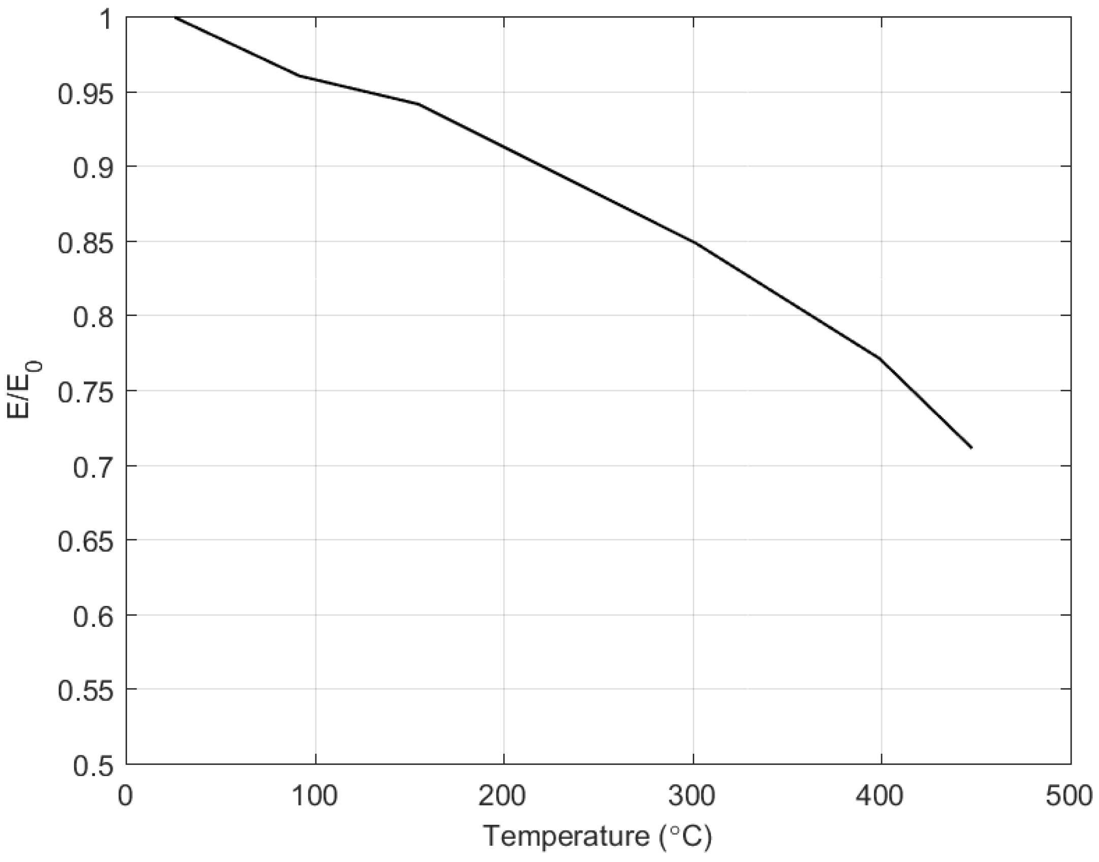
2.2.2. Modelling of Heat Effects on Stiffness

Vosteen [39] showed that it is appropriate to use the dynamic reduction in Young’s modulus with varying temperature for aeroelastic structures. The variation is shown in Figure 2. In the current work, this method is developed for determining the equivalent stiffness reduction in K γ , K θ and K β that represents the structural stiffness reduction due to the applied temperature loads. The dynamic modulus E is defined as a function of the oscillating frequency, ω :
E = 4 π 2 l 4 Γ A ω 2 λ 2 I i ( 1 + α m Δ T )
where Γ and A are material and geometric properties of the structure, namely specific weight and cross-sectional area, and I i are the moment of inertia of the respective degrees-of-freedom. The above equation can be rearranged to obtain the natural frequencies under a heat load for a particular mode:
ω n = E λ 2 I i ( 1 + α m Δ T ) 4 π 2 l 4 Γ A
where E is extracted from Figure 2, given the reference Young’s modulus E 0 . The heated natural frequency, ω n , for each mode can be used to obtain the heated values for K γ , K θ and K β using the following equation:
K i = ( 2 π ω n i ) 2 I i
where i represents the respective mode of vibration and I i is the heated moment of inertia of each mode.

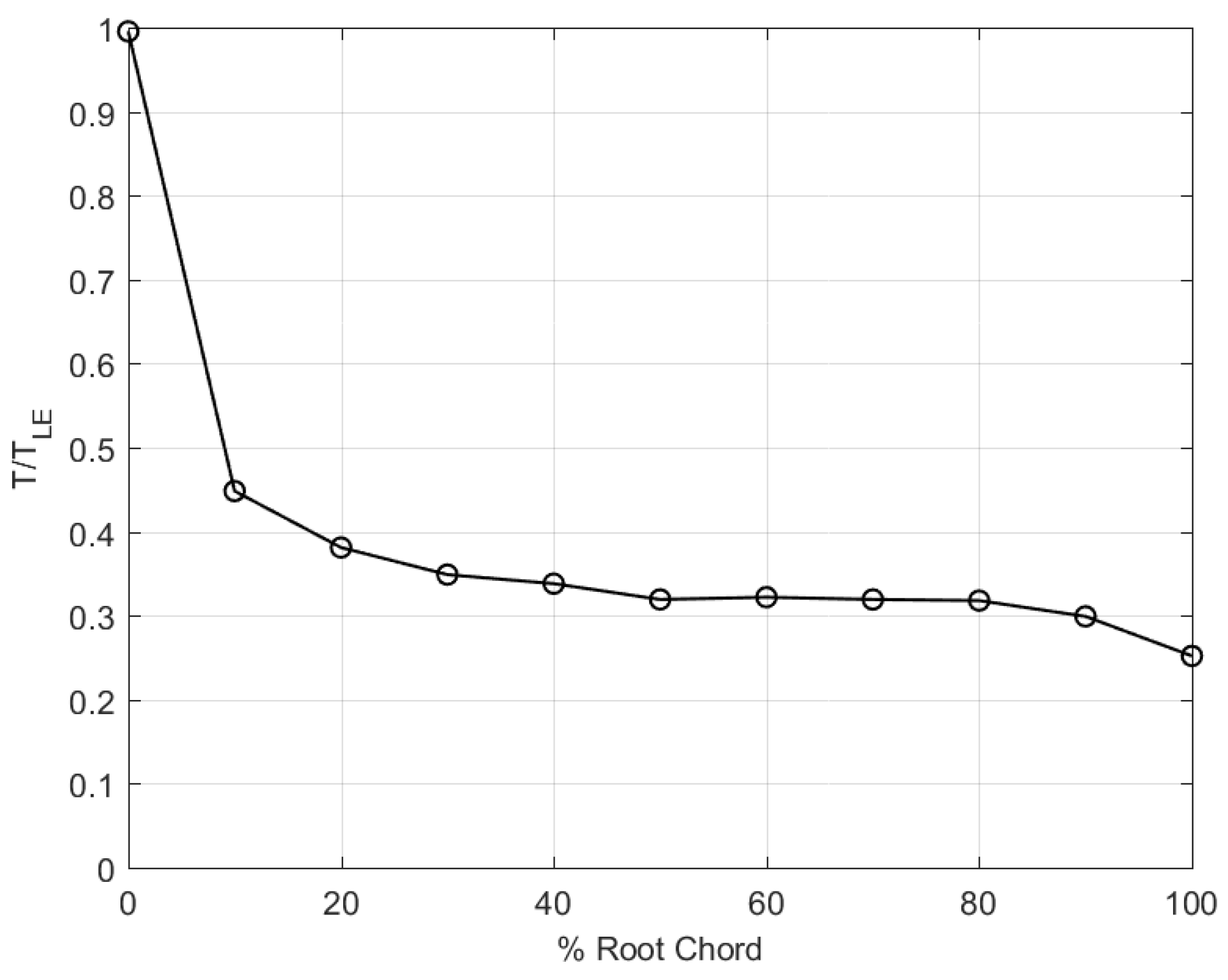
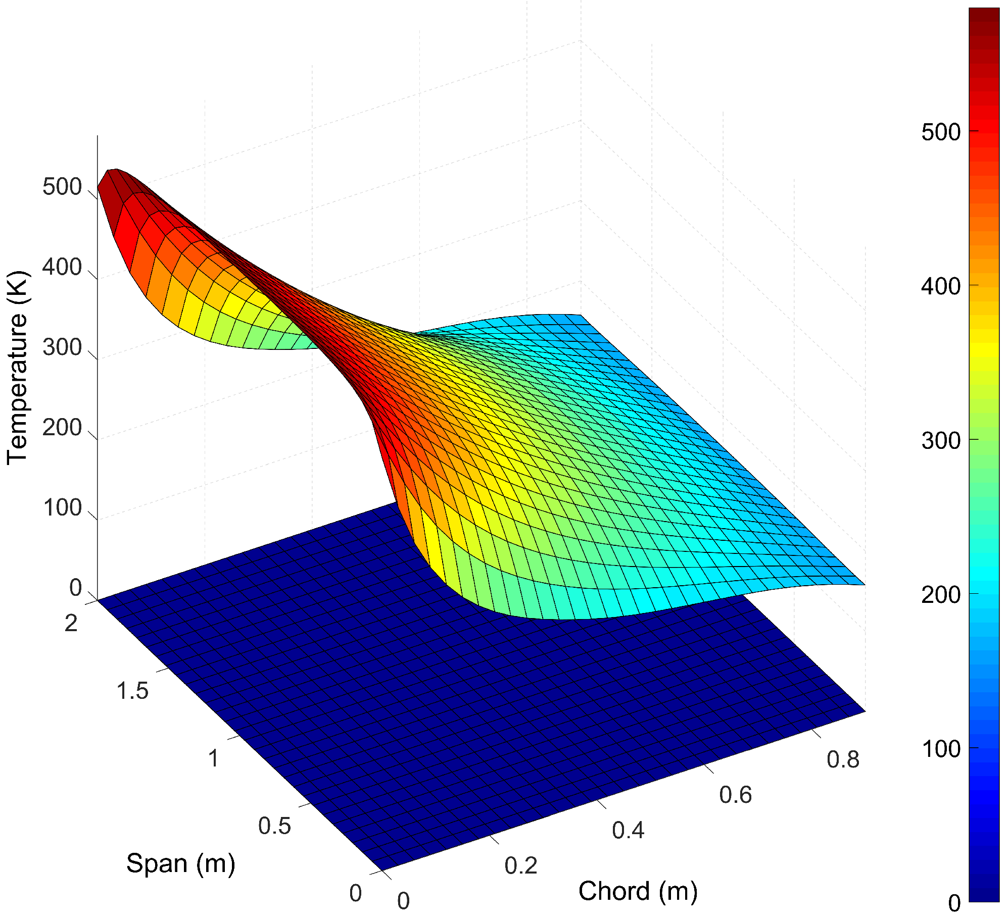
2.2.3. Temperature Distribution
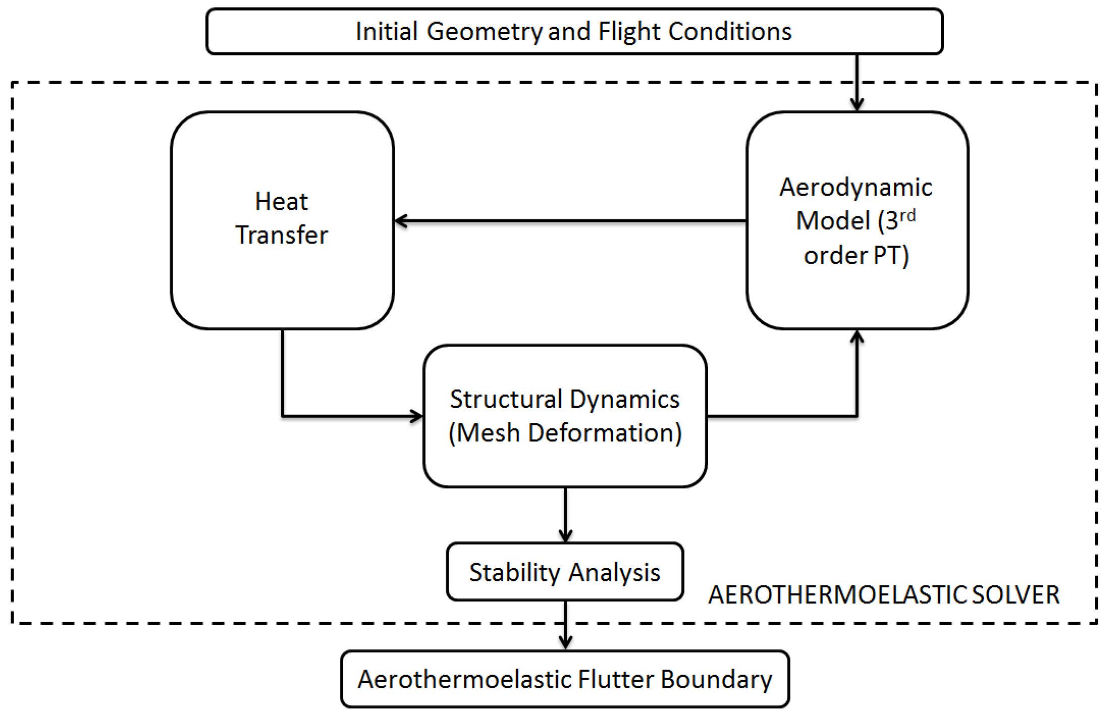
The temperature distribution was applied by approximating experimental data gained from the X-15 aircraft [40]. A temperature distribution representing a leading edge concentrated temperature is used in this study. This is to mimic a realistic temperature distribution at hypersonic speed.
The temperature distribution shown in Figure 3 can be applied to the aeroelastic model of the wing through a panel discretisation method. This allows any temperature distribution to be implemented varying over the span and chord. Since the aeroelastic model used assumes a small thickness, the temperature gradient across the thickness of the plate is considered to be orders of magnitude less than that across the chord and span. Therefore, the gradient across the thickness of the plate is assumed to be uniform for each panel.
The temperature model considers conduction through the wing and convection between the wing and the surrounding medium. This is modelled by using the unsteady heat equation in two dimensions:
T t = α 2 T x 2 + 2 T y 2 + q h ˙
This equation is a simplification of the Navier–Stokes energy equation [32], where the heat source term q h ˙ is the heat flux due to convection, which can be evaluated by:
q h ˙ = v ( T w T ) x
where v is the velocity of the air over the wing, T w is the plate temperature and T is the medium temperature. The convection coefficient can be evaluated using the Blasius solution [41], assuming the boundary layer is turbulent:
h = k V ν x ( 0.664 P r 1 / 3 )
where k is the thermal conductivity of the surrounding medium, ν is the kinematic viscosity, V is the airspeed, x is the characteristic length and P r is the Prandtl number. The model assumes a constant airspeed; however, it updates the temperature of the surrounding medium to uphold the energy balance ( q i n = q o u t ). Figure 4 shows the evolution of the temperature distribution after 1 s based on the initial conditions defined by the temperature distribution curve in Figure 3. Note that the distribution is for the entire span to have symmetry on the wing’s root plane. As expected, the leading edge is hottest due to stagnation conditions ( 500 K), with the temperature dropping by over 300 at the trailing edge. If one looks at Figure 2, there is a 70% difference between leading and trailing edge temperature. Figure 4 shows that thermal equilibrium is being achieved, as the temperature difference between leading and trailing edge after 1 s is 40 % .

2.3. Model Coupling

Although the time scale between heat, aerodynamics and structure are of an order of magnitude apart, tight coupling is required to achieve a converged and accurate solution. To achieve this, the coupling scheme illustrated in Figure 5 was constructed. The thermodynamic, aerodynamic and structural dynamic models are coupled together at every time step, such that the structural deflection updates the aerodynamic loads and the resulting deformation updates the heat transfer calculations. No sub-iterations are required thanks to the simplicity of the model, hence all solutions are solved at the same time step and updated accordingly. The aerodynamics is calculated based on initial conditions, which allows for an updated thermodynamic model to be evaluated; this in turn provides an update to the structural model. Information on the deformation are used to update the aerodynamics, with the solution evolving in time, based on the heat load profile.
A similar coupling was implemented [42] to obtain an accurate structural layout for a hypersonic vehicle under steady-state loads. This is an extension of the current state of the art where a loose coupling exists [13,14].

3. Results and Discussion

Heating has a negative impact on the dynamic response of a wing. Current research has been directed to the study of steady-state temperature distribution with loose transient coupling [13,14]. Transient effects, due to the complexity of the problem, have generally been ignored. This section characterises the effect that a transient temperature distribution has on a three-dimensional wing and compares it to the steady-state case. It should be noted that, unless stated, all cold and hot simulations are nonlinear, as all the higher order aerodynamic terms are included.

3.1. Wing at Room Temperature

A wing at room temperature is analysed as a benchmark case. The linear flutter speed analysis gives a velocity of 2157 ms 1 ( M 6.34 ) [43]. This is shown in Figure 6 as the cold data points, which of course are independent of time. The effect of heat can be seen in Figure 6 as the hot data points. The hot data points show how the instantaneous flutter speed changes as the heat is applied to the simple wing model when only linear aerodynamics is considered. Application of heat has the effect of drastically reducing stiffness and hence flutter speed. The extra stability gained by the increase in the lifting area due to thermal expansion is negligible compared to the loss in stiffness. Once the wing reaches thermal equilibrium, the stability boundary remains constant.
As the system is nonlinear due to the aerodynamics, flutter does not appear until the flow exceeds an airspeed of 2240 ms 1 ( M 6.58 ) , with limit cycle oscillations appearing at an airspeed of 2170 ms 1 ( M 6.38 ) . Figure 7 shows the bifurcation plot for the cold wing.
For the cold case, the wing begins to experience limit cycle oscillations at a velocity of 2170 ms 1 ( M 6.38 ) and continues to oscillate between two bounds with increasing magnitude until an airspeed of 2240 ms 1 ( M 6.58 ) is reached at which point flutter occurs. The response, seen in Figure 7, is a simple period-1 limit cycle meaning there are no high frequencies being excited. Figure 8 shows the dynamic response of the wing at a flight speed of 2180 ms 1 ( M 6.41 ) , comparing a cold and a hot wing response at the same airspeed. It is clear that the wing does not flutter at the speed as determined from the linear analysis (Figure 6). The nonlinear terms of the aerodynamics add a stiffening effect to the model [37], thus delaying flutter.
Figure 8a shows that the cold wing response is unstable, as the response magnitude grows exponentially, whereas the response of the hot wing is undergoing limit cycle oscilations. Similarly, Figure 8b shows the dynamic response of the wing at an airspeed of 2165 ms 1 ( M 6.36 ) .
The response of the nonlinear system lags that of the linear system (Figure 8b). This is seen by comparing the times at which the system begins to decay—for the linear system decay occurs 3 s into the simulation, whereas, for the nonlinear system, decay occurs 9 s into the simulation.

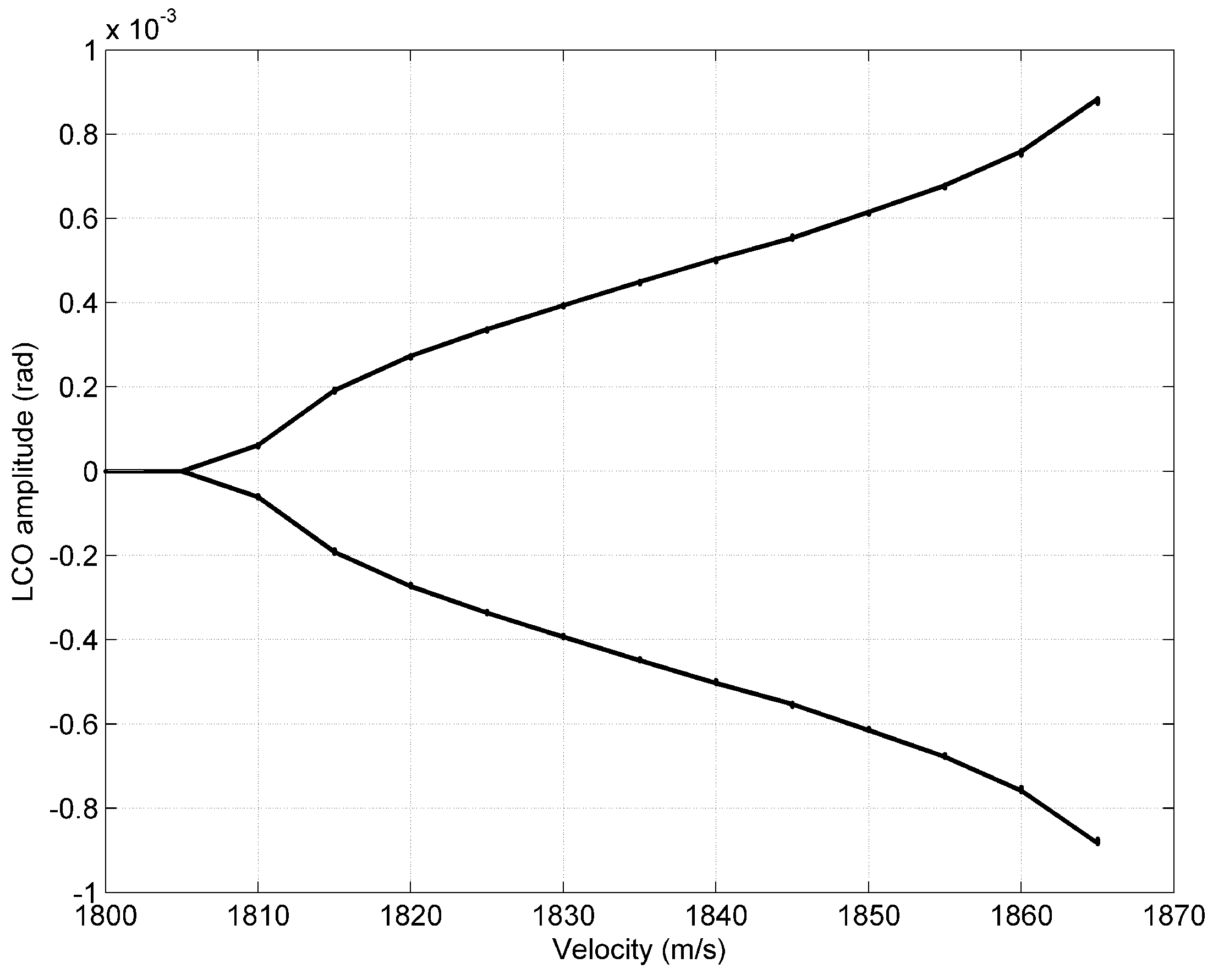
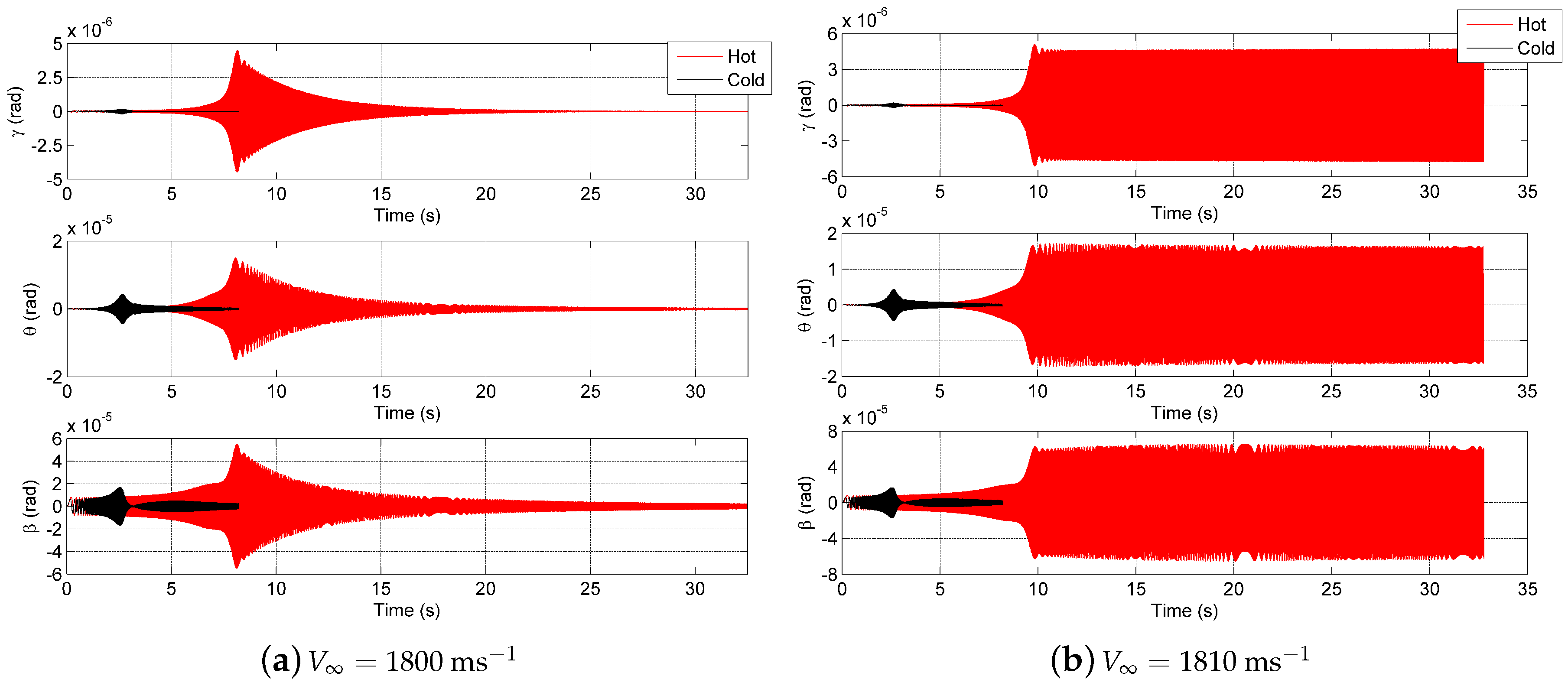
3.2. Steady-State Heat Distribution

The heat distribution shown in Figure 4 is applied to the wing model as well as the aerodynamic load. The wing temperature is initially fixed at room temperature. The linear analysis, seen in Figure 6, predicts flutter to begin at an airspeed of 1800 ms 1 ( M 5.29 ) . The results show (Figure 9) that the wing does not begin to flutter until an equivalent airspeed of 1870 ms 1 ( M 5.50 ) is reached. Limit cycle oscillations begin to occur at an airspeed of 1810 ms 1 ( M 5.32 ) . Figure 9 shows the bifurcation plot for the steady-state heat load case.
By comparing Figure 7 and Figure 9, we see that the behaviour of the two cases are similar, where the magnitude of the oscillations grow with increasing airspeed. For the hot wing case, the velocity range for which limit cycle oscillations occur is slightly smaller, 60 ms 1 compared to 75 ms 1 for the cold case. These regions are identified in the bifurcation plots by looking at the airspeed at which LCOs (Limit Cycle Oscillations) occur and unstable oscillation commence. The hot case has extra nonlinearities in the system due to changing moments of inertia, which speed up the onset of flutter. There is a significant reduction in the flutter boundary when heat is added, and the steady-state load case has a flutter speed of 1865 ms 1 ( M 5.48 ) compared to 2240 ms 1 ( M 6.58 ) for the cold case. This is attributed to the coupling of reduced stiffness and inertia effects. Similarly to the cold case, the linear analysis under-predicted the flutter speed for the steady-state heat load, 1800 ms 1 ( M 5.29 ) compared with 1865 ms 1 ( M 5.48 ) . The stiffening effect of the nonlinear aerodynamics causes this discrepancy.
Figure 10a shows the dynamic response of the wing at a flight speed of 1800 ms 1 ( M 5.29 ) . The wing passes though its first resonance under forced excitation before the wing is allowed to respond at its free behaviour, thus showing a decaying behaviour. The hot wing oscillations decay at this flight velocity, as seen in Figure 10a; however, the magnitude of the response is greater compared to the cold wing. The change in natural frequency is clearly seen from the different location of the maximum response of the wing. The cold wing has higher damping than the hot wing. At a flight speed of 1810 ms 1 ( M 5.32 ) (Figure 10b), the hot wing is now undergoing limit cycle oscillations, as the wing is oscillating between two bounded magnitudes, seen in Figure 10b, while the cold wing is presenting a decaying behaviour. Comparing the hot response to the cold wing shows that, at this velocity, under no heating, the oscillations of the wing decay and thus is dynamically stable. In all cases, the control degree-of-freedom β provides the largest response, of course all degrees-of-freedom being coupled, they all follow the same structural response, albeit at different amplitudes and frequencies. By looking at these responses, the negative impact that the heat load has on the dynamic behaviour of the wing is evident.

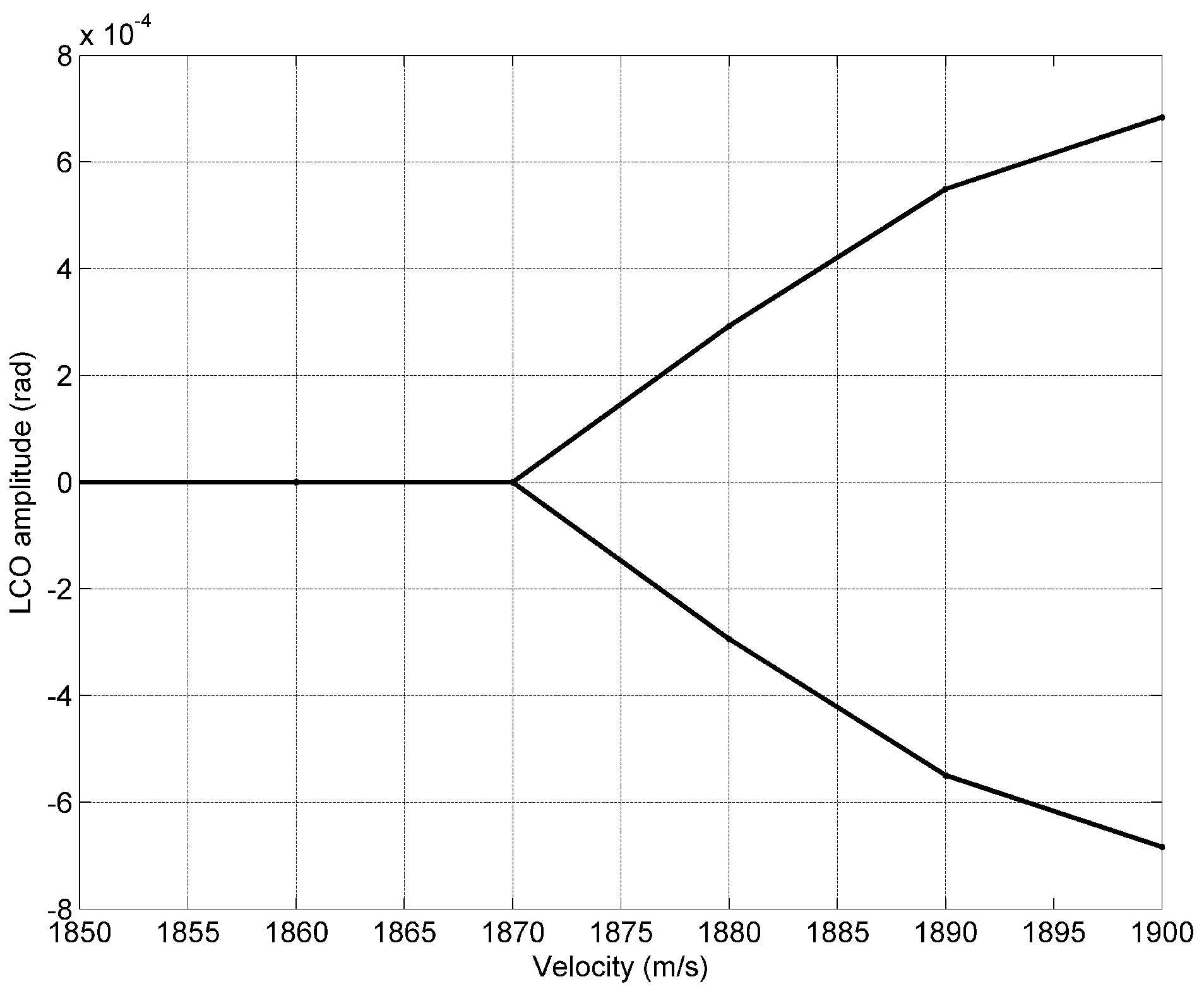
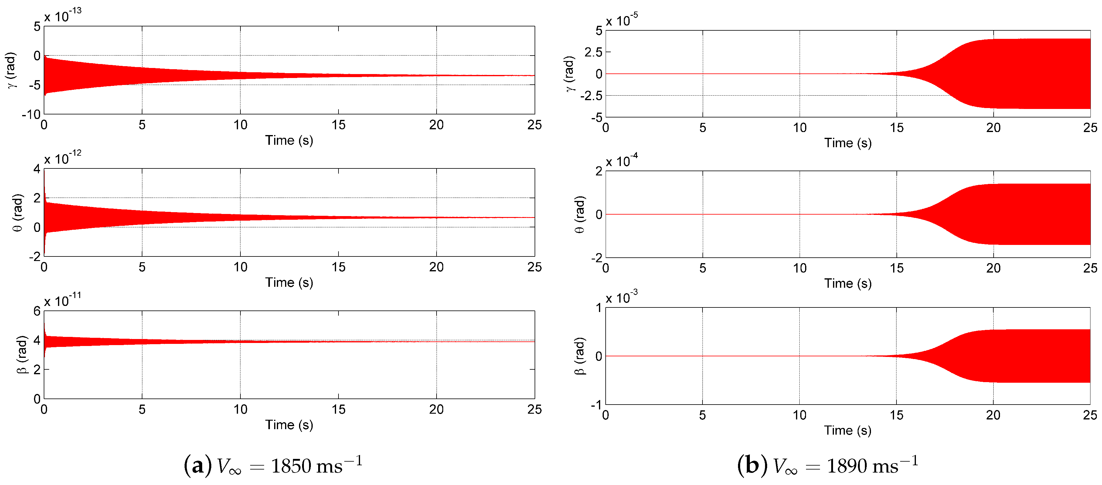
3.3. Transient Heat Distribution

The final load case applied to the wing model is a transient heat load. Since the final heat distribution is identical to the previous steady-state analysis, the linear flutter speed is the same (see Figure 6). Figure 6 shows that the airspeed at which flutter begins is reduced as heat is added to the structure, hot data points. The results of the transient solution show that the wing does not flutter until an equivalent airspeed of 1910 ms 1 ( M 5.61 ) . Limit cycle oscillations begin to occur at 1870 ms 1 ( M 5.50 ) ; this can be seen in Figure 11, which shows the bifurcation plot for the transient heat load case.
Comparing Figure 9 and Figure 11 indicates a growing magnitude of oscillation with increased airspeed. The response is still a period-1 limit cycle, therefore introducing the nonlinear heat load has not excited other high frequencies of the system. It is interesting to see that the velocity range for which limit cycle oscillations occur is further reduced for the transient heat case, 30 ms 1 compared to 60 ms 1 for steady-state. This further confirms the hypothesis of increased nonlinearity reducing the limit cycle velocity range.
Figure 12a shows the dynamic response of the wing under transient loading at a flight speed of 1850 ms 1 ( M 5.44 ) . At this flight speed under a transient temperature loading, the wing decays, seen in Figure 12a. Figure 12a emphasises how the steady-state model overestimates the hot response. Since the heat load is applied over time, as it flows through the structure, the structure dampens out the oscillations, whereas, for the steady-state model, the heat is applied instantaneously and thus reduces the damping of the wing.
Figure 12a shows the significant reduction in the magnitude of the response compared with the steady-state load case. This further emphasises the increased damping of the system. The response of the transient load case at a flight speed of 1890 ms 1 ( M 5.55 ) is given in Figure 12b. At this speed, the time varying hot wing is undergoing limit cycle oscillations, as the wing is oscillating between two bounded magnitudes. The response is significantly slower when compared with the steady-state case in limit cycle oscillations. This is seen by the time taken for limit cycle oscillations to begin, about 20 s compared to 10 s for the steady-state case.
The transient load case affects the behaviour of the response with time. Since the temperature load on the wing changes with time, the behaviour of the response changes with the heat flow. The wing initially is displaying a decaying behaviour; however, as the heat flows through the structure heating up the wing, hence changing the natural frequencies of the system, this causes the response to transition into a limit cycle oscillation. This transient behaviour is only present under a transient temperature load.

3.4. Comparison between Heat Loads

Equation (1) exemplifies that the stiffness is a function of the structure but also of the aerodynamics, which is proportional to airspeed squared. Normally, structural damping is ignored as aerodynamic damping is an order of magnitude larger, with this term being linearly proportional to airspeed. In this case, inertia is a function of heat, as the structure is allowed to expand, thus altering the inertia, and, at the same time, altering the size of the lifting surface of the model. It is interesting to note that the nonlinear aerodynamic model provides a softening effect, bringing forward the onset of the appearance of limit cycles ( V L C O ) and reducing the speed range where limit cycle occurs. The steady-state approximation provides a very conservative solution, with the results showing that the transient dynamic response of the wing is in between the room temperature and steady-state case, when comparing the flutter velocities ( V F ). The results are summarised in Table 1. The change in temperature for the transient case occurred over a longer time period, whereas the steady-state case started at a hot temperature, allowing the transient case to dampen out the oscillations. The structural response is much faster than the thermal response, milliseconds compared to seconds. This is shown in Equation (13), resulting in a larger length change and hence a greater effect occurs in the moments of inertia. Therefore, the steady-state load case overestimates the negative effects that a heat loading has on the dynamic response of a wing in predicting the instability speed.
The observed changes in the speed range for which limit cycle oscillations appear can be quantified by looking at the system restoring force. The aerodynamics provide an increase in the restoring stiffness with added nonlinearity. Figure 13 shows the restoring force plots for the two cold and hot cases considered.
The stiffness restoring force is increased with increased displacement, showing maximum values of ± 4 Nmrad. The stiffness in this displacement range displays a linear behaviour. Figure 13b shows the restoring stiffness for the hot case. It should be noted as well that damping restoring force is increased by an order of magnitude. The restoring stiffness for the hot case shows a similar behaviour to that of the cold case—this is seen by comparing Figure 13a,b, however with a larger magnitude, ± 10 Nmrad, compared with ± 4 Nmrad. This increased restoring stiffness confirms the reduction in the limit cycle oscillation velocity range for the hot cases.

4. Conclusions

A simple mathematical model has been developed to understand the effect of time and application of heat to a structure in a flowfield to represent hypersonic flight. Obviously, this model lacks many physical details, such as a boundary layer model with transition. This article is aimed at understanding the trends in stability caused by the effects of transient temperatures developed over a wing at hypersonic speed. These trends are compared with equivalent cold wing and steady-state heat loads. Further investigation will need to be performed to account for better physical modelling, especially in terms of shock wave location by using supersonic panel methods, in order to minimise computational costs. Simple transition models can be implemented to provide accurate temperature modelling.
The results show that the effects of the transient load case fall between the room temperature and steady-state solutions. The steady-state solution overestimates the effect that the heat load has on the flutter velocity. Furthermore, the transient load case shows a changing response as the heat load flows through the structure. In the 1860 ms 1 ( M 5.47 ) velocity case, the wing initially shows a decaying response followed by a transition into a limit cycle oscillation. Finally, it is observed that, as aerodynamic and thermal nonlinearities are added to the system, the system displays a higher restoring force, which results in a smaller velocity range over which limit cycle oscillations occur.
This confirms that the transient behaviour needs to be modelled when looking at the dynamic response of a hypersonic wing. The temperature effect on the flutter response cannot be ignored, and modelling the temperature load as a steady-state case will lead to over-design.

Author Contributions

D.J.M. and G.A.V. were responsible for the development of the computational model. D.V. helped in the development of the thermal model. D.J.M. performed all the computations. G.A.V. and D.J.M. are the main authors of the article with support from D.V.

Funding

This research received no external funding.

Conflicts of Interest

The authors declare no conflict of interest.

References

  1. Biot, M.A. Influences of Thermal Stresses on the Aeroelastic Stability of Supersonic Wings. J. Aeronaut. Sci. 1957, 24, 418–420. [Google Scholar] [CrossRef]
  2. McNamara, J.J.; Friedmann, P.P. Aeroelastic and Aerothermoelastic Analysis of Hypersonic Flow: Past, Present and Future. AIAA J. 2011, 49, 1089–1122. [Google Scholar] [CrossRef]
  3. Livne, E.; Weisshaar, T.A. Aeroelasticity of Nonconventional Airplane Configurations: Past and Future. J. Aircr. 2003, 40, 1047–1065. [Google Scholar] [CrossRef]
  4. Heeg, J.; Zeiler, T.A.; Pototzky, A.S.; Spain, C.V.; Engelund, W.C. Aerothermoelastic Analysis of a NASP Demonstrator Model. In Proceedings of the 34th AIAA/ASME/ASCE/AHS/ASC Structures, Structural Dynamics, and Materials Conference, La Jolla, CA, USA, 19–22 April 1993. No. 1993-1366. [Google Scholar]
  5. Heeg, J.; Gilbert, M.G.; Pototzky, A.S. Active Control of Aerothermoelastic Effects for a Conceptual Hypersonic Aircraft. J. Aircr. 1993, 30, 453–458. [Google Scholar] [CrossRef] [Green Version]
  6. Mansour, N.; Pittman, J.; Olson, L. Fundamental Aeronautics Hypersonics Projects: Overview. In Proceedings of the 39th AIAA Thermophysics Conference, Fluid Dynamics and Co-located Conferences, Miami, FL, USA, 25–28 June 2007. No. 2007-4263. [Google Scholar]
  7. Dolvin, D.J. Hypersonic International Flight Research and Experimentation (HIFiRE) Fundamental Sciences and Technology Development Strategy. In Proceedings of the 15th AIAA International Space Planes and Hypersonic Systems and Technologies Conference, Dayton, OH, USA, 28 April–1 May 2008. No. 2008-2581. [Google Scholar]
  8. Bolender, M.A.; Doman, D.B. Nonlinear Longitudinal Dynamic Model of an Airbreathing Hypersonic Vehicle. J. Spacecr. Rocket. 2007, 44, 374–387. [Google Scholar] [CrossRef]
  9. Falkiewicz, N.J.; Cesnik, C.E.S.; Crowell, A.R.; McNamara, J.J. Reduced-Order Aerothermoelastic Framework for Hypersonic Vehicle Control Simulation. AIAA J. 2011, 49, 1625–1646. [Google Scholar] [CrossRef]
  10. Crowell, A.R.; McNamara, J.J. Model Reduction of Computational Aerothermodynamics for Hypersonic Aerothermoelasticity. AIAA J. 2012, 50, 74–84. [Google Scholar] [CrossRef]
  11. Stanford, B.; Beran, P. Aerothermoelastic Topology Optimization with Flutter and Buckling Metrics. Struct. Multidiscip. Optim. 2013, 48, 149–171. [Google Scholar] [CrossRef]
  12. Lamorte, N.; Friedmann, P.P.; Glaz, B.; Culler, A.J.; Crowell, A.R.; McNamara, J.J. Uncertainty Propagation in Hypersonic Aerothermoelastic Analysis. J. Aircr. 2014, 51, 192–203. [Google Scholar] [CrossRef]
  13. Lamorte, N.; Friedmann, P.P. Hypersonic Aeroelastic and Aerothermoelastic Studies Using Computational Fluid Dynamics. AIAA J. 2014, 52, 2062–2078. [Google Scholar] [CrossRef]
  14. McNamara, J.J.; Friedmann, P.P.; Powell, K.G.; Thuruthimattam, B.J. Aeroelastic and Aerothermoelastic Behavior in Hypersonic Flow. AIAA J. 2008, 46, 2591–2610. [Google Scholar] [CrossRef]
  15. Librescu, L.; Marzocca, P.; Silva, W.A. Linear/nonlinear Supersonic Panel Flutter in a High-Temperature Field. J. Aircr. 2004, 41, 918–924. [Google Scholar] [CrossRef]
  16. McNamara, J.J.; Friedmann, P.P.; Powell, K.G. Three-Dimensional Aeroelastic and Aerothermoelastic Behavior in Hypersonic Flow. In Proceedings of the 46th AIAA/ASME/ASCE/AHS/ASC Structures, Structural Dynamics and Materials Conference, Austin, TX, USA, 18–21 April 2005. No. 2005-2175. [Google Scholar]
  17. Bisplinghoff, R.L.; Dugundji, J. Influence of Aerodynamic Heating on Aeroelastic Phenomena. Pergamon 1958, 28, 288–312. [Google Scholar]
  18. Runyan, H.L.; Jones, N.H. Effect of Aerodynamic Heating on the Flutter of a Rectangular Wing at a Mach Number of 2; Technical Report RM L58C31; National Aeronautics and Space Administration (NASA): Washington, DC, USA, 1958.
  19. Ericsson, L.; Almroth, B.; Bailie, J. Hypersonic Aerothermoelastic Characteristics of a Finned Missile. In Proceedings of the 16th Aerospace Sciences Meeting, Aerospace Sciences Meetings, Huntsville, AL, USA, 16–18 January 1978. No. 1978-0231. [Google Scholar]
  20. Spain, C.V.; Soistmann, D.L.; Linville, T.W. Integration of Thermal Effects into Finite Element Aerothermoelastic Analysis with Illustrative Results; Technical Report CR 1059; National Aeronautics and Space Administration (NASA): Washington, DC, USA, 1989.
  21. Gupta, K.K.; Ibrahim, A. Development of an Aerothermoelastic-Acoustics Simulation Capability of Flight Vehicles. In Proceedings of the 48th AIAA Aerospace Sciences Meeting, Orlando, FL, USA, 4–7 January 2010. No. 2010-0050. [Google Scholar]
  22. Gupta, K.K.; Voelker, L.S.; Bach, C.; Doyle, T.; Hahn, E. CFD-Based Aeroelastic Analysis of the X-43 Hypersonic Flight Vehicle. In Proceedings of the 39th Aerospace Sciences Meeting and Exhibit, Aerospace Sciences Meetings, Reno, NV, USA, 8–11 January 2001. No. 2001-0712. [Google Scholar]
  23. Thuruthimattam, B.J.; Friedmann, P.P.; McNamara, J.J.; Powell, K.G. Modeling Approaches to Hypersonic Aerothermoelasticity with Application to Reusable Launch Vehicles. In Proceedings of the 44th AIAA/ASME/ASCE/AHS/ASC Structures, Structural Dynamics, and Materials Conference, Norfolk, VA, USA, 7–10 April 2003. No. 2003-1967. [Google Scholar]
  24. Crowell, A.R.; McNamara, J.J.; Miller, B.A. Hypersonic Aerothermoelastic Response Prediction of Skin Panels Using Computational Fluid Dynamic Surrogates. J. Aeroelast. Struct. Dyn. 2011, 2, 3–30. [Google Scholar]
  25. McNamara, J.J.; Crowell, A.R.; Friedmann, P.P.; Glaz, B.; Gogulapati, A. Approximate Modeling of Unsteady Aerodynamics for Hypersonic Aeroelasticity. J. Aircr. 2010, 47, 1932–1945. [Google Scholar] [CrossRef]
  26. Thuruthimattam, B.J.; Friedmann, P.P.; Powell, K.G.; Bartels, R.E. Computational Aeroelastic Studies of a Generic Hypersonic Vehicle. Aeronaut. J. 2009, 113, 763–774. [Google Scholar] [CrossRef]
  27. Crowell, A.R.; Miller, B.A.; McNamara, J.J. Robust and Efficient Treatment of Temperature Feedback in Fluid-Thermal-Structural Analysis. AIAA J. 2014, 52, 2395–2413. [Google Scholar] [CrossRef]
  28. Verstraete, D.; Vio, G.A. Temperature Effects on Flutter of a Mach 5 Transport Aircraft Wing. In International Mechanical Engineering Congress and Exposition; ASME: New York, NY, USA, 2012; Volume 1, pp. 227–234. [Google Scholar]
  29. McNamara, J.J.; Thuruthimattam, B.J.; Friedmann, P.P.; Powell, K.G.; Bartels, R.E. Hypersonic Aerothermoelastic Studies for Reusable Launch Vehicles. In Proceedings of the 45th AIAA/ASME/ASCE/AHS/ASC Structures, Structural Dynamics & Materials Conference, Palm Springs, CA, USA, 19–22 April 2004. No. 2004-1590. [Google Scholar]
  30. Cazier, F.W.; Ricketts, R.H. Structural Dynamic and Aeroelastic Considerations for Hypersonic Vehicles. In Proceedings of the 32nd Structures, Structural Dynamics, and Materials Conference, Baltimore, MD, USA, 8–10 April 1991. No. 1991-1255. [Google Scholar] [CrossRef]
  31. Culler, A.J.; McNamara, J.J. Studies on the Fluid-Thermal-Structural Coupling for Aerothermoelasticity in Hypersonic Flow. AIAA J. 2010, 48, 1721–1738. [Google Scholar] [CrossRef]
  32. Cebeci, T.; Shao, J.P.; Kafyeke, F.; Laurendeau, E. Computational Fluid Dynamics for Engineers, 1st ed.; Horizons Publishing: Hammond, IN, USA, 2005. [Google Scholar]
  33. Dimitriadis, G.; Cooper, J. Limit cycle oscillation control and suppression. Aeronaut. J. 1999, 103, 257–263. [Google Scholar] [CrossRef]
  34. Lighthill, M.J. Oscillating Airfoils at High Mach Numbers. J. Aeronaut. Sci. 1953, 20, 402–406. [Google Scholar] [CrossRef]
  35. Jones, R.A.; Gallagher, J.J. Heat Transfer and Pressure Distribution of a 60° Swept Delta Wing with Dihedral at a Mach Number of 6 and Angles of Attack for 0° to 52°; Technical Report; Langley Research Centre Langley Field: Hampton, VA, USA, 1961. [Google Scholar]
  36. Varvill, R.; Bond, A. LAPCAT II A2 Vehicle Structure Design Specification; Technical Report, Long Term Advanced Propulsion Concepts and Technologies II; European Commission: Brussels, Belgium, 2008. [Google Scholar]
  37. Munk, D.J.; Vio, G.A.; Verstraete, D. Response of a Three-Degree-of-Freedom Wing with Stiffness and Aerodynamic Nonlinearities at Hypersonic Speeds. Nonlinear Dyn. 2015, 81, 1665–1688. [Google Scholar] [CrossRef]
  38. Bertin, J.J. Hypersonic Aerothermodynamics; AIAA Education Series; AIAA: Reston, VA, USA, 1994. [Google Scholar]
  39. Vosteen, L.F. Effect of Temperature on Dynamic Modulus of Elasticity of Some Structural Alloys; Technical Report; National Aeronautics and Space Administration (NASA): Washington, DC, USA, 1958.
  40. McNamara, J.J.; Friedmann, P.P. Aeroelastic and Aerothermoelastic Analysis of Hypersonic Vehicles: Current Status and Future Trends. In Proceedings of the 48th AIAA/ASME/ASCE/AHS/ASC Structures, Structural Dynamics, and Materials Conference, Structures, Structural Dynamics, and Materials and Co-Located Conferences, Honolulu, HI, USA, 23–26 April 2007. [Google Scholar]
  41. Houghton, E.L.; Carpenter, P.W. Aerodynamics for Engineering Students, 5th ed.; Butterworth-Heinemann: Oxford, UK, 2003. [Google Scholar]
  42. Munk, D.; Vio, G.; Verstraete, D. Transient Temperature Effect on the Aerothermoelastic Response of a Wing. J. Fluids Struct. 2017, 75, 45–76. [Google Scholar] [CrossRef]
  43. Stanciu, V.; Stroe, G.; Andrei, I.C. Linear Models and Calculation of Aeroelastic Flutter. UPB Sci. Bull. 2012, 74, 29–38. [Google Scholar]
Figure 1. Hancock wing model.
Aerospace 05 00071 g001
Figure 2. Variation of Aluminium 2024-T3 Young’s modulus with temperature.
Aerospace 05 00071 g002
Figure 3. Applied temperature distribution on the wing model.
Aerospace 05 00071 g003
Figure 4. Applied temperature distribution after 1 s simulation time.
Aerospace 05 00071 g004
Figure 5. Aerothermoelastic framework.
Aerospace 05 00071 g005
Figure 6. Change in flutter velocity with temperature from linear theory.
Aerospace 05 00071 g006
Figure 7. Bifurcation plot for cold wing.
Aerospace 05 00071 g007
Figure 8. Linear and nonlinear response of cold wing.
Aerospace 05 00071 g008
Figure 9. Bifurcation plot for steady-state heat load.
Aerospace 05 00071 g009
Figure 10. Wing response to steady-state heat loading.
Aerospace 05 00071 g010
Figure 11. Bifurcation plot for transient heat load.
Aerospace 05 00071 g011
Figure 12. Dynamic response of the hot system.
Aerospace 05 00071 g012
Figure 13. Restoring force plots.
Aerospace 05 00071 g013
Table 1. Summary of critical aeroelastic response.
Case V LCO (ms 1 ) V F (ms 1 )
Cold Wing21652240
Steady-State Heat Load18051865
Transient Heat Load18701900

