Abstract
Air traffic networks, where airports are the nodes that interconnect the entire system, have a time-varying and stochastic nature. An incident in the airport environment may easily propagate through the network and generate system-level effects. This paper analyses the aircraft flow through the Airport Transit View framework, focusing on the airspace/airside integrated operations. In this analysis, we use a dynamic spatial boundary associated with the Extended Terminal Manoeuvring Area concept. Aircraft operations are characterised by different temporal milestones, which arise from the combination of a Business Process Model for the aircraft flow and the Airport Collaborative Decision-Making methodology. Relationships between factors influencing aircraft processes are evaluated to create a probabilistic graphical model, using a Bayesian network approach. This model manages uncertainty and increases predictability, hence improving the system’s robustness. The methodology is validated through a case study at the Adolfo Suárez Madrid-Barajas Airport, through the collection of nearly 34,000 turnaround operations. We present several lessons learned regarding delay propagation, time saturation, uncertainty precursors and system recovery. The contribution of the paper is two-fold: it presents a novel methodological approach for tackling uncertainty when linking inbound and outbound flights and it also provides insight on the interdependencies among factors driving performance.
1. Introduction and Motivation
Air transport operations rely on a complex network architecture, where several facilities, processes and agents are interrelated and interact with each other [1]. In this large-scale and dynamic system, airports are the interconnection nodes that help aircraft distribution through the network and transport modal changes for passengers [2]. Therefore, airports represent a fundamental stage regarding efficiency, safety, passenger experience and sustainable development [3]; although they are usually a source of capacity constraints for the entire air traffic network [4]. Potential incidents, failures and delays (due to service disruptions, unexpected events or capacity constraints) may propagate throughout the different nodes of the network, making it vulnerable [5,6,7]. This situation has led to system-wide congestion problems and has worsened due to the strong growth in the number of airport operations during the last few decades [8].
The Airport Transit View (ATV) concept describes the “visit” of an aircraft to the airport [9]. This framework connects inbound and outbound flights, providing a tool to optimise airport operations and to enable more efficient and cost-effective deployment of operator resources. It integrates airside operations (landing, taxiing, turnaround and take-off) and surrounding airspace operations (holding, final approach and initial climb) [3,10,11]. Moreover, the Airport Operations Plan (AOP) guarantees a common, agreed operational strategy between local stakeholders, providing knowledge about the current situation and detecting deviations [9]. It aims to achieve early decision-making and efficient management of the aircraft processes. In this sense, the Airport Collaborative Decision-Making (A-CDM) concept ensures that common situation awareness is reached between stakeholders [9]. Moreover, the implementation of the 4D-trajectory operational concept in future Air Traffic Management (ATM) systems will impose the compliance of very accurate arrival times over designated points on aircraft, including Controlled Times of Arrival (CTAs) at airports [12,13,14].
Uncertainty of operational conditions (e.g., runway configuration, aircraft performance, air traffic regulations, airline business models, ground services, meteorological conditions) makes airspace/airside integrated operations a stochastic phenomenon [15,16,17,18,19]. It is therefore necessary to define methodological frameworks to improve predictability and reliability of the airspace/airside integrated operations. Hence, the objective of the study is two-fold: (a) to analyse and characterise the aircraft flow of processes in order to understand the uncertainty dynamics; and (b) to generate a causal probabilistic model in order to manage uncertainty in the ATV environment.
2. Background and Contribution
This paper revises two main topics: the characteristics of the airspace/airside integrated flow of an aircraft and the management of uncertainty regarding airport operations.
A previous literature review about airspace/airside integration illustrated that several prior studies have dealt with the importance of connectivity at airports [20,21,22,23,24]. The air transport network is a “time-varying network”, where the links between nodes (i.e., airports) are represented by flights on a timetable [6]. Most elements in the network are subject to stochastic influence [25,26]. The time-varying and uncertain nature of this network creates a set of “dynamics” that affect the way airlines, air navigation service providers and airports manage their operations [8,27,28]. Like other large complex networks, operations at an airport may influence other parts of the system through traffic flow [29,30,31]. Moreover, constraints at a particular airport may cause partial network degradation [6]. Hence, the flight cycle through the airport and its surrounding airspace (from inbound to outbound processes) has a significant impact on service reliability and uncertainty management within the entire air transport network. This paper revises the linkage between inbound and outbound flights by assessing aircraft operational flow (turnaround integration in the air traffic network). This approach is in line with past analyses [24,32,33,34]. Our main contribution in this field is the construction of a Business Process Model (BPM) that shapes the airspace/airside integration, by extending the spatial scope to the Extended Terminal Manoeuvring Area (E-TMA) boundaries. Instead of considering airspace and airside processes in “isolation”, our approach looks at the cross impacts between operations. In addition, the statistical characterisation of the different processes enables us to understand the particularities of the ATV. Aircraft operations are characterised by several temporal milestones, which arise from the combination of the BPM and A-CDM methodologies [35].
The stochastic nature of air traffic and airport operations at the E-TMA is mainly due to external uncertainty sources and to the intrinsic variation in the duration of processes [3,6,36]. In order to ensure continuous traffic demand at runways and maximise airport infrastructure usage, a minimum level of queuing is required. However, additional time in holdings and buffers may cause incremental delays, which are detrimental to the efficiency of operations, fuel consumption and environmental sustainability [11,16,37]. Delay dynamics and their propagation are core elements when assessing performance [28]. Apart from the associated economic costs [38], delays have a substantial impact on the schedule adherence of airports and airlines, passenger experience, customer satisfaction and system reliability [6,39]. A significant portion of delay generation occurs at airports, where aircraft connectivity acts as a key driver for delay propagation [31]. Therefore, uncertainty management and delay propagation affecting internal E-TMA and airport processes have received significant attention over previous years [4,15,24,32,40,41]. The inherent complexity of the delay propagation problem (operational uncertainty) and the intrinsic challenges in predicting an entire system’s behaviour explains the use of different modelling techniques, such as queuing theory [8,42], stochastic delay distributions [43], propagation trees [29,44,45], periodic patterns [46], chain effect analysis [47], random forest algorithms [30], statistical approaches [48], non-linear physics [49], phase changes [50] and dynamic analysis [31]. In this paper, delay propagation patterns and influence variables are characterised with a Bayesian network (BN) approach, including stochastic parameters to reflect the inherent uncertainty of the aircraft flow performance at the E-TMA. BNs are graphical probabilistic models used for reasoning under uncertainty [51,52]. This technique has proven to be an effective tool for risk assessment, resource allocation and decision analysis [53]. Moreover, BNs have unique strengths regarding cross inference and visualization [54] and have previously been used to tackle several air transport issues, such as the efficiency of air navigation service providers [55], wayfinding at airports [56], delay propagation [57,58,59], safety [60,61] and the improvement of the aviation supply chain [62]. Several studies [63,64,65] have demonstrated the utility of graph theory and BNs as methodologies for modelling the diffusion of events and incidents from the node level to the system level (interdependence of multiple factors). Moreover, Liu et al. [66], Liu and Wu [59] and Xu et al. [58] confirmed that BNs can explain how subsystem level causes propagate to provoke system level effects, specifically focusing on how delays at an origin airport propagate to create delays at a destination airport. We seek to manage uncertainty at the source through the development of a tool for better understanding of hidden dynamics in the airspace/airside integrated operations.
Consequently, the main contribution of the paper to the existing literature in the topic is the proposal of a methodological approach to (a) understand relationships between procedures at the ATV stage (development of a process model); (b) identify factors influencing performance; (c) characterise uncertainty sources; and (d) appraise the cross-dependencies among variables (development of a causal model). Following this methodological approach, a test case is discussed to obtain tangible outcomes.
3. Materials and Methods
The analysis is divided into two steps. First, we develop a theoretical appraisal of the aircraft operation within the E-TMA, by characterising the processes and structuring the different timestamps. We generate a BPM, which is combined and quantified with the A-CDM milestone approach. This provides us with a conceptual framework for the practical analysis of the ATV flow (Section 3.1). The second part of the analysis is developed with a practical case study at Adolfo Suárez Madrid-Barajas (LEMD) Airport (Section 3.2). We characterise the uncertainty sources and assess the system’s time-efficiency performance. This is achieved by statistically evaluating the processes that were previously recorded in the first step and by also appraising the behaviour of uncertainty drivers (Section 3.2.1). After that, a probabilistic causal model is assembled to consider the interactions between different uncertainty explanatory variables (Section 3.2.2). The operational relationships that shape this model arise from the previous ATV flow framework. Figure 1 shows the proposed methodological approach for uncertainty management at the ATV (airspace/airside integrated operations). It summarizes the relationships among the different analyses and models described in Section 3.
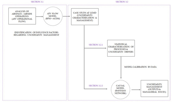
Figure 1.
Methodological approach for uncertainty management at the Airport Transit View (ATV).
3.1. Model for Airspace/Airside Integrated Operations
The evolution of a flight can be described as a sequential flow of events or processes [15,33,67]. Each of these events occurs consecutively, and if any of them are delayed, this may result in subsequent processes also being delayed (unless certain buffers or “slacks” are added into the times allocated to the completion of certain events) [6,16]. To analyse the evolution of the aircraft flow and the potential uncertainty propagation in the successive phases, this paper followed a “milestone approach” by assigning completion times to each event. This view, in line with the A-CDM method [68], allowed us to understand the operational performance and the potential saturation of the system. Saturation is here understood as the lack of capacity at the airport-airspace system level to “receive and transmit” aircraft flows according to a planned schedule. In the analysis, we used a spatial boundary associated with the E-TMA, which allowed us to consider inbound and outbound timestamps. This management boundary (airport centric limit of 200–500 NM) has already been implemented at multiple airports, with a horizon that ranges from around 190 NM for Stockholm to 250 NM for Rome and 350 NM for Heathrow [69]. The E-TMA (and not just the basic on-ground turnaround path at the airport that connects inbound and outbound flights) was selected to integrate uncertainty propagation in the airport system with global impacts in the air traffic network. This approach reflects the interaction between airport and airspace processes. The analysis focused on the aircraft flow– airside operations. Figure 2 illustrates the main processes that take place in the airport environment, using flights (up) and passengers (down) as flow agents. It describes the interaction between the airspace, airside and landside operations. Blocks highlighted in green refer to operations included in the spatial scope of the problem (aircraft flow at the airspace/airside framework). Over time, we restricted actions to tactical phases (day of operations) in order to consider the primary and initial inefficiencies of the system. The aim of the study was to describe a “visit” of an aircraft to the E-TMA (Figure 3), as an extension of the Single European Sky ATM Research (SESAR)’s ATV concept [9]. This “visit” consists basically of three separate sections [9]:
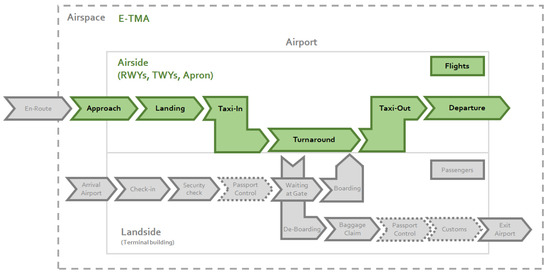
Figure 2.
Spatial scope of the problem (airspace/airside operations).
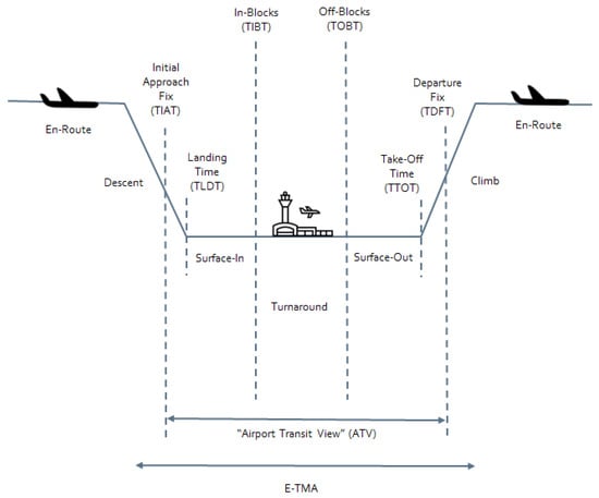
Figure 3.
Extension of the ATV concept. Adapted from [9].
- The final approach and inbound ground section of the inbound flight.
- The turnaround process section in which the inbound and the outbound flights are linked.
- The outbound ground section and the initial climb segment of the outbound flight.
The development of the conceptual structure of the aircraft flow within the E-TMA required input from various sources and consisted of four main steps [70]:
- Review of relevant literature and existing aircraft flow models [3,6,9,10,11,39].
- Hierarchical task analysis [71]. This appraisal follows a top-down approach that incorporates several sources of information to give a detailed understanding of the processes:
- (a)
- Analysis of operations manuals [72,73], standards and procedures [74,75,76,77,78].
- (b)
- Observations at Adolfo Suárez Madrid-Barajas Airport (LEMD) during 2016.
- (c)
- Structured communications with relevant stakeholders (Table 1).
 Table 1. List of informants, interviewees and contributors.
- Initial aircraft process model.
- Validation of the initial model with the help of subject matter experts (Table 1).
We employed Unified Modelling Language (UML) to graphically represent the BPM. UML is a visual modelling tool that can be used to create a pattern of a system [79]. The designed conceptual structure for the airspace/airside integrated operations is basically a UML sequence diagram (Figure 4). This framework allowed us to understand the relationships between processes in order to build the initial process model for the ATV flow and to characterise operational interdependencies in the subsequent causal model.
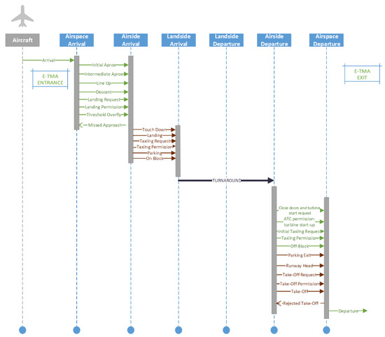
Figure 4.
Unified Modelling Language (UML) for the Business Process Model (BPM) of the aircraft flow (airport/airspace integrated operations).
This model was then compared to the operational milestones defined by the A-CDM methodology. A-CDM aims to improve the overall efficiency of airport operations by optimising the use of resources and improving the predictability of events. It focuses on aircraft turnaround and pre-departure sequencing processes [68]. The main goal of the milestones approach is to achieve common situational awareness by tracking the progress of a flight from the initial planning to the take off. It defines “timestamps” to enable close monitoring of significant events [68]. The A-CDM implementation has been proven to provide several benefits in areas such as delay/capacity management, resource allocation, operational predictability, noise abatement and fuel savings for all major stakeholders, including airlines, ground handlers and the network manager [35]. Table 2 shows the set of selected milestones along the progress of the flight using the A-CDM concept.
Table 2.
Selected milestones along the flight process (A-CDM concept). Adapted from [68].
To characterise schedule perturbations, we defined delays as “schedule delays”, the difference between a planned time and the actual time. The term “schedule delay” can refer to a difference in either the early or late direction [6]. Hence, it can be positive or negative. The milestones in Table 2 allowed us to describe delays. Each actual (A) timestamp could be checked against a scheduled (S) one, or we could assess times between two milestones (duration of the process). Therefore, five main delay measures (perturbations in operational efficiency) were considered in the characterisation of the ATV stage:
- Arrival delay: ALDT-SLDT.
- Taxi-in delay: Actual taxi-in duration (AIBT-ALDT) versus scheduled taxi-in duration (SIBT-SLDT)
- Turnaround delay: Actual turnaround time (AIBT-AOBT) versus scheduled turnaround time (SIBT-SOBT)
- Taxi-out delay: Actual taxi-out duration (AOBT-ATOT) versus scheduled taxi-out duration (SOBT-STOT)
- Departure delay: The sum of arrival upstream delay (reactionary) and the aggregated delay at the on-ground stage: system delay (primary delay), which is composed of taxi-in, turnaround and taxi-out delays. Hence, four mutually exclusive and complementary stages were evaluated to characterise the system’s schedule adherence: arrival, taxi-in, turnaround and taxi-out.
Consequently, departure delays result from various reasons, such as “inherited” arrival lateness, delayed ground processes and/or disturbed ground operations. Interdependencies exist and may affect the delay chain. Existing reactionary delay may result in an even increased follow-up delay due to scarce resources at the airport [7]. We also considered four more measures that were already included in the main delays: (a) excess approach queuing time; (b) start-up delay (ASAT-TSAT); (c) push delay (AOBT-ASAT) and (d) Air Traffic Flow and Capacity Management (ATFCM) delay. The first one of these factors was included in the arrival delay, while the other three were included in the turnaround delay. The start-up delay assessed slowness in the scheduled start-up time, while push delay illustrates the difference in time between the actual start-up approval permission by the Air Traffic Controller (ATC) and the off-block operation. ATFCM delay is due to flow and capacity regulations in which aircraft are held on ground, preventing them from encountering airborne delays during which fuel is burnt and emissions are produced [80].
By combining the BPM and the milestone approach, Figure 5 shows a conceptual diagram for the E-TMA operational environment (airport-airspace stage). This diagram allows us to
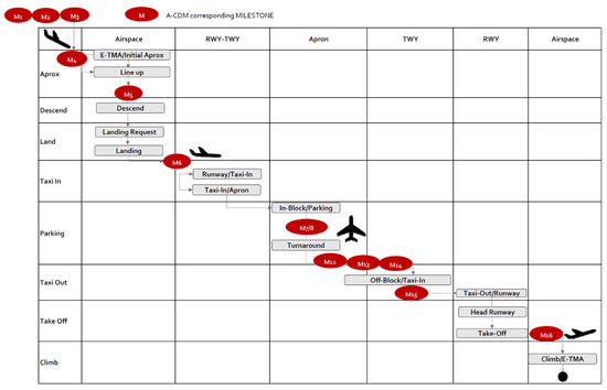
Figure 5.
Combination of the BMP for the airport–airspace integrated operations and the A-CDM concept.
- Determine significant events to track the progress of a flight (arrival, landing, taxi-in, turnaround, taxi-out and departure) and the distribution of these key events as milestones.
- Ensure linkage between arriving and departing flights.
- Assess time efficiency performance, which is measured for each milestone or between two milestones.
- Enable early decision-making when there are disruptions to an event.
- Appraise the operational relationships and interdependences between processes that will shape the structure of the causal model for uncertainty management (identify variables).
3.2. Case Study for Uncertainty Characterisation and Management at the ATV
3.2.1. Statistical Characterisation of Processes and Uncertainty Drivers at the ATV
Uncertainty sources at the ATV stage were appraised with a case study at Adolfo Suárez Madrid-Barajas Airport (LEMD) which has been integrated in the A-CDM program since 2014. The methodology could be nevertheless applied to other airports by adjusting the model to the infrastructure characteristics, the operational pattern and the available data. Figure 6 shows the layout of LEMD, with four runways (36L-18R, 36R-18L, 32L-14R, 32R-14L), four terminal areas (T123, T4T4S, general aviation and cargo) and 163 aircraft parking stands [81]. The operational preferential configuration at LEMD is the north configuration, with arrivals from runways 32L/32R and departures from runways 36L/36R. The non-preferential configuration (south) has arrivals from runways 18L/18R and departures from runways 14L/14R. Night flights (between 11 p.m. and 7 a.m. local time) use 32R (arrivals) and 36L (departures) for the north configuration and 18L (arrivals) and 14L (departures) for the south configuration [81]. LEMD can be considered a major connecting hub, where several airlines have a significant presence at the airport with a business model for transferring passengers between arriving and departing flights [82].
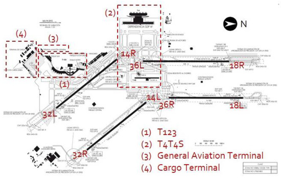
Figure 6.
Functional structure of Madrid airport (LEMD). Adapted from [81].
The observation period corresponds to July and August 2016, when 67,678 aircraft movements (arrivals and departures) were registered at LEMD. Therefore, a collection of nearly 34,000 turnaround operations was used to describe the aircraft flow characteristics, through a statistical analysis of the processes. The size of the sample allowed us not only to perform a representative post operational analysis but also to develop reliable predictions regarding schedule adherence and to study the interdependencies between the turnaround processes and the different involved variables.
The data preparation phase covered all activities required to arrange the final dataset from the initial raw meteorological, radar and airport operational data, including locating and refining erroneous measurements. As shown in Table 3, the final dataset included information about airport infrastructure allocated to each operation, airline and aircraft characteristics, flight details, route origin and destination, operational times (milestones and duration of processes), regulations, causes of delay and meteorological features. Data regarding the aircraft and the flight (type, call sign and registration number) enabled us to link the inbound and outbound movements, assessing their “turnaround” operation (i.e., trace the airport–airspace integrated operations).
Table 3.
Information included in the final dataset (obtained from raw data or derived from it).
Each of the elements included in the final dataset (Table 3) was statistically appraised and fitted to a probability density function. Six different statistical distributions were found to be candidates: Weibull, Gamma, Beta, Gumbel, F and Normal. The K-S test and χ2 goodness-of-fit test were used to ensure the “power” of curve fitting [83]. Fricke and Schultz [32] and Wu [6] previously found this procedure to be efficient when analysing on-ground processes. When a parametric distribution could not properly describe the data, we used a Kernel density estimation approach to obtain a nonparametric representation of the probability density function of the variable [84]. See Figure 7 and Figure 8 for some examples.
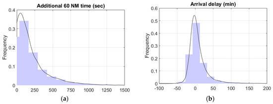
Figure 7.
Histogram and distribution fitting for (a) additional time at ASMA 60 NM (s); (b) arrival delay (min).
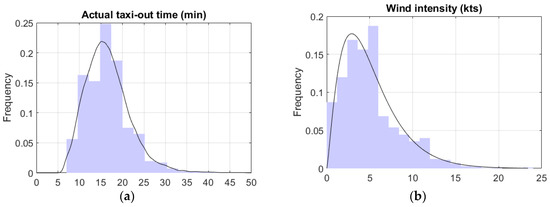
Figure 8.
Histogram and distribution fitting for (a) actual taxi-out time (min) and (b) wind intensity (kts).
Distribution fitting has four main objectives: (a) to characterise the operational environment (e.g., duration and starting time for each process); (b) to appraise delays, uncertainties and their statistical behaviour; (c) to use probability distributions as a tool for dealing with uncertainty in order to make informed decisions and predictions (e.g., cumulative density functions can be used for allocating turnaround and buffer times); and (d) to model uncertainty sources when feeding the causal model that is developed later. As an example, Figure 9 shows the analysis for the turnaround stage (actual process length and in-block/off-block adherence) as it was found to be essential when assessing the system’s ability to absorb delays [16]. Although the sample was rather heterogeneous (a range of 746 min, due to aircraft parked overnight), almost 67% of its turnaround operations last less than 120 min. Thirty-four percent of operations fall within the interval from 30 to 60 min. The mean, median and mode for the turnaround’s length are 166 min, 78 min and 54 min, respectively. For the purpose of our paper, aircraft turnaround activities were treated aggregately as a “single” process or “black box”. This approach provided us with a “macro” view of aircraft turnaround operations and simplified the observation and modelling work needed to study interdependencies in the subsequent causal analysis [6].
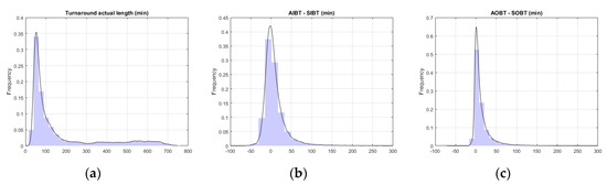
Figure 9.
Histogram and distribution fitting for turnaround: (a) actual duration (min); (b) starting time delay (AIBT–SIBT) (min); and (c) finishing time delay (AOBT–SOBT) (min).
Figure 10 illustrates the “pure” turnaround delay (without considering ATFCM regulations) characteristics. A delay at the “pure” turnaround stage could adequately be represented with a normal distribution (μ = 0.9 min, σ = 30.3 min), and is expressed with the following probability density function:
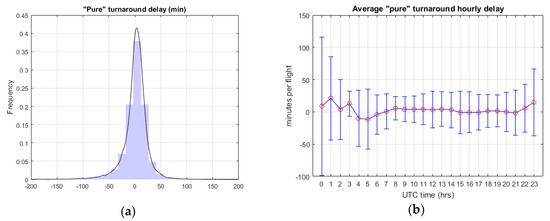
Figure 10.
“Pure” turnaround delay (without considering the ATFCM delay): (a) histogram/curve fitting and (b) average hourly delay (min/operation) throughout the day (the error bars denote intervals of one standard deviation).
Fitting turnaround characteristic times to a statistical distribution may help in the definition of an operational buffer or “slack” (balancing trade-offs between schedule punctuality and aircraft utilisation) with the final objective of absorbing arrival delay. When designing the optimal turnaround time, curve fitting should be adjusted to different clusters (types of fleets, airline operators, routes), as each of them presents different patterns.
Figure 11 represents a plot of the quantiles of the sample data (“pure” turnaround delay) versus the theoretical quantiles values from a standard normal distribution. The plot appears linear between −2 and 2 times the standard deviation (95% of the distribution). Therefore, the metric related to “pure” turnaround delay was described with a normal distribution for reasonable operational times (−20 min to 100 min). The rest of the data can be understood as outliers (unusual operations) that distort the distribution.
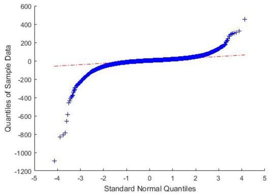
Figure 11.
Quantile-quantile plot of sample data (“pure” turnaround delay) versus standard normal.
3.2.2. Causal Model for Uncertainty Management at the ATV
The study was completed with a causal analysis through a Bayesian network (BN) approach, which aimed to understand the interdependencies between factors influencing schedule adherence and uncertainty management (drivers and predictors).
A BN is a directed acyclic graph (DAG) in which each node denotes a random variable and each arc denotes a direct dependence between variables (nodes that are not connected symbolize variables that are conditionally independently of each other) [85]. The DAG that results from the construction of a BN is quantified through a series of conditional probabilities based on the data or information available on the system or problem. It defines the factorization of a joint probability distribution by the variables represented in the DAG [54,86,87]. The factorization is represented by the directed links in the DAG [88]. That is, each node is associated with a probability function that takes (as input) a particular set of values for the node’s parent variables, and gives (as output) the probability (or probability distribution, if applicable) of the variable represented by the node [87]. Therefore, the BN model structure (nodes and arcs) encodes conditional dependence relationships between the random variables. Each random variable is associated with a set of local probability distributions (parameters in the Conditional Probability Tables, CPT). The probability information in a BN is specified via these local distributions [54]. Consequently, a BN is a pair (G, P), where G is the DAG defined by a set of nodes x (the random variables), and P = {p(x1│π1), … p(xn│πn)} is a set of n conditional probability densities (CPD), one for each variable. πi is the set of parents of node xi in G. Set P defines the associated joint probability density of all nodes with the following equation (the chain rule for BNs) [52,85]:
Graph G contains all of the qualitative information about the relationships between the variables, regardless of the probability values assigned to them. Additionally, the probabilities in P contain quantitative information, i.e., they complement the qualitative properties revealed by the graphical structure [54,86,87]. Figure 12 gives a basic example of a BN, where X2 and X3 are parent nodes of X4 (child node for X2 and X3). The probability distribution of X4 depends exclusively on the value of its parent variables (X2 and X3), i.e., X4 is conditionally independent of X1 given knowledge of X2 and X3.
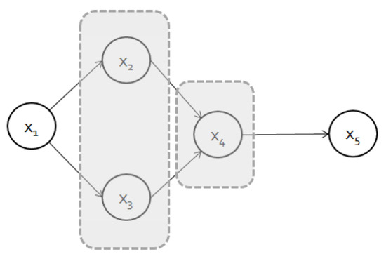
Figure 12.
Example of causal inference in a Bayesian network (BN).
A BN can be constructed either manually, based on knowledge and experience acquired from previous studies and literature, or automatically from data [85]. In this study, the selection of variables (Table 4) was constrained by the availability of data. We used the elements (timestamps, meteorological features, aircraft and airline data, flight details, operational characteristics and airport configuration) that were analysed and modelled throughout the study. The proposed construction process for the BN is depicted in Figure 13.
Table 4.
List of variables represented in the causal model (nodes at the BN).
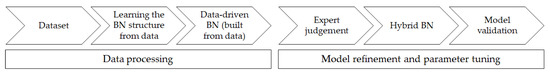
Figure 13.
BN construction process.
The first step in the BN construction process was to generate a correlation matrix for the variables involved in order to assess the correlation among pairs (regression analysis). Nevertheless, correlation does not imply causation [89]. Although, in a BN model, it is not strictly necessary to include directed links in the model following a causal interpretation, it does make the model much more intuitive, eases the process of getting the dependence and independence relations right, and significantly facilities the process of eliciting the conditional probabilities of the model [85]. Therefore, proper modelling of causal relationships (i.e., the directed links represent causal relations) is helpful for the model construction. For our purpose, causality was understood as follows: a variable X was said to be a direct cause of Y if the value of X was set by force. The value of Y may change and there is no other variable Z that is a direct cause of Y, such that X is a direct cause of Z (see Pearl’s work for details) [89]. The discretization of variables was based on the statistical characterization previously developed. It is a crucial step to improve the model’s accuracy, especially with “time” nodes (e.g., when a node represents a delay in the process, discretization must ensure that we neither lose information, nor consider an excess of states). In some “target” nodes (e.g., departure delay), the discretization was made not only according to data distribution but also to potential operational objectives (e.g., the ±3 min threshold for departure punctuality set by SESAR’s performance metrics [90]).
Subsequently, a data-driven process was used to build the BN, applying a Bayesian search (BS) algorithm [85,91]. This algorithm essentially follows a hill climbing procedure (guided by a scoring heuristic) with random restarts. It has been proven to be highly effective in inter-causal propagation problems like the one we were facing [92,93]. The BS algorithm uses the BDeu (Bayesian–Dirichlet equivalent uniform) function as the network scoring function in its search for the optimal graph. It measures how well its structure probabilistically represents the data used to build it. This scoring function is a common tool for selecting between different statistical models and it represents the goodness of fit of the model to observed data [94]. Apart from this scoring metric, network candidates were also judged based on several criteria, including network structure simplicity (with simpler networks preferred) and the ease by which the network could be implemented in simulations of ATV operations. Basically, we reach a trade-off between simplicity (minimum number of nodes required to perform accurate predictions) and the inclusion of all the significant nodes (to be able to appraise their influence).
The final step consisted of validating the network structure with the judgment of key experts in the field (detailed in Table 1). The final architecture presented in Figure 14 was hence determined by applying the BS algorithm (including variable discretization and validation) and then refining it with previous knowledge (inputs from the subject experts). The nodes in Figure 14 refer to Error! Reference source not found. Therefore, our model was built through a combination of a data-driven process and practical adjustments, in order to obtain a model reflecting reality. We developed a statistical significance test on pairs of nodes connected by an arc in the BN. Associations between the nodes were statistically significant at p = 0.02.
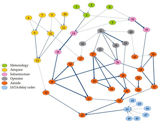
Figure 14.
BN model to understand the interdependencies between factors that influence delay performance and system saturation. Colours represent different BN layers.
The BN structure is represented in Figure 14 using the tool GeNIe [91]. The thickness of an arc represents the strength of influence between two directly connected nodes. We used two measures of distance between distributions to validate results: Euclidean and Hellinger [95].
The BN was organised in different layers attending to the nature of the data (see Table 3 and colours in Figure 14 identifying set of factors). This classification allowed us to understand the causal relationships among influence parameters. The aim was to organise the analysis of the impact for each category when assessing causality and managing uncertainty.
- Nodes 1–5 represent meteorological conditions.
- Nodes 6–13 include data regarding the arrival airspace: timestamps and congestion metrics (throughput, queues and holdings).
- Nodes 14–15, 26 and 38–39 illustrate infrastructure information.
- Nodes 16, 22–25 and 40 refer to operator, aircraft, route and flight data.
- Nodes 17–21, 27–37 and 41–42 include data regarding airside operational times and regulations.
- Nodes 43–49 represent delay causes according to the IATA coding system [74].
Due to the conditional dependence relationships of the variables within the network, BNs offer the ability to either predict or diagnose (i.e., they can determine effects and causes). Therefore, two main scenarios reflect the utility of the model in uncertainty management:
- Scenario 1 (forward/inter-causal scenario). The model predicts departure delay (output-child node) by setting the probability of having a certain configuration, i.e., by setting one or more parent-input nodes.
- Scenario 2 (backward inference). The model delivers a particular configuration in the parent nodes by setting the delay node to a target value. It provides understanding about the main contributors to delay (if delay is settled to a high positive value) or what configuration optimises operations (if delay is settled to a negative value).
Hence, the causal model (BN) can be used as a decision-making tool for resource allocation and for optimisation of operational strategies regarding delay management. Nevertheless, it is not always possible to act on all the parameters (e.g., runway configuration is set by wind direction) or combine all the variables (e.g., terminal areas are assigned to specific airline alliances).
We performed a k-fold cross-validation procedure for the BN results [96]. The original sample was partitioned into k equal sized subsamples. Of the k subsamples, a single subsample was retained as the validation data for testing the model, and the remaining k − 1 subsamples were used as training data. The training and test subsamples were randomly selected from the complete dataset. We set k = 10; hence, a sub-sample of 90% of the observations was selected to train/build the model structure (i.e., establish the model’s ability to explain delay propagation). The remaining 10% of the data was set aside to test the accuracy of the predictions made by the model (i.e., to test the model’s predictive capacity). The cross-validation process was then repeated k times (the folds) with each of the k subsamples used exactly once as the validation data.
Figure 15 shows the receiver operating characteristic curves (ROCs) which illustrate the model’s diagnostic ability by plotting the true positive rate against the false positive rate at various threshold settings [91,96,97]. The best possible prediction method will yield a point in the upper left corner [coordinate (0,1)] of the ROC space, representing 100% sensitivity (no false negatives) and 100% specificity (no false positives). Points above the diagonal line represent good classification results (better than random).
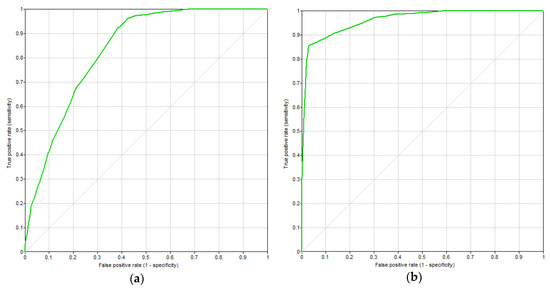
Figure 15.
Receiver operating characteristic curves (ROC) curves for predicting (a) departure delays between 3 and 15 min and (b) departure delays over 15 min.
The appraised scenarios provide promising results regarding the model’s ability to manage uncertainty (by explaining the system’s performance and predicting delay propagation). The test error ranged between 6% and 17%, with an average value of 10%. The highest test error appeared in cases with extreme values for delays and uncertainty sources. This suggests that over-sampling (i.e., deliberate selection of individuals of a rare type for the training set), instead of random sampling, could be a good methodological improvement in future works.
4. Results and Discussion
This section illustrates the outcomes that have arisen from previous models: (1) the operational framework for the ATV stage (including the statistical characterisation of processes and uncertainty drivers); and (2) the causal model for uncertainty management (BN). These tools allowed us to understand the hidden dynamics of the airspace/airside integrated operations for the case study. Figure 16 depicts the linkage between the methodological approach (Section 3) and the results of the analysis (Section 4).
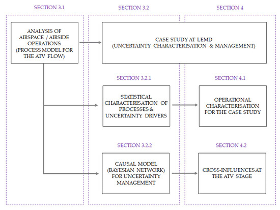
Figure 16.
Linkage between the methodological approach and the results.
4.1. Operational Characterisation for the Case Study
This section presents the results that arose from the characterisation of uncertainty at the ATV framework for the case study developed at Madrid Airport (LEMD). Figure 17a shows the demand profile against the declared capacity of the airport for the 22 July 2016, which was selected as the baseline day scenario following IATA’s definition of a busy day [98]. Figure 17b depicts the accumulated hourly delay for arrival and departure operations. Meanwhile, Figure 18 illustrates the evolution of the (a) arrival and (b) departure average hourly delay over the day (with intervals of one standard deviation), for the complete sample of operations. These figures show hours in Coordinated Universal Time (UTC). During summer (observation period), the local time in Madrid is “UTC + 2 h”.
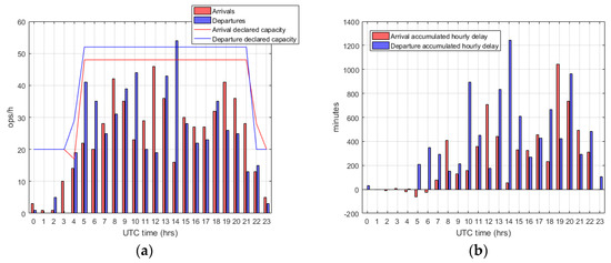
Figure 17.
(a) Traffic demand profile (22 July 2016) and (b) arrival/departure accumulated hourly delay profile (22 July 2016).
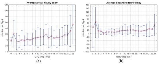
Figure 18.
Evolution of average hourly (a) arrival delay (min/operation); and (b) departure delay (min/operation) throughout the day (the error bars denote one standard deviation intervals).
Figure 17 shows that the arrival accumulated hourly delay presented two peak periods (11–13 and 19–21), with higher levels at the end of the day. Meanwhile, the departure delay rose as traffic demand reached capacity (near the hub operational windows). Moreover, Figure 18a illustrates that arrival average hourly delay increased and accumulated its impact over the day, due to the network effect. The departure delay (Figure 18b) did not completely follow the arrival delay patterns, which implies that the airport-airspace system is at times somehow capable of absorbing a fraction of the arrival delay across the rotation stage. We analysed this aptitude by studying three mutually exclusive and complementary stages: taxi-in, turnaround and taxi-out (Figure 19).
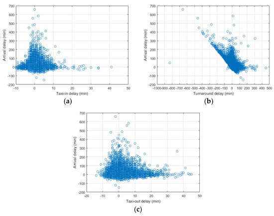
Figure 19.
Relationship between arrival delay and (a) taxi-in delay; (b) turnaround delay; and (c) taxi-out delay (min).
There was only a clear potential relationship between the arrival delay and time recovery in the case of the turnaround stage (Figure 19b). Unimpeded taxi times can only be as short as the physics of the process allows, but can grow large in the event of a slow taxi operation [17]. Therefore, the main opportunities to recover arrival delays arise at the turnaround stage. Moreover, as can be seen in Figure 20a, events of longer duration (arrival and turnaround) are the ones that contribute the most to departure delay, and therefore, to potential operational saturation of the airport. These stages are the most predisposed to generate delays, but also have greater possibility of recovery. Delay during taxiing processes does not reach large levels in absolute terms compared to other stages, but it can be relatively significant in situations of congestion or at certain times—at the beginning and end of the day for taxi-in and midday for taxi-out (Figure 20b).
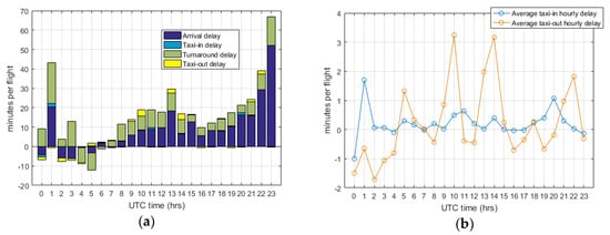
Figure 20.
(a) Contribution of each stage to departure hourly average delay (min/operation), and (b) evolution of average taxiing hourly delay (min/operation) throughout the day.
Figure 20a shows large positive delays at 1 UTC due to the sample size, which was limited for operations registered at this hour. The presence of several flights with an inherited reactionary lateness of more than 75 min has great impact on the average registered delay. Furthermore, these late inbound operations display turnaround inefficiencies that are related to the airport operational schedule overrun (aircraft landing and passengers disembarking at irregular hours, at sub-optimally allocated gates). However, these flights are particularly active in recovering time at the ASMA (additional ASMA 60 NM times are negative), helped by the fact that these are low congested hours. Arrival delays grow throughout the day due to the network effect; schedule adherence is achieved in the early hours of the day, but efficiency in handling the aircraft arrival flow is progressively degraded.
Figure 21a illustrates the system’s ability to absorb delay and recover schedule adherence through the “pure” turnaround stage (without considering ATFCM delay). We focused on medium-short delays (between +60 min and −60 min delay in arrival), since, for other thresholds, the relationship is not so illustrative (causes for long delays are more related to irregular operations than to inefficiencies). Figure 21b depicts this ability for the baseline day scenario.
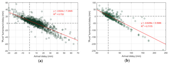
Figure 21.
Relationship between “pure” turnaround delay (without considering the ATFCM delay) and arrival delay, (a) for the complete dataset (only short delays) and (b) for the baseline day scenario (22 July 2016).
We found a strong negative correlation (R2 = 0.733) between the arrival delay and turnaround delay, which was statistically significant at the p = 0.02 level. The turnaround step is elastic enough to somehow adapt itself to arrival delay—when the arrival delay increased by 1 min, turnaround delay decreased by approximately by 0.8 min. The system responds to arrival delay through time buffers or by reducing operational times (improving efficiency), and hence, on ground turnaround partially absorbs the arrival delay. The elasticity of turnaround delay with respect to arrival delay depends on the type of operation (hour, airline, aircraft and route). Low cost carriers (LCCs) at midday hours and network carriers (NCs) with high scheduled turnaround times present the highest potential for recovery. Negative values in arrival delay usually result in positive turnaround delay values due to slot adherence (LEMD is a coordinated airport). Data do not demonstrate a clear positive relationship between delay (at the different stages) and the number of operations. Nevertheless, the correlation becomes stronger and statistically significant during congested hours (when the airport operates near its declared capacity). The elasticity of the “pure” turnaround delay with respect to arrival delay changes depends on the number of operations. Its threshold of less than 20 operations/h shows the higher potential for arrival delay recovery. Table 5 includes relevant information with respect to traffic mix and infrastructure utilization in order to better understand the discussion about the test cases results.
Table 5.
Relevant features regarding traffic mix and infrastructure utilization for the case study.
We analysed the operational pattern at the ATV stage through statistical characterization of the different processes that were previously identified with the BPM and the A-CDM milestone approach. The aim was to assess the amount of uncertainty in the system and its ability to “receive and transmit” aircraft flow with adherence to the expected schedule. Time efficiency performance was measured for each milestone (when scheduled and actual timestamps were available) or between two milestones (to assess the length of the process). We appraised the durations of processes, disturbances at their start/end times and delays. Table 6 illustrates the basic statistical data for the most relevant metrics. These data allowed us to characterise and model the processes (by fitting the duration or the starting time accuracy of the process to a statistical distribution) and derive performance indicators. Nevertheless, when designing optimal operational strategies, this average analysis should be adjusted to different clusters (types of fleets, airline operators, runway configurations, routes), as each of them presents different patterns. The influence of the different factors affecting time efficiency was addressed with the causal model (BN), and will be discussed in Section 4.2.
Table 6.
Statistical characterisation of the aircraft flow through the airspace/airside integrated operations.
When analysing flight delays, it should be noted that causes of short delays are often quite different from causes of long delays [7,100], which is why Figure 22 includes “sample outliers” (observations that are markedly different in value from the others of the sample). We define an outlier (for each metric) to be any observation outside the range [Q1 − k(Q3 − Q1), Q3 + k(Q3 − Q1)], with k = 1.5 [101], where Q1 and Q3 are the lower and upper quartiles respectively. The first quartile, denoted by Q1, is the median of the lower half of the dataset. This means that about 25% of the observations in the dataset lie below Q1 and about 75% lie above Q1. The third quartile, denoted by Q3, is the median of the upper half of the dataset. This means that about 75% of the observations in the dataset lie below Q3 and about 25% lie above Q3. During the analysis, these outliers (that could be due to faulty data or potential non-representative operations) might be excluded from the main sample, because of the possibility of biased results [they have an impact on the mean value (μ) and on the range (spread of data increases)]. Nevertheless, for items which are highly cantered at zero with wide variation (Figure 22), these outliers are important for the analysis, as they provide significant operational information.
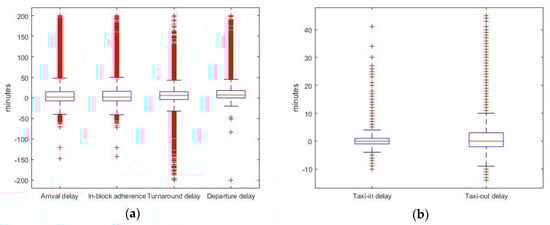
Figure 22.
Boxplot for (a) arrival delay, in-block adherence, turnaround delay and departure delay; and (b) taxi-in delay and taxi-out delay.
Figure 20, Figure 21 and Figure 22 consider negative values, which correspond to early schedule delays. Schedule delays (difference between a planned time and the actual time) are common occurrences in airline and airport operations, given the multiple agents involved, the stochastic nature of operating times, and the unexpected disruptions in tasks. “Negative” delays occur when the schedule is running close to plans and can cause issues for airport operations, e.g., disrupting the sequencing of flights and the allocation of resources (gates, handling equipment), especially during peak hours at busy airports [6]. “Positive” flight delays often cause significant problems for all the involved stakeholders, e.g., they affect the operational and financial performance of airports and airlines, schedule adherence and use of resources, passenger experience and satisfaction, and system reliability [2,6]. In our case study, data showed an increase in negative delays for the “pure” turnaround process at the following time frames: 4–6, 15–17 and 20–21. This corresponded to time efficiency recovery periods after the hub operational windows.
4.2. Cross-Influences at the ATV Stage
This section discusses the results that arose from the cross-influence analysis performed with the BN model. We aimed to understand how the diverse network layers that shape the BN structure (see Figure 14) affect the rest of interconnected nodes.
BNs have proven to be an excellent method to assess the airport operational saturation problem for different reasons: (a) their construction allows combination between data and expert knowledge/judgment; (b) inference can be performed efficiently in models with a large number of variables; (c) they develop a probabilistic approach to manage uncertainty and assess decision-making, which is consistent with the treatment of stochastic processes; (d) they allow cross-inference (several control variables) for deriving conclusions under uncertainty, where multiple sources of information and complex interaction patterns are involved; and (e) they are “white boxes”, in the sense that the model’s components (variables, links, probability and utility parameters) are open to interpretation, which makes it possible to perform a whole range of different analyses of the network (e.g., causal interactions, conflict analysis, (in)dependence analyses, sensitivity analysis, and value of information analysis).
The BN model allowed us to obtain valuable conclusions regarding uncertainty, delay and time saturation patterns (propagation dynamics, precursors and characteristics). Some of the lessons learned include information about the following:
- Main delay triggers and their quantitative influences, e.g., a high amount of arrivals at early hours of the day, congestion at ASMA and E-TMA, bad weather conditions, tight scheduled duration of processes, LCCs operating domestic flights, changes in runway configuration, departure rates approaching runway capacity, and the existence of external delay causes (traffic flow restrictions, aircraft technical problems, crew schedule adherence requisites).
- Ability of processes to compress themselves and achieve punctuality (potential for recovery), e.g., the overall turnaround delay decreases at a higher rate when the airport throughput is below the threshold of 20 operations/h, taxiing processes reduce their delay at certain runway configurations, longer scheduled turnarounds at midday and late evening act as time-efficiency “protectors” for the system, the unconstrained duration of airspace processes reaches a limit when the airport is operating near its declared capacity, and certain airlines are especially active in recovering arrival delay on the ground (reducing duration of processes).
The uncertainty of approach conditions makes traffic supply to runways a stochastic phenomenon. Hence, to ensure continuous traffic demand and maximise runway usage, a minimum level of queuing is required. Figure 23a illustrates the average landing rate (aircraft/h) as a function of the number of queuing aircraft at LEMD. It shows that the average landing rate stabilises once there are approximately 21 queuing aircraft and stays at around 40–41 aircraft/h. Therefore, any further approaches may lead to congestion and will not result in an improvement in the landing rate. Symmetrically, if we look at the departure process, the uncertainty of take-off conditions requires a minimum level of surface queuing to maximize runway usage. Pujet et al. [102] evaluated surface congestion by considering the take-off rate of an airport as a function of the number of aircraft taxiing out. Figure 23b depicts this relationship for LEMD, where the departure rate stabilizes at around 37–38 aircraft/h once there are approximately 36 departing aircraft on the ground (any further pushbacks may lead to congestion).
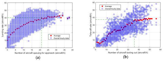
Figure 23.
(a) Average landing rate as a function of the number of queuing aircraft; and (b) average take-off rate as a function of the number of departing aircraft on the ground.
There is no stable relationship between the number of aircraft queuing at arrival and the runway departure rate per hour, beyond the fact that the two of them increase during peak hours. This means that, during the observation period, arrivals and departures were not limiting each other, apart from the declared capacity and the operational procedures. Nevertheless, during high delay periods, a cross-relationship was found that was statistically significant between arrival and departure processes, especially between the number of aircraft taxiing out and (a) the number of aircraft queuing for approach, (b) the number of flights with holding patterns and (c) the ASMA additional time.
Regarding airspace processes (E-TMA transit time, ASMA transit time and approach time), their durations during non-congested hours were rather inelastic with respect to arrival delay. Meanwhile, during congested hours, data showed a positive and statistically significant relationship between arrival delay and the number of aircraft queuing for landing, and between arrival delay and the number of flights with holding patterns. Therefore, the approach stage and its procedures proved to have substantial importance in reactionary delay and schedule adherence when the airport was operating near its declared capacity. Beyond the threshold of 20 arrivals/h, the arrival delay increased with the ASMA additional time, which, in turn, increased with the number of flights suffering holding patterns. The additional ASMA time and the number of flights with holding patterns almost stopped increasing when the landing rate reached 40 aircraft/h. This phenomenon is related to the airport’s arrival capacity limit.
As expected, bad weather conditions (high wind intensity and low visibility) had a considerable and statistically significant impact on delays, especially on those related to airspace processes, such as the E-TMA transit time, ASMA transit time and approach time. This conclusion also arose when separation between aircraft (measured at the Initial Approach Fix or at the runway threshold) significantly increased (over one standard deviation) above average values.
Regarding the influence of airport layout, the highest actual taxiing times resulted from the combination of north runway configuration and the use of the T123 terminal area and its associated stands. Conversely, the best opportunities for time-recovery at the taxiing stage (lowest taxiing delays) were found with the north configuration and the use of the T4/4S terminal area. Moreover, changes in runway configuration triggered an increment in actual taxiing times in the 30 min following the swift (delay was increased by 10%, on average). The runway configuration is associated with the dominant wind direction and the use of certain aircraft parking stands is related to the airline alliance that operates at each terminal area. Therefore, delay absorption strategies related to airport infrastructure use may not always be applicable. Nevertheless, our data showed that, within the same runway configuration, the use of different parallel runways could limit taxiing times (e.g., when T4T4S is assigned and the airport operates in north configuration, arrivals from runway 32R—and therefore, approaches coming from the east airspace suffer from a lower amount of taxi-in delays).
The quantitative influence of the different uncertainty sources was assessed by defining thresholds in the values of those variables that could cause a significant increase in the probability of having operational disruptions. Table 7 illustrates main departure delay precursors for each BN layer and their associated thresholds—when these conditions are reached, the probability of having a departure delay above 15 min is higher than 60%.
Table 7.
Most influential factors (and their thresholds) for departure delay propagation.
Regarding the predictive ability (forward scenario) of the causal model (BN), Figure 24 shows a comparison of real data and BN predicted outputs for the variable “departure delay”. For the real data histogram, we used a Kernel density estimation approach to obtain a nonparametric representation of the probability density function of the variable. As explained in Section 3.2.2., the errors for departure delay estimations had an average value of 10%.
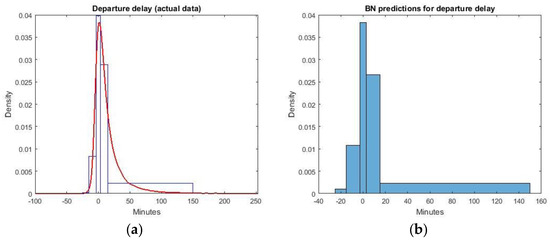
Figure 24.
Histograms for departure delay: (a) actual data; (b) BN predictions.
Moreover, the causal model (BN) allowed us to set different target levels for time efficiency and derive conclusions concerning the airport operation, e.g., by establishing different tolerable values regarding departure delay, we were able to discover issues related to operational strategies. Table 8 shows an example of backward inference in the BN model—for each departure delay state, it illustrates the most probable states (and their associated probabilities) regarding different variables. The node “departure delay” (node 42 in Figure 14) is discretized into five states (less than −15 min, −15 to −3 min, −3 to 3 min, 3 to 15 min and more than 15 min). The 15 min threshold for defining delay has historically been common to both Europe and the US [103,104,105] and the ±3 min threshold for punctuality was set by SESAR’s performance metrics [90].
Table 8.
Most probable states (and its associated probabilities) for different influence factors, when setting targets of operational time efficiency.
5. Summary and Conclusions
This paper developed an overview of the operations that represent aircraft flow through an airspace/airside system. In this analysis, we used a dynamic spatial boundary associated with the E-TMA concept, so that a linkage between inbound and outbound flights could be proposed. The aircraft flow was characterised by several temporal milestones related to the A-CDM method and structured by a hieratical task analysis, providing a BPM for the ATV stage.
The application of the methodology to a case study of 34,000 turnarounds (registered at the peak months of 2016) at Madrid Airport showed that arrival delay increases and accumulates its impact over the day, due to network effects. However, departure delay does not follow this pattern, which implies that the airspace/airside system is somehow capable of absorbing a fraction of the arrival delay across the ATV stage. We analysed this aptitude by studying and characterising the different processes that were previously identified with the BPM and the milestone approach. This evaluation of the system’s dynamics was completed with an appraisal of the relationships between the factors that influence the aircraft flow. We created a probabilistic graphical model, using a Bayesian Network approach that managed uncertainty at the ATV stage. It predicted outbound delays given the probability of having different values of the causal control variables. Moreover, by setting a target to the output delay, the model provided the optimal configuration for the input nodes. Different lessons can be learned regarding uncertainty propagation, time saturation and system recovery (where to act). The main potential drivers for delay include the time of the day, congestion at ASMA, weather conditions, amount of arrival delay, scheduled duration of processes, runway configuration, airline business model, handling agent, aircraft type, route origin/destination and existence of ATFCM regulations. Events of longer duration (arrival and turnaround) are the ones that contribute the most to departure delay, but are also those where more possibilities for recovery exist. In that sense, the model also informs us about how sensitive the different processes are to changes in arrival delay (arrival delay elasticity of processes). The proposed methodology has several applications. It can
- Achieve a comprehensive understanding of operations at the ATV stage (airspace/airside integration).
- Appraise the influence of changes in tactical decisions and policies on delay management (“what-if” scenarios).
- Ensure some target levels of efficiency are met, improve predictability and manage uncertainty regarding operations through the causal model.
- Estimate the final departure delay (settlement of buffer time and optimal rotation times) using “forward” analysis.
- Identify the main contributors (causes) to a final delay (locate inefficiencies) using “backward” analysis.
These applications address several challenges of the airport/airline industry—enhancing the system’s efficiency, improving robustness in the presence of operational uncertainties, easing resource allocation with multiple stakeholders and developing a decision-support tool that accounts for delay dynamics and behaviour. Future work will be focused on improving the accuracy and reliability of the model (more complete testing data and methodological improvements) and on comparing the results when the methodology is applied to other airports (generalise the case study). We also need to analyse potential response strategies/measures (reduce delays, mitigate inefficiencies and optimise operations), and apply the propagation model to other types of incidents (not just delays).
Author Contributions
A.R.-S. conceived and wrote the paper, and conducted the final editing; A.R.-S., F.G.C. and R.A.V. developed the methodology, analysed the data and structured the results; J.M.C.G. provided the data, supervised the results and reviewed the content; M.B. contributed to methodological improvements and reviewed the results; F.G.C. and R.A.V. supervised the conclusions.
Acknowledgments
We would like to thank the editors and the anonymous reviewers for their careful reading of our manuscript and their insightful comments and suggestions. We believe that the quality of the manuscript has been significantly improved as a result.
Conflicts of Interest
The authors declare no conflict of interest.
References
- Goedeking, P. Networks in Aviation: Strategies and Structures; Springer: Berlin/Heidelberg, Germany, 2010. [Google Scholar]
- Belobaba, P.; Odoni, A.; Barnhart, C. The Global Airline Industry, 2nd ed.; John Wiley & Sons, Ltd.: New York, NY, USA, 2015. [Google Scholar]
- Ashford, N.J.; Stanton, H.P.M.; Moore, C.A.; Coutu, P.; Beasley, J.R. Airport Operations, 3rd ed.; McGraw-Hill: New York, NY, USA, 2013. [Google Scholar]
- Janić, M. The flow management problem in air traffic control: A model of assigning priorities for landings at a congested airport. Transp. Plan. Technol. 1997, 20, 131–162. [Google Scholar] [CrossRef]
- Beatty, R.; Hsu, R.; Berry, L.; Rome, J. Preliminary Evaluation of Flight Delay Propagation through an Airline Schedule. Air Traffic Control Q. 1999, 7, 259–270. [Google Scholar] [CrossRef]
- Wu, C.L. Airline Operations and Delay Management: Insights from Airline Economics, Networks and Strategic Schedule Planning, 1st ed.; Ashgate Publishing: Surrey, UK, 2012. [Google Scholar]
- Wu, C.L. Inherent delays and operational reliability of airline schedules. J. Air Transp. Manag. 2005, 11, 273–282. [Google Scholar] [CrossRef]
- Pyrgiotis, N.; Malone, K.M.; Odoni, A. Modelling delay propagation within an airport network. Transp. Res. Part C Emerg. Technol. 2013, 27, 60–75. [Google Scholar] [CrossRef]
- SESAR. SESAR Concept of Operations Step 2 Edition 2014 (Ed. 01.01.00); SESAR Joint Undertaking: Brussels, Belgium, 2014. [Google Scholar]
- Kazda, A.; Caves, R.E. Airport Design and Operations, 2nd ed.; Elsevier: Amsterdam, The Netherlands, 2007. [Google Scholar]
- Zellweger, A.G.; Donohue, G.L. Air Transportation Systems Engineering, 1st ed.; American Institute of Aeronautics and Astronautics (AIAA): Reston, VA, USA, 2001. [Google Scholar]
- ICAO. Doc 9854: Global Air Traffic Management Operational Concept; International Aviation Civil Organization: Montreal, QC, Canada, 2005. [Google Scholar]
- SESAR. European ATM Master Plan—Edition 2015; Publications Office of the European Union: Luxembourg, 2015. [Google Scholar]
- FAA. The Future of the NAS, Washington D.C: U.S. Department of Transportation, Federal Aviation Administration, Office of NextGen. 2016. Available online: https://www.faa.gov/nextgen/media/futureofthenas.pdf (accessed on 16 January 2018).
- Wu, C.L.; Caves, R.E. Modelling and simulation of aircraft turnaround operations at airports. Transp. Plan. Technol. 2004, 27, 25–46. [Google Scholar] [CrossRef]
- Cook, A. European Air Traffic Management: Principles, Practice and Research, 1st ed.; Ashgate: Aldershot, UK, 2007. [Google Scholar]
- Simaiakis, I.; Balakrishnan, H. A Queuing Model of the Airport Departure Process. Transp. Sci. 2015, 50, 94–109. [Google Scholar] [CrossRef]
- Neyshabouri, S.; Sherry, L. Analysis of Airport Surface Operations: A Case-Study of Atlanta Hartfield Airport. In Proceedings of the Transportation Research Board 93rd Annual Meeting, Washington, DC, USA, 12–16 January 2014. [Google Scholar]
- Zografos, K.G.; Andreatta, G.; Odoni, A.R. Modelling and Managing Airport Performance; Wiley & Sons: Chichester, UK, 2013. [Google Scholar]
- Dobruszkes, F.; Givoni, M.; Vowles, T. Hello major airports, goodbye regional airports? Recent changes in European and US low-cost airline airport choice. J. Air Transp. Manag. 2017, 59, 50–62. [Google Scholar] [CrossRef]
- Fageda, X.; Flores-Fillol, R. How do airlines react to airport congestion? The role of networks. Reg. Sci. Urban Econ. 2016, 56, 73–81. [Google Scholar] [CrossRef]
- Redondi, R.; Gudmundsson, S.V. Congestion spill effects of Heathrow and Frankfurt airports on connection traffic in European and Gulf hub airports. Transp. Res. Part A Policy Pract. 2016, 92, 287–297. [Google Scholar] [CrossRef]
- Suau-Sanchez, P.; Voltes-Dorta, A.; Rodríguez-Déniz, H. Measuring the potential for self-connectivity in global air transport markets: Implications for airports and airlines. J. Transp. Geogr. 2016, 57, 70–82. [Google Scholar] [CrossRef]
- Wu, C.L. Monitoring Aircraft Turnaround Operations—Framework Development, Application and Implications for Airline Operations. Transp. Plan. Technol. 2008, 31, 215–228. [Google Scholar] [CrossRef]
- Filar, J.A.; Manyem, P.; White, K. How Airlines and Airports Recover from Schedule Perturbations: A Survey. Ann. Oper. Res. 2001, 108, 315–333. [Google Scholar] [CrossRef]
- Mukherjee, A.; Hansen, M.; Grabbe, S. Ground delay program planning under uncertainty in airport capacity. Transp. Plan. Technol. 2012, 35, 611–628. [Google Scholar] [CrossRef]
- Ciruelos, C.; Arranz, A.; Etxebarria, I.; Peces, S. Modelling Delay Propagation Trees for Scheduled Flights. In Proceedings of the 11th USA/EUROPE Air Traffic Management R&D Seminar, Lisbon, Portugal, 23–26 June 2015. [Google Scholar]
- Cook, A.; Tanner, G.; Cristobal, S.; Zanini, M. Delay propagation: New metrics, new insights. In Proceedings of the 11th USA/EUROPE Air Traffic Management R&D Seminar, Lisbon, Portugal, 23–26 June 2015. [Google Scholar]
- Campanelli, B.; Fleurquin, P.; Eguíluz, V.M.; Ramasco, J.J.; Arranz, A.; Etxebarría, I.; Ciruelos, C. Modeling Reactionary Delays in the European Air Transport. In Proceedings of the 4th SESAR Innovation Days, Madrid, Spain, 26 November 2014. [Google Scholar]
- Rebollo, J.J.; Balakrishnan, H. Characterization and prediction of air traffic delays. Transp. Res. Part C Emerg. Technol. 2014, 44, 231–241. [Google Scholar] [CrossRef]
- Gopalakrishnan, K.; Balakrishnan, H.; Jordan, R. Deconstructing Delay Dynamics: An Air Traffic Delay Example. In Proceedings of the International Conference on Research in Air Transportation, Philadelphia, PA, USA, 20–24 June 2016. [Google Scholar]
- Fricke, H.; Schultz, M. Delay impacts onto turnaround performance. In Proceedings of the 8th USA/Europe Air Traffic Management Research and Development Semina, Napa, CA, USA, 29 June–2 July 2009. [Google Scholar]
- Katsaros, A.; Sánchez, A.C.S.; Zerkowitz, S.; Kerulo, B.; Stark, N.; Rekiel, J.; Pascual, S.P. Limiting the impact of aircraft turnaround inefficiencies on airport and network operations: The TITAN project. J. Airpt. Manag. 2013, 7, 289–317. [Google Scholar]
- Oreschko, B.; Kunze, T.; Gerbothe, T.; Fricke, H. Turnaround prediction and controling with micrsocopic process modelling GMAN proof of concept & possiblities to use microscopic process szenarios as control options. In Proceedings of the 6th International Conference on Research in Air Transportation, Istanbul, Turkey, 26–30 May 2014. [Google Scholar]
- Eurocontrol. A-CDM Impact Assessment; European Organisation for the Safety of Air Navigation: Brussels, Belgium, 2016. [Google Scholar]
- Schmitt, D.; Gollnick, V. Air Transport System, 1st ed.; Springer: Wien, Austria, 2016. [Google Scholar]
- Daley, B. Air Transport and the Environment, 1st ed.; Routledge: Abington-on-Thames, UK, 2010. [Google Scholar]
- Cook, A.; Tanner, G. European Airline Delay Cost Reference; University of Westminster Comissioned by Eurocontrol Performance Review Unit: Brussels, Belgium, 2014. [Google Scholar]
- Bazargan, M. Airline Operations and Scheduling, 2nd ed.; Ashgate: Aldershot, UK, 2010. [Google Scholar]
- Marintseva, K.; Yun, G.; Kachur, S. Resource allocation improvement in the tasks of airport ground handling operations. Aviation 2015, 19, 7–13. [Google Scholar] [CrossRef]
- Norin, A.; Granberg, T.A.; Yuan, D.; Värbrand, P. Airport logistics—A case study of the turn-around process. J. Air Transp. Manag. 2012, 20, 31–34. [Google Scholar] [CrossRef]
- Wang, P.T.R.; Schaefer, L.; Wojcik, L.A. Flight connections and their impacts on delay propagation. In Proceedings of the 22nd Digital Avionics Systems Conference, Indianapolis, IN, USA, 12–16 October 2003. [Google Scholar]
- Tu, Y.; Ball, M.O.; Jank, W.S. Estimating Flight Departure Delay Distributions—A Statistical Approach with Long-Term Trend and Short-Term Pattern. J. Am. Stat. Assoc. 2008, 103, 112–125. [Google Scholar] [CrossRef]
- AhmadBeygi, S.; Cohn, A.; Guan, Y.; Belobaba, P. Analysis of the potential for delay propagation in passenger airline networks. J. Air Transp. Manag. 2008, 14, 221–236. [Google Scholar] [CrossRef]
- Fleurquin, P.; Campanelli, B.; Eguíluz, V.M.; Ramasco, J.J. Trees of Reactionary Delay: Addressing the Dynamical Robustness of the US Air Transportation Network. In Proceedings of the 4th SESAR Innovation Days, Madrid, Spain, 25–27 November 2014. [Google Scholar]
- Abdel-Aty, M.; Lee, C.; Bai, Y.; Li, X.; Michalak, M. Detecting periodic patterns of arrival delay. J. Air Transp. Manag. 2007, 13, 355–361. [Google Scholar] [CrossRef]
- Wong, J.T.; Tsai, S.C. A survival model for flight delay propagation. J. Air Transp. Manag. 2012, 23, 5–11. [Google Scholar] [CrossRef]
- Churchill, A.; Lovell, D.; Ball, M. Examining the temporal evolution of propagated delays at individual airports: Case studies. In Proceedings of the 7th USA/Europe Air Traffic Management Research Devlopment Seminar, Barcelona, Spain, 2–5 July 2007. [Google Scholar]
- Deutschmann, A. Prediction of airport delays based on non-linear considerations of airport systems. In Proceedings of the 28th Congress of the International Council of the Aeronautical Sciences, Brisbane, Australia, 23–28 September 2012. [Google Scholar]
- Belkoura, S.; Zanin, M. Phase changes in delay propagation networks. In Proceedings of the 7th the International Conference for Research in Air Transportation, Philadelphia, PA, USA, 20–24 June 2016. [Google Scholar]
- Pearl, J. Fusion, propagation, and structuring in belief networks. Artif. Intell. 1986, 29, 241–288. [Google Scholar] [CrossRef]
- Pearl, J. Belief networks revisited. Artif. Intell. 1993, 59, 49–56. [Google Scholar] [CrossRef]
- Fenton, N.; Neil, M. Risk Assessment and Decision Analysis with Bayesian Networks; CRC Press: Boca Raton, FL, USA, 2013. [Google Scholar]
- Koller, D.; Friedman, N. Probabilistic Graphical Models: Principles and Techniques, 1st ed.; The MIT Press: Cambridge, UK, 2011. [Google Scholar]
- Bujor, A.; Ranieri, A. Assessing Air Traffic Management Performance Interdependencies through Bayesian Networks: Preliminary Applications and Results. J. Traffic Transp. Eng. 2016, 4, 34–48. [Google Scholar] [CrossRef]
- Farr, A.C.; Kleinschmidt, T.; Johnson, S.; Yarlagadda, P.K.D.V.; Mengersen, K.L. Investigating effective wayfinding in airports: A Bayesian network approach. Transport 2013, 90–99. [Google Scholar] [CrossRef]
- Laskey, K.B.; Xu, N.; Chen, C.H. Propagation of delays in the national airspace system. In Proceedings of the 22nd Conference in Uncertainty in Artificial Intelligence, Cambridge, MA, USA, 13–16 July 2006. [Google Scholar]
- Xu, N.; Donohue, G.; Laskey, K.B.; Chen, C. Estimation of delay propagation in the national aviation system using bayesian networks. In Proceedings of the 6th USA/Europe Air Traffic Management Research and Development Semina, Baltimore, MD, USA, 27–30 June 2005. [Google Scholar]
- Liu, Y.; Wu, H. A Remixed Bayesian Network Based Algorithm for Flight Delay Estimating. Int. J. Pure Appl. Math. 2013, 85, 465–475. [Google Scholar] [CrossRef]
- Morales-Napoles, O.; Hanea, A.; Kurowicka, D.; Cooke, R.M.; Roelen, A. Causal modelling in the Aviation Industry: An application for controlled flight into terrain. In Safety Reliability Management Risk; Guedes, C., Soares, E.Z., Eds.; Taylor & Francis: London, UK, 2006; pp. 1831–1838. [Google Scholar]
- Londner, E.H.; Moss, R.J. A Bayesian Network Model of Pilot Response to TCAS Resolution Advisories. In Proceedings of the 12th USA/Europe Air Traffic Management R&D Seminar, Seattle, WA, USA, 27–30 June 2017. [Google Scholar]
- Yorukoglu, M.; Kayakutlu, G. Bayesian Network Scenarios to improve the Aviation Supply Chain. In Proceedings of the World Congress on Engineering, London, UK, 6–8 July 2011; Volume 2. [Google Scholar]
- Buldyrev, S.V.; Parshani, R.; Paul, G.; Stanley, H.E.; Havlin, S. Catastrophic cascade of failures in interdependent networks. Nature 2010, 464, 1025–1028. [Google Scholar] [CrossRef] [PubMed]
- Liu, Y.-J.; Ma, S. Flight Delay and Delay Propagation Analysis Based on Bayesian Network. In Proceedings of the 2008 Knowledge Acquisition and Modeling, Wuhan, China, 21–22 December 2008; pp. 318–322. [Google Scholar]
- Zio, E.; Sansavini, G. Modeling interdependent network systems for identifying cascade-safe operating margins. IEEE Trans. Reliab. 2011, 60, 94–101. [Google Scholar] [CrossRef]
- Liu, Y.-J.; Cao, W.-D.; Ma, S. Estimation of Arrival Flight Delay and Delay Propagation in a Busy Hub-Airport. In Proceedings of the 4th International Conference on Natural Computation, Jinan, China, 18–20 October 2008. [Google Scholar]
- Schaefer, L.; Noam, T. Aircraft Turnaround Times for Air Traffic Simulation Analyses. In Proceedings of the Transportation Research Board 82nd Annual Meeting Compendium of Papers CD-ROM, Washington DC, USA, 12–16 January 2003. [Google Scholar]
- Eurocontrol, ACI, IATA. Airport CDM Implementation: The Manual; European Organisation for the Safety of Air Navigation: Brussels, Belgium, 2012. [Google Scholar]
- Bagieu, S. SESAR Solution Development, Unpacking SESAR Solutions, Extended AMAN; SESAR Joint Undertaking Solutions Workshop: Paris, France, 2015. [Google Scholar]
- Wilke, S.; Majumdar, A.; Ochieng, W.Y. Airport surface operations: A holistic framework for operations modeling and risk management. Saf. Sci. 2014, 63, 18–33. [Google Scholar] [CrossRef]
- Kirwan, B.; Ainsworth, L.K. A Guide To Task Analysis: The Task Analysis Working Group, 1st ed.; Taylor & Francis: London, UK, 1992. [Google Scholar]
- IBERIA. Flight Operations Manuals; IBERIA: Madrid, Spain, 2015. [Google Scholar]
- IBERIA. Ground Handling Operations Manuals; IBERIA: Madrid, Spain, 2014. [Google Scholar]
- IATA. Airport Handling Manual, 35th ed.; International Air Transport Association: Montreal, QC, Canada, 2015. [Google Scholar]
- ICAO. Annex 14 to the Convention on International Civil Aviation, Volume 1: Aerodrome Design and Operations, 7th ed.; International Aviationl Civil Organization: Montreal, QC, Canada, 2016. [Google Scholar]
- ICAO. Document 9157: Aerodrome Design Manual, 3rd ed.; International Civil Aviation Organization: Montreal, QC, Canada, 2006. [Google Scholar]
- ICAO. Document 8168: Procedures for Air Navigation Services—Aircraft Operations, 5th ed.; International Civil Aviation Organization: Montreal, QC, Canada, 2006. [Google Scholar]
- ICAO. Safety Oversight Manual—Part A, 2nd ed.; International Civil Aviation Organization: Montreal, QC, Canada, 2006. [Google Scholar]
- Engels, G.; Förster, A.; Heckel, R.; Thöne, S. Process modeling using UML. In Process-Aware Information Systems: Bridging People and Software Through Process Technology, 1st ed.; Dumas, M., van der Aalst, W.M.P., Hofstede, A.H.M.T., Eds.; Wiley & Sons: Chichester, UK, 2005; pp. 85–118. [Google Scholar]
- Carlier, S.; de L´epinay, I.; Hustache, J.; Jelinke, F. Environmental impact of air traffic flow management delays. In Proceedings of the 7th USA/Europe Air Traffic Management Research and Development, Barcelona, Spain, 2–5 July 2007. [Google Scholar]
- ENAIRE, Aeronautical Information Publication (AIP). Aeronautical Information Service (AIS). 2018. Available online: https://ais.enaire.es/aip/aipcd_en.aspx (accessed on 16 January 2018).
- Rakas, J. Defining and Measuring Aircraft Delay and Airport Capacity Thresholds; Airport Cooperative Research Program (ACRP) Report 104; Transportation Research Board (TRB): Washington, DC, USA, 2014. [Google Scholar]
- Garson, G.D. Curve Fitting and Nonlinear Regression; Statistical Associates Publishers: Asheboro, NC, USA, 2012. [Google Scholar]
- Scott, D.W. Multivariate Density Estimation: Theory, Practice, and Visualization, 2nd ed.; Wiley & Sons: New York, NY, USA, 2015. [Google Scholar]
- Kjærulff, U.B.; Madsen, A.L. Bayesian Networks and Influence Diagrams—A Guide to Construction and Analysis, 2nd ed.; Springer: New York, NY, USA, 2013. [Google Scholar]
- Darwiche, A. Bayesian networks. Commun. ACM 2010, 53, 80–90. [Google Scholar] [CrossRef]
- Neapolitan, R.E. Learning Bayesian Networks, 1st ed.; Prentice Hall: Upper Saddle River, NJ, USA, 2003. [Google Scholar]
- Nielsen, T.D.; Jensen, F.V. Bayesian Network and Decision Graph; Springer: New York, NY, USA, 2007. [Google Scholar]
- Pearl, J. Causality, 2nd ed.; Cambridge University Press: New York, NY, USA, 2009. [Google Scholar]
- Cook, A.; Tanner, G.; Zannin, M. Towards superior air transport performance metrics—Imperatives and methods. J. Aerosp. Oper. 2013, 2, 3–19. [Google Scholar] [CrossRef]
- GeNIe Modeler, version 2.2; BayesFusion, LLC: Pittsburgh, PA, USA, 2017.
- Cooper, G.F.; Herskovits, E. A bayesian method for the induction of probabilistic networks from data. Mach. Learn. 1992, 9, 309–347. [Google Scholar] [CrossRef]
- Heckerman, D.; Geiger, D.; Chickering, D.M. Learning Bayesian Networks: The Combination of Knowledge and Statistical Data. Mach. Learn. 1995, 20, 197–243. [Google Scholar] [CrossRef]
- Suzuki, J. A Theoretical Analysis of the BDeu Scores in Bayesian Network Structure Learning. Behaviormetrika 2017, 44, 97–116. [Google Scholar] [CrossRef]
- Koiter, J.R. Visualizing Inference in Bayesian Networks, PhD Thesis in the Faculty of Electrical Engineering, Mathematics, and Computer Science; Department of Man-Machine Interaction, Delft University of Technology: Delft, The Netherlands, 2006. [Google Scholar]
- Hastie, T.; Tibshirani, R.; Friedman, J. The Elements of Statistical Learning; Springer: New York, NY, USA, 2009. [Google Scholar]
- Fawcett, T. An introduction to ROC analysis. Pattern Recognit. Lett. 2006, 27, 861–874. [Google Scholar] [CrossRef]
- IATA. Airport Development Reference Manual, 10th ed.; International Air Transport Association: Montreal, QC, Canada, 2016. [Google Scholar]
- ICAO. Document 8643: Aircraft Type Designators; International Civil Aviation Organization: Montreal, QC, Canada, 2016. [Google Scholar]
- EUROCONTROL, CODA (Central Office for Delay Analysis) Digest: All-Causes Delay and Cancellations to Air Transport in Europe—2016; European Organisation for the Safety of Air Navigation: Brussels, Belgium, 2017.
- Tukey, J.W. Exploratory Data Analysis, 1st ed.; Pearson: London, UK, 1977. [Google Scholar]
- Pujet, N.; Delcaire, B.; Feron, E. Input-Output Modeling and Control of the Departure Process of Busy Airports. Air Traffic Control Q. 2000, 8, 1–32. [Google Scholar] [CrossRef]
- Cook, A.; Tanner, G.; Cristóbal, S.; Zanin, M. Passenger-Oriented Enhanced Metrics. In Proceedings of the 2nd SESAR Innovation Days, Braunschweig, Germany, 28 November 2012. [Google Scholar]
- Jetzki, M. The Propagation of Air Transport Delays in Europe. Ph.D. Thesis, Department of Airport and Air Transportation Research, RWTH Aachen University, Aachen, Germany, 2009. [Google Scholar]
- Sherry, L.; Wang, D.; Xu, N.; Larson, M.; Sherry, L.; Xu, N.; Larson, M. Statistical Comparison of Passenger Trip Delay and Flight Delay Metrics. J. Chem. Inf. Model. 2013, 53, 1689–1699. [Google Scholar] [CrossRef]


© 2018 by the authors. Licensee MDPI, Basel, Switzerland. This article is an open access article distributed under the terms and conditions of the Creative Commons Attribution (CC BY) license (http://creativecommons.org/licenses/by/4.0/).