Aircraft Geometry and Meshing with Common Language Schema CPACS for Variable-Fidelity MDO Applications


Abstract
:1. Introduction
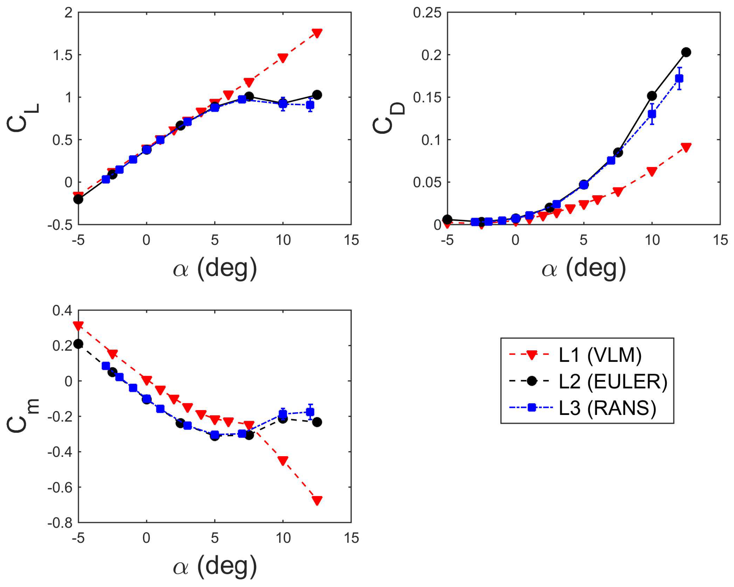
- L0:
- handbook methods, based on statistics and/or empirical design rules;
- L1:
- based on simplified physics, can model and capture a limited amount of effects. For example, the linearized-equation models, the Vortex-Lattice Method (VLM) or the panel method in aerodynamics;
- L2:
- based on accurate physics representations. For example, the non-linear analysis, Euler-based CFD;
- L3:
- represents the highest end simulations, usually used to capture detailed local effects, but do not allow wide exploration of the design space due to computational cost. Additionally, the modeling may require extensive ad hoc manual intervention. For example, the highest fidelity methods, RANS-based CFD.
1.1. Background
1.2. Aerodynamic Model Description
2. CPACS File Description
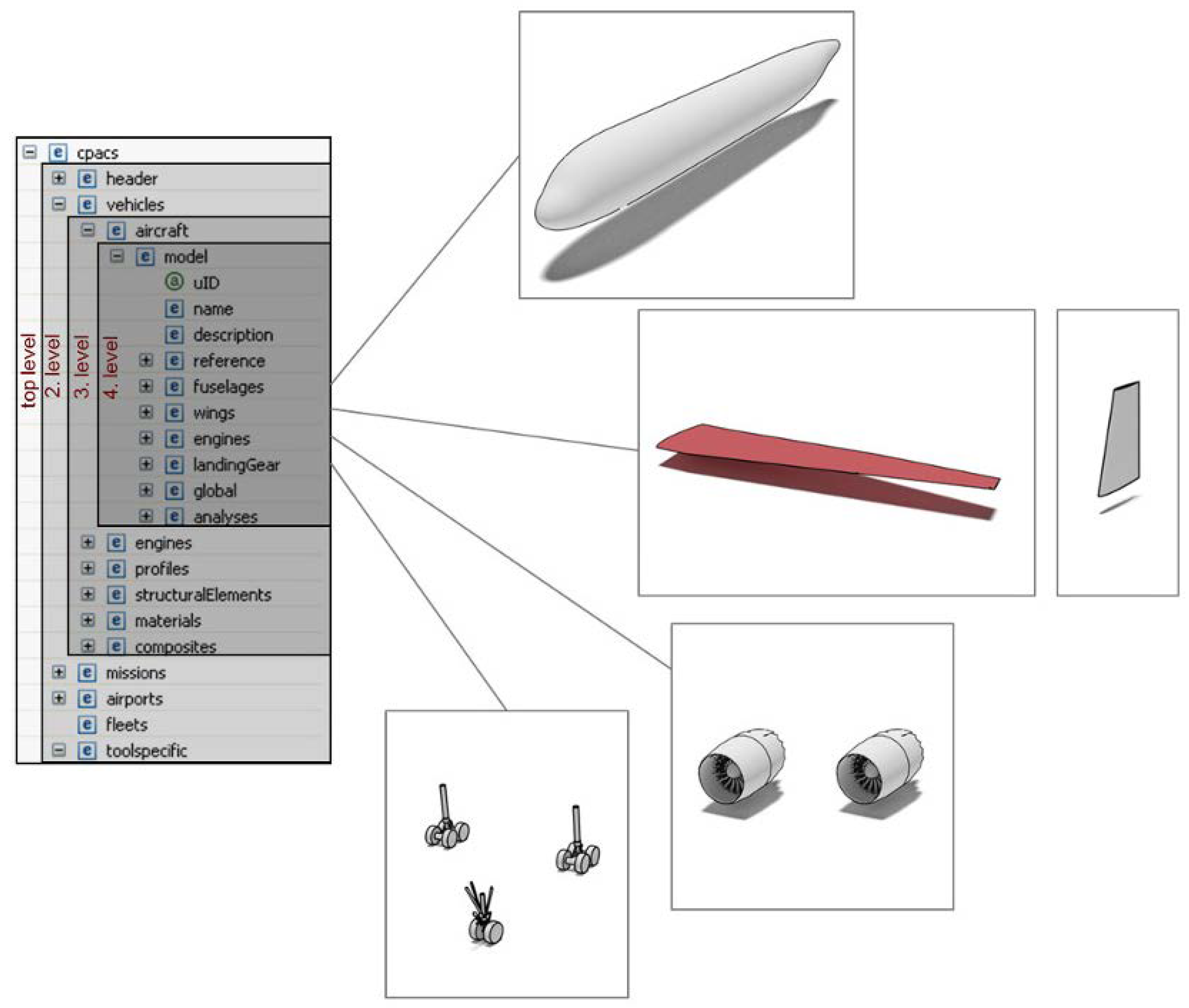
2.1. The CPACS Hierarchical Data Definition Structure
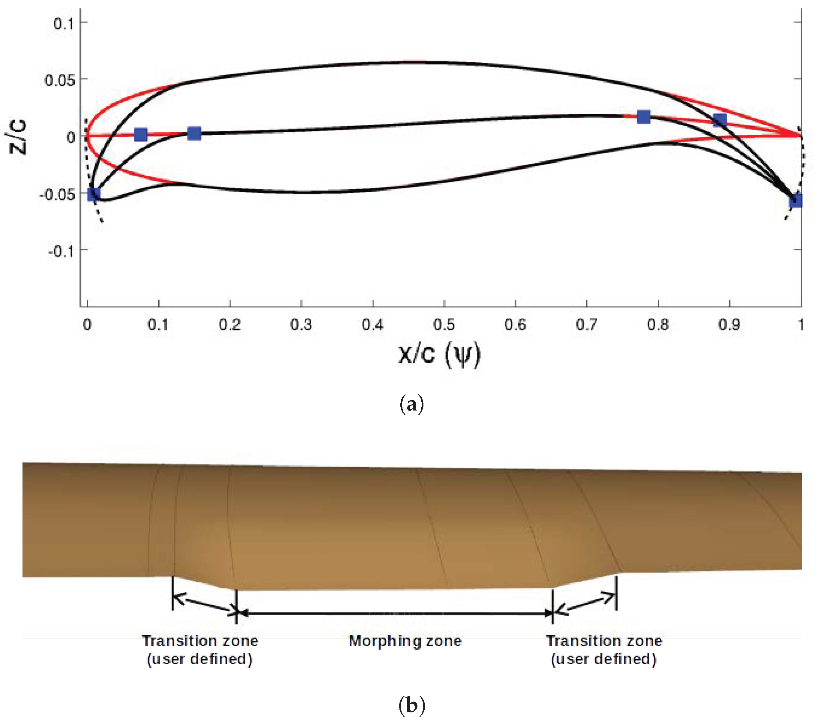
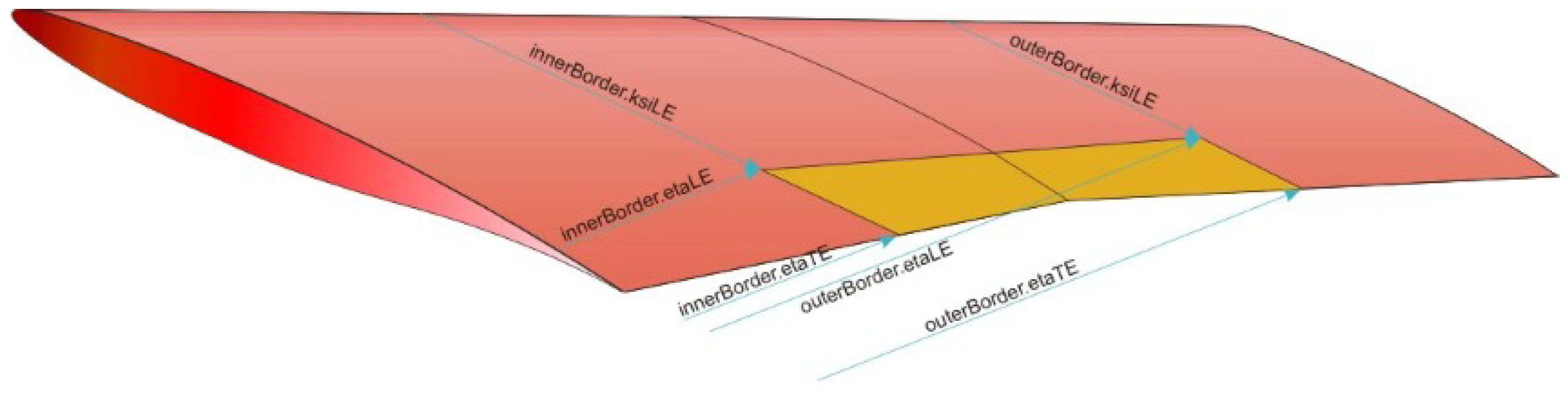
2.2. The CPACS Control Surface Definition
3. Geometry and CPACS Interfaces for Variable Fidelity Tools
3.1. CPACS-Tornado Interface
- Aircraft configuration visualization including fuselage representation and control surface identifications;
- Fast MEX-compiled version of core-functions for matrix computations;
- All-moving surfaces and overlapped movable surfaces.
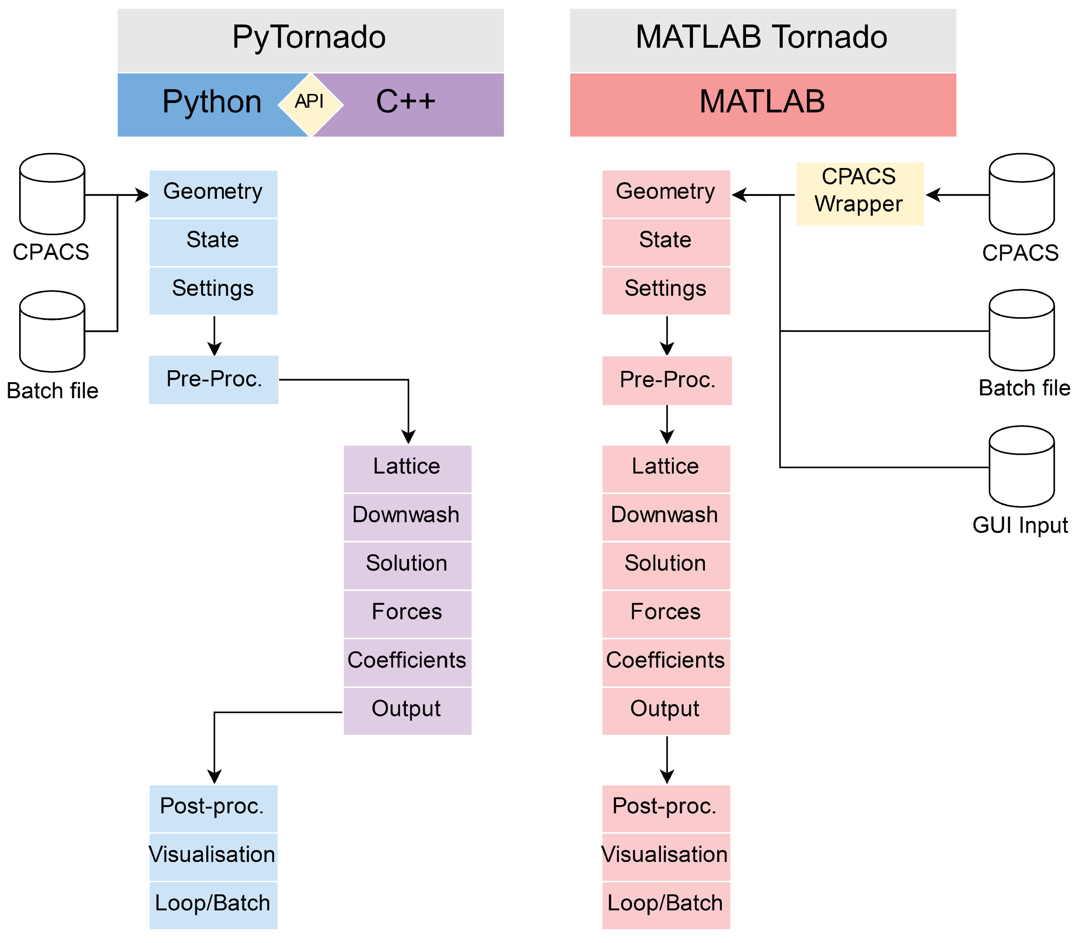
PyTornado: A VLM Solver with Native CPACS Compatibility
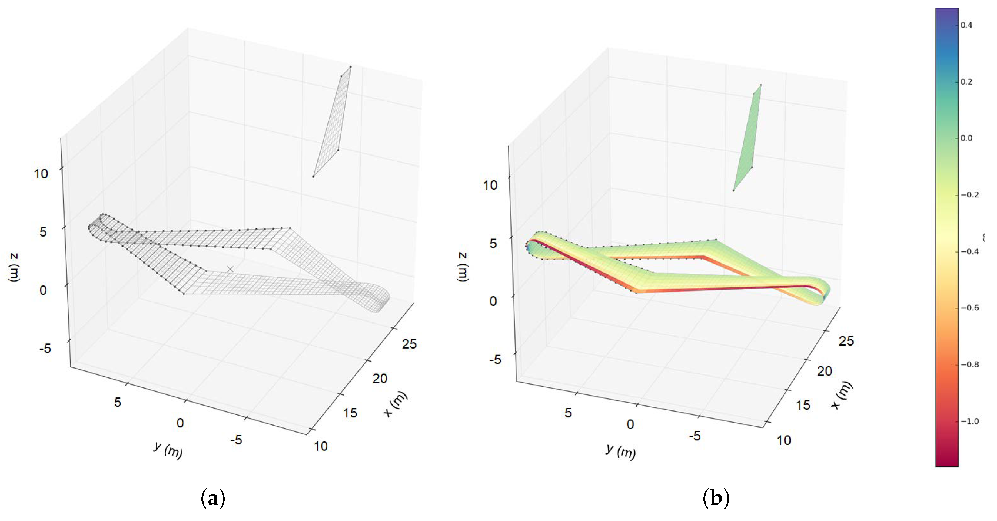
- A Python wrapper, dedicated to high-level tasks such as communication with CPACS, pre- and post-processing for VLM, as well as visualization of the model and generated results; see Figure 7a,b,
- The actual VLM solver, re-structured and re-written in C++ from the MATLAB Tornado VLM solver with performance in mind.
3.2. CPACS-Sumo Interface
3.2.1. Sumo: A Gateway from CPACS to Higher-Fidelity Aerodynamics
3.2.2. The Interface CPACS2SUMO
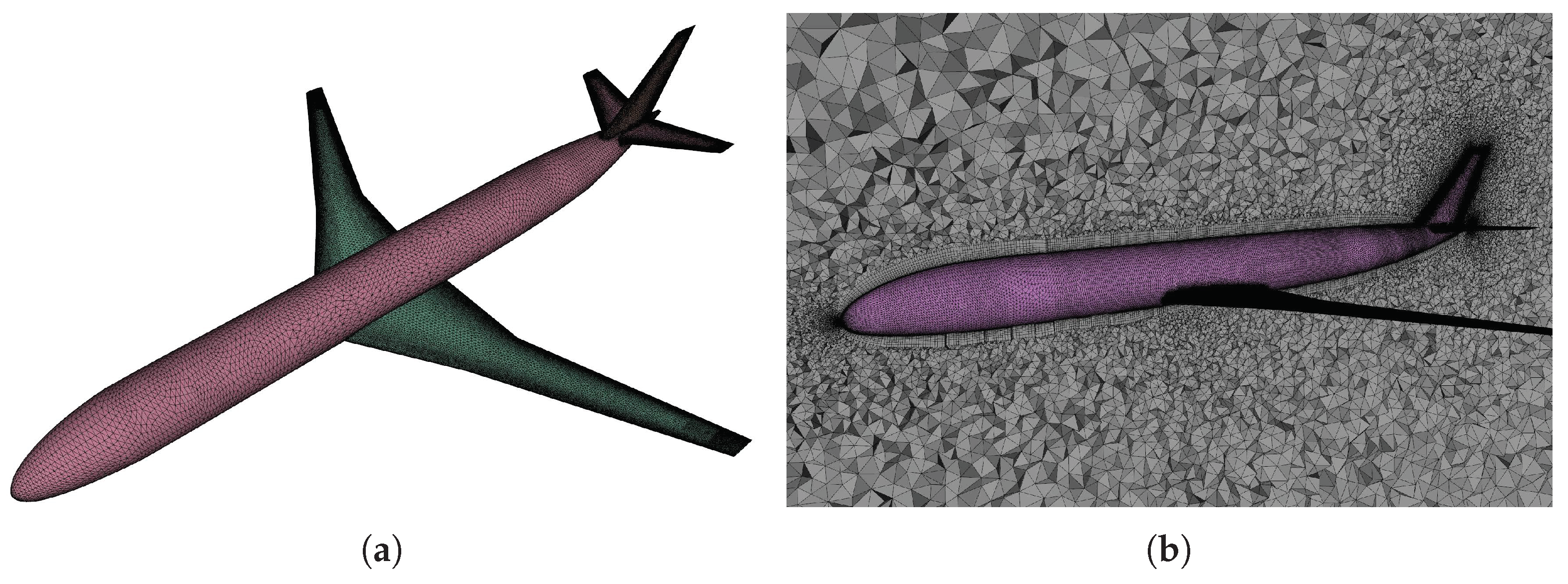
4. Flow Solvers
5. Applications
5.1. Aerodynamic Results Comparison
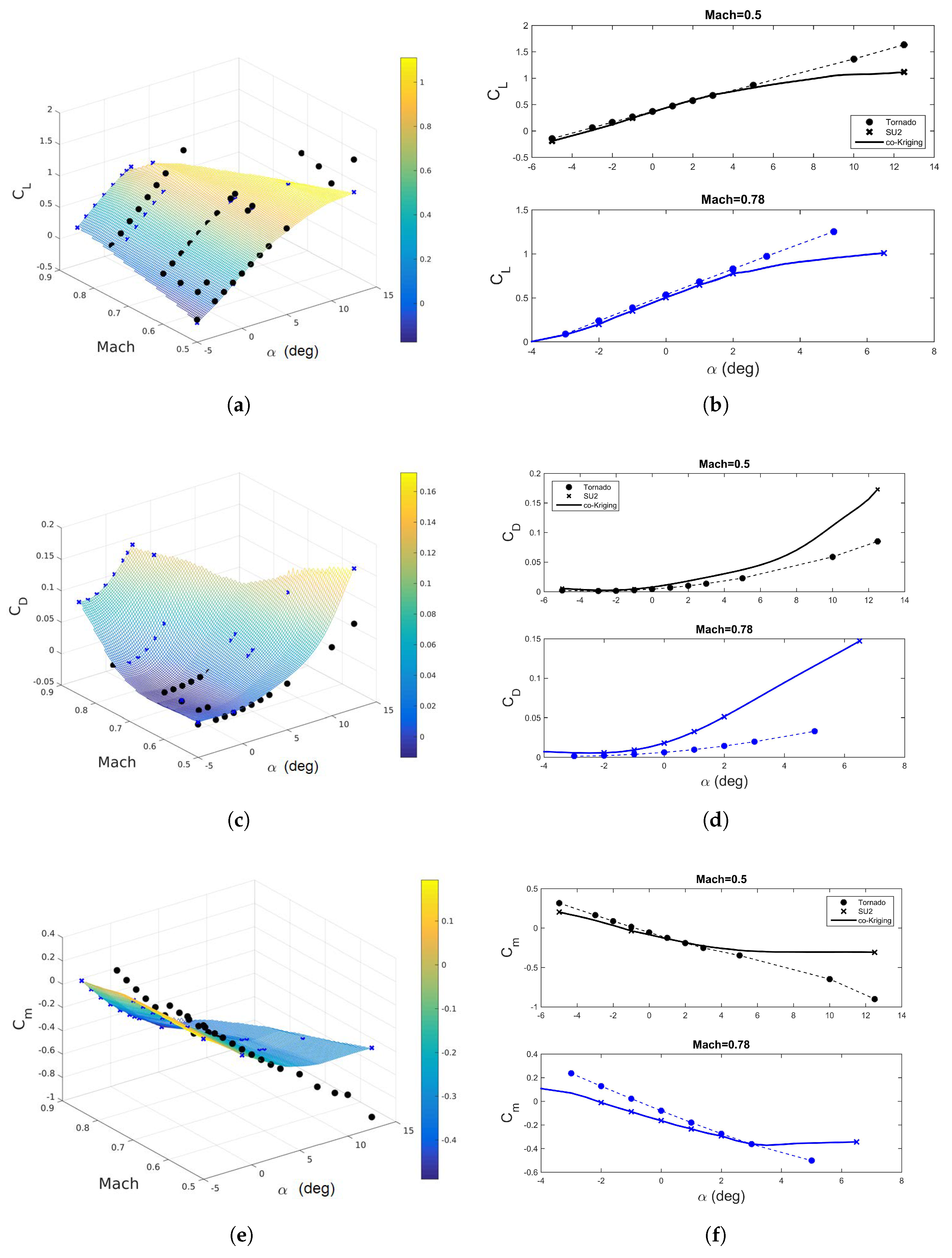
5.2. Multi-Fidelity Aerodynamics for Data Fusion
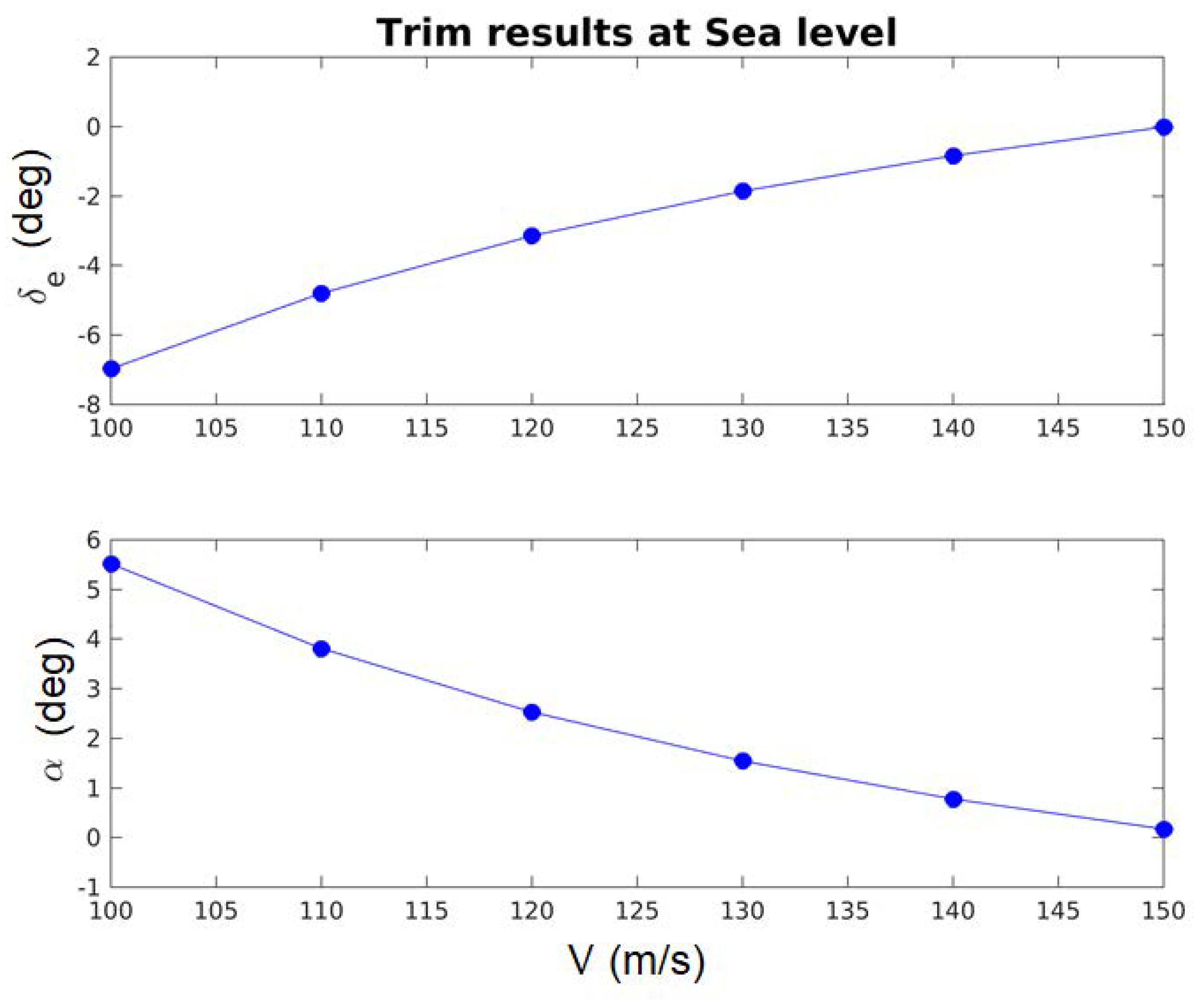
5.3. Aero-Data for Low Speed by the L1 Tool
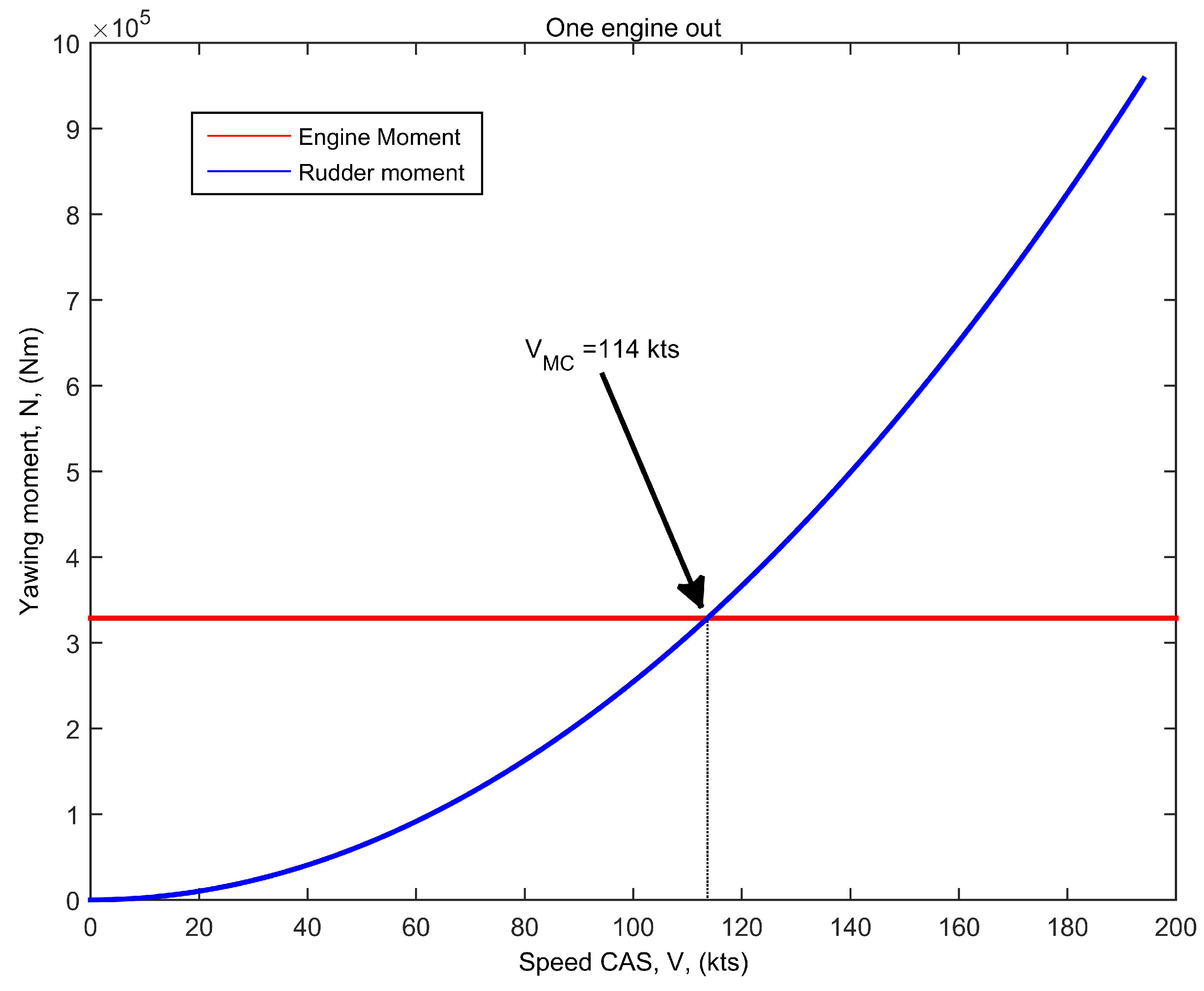
5.3.1. Sizing the Fin and Rudder for the One-Engine-Out Case
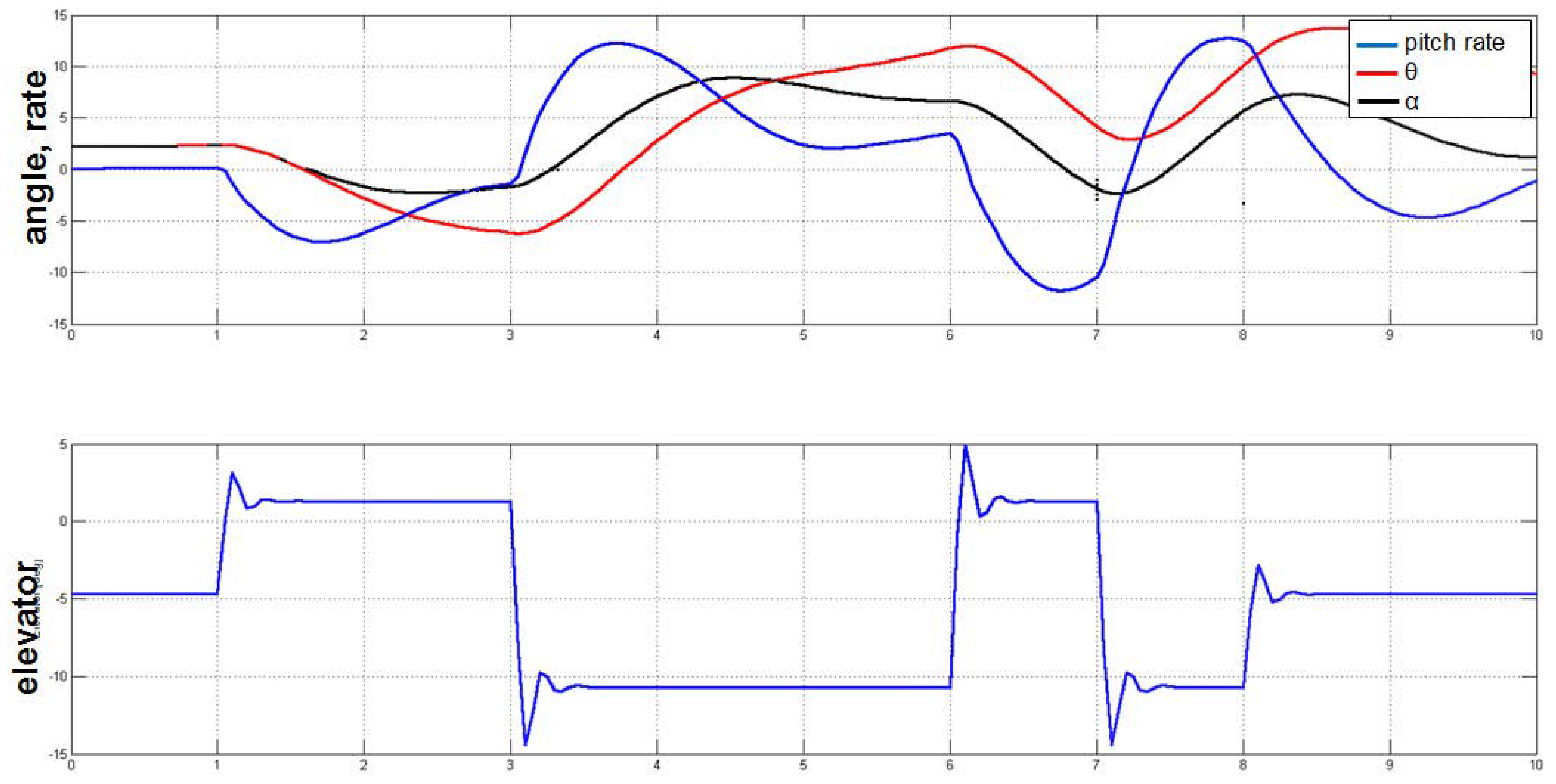
5.3.2. Handling Qualities
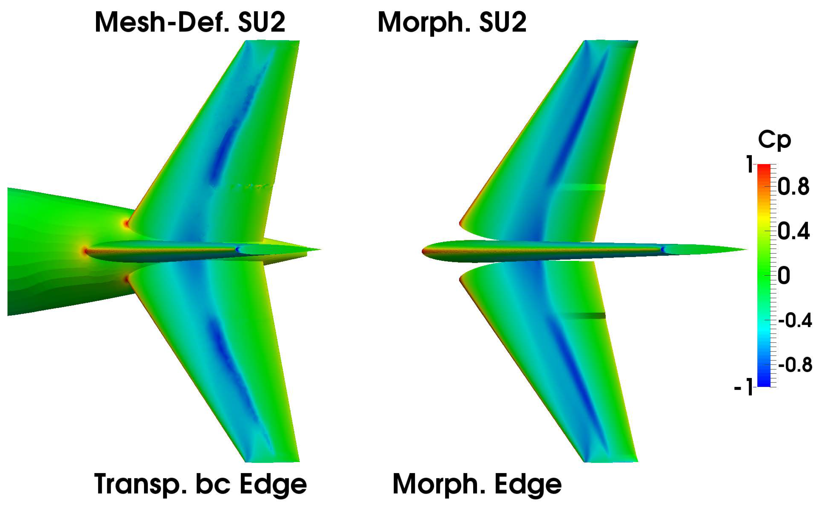
6. Euler Computation for Various Control Surface Models
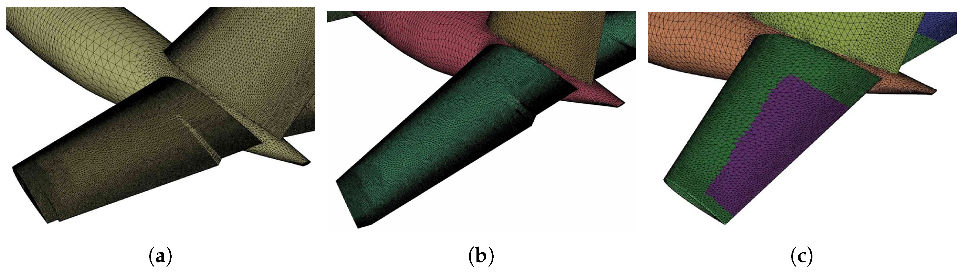
6.1. Modeling Movable Surfaces
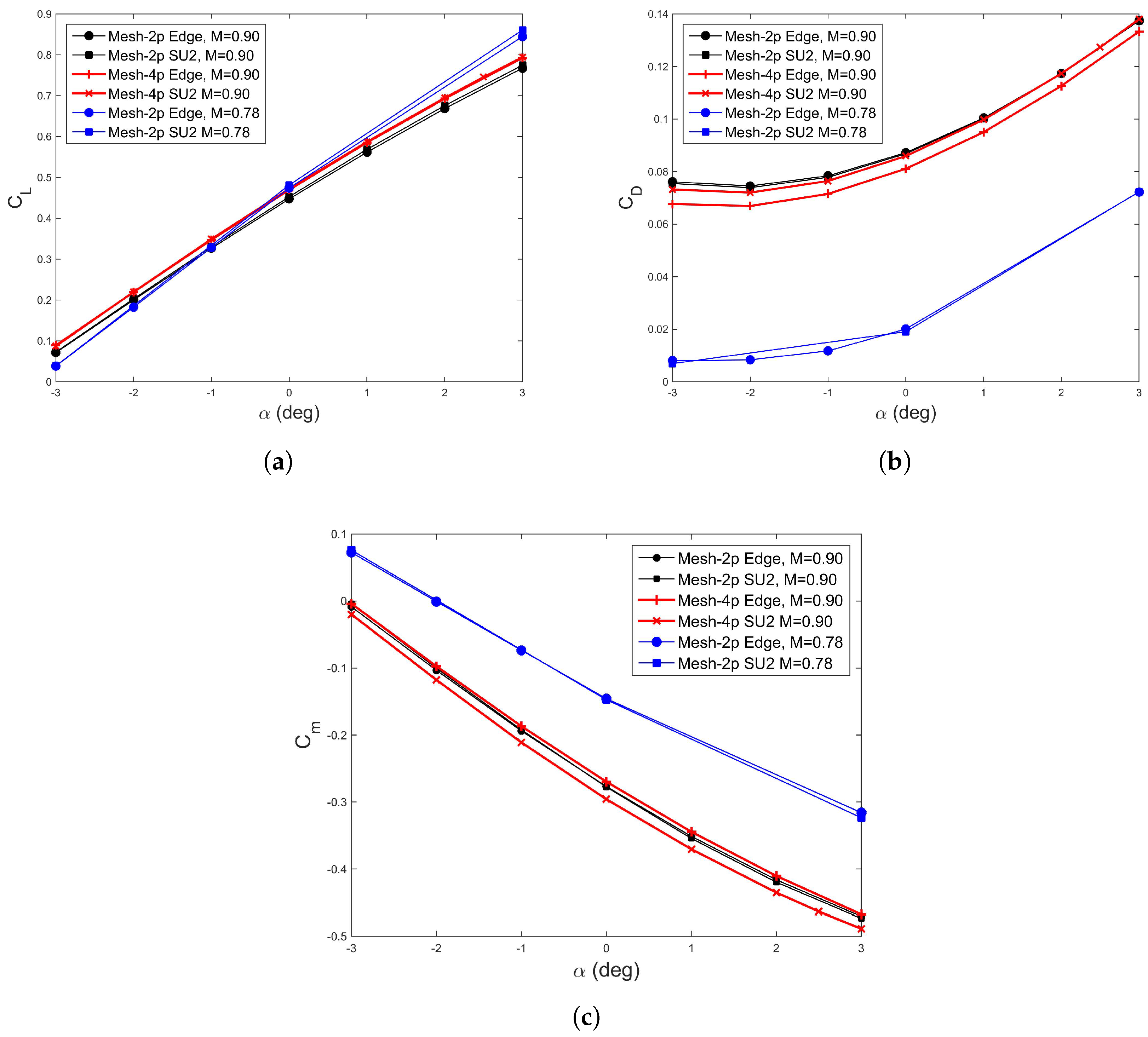
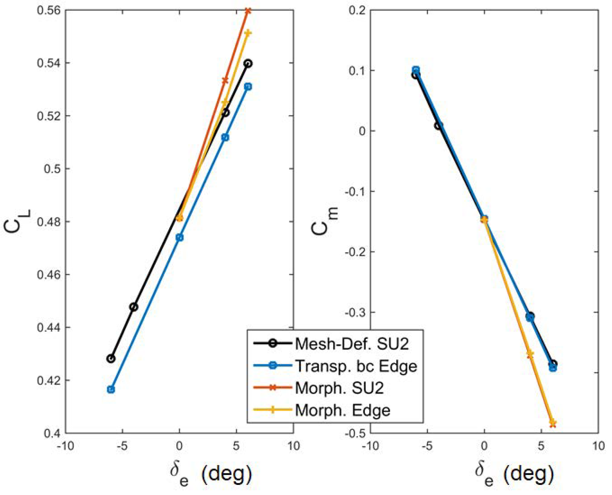
6.2. Results Comparison
- Mesh-Def(orm): Mesh deformation using FFD;
- Morph. (cs): Morphing the control surfaces by Sumo;
- Transp. b.c.: transpiration boundary conditions in Edge.
7. Conclusions
Author Contributions
Acknowledgments
Conflicts of Interest
Abbreviations
| AGILE | Aircraft 3rd Generation MDO for Innovative Collaboration of Heterogeneous Teams of Experts |
| API | Application Programming Interface |
| CAD | Computer Aided Design |
| CFD | Computational Fluid Dynamics |
| CPACS | The Common Parametric Aircraft Configuration Schema |
| CST | Class-Shape function Transformation |
| DES | Detached Eddy Simulation |
| FFD | Free-Form Deformation |
| GUI | Graphic User Interface |
| LES | Large-Eddy Simulation |
| MAC | Mean Aerodynamic Chord |
| MDA | Multidisciplinary Analysis |
| MDO | Multidisciplinary Design and Optimization |
| RANS | Reynolds-Averaged Navier–Stokes equations |
| TAS | True Air Speed |
| TE(D) | Trailing Edge (Device) |
| UI | User Interface |
| VLM | Vortex Lattice Method |
| XML | Extensible Markup Language |
| Symbols | |
| or AoA | Angle of Attack (deg) |
| Elevator deflection angle (deg) | |
| Attitude angle (deg) | |
| q | Pitch rate (deg/s) |
| Pressure Coefficient (-) | |
| Lift coefficient (-) | |
| Drag coefficient (-) | |
| Pitching moment coefficient (-) |
References
- Voskuijl, M.; de Klerk, J.; van Ginneken, D. Flight Mechanics Modelling of the Prandtl Plane for Conceptual and Preliminary Design; Springer: London, UK, 2012; Volume 66. [Google Scholar]
- Voskuijl, M.; La Rocca, G.; Dircken, F. Controllability of blended wing body aircraft. In Proceedings of the 26th Congress of International Council of the Aeronautical Sciences, Anchorage, AK, USA, 14–19 September 2008. [Google Scholar]
- Fengnian, T.; Voskuijl, M. Automated Generation of Multiphysics Simulation Models to Support Multidisciplinary Design Optimization. Adv. Eng. Inform. 2015, 29, 1110–1125. [Google Scholar]
- Foeken, M.J.; Voskuijl, M. Knowledge-Based Simulation Model Generation for Control Law Design Applied to a Quadrotor UAV. Math. Comput. Model. Dyn. Syst. 2010, 16, 241–256. [Google Scholar] [CrossRef]
- Raymer, D. Conceptual design modeling the RDS-professional aircraft design software. In Proceedings of the AIAA Aerospace Sciences Meeting, Orlando, FL, USA, 4–7 January 2011. [Google Scholar]
- Anemaat, W.A.; Kaushik, B. Geometry design assistant for airplane preliminary design. In Proceedings of the 49th AIAA Aerospace Sciences Meeting including the New Horizons Forum and Aerospace Exposition, Orlando, FL, USA, 4–7 January 2011. [Google Scholar]
- Gloudemans, J.R.; Davis, P.C.; Gelausen, P.A. A rapid geometry modeler for conceptual aircraft. In Proceedings of the 34th AIAA Aerospace Sciences Meeting and Exhibit, Reno, NV, USA, 15–18 January 1996. [Google Scholar]
- Tomac, M. Towards Automated CFD for Engineering Methods in Aircraft Design. Ph.D. Thesis, Royal Institute of Technology, KTH, Stockholm, Sweden, 2014. [Google Scholar]
- CPACS—A Common Language for Aircraft Design. Available online: http://www.cpacs.de/ (accessed on 7 February 2018).
- Böhnke, D.; Nagel, B.; Zhang, M.; Rizzi, A. Towards a collaborative and integrated set of open tools for aircraft design. In Proceedings of the 51st AIAA Aerospace Sciences Meeting including the New Horizons Forum and Aerospace Exposition, Grapevine, TX, USA, 7–10 January 2013; pp. 7–10. [Google Scholar]
- SUAVE—An Aerospace Vehicle Environment for Designing Future Aircraft. Available online: http://suave.stanford.edu/ (accessed on 20 March 2018).
- Lukaczyk, T.; Wendorff, A.; Botero, E.; MacDonald, T.; Momose, T.; Variyar, A.; Vegh, J.M.; Colonno, M.; Economon, T.; Alonso, J.J.; et al. SUAVE: An Open-Source Environment for Multi-Fidelity Conceptual Vehicle Design. In Proceedings of the 16th AIAA Multidisciplinary Analysis and Optimization Conference, Dallas, TX, USA, 22–26 June 2015. [Google Scholar]
- MacDonald, T.; Clarke, M.; Botero, E.M.; Vegh, J.M.; Alonso, J.J. SUAVE: An Open-Source Environment Enabling Multi-fidelity Vehicle Optimization. In Proceedings of the 18th AIAA Multidisciplinary Analysis and Optimization Conference, Denver, CO, USA, 5–9 June 2017. [Google Scholar]
- Zhang, M.; Bartoli, N.; Jungo, A.; Lammen, W.; Baalbergen, E. Data Fusion and Aerodynamic Surrogate Modeling for Handling Qualities Analysis. Prog. Aerosp. Sci. Spec. Issue 2018. submitted. [Google Scholar]
- AGILE EU Project Portal. Available online: http://www.agile-project.eu (accessed on 15 January 2018).
- Seider, D.; Fischer, P.; Litz, M.; Schreiber, A.; Gerndt, A. Open Source Software Framework for Applications in Aeronautics and Space. In Proceedings of the IEEE Aerospace Conference, Big Sky, MT, USA, 3–10 March 2012. [Google Scholar]
- Baalbergen, E.; Kos, J.; Louriou, C.; Campguilhem, C.; Barron, J. Streamlining cross-organisation product design in aeronautics. Proc. Inst. Mech. Eng. Part G J. Aerosp. Eng. 2016. [Google Scholar] [CrossRef]
- Moerland, E.; Ciampa, P.D.; Zur, S.; Baalbergen, E.; D’Ippolito, R.; Lombardi, R. Collaborative Architecture supporting the next generation of MDO within the AGILE Paradigm. Prog. Aerosp. Sci. Spec. Issue 2018. submitted. [Google Scholar]
- Van Gent, I.; Aigner, B.; Beijer, B.; Jepsen, J.; Rocca, G.L. Knowledge architecture supporting the next generation of MDO in the AGILE paradigm. Prog. Aerosp. Sci. Spec. Issue 2018. submitted. [Google Scholar]
- Jungo, A.; Vos, J.; Zhang, M.; Rizzi, A. Benchmarkig New CEASIOM with CPACS Adoption for Aerodynamic Analysis and Flight Simulation. Aircr. Eng. Aerosp. Technol. 2017, 90. [Google Scholar] [CrossRef]
- TIGL—Geometry Library to Process Aircraft Geometries in Pre-Design. Available online: https://github.com/DLR-SC/tigl (accessed on 30 November 2017).
- CPACS Documentation. Available online: https://github.com/DLR-LY/CPACS/tree/develop/documentation (accessed on 20 April 2018).
- Melin, T. Using Internet Interactions in Developing Vortex Lattice Software for Conceptual Design. Ph.D. Thesis, Department of Aeronautics, Royal Institute of Technology, KTH, Stockholm, Sweden, 2003. [Google Scholar]
- Tomac, M.; Eller, D. From Geometry to CFD Grids: An Automated Approach for Conceptual Design. Prog. Aerosp. Sci. 2011, 47, 589–596. [Google Scholar] [CrossRef]
- Si, H. TetGen: A Quality Tetrahedral Mesh Generator and 3D Delaunay Triangulator; Technical Report, User’s Manual; Technical Report No. 13; Numerical Mathematics and Scientific Computing, Weierstrass Institute for Applied Analysis and Stochastics (WIAS): Berlin, Germany, 2013. [Google Scholar]
- Anderson, J.D. Modern Compressible Flow with Historical Perspective, 3rd ed.; McGraw-Hill: New York, NY, USA, 2004. [Google Scholar]
- Katz, J.; Plotkin, A. Low-Speed Aerodynamics: From Wing Theory to Panel Methods; McGraw-Hill, Inc.: New York, NY, USA, 1991. [Google Scholar]
- Eliasson, P. Edge, a Navier-Stokes Solver for Unstructured Grids. In Finite Volumes for Complex Applications III; Elsevier: Amsterdam, The Netherlands, 2002; pp. 527–534. [Google Scholar]
- Palacios, F.; Colonno, M.R.; Aranake, A.C.; Campos, A.; Copeland, S.R.; Economon, T.D.; Lonkar, A.K.; Lukaczyk, T.W.; Taylor, T.W.R.; Alonso, J. Stanford University Unstructured (SU2): An open-source integrated computational environment for multi-Physics simulation and design. In Proceedings of the 51st AIAA Aerospace Sciences Meeting including the New Horizons Forum and Aerospace Exposition, Grapevine, TX, USA, 7–10 January 2013. AIAA 2013-0287. [Google Scholar]
- Economon, T.D.; Palacios, F.; Copeland, S.R.; Lukaczyk, T.W.; Alonso, J.J. SU2: An Open-Source Suite for Multiphysics Simulation and Design. AIAA J. 2015, 54, 828–846. [Google Scholar] [CrossRef]
- Palacios, F.; Economon, T.D.; Wendorff, A.D.; Alonso, J. Large-Scale Aircraft Design Using SU2. In Proceedings of the 53rd AIAA Aerospace Sciences Meeting, AIAA 2015-1946, Kissimmee, FL, USA, 5–9 January 2015. [Google Scholar]
- Griva, I.; Nash, S.G.; Sofer, A. Linear and Nonlinear Optimization, 2nd ed.; Society for Industrial Applied Mathematics: Philadelphia, PA, USA, 2009. [Google Scholar]
- Yousefi, K.; Razeghi, A. Determination of the Critical Reynolds Number for Flow over Symmetric NACA Airfoils. In Proceedings of the 2018 AIAA Aerospace Sciences Meeting, AIAA 2018–0818, Kissimmee, FL, USA, 8–12 January 2018. [Google Scholar]
- Forrester, A.; Keane, A. Engineering Design via Surrogate Modelling: A Practical Guide; John Wiley & Sons: Hoboken, NJ, USA, 2008. [Google Scholar]
- Federal Aircraft Administration. CFR 25.149; Technical Report, Retrieved 18 January 2018; Federal Aircraft Administration: Washington, DC, USA, 2018.
- Torenbeek, E. Synthesis of Subsonic Airplane Design; Delft University Press: Delft, The Netherlands, 1982. [Google Scholar]
- Etkin, B.; Reid, L.D. Dynamics of Flight: Stability and Control; John Wiley & Sons: Hoboken, NJ, USA, 1996. [Google Scholar]
- Pfeiffer, T.; Nagel, B.; Böhnke, D.; Voskuijl, M.; Rizzi, A. Implementation of a Heterogeneous, Variable-Fidelity Framework for Flight Mechanics Analysis in Preliminary Aircraft Design; Deutscher Luft-und Raumfahrtkongress: Bremen, Germany, 2011. [Google Scholar]
- Sederberg, T.W.; Parry, S.R. Free-Form Deformation of Solid Geometric Models. In Proceedings of the SIGGRAPH ’86 13th Annual Conference on Computer Graphics and Interactive Techniques, Atlanta, GA, USA, 1–5 August 1986; Volume 20, pp. 151–160. [Google Scholar]
- Zhang, M. Contributions to Variable Fidelity MDO Framework for Collaborative and Integrated Aircraft Design. Ph.D. Thesis, Royal Institute of Technology KTH, Stockholm, Sweden, 2015. [Google Scholar]
- Kulfan, B. Universal Parametric Geometry Representation Method. J. Aircr. 2008, 45, 142–158. [Google Scholar] [CrossRef]


| Model Type | Solver | (deg) | (deg) |
|---|---|---|---|
| Mesh-deform | SU2 | 0.0092 | −0.0399 |
| Morph. cs | SU2 | 0.0130 | −0.0565 |
| Morph. cs | Edge | 0.0117 | −0.0557 |
| Transp. b.c. | Edge | 0.0095 | −0.0411 |
© 2018 by the authors. Licensee MDPI, Basel, Switzerland. This article is an open access article distributed under the terms and conditions of the Creative Commons Attribution (CC BY) license (http://creativecommons.org/licenses/by/4.0/).
Share and Cite
Zhang, M.; Jungo, A.; Gastaldi, A.A.; Melin, T. Aircraft Geometry and Meshing with Common Language Schema CPACS for Variable-Fidelity MDO Applications. Aerospace 2018, 5, 47. https://doi.org/10.3390/aerospace5020047
Zhang M, Jungo A, Gastaldi AA, Melin T. Aircraft Geometry and Meshing with Common Language Schema CPACS for Variable-Fidelity MDO Applications. Aerospace. 2018; 5(2):47. https://doi.org/10.3390/aerospace5020047
Chicago/Turabian StyleZhang, Mengmeng, Aidan Jungo, Alessandro Augusto Gastaldi, and Tomas Melin. 2018. "Aircraft Geometry and Meshing with Common Language Schema CPACS for Variable-Fidelity MDO Applications" Aerospace 5, no. 2: 47. https://doi.org/10.3390/aerospace5020047
APA StyleZhang, M., Jungo, A., Gastaldi, A. A., & Melin, T. (2018). Aircraft Geometry and Meshing with Common Language Schema CPACS for Variable-Fidelity MDO Applications. Aerospace, 5(2), 47. https://doi.org/10.3390/aerospace5020047