Project Report

Aircraft Geometry and Meshing with Common Language Schema CPACS for Variable-Fidelity MDO Applications

1
Airinnova AB, 18248 Stockholm, Sweden
2
CFS Engineering, 1015 Lausanne, Switzerland
*
Author to whom correspondence should be addressed.
Aerospace 2018, 5(2), 47; https://doi.org/10.3390/aerospace5020047
Submission received: 1 March 2018 / Revised: 16 April 2018 / Accepted: 19 April 2018 / Published: 24 April 2018
(This article belongs to the Special Issue Computational Aerodynamic Modeling of Aerospace Vehicles)

Abstract

:
This paper discusses multi-fidelity aircraft geometry modeling and meshing with the common language schema CPACS. The CPACS interfaces are described, and examples of variable fidelity aerodynamic analysis results applied to the reference aircraft are presented. Finally, we discuss three control surface deflection models for Euler computation.

1. Introduction

The design of aircraft is inherently a multi-disciplinary undertaking, during which data and information must be exchanged between multiple teams of engineers, each with expertise in a specific field. Managing the transmission, possibly translation and storage of data between collaborating groups is complex and error-prone. The adoption of a standardized, data-centric scheme for storage of all data improves consistency and reduces the risk of misconceptions and conflicts. In order to achieve this effectively, an initial effort must be made to develop suitable interfaces between the analysis modules and the data archive.
Furthermore, each phase of the design process poses different requirements on the fidelity and resolution of the design and analysis tools. For stability and control analysis, as well as for flight simulation, look-up tables for aerodynamic forces, moments and derivatives need to be generated. Different flight analysis tools require different tables/input formats. For example, the flight analyzer and simulator PHALANX [1,2,3,4] developed by Delft University of Technology requires a set of three-dimensional tables of force and moment coefficients with the effect of each control channel acting individually. Multi-fidelity aerodynamic modeling aims to cover the flight state parameter space of the entire flight envelope with an optimal distribution of computational resources. This again requires a standardized, data-centric scheme to host the data, which can be used for variable fidelities.
The label Li , where i = 0 , 1 , 2 , 3 , is used to classify the fidelity level of a computational model and its software implementation:
L0:
handbook methods, based on statistics and/or empirical design rules;
L1:
based on simplified physics, can model and capture a limited amount of effects. For example, the linearized-equation models, the Vortex-Lattice Method (VLM) or the panel method in aerodynamics;
L2:
based on accurate physics representations. For example, the non-linear analysis, Euler-based CFD;
L3:
represents the highest end simulations, usually used to capture detailed local effects, but do not allow wide exploration of the design space due to computational cost. Additionally, the modeling may require extensive ad hoc manual intervention. For example, the highest fidelity methods, RANS-based CFD.
To construct a reasonable variable fidelity CFD analysis system, one should consider the variable fidelity of the geometrical representations corresponding to the CFD tools. The level of detail in the geometry gathered from a CAD system needs to match the CFD model fidelity. The chosen high fidelity model must be as accurate as possible and can reflect all considered complex flow characteristic; the chosen low-fidelity model must reflect the basic flow characteristics and be as effective as possible. In the conceptual design stage, the usual practice, for example, in the RDS [5], the AAA [6] and the VSP [7] software systems, is to use a purpose-specific CAD that is simpler than the commercial systems, and fewer parameters need to be used for the configuration layout at this stage in the design cycle [8]. However, for some innovative configurations, different ranges of flight conditions or more detailed analyses, the simplified CAD is not sufficient for a higher fidelity CFD analysis; thus, an enriched geometry definition with more parameters is needed. The Common Parametric Aircraft Configuration Schema (CPACS) [9,10], defining the aircraft configuration parametric information in a hierarchical way, gives the opportunity to incorporate different fidelity CFD tools with one single CPACS file. For different fidelity tools to be used, the corresponding geometry information can be imported/retrieved from the common CPACS file to match the model fidelity.
SUAVE, Standford University Aerospace Vehicle Environment [11,12,13], which is also a multi-fidelity design framework developed at Stanford University, stores the aircraft geometry information using an inherent defined data class, which can be easily modified. The aerodynamic solutions can be generated from simple models within SUAVE or easily imported from external sources like CFD or wind tunnel results. The aircraft analysis in SUAVE is calculated with a so-called “fidelity zero” VLM to predict lift and drag, with a number of corrections such as the compressibility drag correction, parasite drag correction, etc. [12], to adapt the VLM prediction to a wider range (transonic and supersonic flow regions). It incorporates the “multi-fidelity” aerodynamics through the provided response surface by combining the different fidelity data. However, currently, SUAVE is still working on connecting higher fidelity models directly to it; the response surfaces are only available to incorporate higher fidelity lift and drag data from the external sources [12]. At this point, one cannot guarantee that the geometry information used for different fidelity tools is consistent during data exchanging, transferring and translating. Moreover, the prediction is only limited to lift and drag, so that it might not be easy for engineers to look into the physical details for a better design, for example, the pressure isobars and distributions, the laminar flows, transitions and the shock forming, etc. Thus, a dataset that can store complete and consistent information for different fidelity tools to solve the physical flows is desired. The CPACS-based multi-fidelity aerodynamic tools show a great consistency due to the one data-centric schema, and the automation of the progressive process can thus be implemented and realized with minimum data loss.
With all the computed aerodynamic data at hand, an important task is to construct surrogate models that integrate all analysis results computed by tools of different fidelity. Such data fusion applications are enabled by standardization of the data—format, syntax and semantics—of the aerodynamic simulation tools. The work in [14] describes the workflow of an automatic data fusion process for CPACS [9,10]. The application was developed in the EU research project Aircraft 3rd Generation MDO for Innovative Collaboration of Heterogeneous Teams of Experts (AGILE) [15], where every module (the aerodynamic module, the sampling module, the surrogate modeling module) communicates by CPACS files.
This paper will address other aspects of the work in [14], namely how the different fidelity tools in the aerodynamic module communicate and how a look-up table of the aero-dataset can be obtained automatically from the tools (L1 and L2 in this paper). Section 2 describes the CPACS file definition in more detail, especially the geometry definitions, which are important for CFD mesh generators. Section 3 details the CPACS interfaces for variable fidelity analysis. Section 4 gives an overview of the CFD flow solvers used in the work. Section 5 presents the applications to the test case using variable fidelity tools. Section 6 discusses different modeling approaches for control surfaces used for Euler simulations, and finally, Section 7 summarizes the conclusions of the work.

1.1. Background

AGILE is an EU-funded Horizon 2020 project coordinated by the Institute of Air Transportation Systems of the German Aerospace Center (DLR). Its objective is to implement a third generation multidisciplinary optimization process through efficient collaboration by international multi-site design teams. The 19 partners bring different knowledge and competences regarding aircraft design and optimization. As mentioned above, such a collaboration is enabled by the adoption of a common data storage format. To this end, AGILE relies on the XML format CPACS (Common Parametric Aircraft Configuration Schema) [9,10] in development at DLR since 2005.
The RCE (Remote Component Environment) integration environment and workflow manager [16] controls and executes the sequence of analysis modules and manages the data transport and translation, as well as logging the process. RCE makes it easy to set up an MDO workflow also with modules running on remote hosts. That is handled by the BRICS (Building blocks for mastering network Restrictions involved in Inter-organisational Collaborative engineering Solutions) [17] system, which supports remote execution and data transport. The request can be with “engineer in the loop” for a remote expert to run the calculation or for an automated workflow to be run without user intervention. The input is generally a CPACS file containing all the information required. The new data generated are added to the CPACS file and sent back to the requester. More details about the AGILE collaborative approach can be found in [18,19].
The variable fidelity aerodynamic tools read a CPACS file, analyze the corresponding information extracted from the file, run the calculation and store the new data (e.g., aero-data tables) back to the CPACS file. CPACS supports a very flexible user-defined node feature (cpacs.toolspecific) to handle parameters for the computational models, which are relevant only for a specific tool [20].

1.2. Aerodynamic Model Description

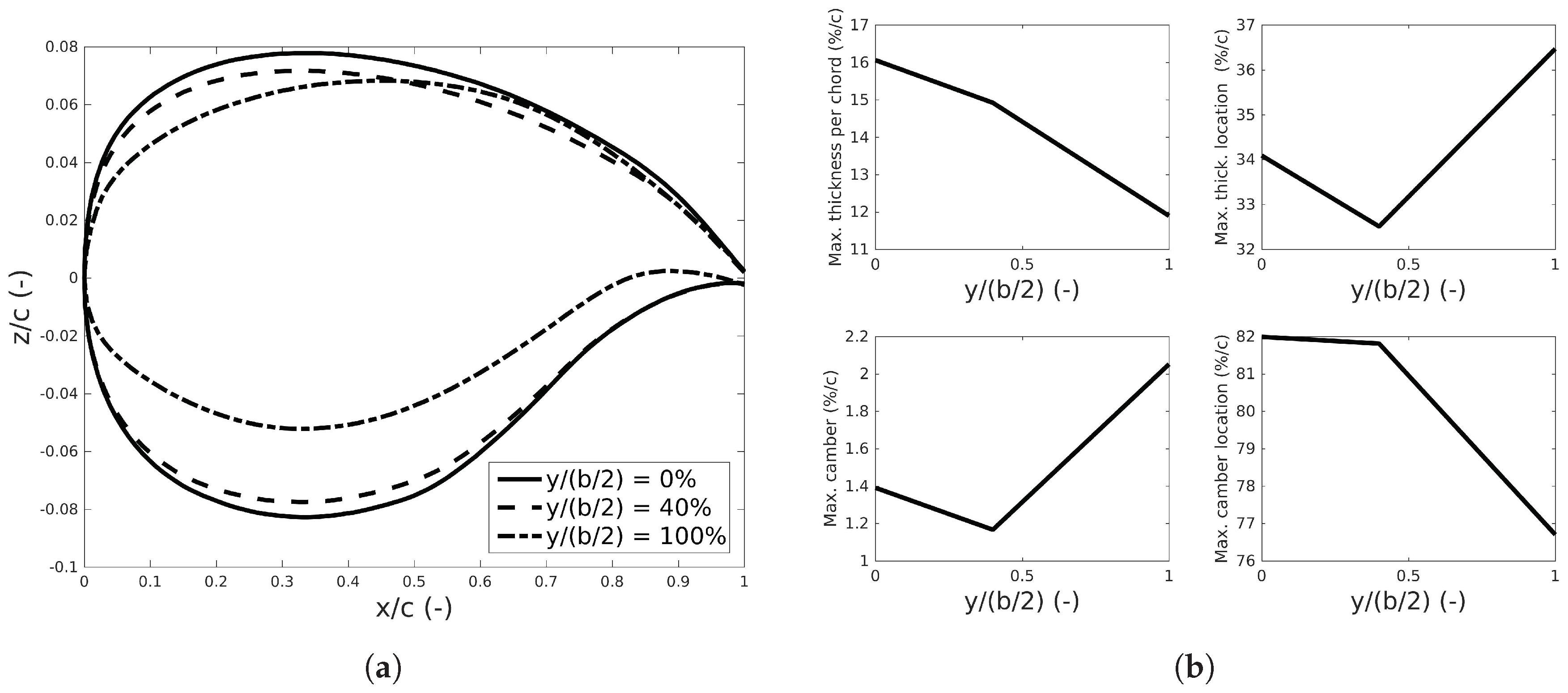
The test case is the reference aircraft used in AGILE, a regional jet-liner, which was analyzed and simulated using the AGILE MDO system, without experimental data. This virtual aircraft is similar to an Airbus 320 or a Boeing 737. The reference aircraft is defined in CPACS [9] format, shown in Figure 1. Its aspect ratio is 9.5, and the detailed information of the airfoils along the aircraft span is shown in Figure 2. Figure 2a shows the plots of the airfoil along the three stations of the semi-span ( b / 2 ), with the root at 0%, the kink at 40% and the tip at 100%. Figure 2b shows the maximum thickness and cambers per chord along the semi-span, as well as the corresponding locations of the local chords. It should be noted that the design exercises are carried out as if in an early design stage, so for instance, no engine is modeled. The configuration was also used in previous studies, to benchmark the conceptual design software CEASIOM [20] and to validate the AGILE data fusion tool [14] for building multi-fidelity aero-datasets. Some of the results shown in this paper are consistent with the previous simulations in [14,20], that the configuration is unchanged and the same CPACS file for geometry definition is used to assure a consistent and continuous investigation of the tools and methods.

2. CPACS File Description

2.1. The CPACS Hierarchical Data Definition Structure

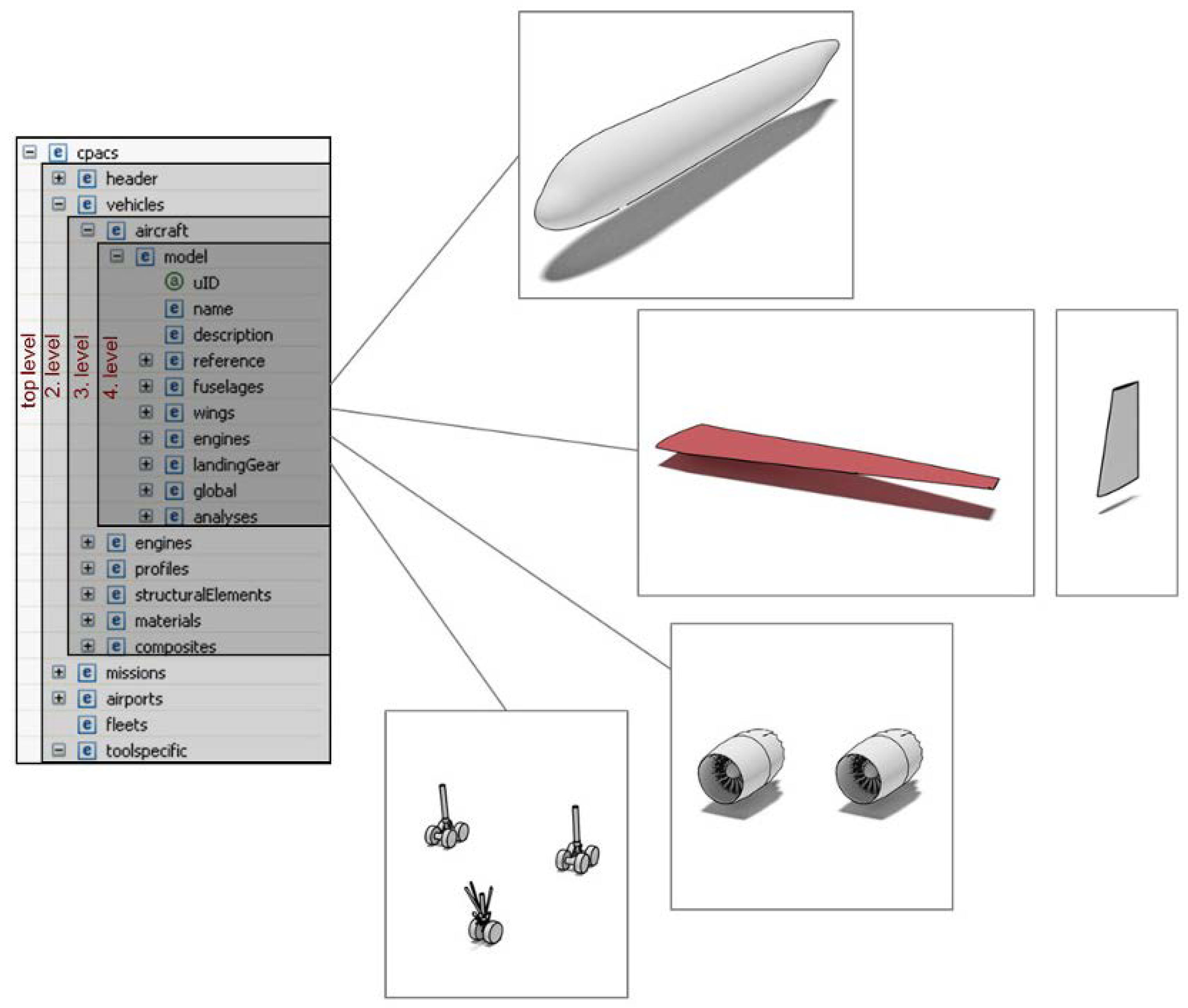
Thanks to its hierarchical structure, CPACS is capable of hosting the entire aircraft geometry, as well as additional design information relating to flight missions, airports, propulsion systems and aerodynamic datasets; see Figure 3.
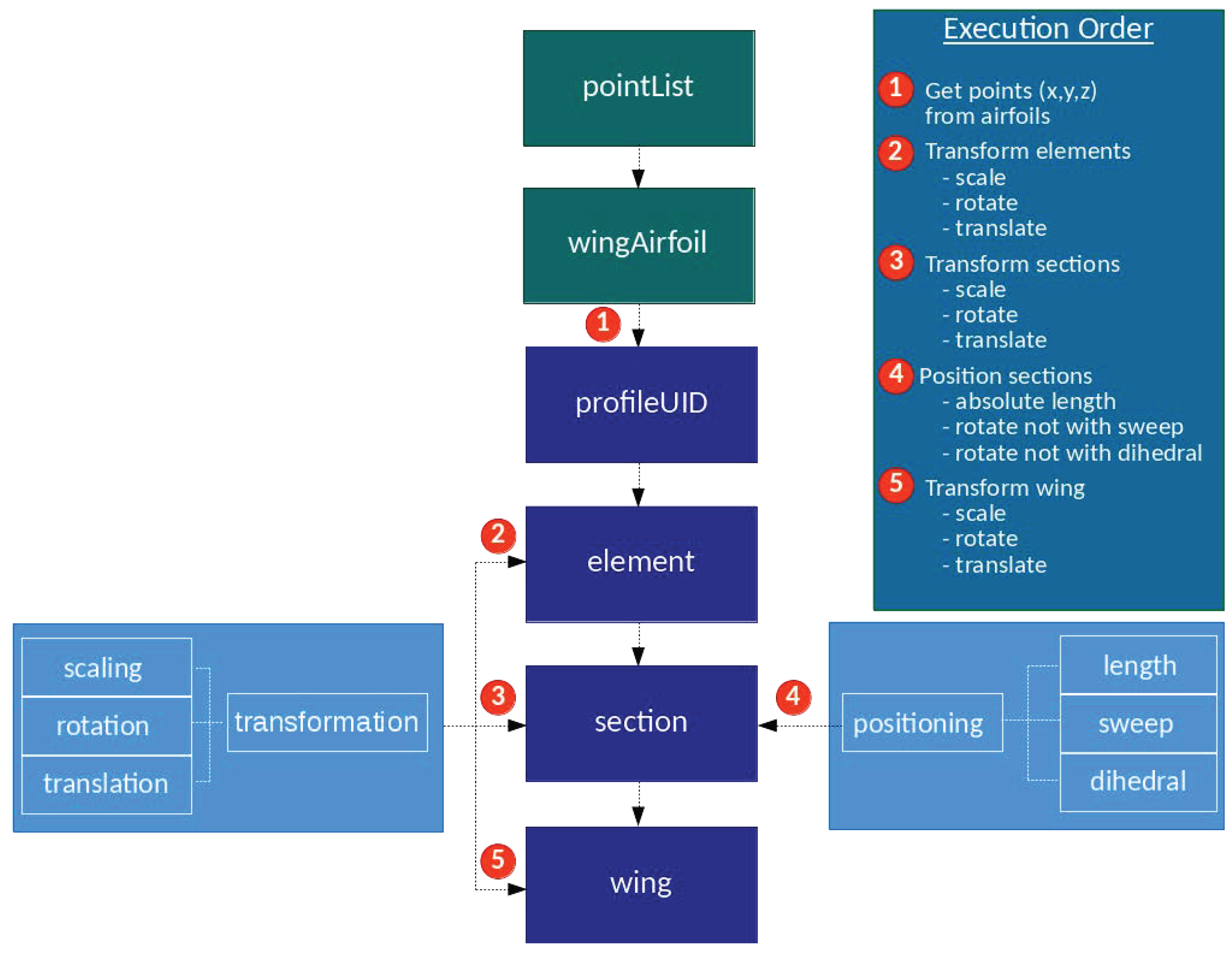
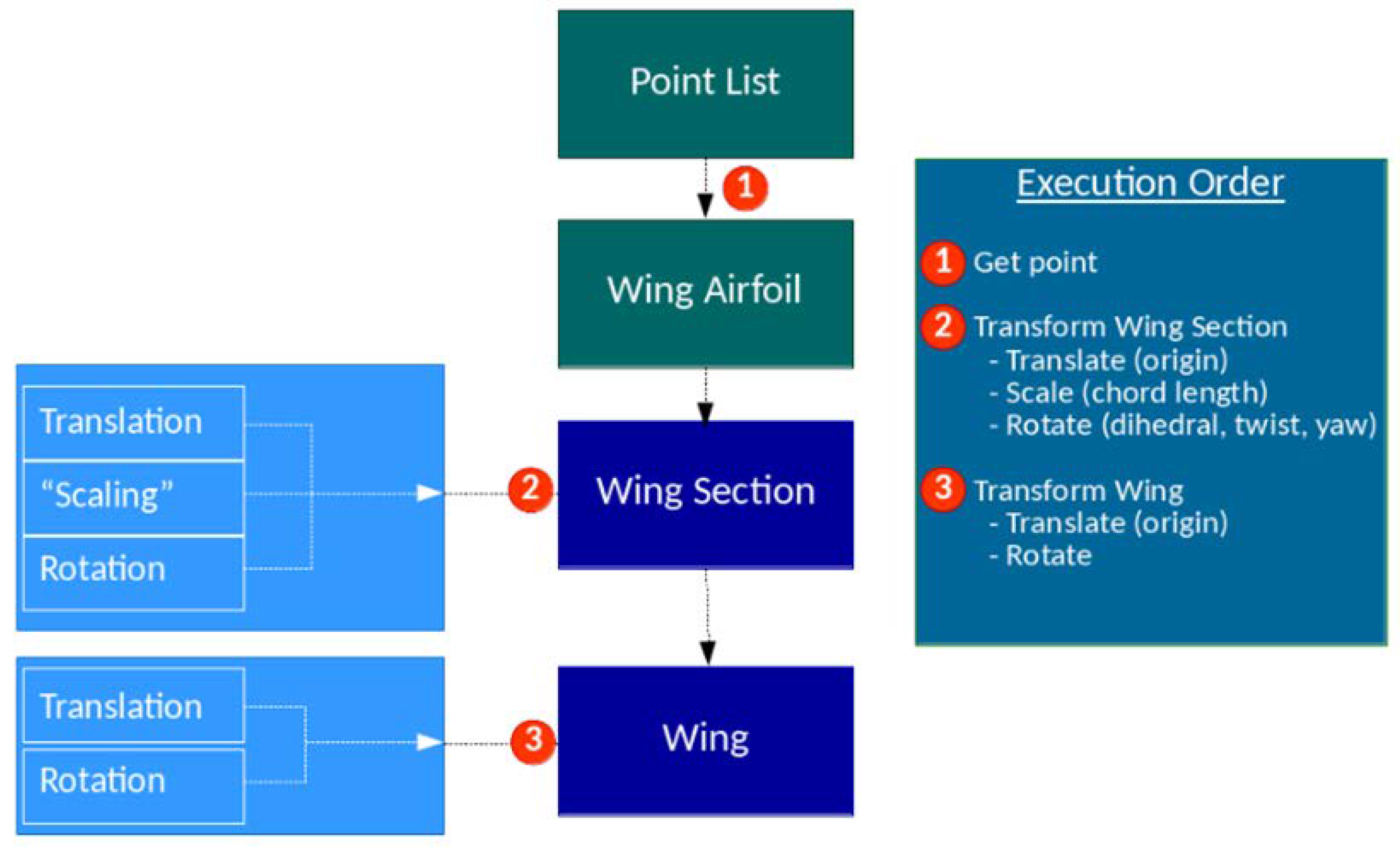
The hierarchical data structure is used to define the order of “construction” of each aircraft component (fuselage, wing, etc.). Figure 4 shows, for example, the construction of a wing geometry from the CPACS data. Other parts of the aircraft are treated similarly. For wings, the construction begins with ordered lists of points, which define airfoils. A library of airfoils identified by profileUIDs can be stored in the CPACS geometry definition and from these, a list of wing elements. An element is defined by its profileUID and a transformation: the scaling along coordinate directions, a 3D rotation and a translation. Two such elements define a section, the positioning of which is effected by a length, sweep angle and a dihedral angle. The sections are assembled to form a wing, to which it is possible once more to apply a transformation. Symmetries can be used to create instances of wings already defined, A single CPACS file holds a set of named lifting surfaces defined in this way. It must be noted that a given wing geometry allows multiple distinct CPACS definitions.

2.2. The CPACS Control Surface Definition

On each wing, several types of control surfaces may be defined: leading edge devices, spoilers and Trailing Edge Devices (TEDs). A detailed explanation of their definition is given here only for TEDs. It is analogous for the other devices. In order to define a TED, a componentSegment first needs to be created. Each componentSegment is defined from two, not necessarily contiguous, wing elements. Each wing must have at least one componentSegment to define the wing structure, fuel tanks, control surfaces, etc. Each corner of the outer shape of the control surface is defined by its relative position in the span- and chord-wise directions of the componentSegment, as shown in Figure 5, requiring eight values to be specified. For TEDs, corner points that are not explicitly defined lie on the trailing edge of the wing. In addition to these points, the hingeLine must also be defined, by the relative position of its inner and outer points in the span- and chord-wise directions, as well as their “vertical” position from 0 = lower wing surface to 1 = upper wing surface.
A control surface movement, called a step, is defined by an angle of rotation around the hinge line and a translation of the rotated surface, to allow the definition of flap movements. A deployment is then defined by interpolation in the table of steps.
The deflected control surfaces are modeled without gaps in this work. Thus, the coordinates of a control surface quadrilateral (see a TED example in Figure 5) are imported from the outerShape node affiliated with each defined control surface. The information is then interpreted by the different models in the CFD tools.

3. Geometry and CPACS Interfaces for Variable Fidelity Tools

Our focus is on multi-fidelity aerodynamic analysis, as a sub-task of MDO. The CPACS database acts as a single source of information in our multi-site collaborative environment.
Aircraft geometry modeling and mesh generation tools for L1 and L2, respectively, Tornado [23] and Sumo/TetGen [24,25], will be discussed next. Tornado is a VLM implementation for assessing aero-forces and moments on rigid lifting surfaces. Sumo/TetGen is an automatic volume mesh generator for CFD. It is fully automatic for the generation of isotropic tetrahedral grids for Euler solvers. Its Pentagrow [8] module provides semi-automatic mesh generation for RANS.

3.1. CPACS-Tornado Interface

Tornado [23], originally written in MATLAB, computes the aerodynamic coefficients and their first order derivatives for lifting surfaces at low speeds. The lifting surfaces are modeled as cambered lamina. The horseshoe vortices can be defined with seven segments to model the geometry of trailing edge movable surfaces. Leading edge movable surfaces can be similarly modeled, but seldom are, since such devices are for high-lift, high-alpha, augmentation, which VLM cannot reliably predict. The steady wake can be chosen fixed relative to the wing or to follow the free stream. Effects of compressibility at high Mach numbers (<0.75) are included through the Prandtl–Glauert correction [26]. The induced drag can be calculated by the Kutta–Joukowski law (default) or Trefftz-plane integration [27]. In the latest version, some additional features are included:
  • Aircraft configuration visualization including fuselage representation and control surface identifications;
  • Fast MEX-compiled version of core-functions for matrix computations;
  • All-moving surfaces and overlapped movable surfaces.
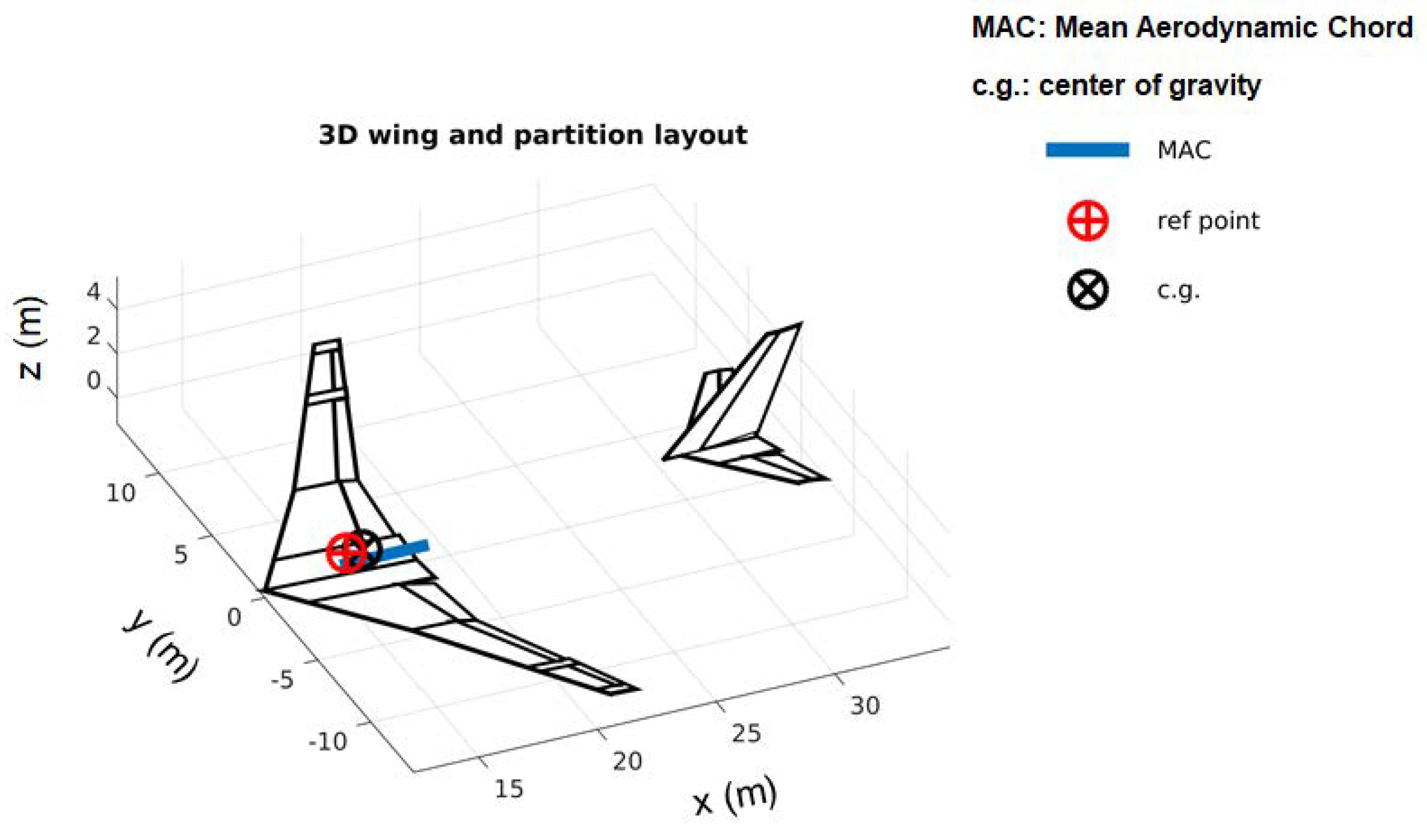
Tornado can import/export CPACS files via a separate wrapper also written in MATLAB. The wrapper reads the geometric information, as well as the paneling and flight conditions from CPACS, translates them into the Tornado native data structures and writes the computed results back to CPACS. Figure 6 shows the visualization of the configuration and panel distributions for the reference aircraft.

PyTornado: A VLM Solver with Native CPACS Compatibility

The Tornado internal geometry definition differs from the hierarchical geometry definition of CPACS. This is the leading motivation for the development of a VLM solver with native CPACS compatibility. The outcome is the PyTornado implementation written in Python and C++.
It inherits the essential analysis capabilities of the mature MATLAB Tornado code. Nonetheless, it can be considered as an independent program for VLM aerodynamics, with its own definition of input and output systems.
PyTornado is structured as two parts:
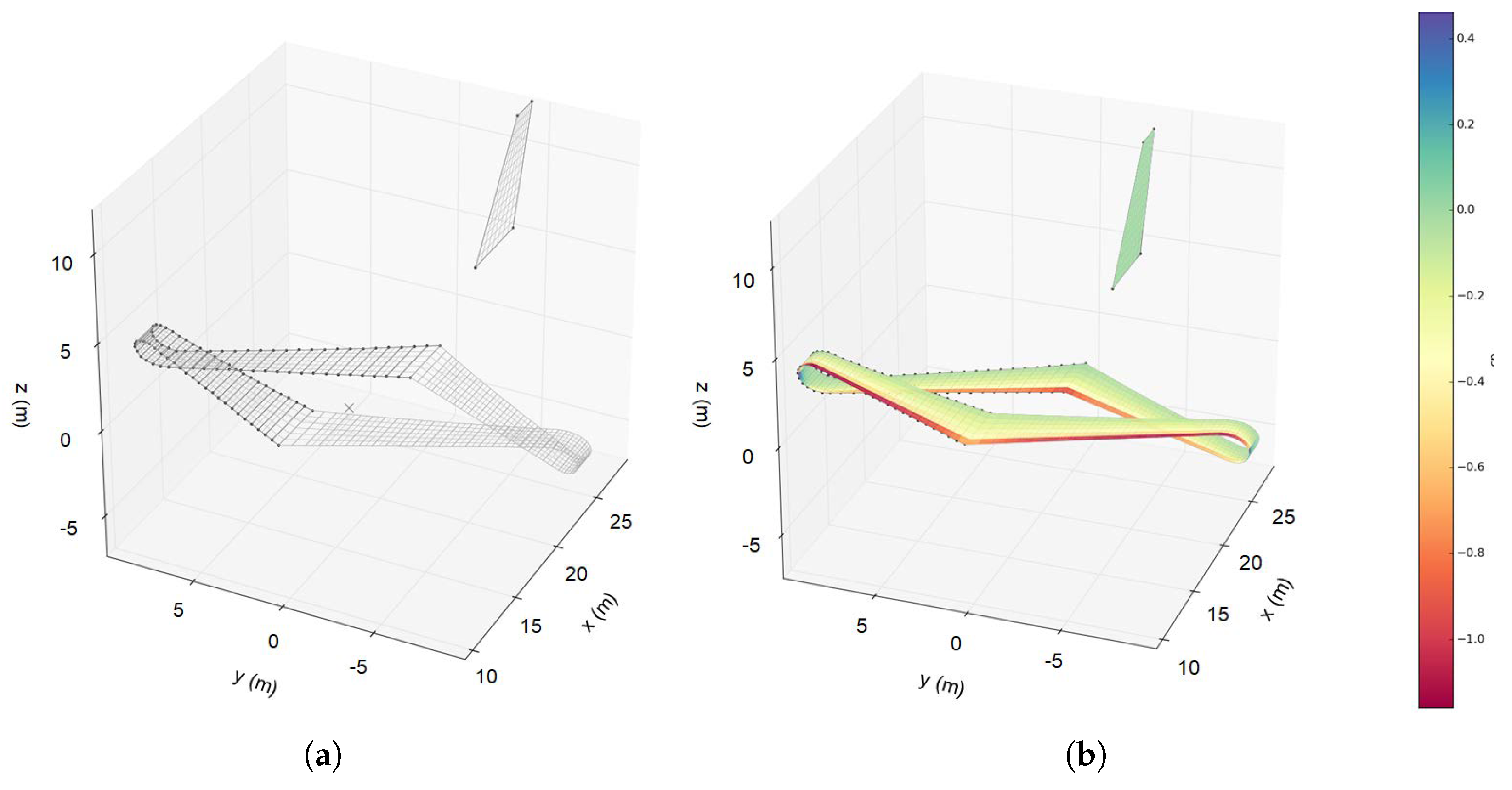
  • A Python wrapper, dedicated to high-level tasks such as communication with CPACS, pre- and post-processing for VLM, as well as visualization of the model and generated results; see Figure 7a,b,
  • The actual VLM solver, re-structured and re-written in C++ from the MATLAB Tornado VLM solver with performance in mind.
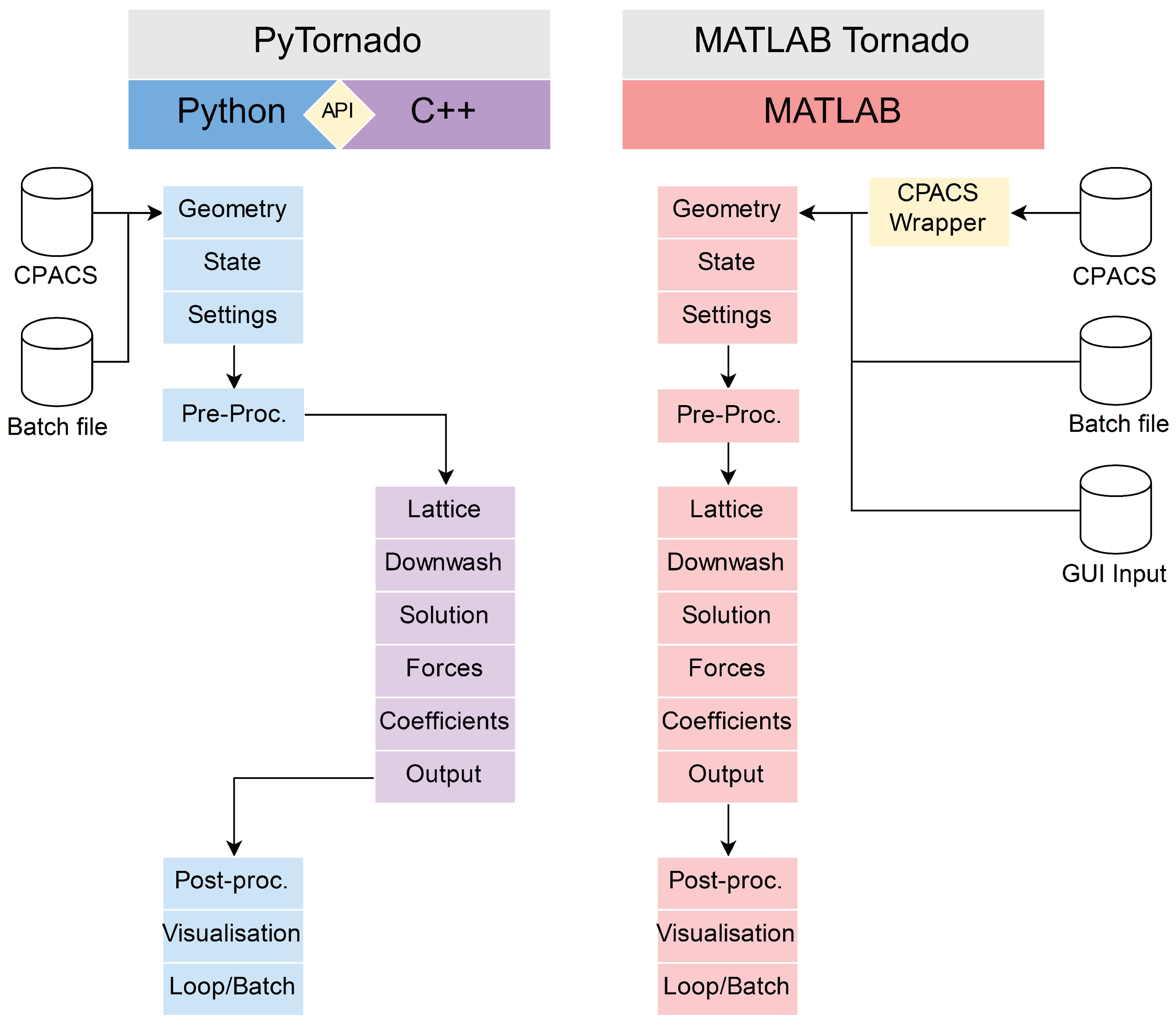
The user or an external program can use PyTornado as a computational service through the wrapper, which controls the execution steps.
PyTornado is a lightweight, fast and flexible VLM code. Its native compatibility with CPACS and the choice of Python as a main programming language make it a promising candidate for effective integration in larger analysis and optimization frameworks. Future development will be aimed at extending the Python wrapper functionality and completing the C++ solver with further analysis features. The core functions of the solver are exposed to the wrapper through the built-in C++ API of Python and NumPy ( The fundamental package for scientific computing with Python, http://www.numpy.org/). Thus, data transfer between the components occurs effectively in-memory. This design leverages the performance of C++ where required and the flexibility of Python for its high-level features and interface. Seamless integration of PyTornado with CPACS is enabled by its internal geometry definition, which closely corresponds to the hierarchical structure of the file format. Thus, operations on engineering/design parameters in CPACS can be translated to geometric data for VLM analysis without additional user effort.
Figure 8 shows the computational workflows. PyTornado, in its present state of completeness, is already an improvement over the MATLAB implementation both in performance and flexibility. The seamless integration of CPACS is a significant merit, leaving it open for extension and coupling with other tools, e.g., for structural analysis. PyTornado is currently still under development for further validations, with more features to be imported from CPACS files.

3.2. CPACS-Sumo Interface

The Euler (L2) and RANS (L3) flow models need a computational mesh adapted to the solver fidelity. This section introduces the mesh generation tool Sumo for L2 analysis and its interface with CPACS. Sumo can also generate RANS (L3) meshes with Pentagrow [8]; note that the RANS simulations are only used for validation in this paper (see Section 5.1).

3.2.1. Sumo: A Gateway from CPACS to Higher-Fidelity Aerodynamics

Sumo [24] is a graphic tool for rapid modeling of aircraft geometries and automatic unstructured surface mesh generation. It is not a full-fledged CAD system, but rather an easy-to-use sketchpad, highly specialized towards aircraft configurations in order to streamline the workflow. Isotropic tetrahedral volume meshes for Euler computation can be generated from the surface mesh, by the tetrahedral mesh generator TetGen [25].
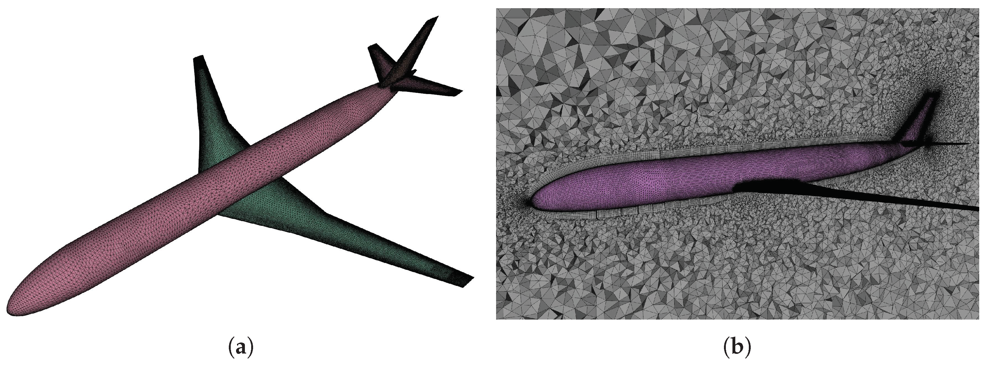
Pentahedral boundary layer elements for RANS solvers can also be (semi-)automatically generated by the Pentagrow [8] module in Sumo after the surface mesh is generated, before creation of the volume mesh by TetGen. Pentagrow sets up the prismatic element layers on the configuration surface from a configuration file with a list of user-defined parameters such as the first cell height, the total number of layers, the growth rate, etc. The volume mesh can be exported in various formats including CGNS (the CFD General Notation System), TetGen’s plain ASCII format and native formats for the CFD solvers Edge [28] and SU2 [29,30,31]. Mesh examples are shown in Figure 9a,b.

3.2.2. The Interface CPACS2SUMO

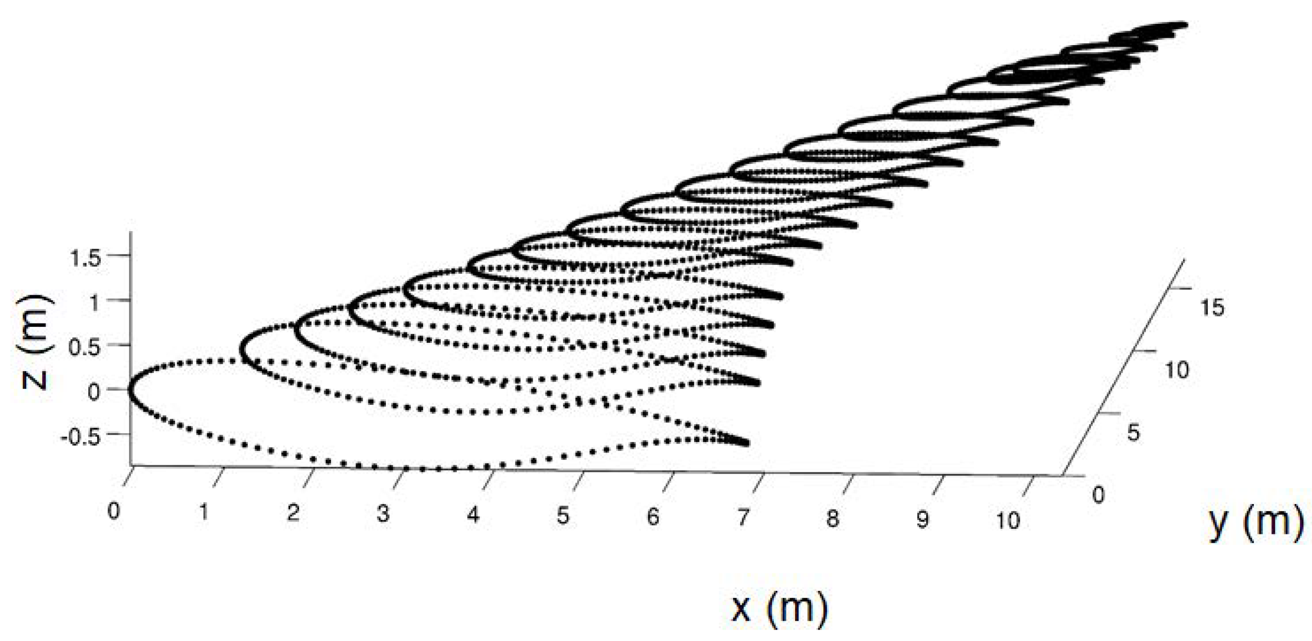
The aircraft configuration defined in a CPACS XML file is converted into a Sumo [24] native .smx file by the CPACS2SUMO Python converter without manual intervention. This conversion is relatively straightforward since both formats define aircraft in a similar way. Fuselage and wings are created from a gathering of sections placed in a certain order. Each section is defined by a 2D profile written as a list of points. Then, these profiles can be scaled, rotated and translated to form the desired shape. Figure 10 shows how Sumo represents a wing as a stack of airfoils. The 3D wing surface is lofted from the sections by Bézier or B-spline surfaces.
The CPACS format allows quite a general definition of cross-sections. For instance, a CPACS cross-section may be placed in the global coordinate system via reference to any other section (see Figure 4), whereas Sumo uses the order of the sections as they appear in the file.
In Sumo (Figure 11), transformation by scaling, rotation and translation of an entity is executed at one level and with limitation. For example, a Sumo fuselage profile is assumed perpendicular to the x-axis. Furthermore, CPACS and Sumo formats use different definitions of 3D rotation angles.

4. Flow Solvers

The CFD (fidelity level L2–3) codes SU2 [29,31] and Edge [28] are used for Euler and RANS flow modeling.
Edge is the Swedish national CFD code for external steady and unsteady compressible flows. Developed by the Swedish Defense Research Agency (FOI), it uses unstructured grids with arbitrary elements and an edge-based formulation with a node-centered finite-volume technique to solve the governing equations. Edge supports a number of turbulence models, as well as LES and DES simulations.
The SU2 [29] software suite from Stanford University is an open-source, integrated analysis and design tool for complex, multi-disciplinary problems on unstructured computational grids. The built-in optimizer is a Sequential Least Squares Programming (SLSQP) algorithm [32] from the SciPy Python scientific library. The gradient is calculated by continuous adjoint equations of the flow equations [29,31]. SU2 is in continued development. Most examples pertain to inviscid flow, but also, RANS flow models with the Spalart–Allmaras and the Menter’s Shear Stress Transport (SST) k ω turbulence models can be treated.
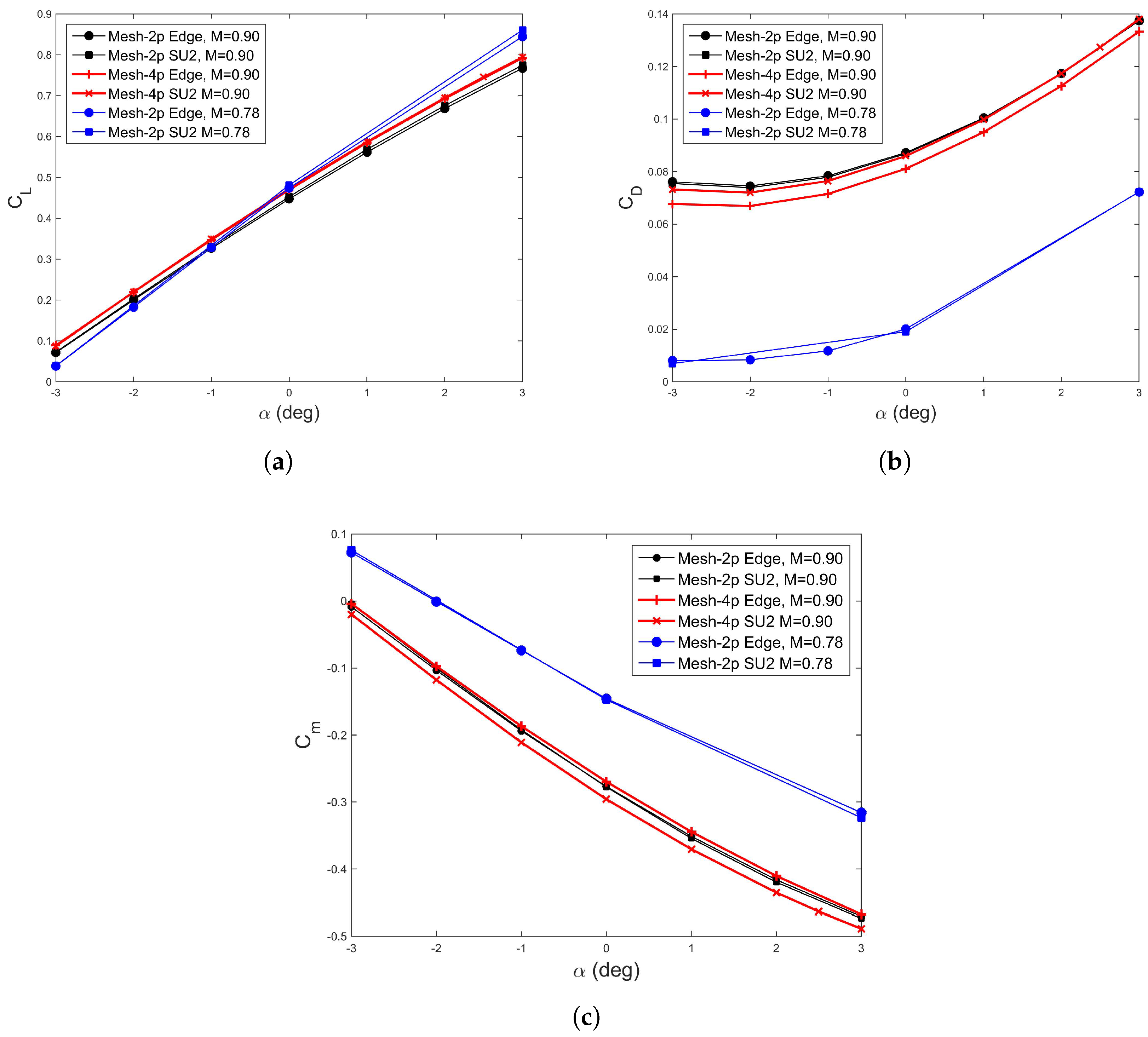
Figure 12 shows the comparison of the aerodynamic coefficients computed by Euler equations in SU2 and Edge for two different meshes of the reference aircraft. “Mesh-4p” has 4.0 million cells, and “mesh-2p” has 1.9 million cells. The meshes have the same meshing parameter settings as described in [20]. Both have refined wing leading and trailing edges, and “mesh-4p” has settings for even smaller minimum dimensions of the cells. According to the mesh study in [20], the predictions from both solvers converge as the mesh resolution increases, and “mesh-4p” was selected in [20] for all the simulations carried out by SU2 by considering both computational accuracy and efficiency. In this paper, more simulations are made for both “mesh-2p” and “mesh-4p” using both Edge and SU2 for different flight conditions. For “mesh-2p”, Edge and SU2 give fairly close predictions for the aerodynamic coefficients C L , C D and C m at Mach = 0.78 and 0.9. In the current study, we will use “mesh-4p” for the Euler solutions by SU2 in Section 5 and “mesh-2p” for the calculations on control surface modeling in Section 6, where SU2 and Edge are used to compare the geometry modeling approaches.

5. Applications

5.1. Aerodynamic Results Comparison

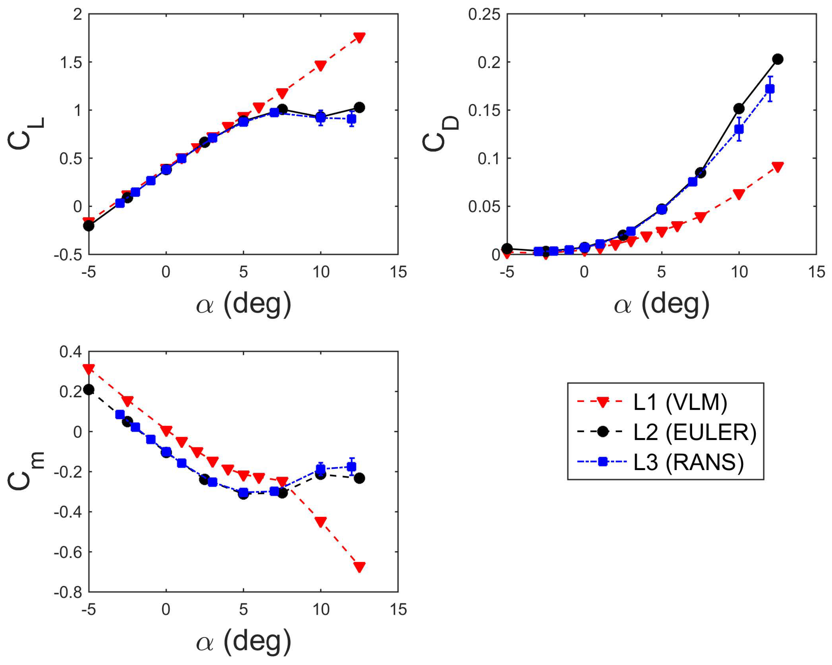
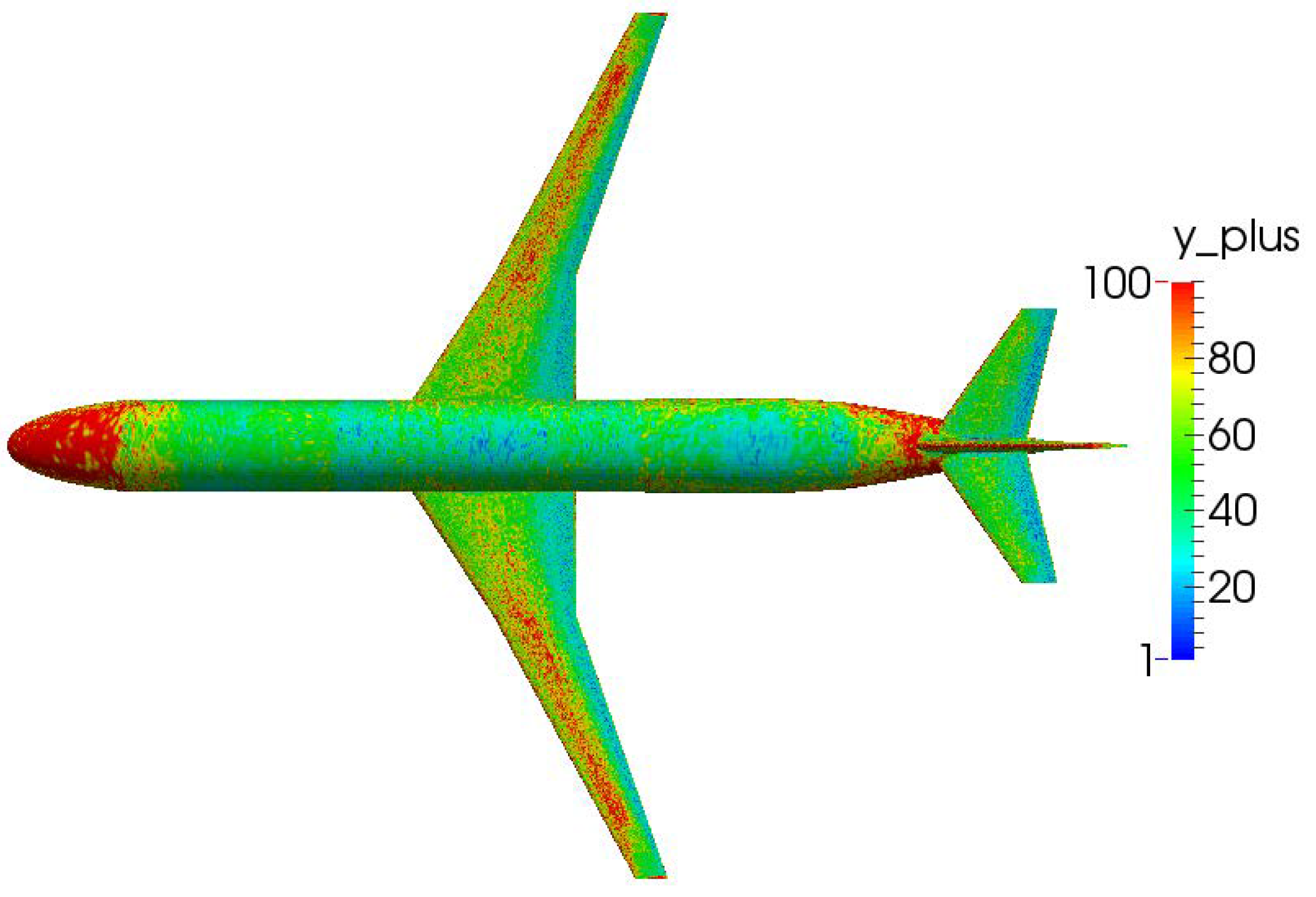
The aerodynamic coefficients obtained with L1 and L2 fidelity tools are compared in Figure 13. A Mach number of 0.6 was used to avoid transonic effects (at low angles of attack) that are not well predicted by L1 (Tornado). The flight condition used for this comparison is an altitude of 5000 m and a side slip angle β = 0 deg. The L3 (RANS) simulations for a fully-turbulent flow [33] using the Spalart–Allmaras turbulence model are also shown at the same flight condition, as the highest fidelity data for verification. The RANS mesh is generated by Pentagrow using the same Sumo surface mesh for the L2 Euler computations, which has 792,900 triangles on the surface. The RANS mesh has 8.2 million cells. The first layer height is 3.8 × 10 6 ( y + = 1 ); the growth rate is 1.2; the number of layers is 40, with the corresponding Reynolds number 32.4 million of the reference chord 3.7317 m. The airspeed is 192 m/s, which corresponds to Mach = 0.6 and altitude = 5000 m. Figure 14 shows the computed y + diagram over the reference aircraft at α = 1 with airspeed 192 m/s and Reynolds number 32.4 million.
Note that the L2 and L3 simulations agree quite well, so that we can safely assume that for this configuration under the corresponding flight conditions, L2 simulations are “as best as” the L3 simulations. In this paper, we only discuss L1 and L2 tools and their simulations. The numerical flow for α 10 is highly unsteady and is not entirely converged, the aerodynamic forces calculated by the L2 and L3 tools are the mean values of the iterations in the search of a steady flow.
The lift coefficient C L is well predicted by both L1 and L2 tools between angles of attack of −5 and +5 . Above this range, “computational” stall occurs at α of approximately 8 , which is clearly visible in the L2 results.
The drag polar shows that the minimum drag coefficient is obtained for an angle of attack of about −2.5 where C L vanishes. The minimum C D is very small with both Tornado (L1) and SU2 Euler (L2) because they do not include skin friction drag in their physical model and there is no wave drag. The L2 prediction of high C D for high angles of attack is due to wave drag. The pitching moment coefficient C m on the left corner shows that the aircraft is longitudinally stable ( C m / α < 0 ) for angles of attack from −5 to +5 . The breaks in the curves after +5 are different. For L2, it is due to “computational” stall of the horizontal stabilizer. As a reminder, this aircraft is only in the first phase of its design, so it has not been optimized in terms of stability.
The good agreement for some ranges obtained by different fidelity aerodynamic tools supports the idea of building a surrogate model trained by an automatic sampling approach that takes advantage of each method according to their fidelity levels and limitations. For example, it is useless to spend computational time with Euler calculations in the linear aerodynamic region where Tornado can give reliable results. This computational time is better spent on higher Mach number or angles of attack where the cheapest tools fail. An application of the “variable fidelity” technique is to fuse the data from different fidelity levels of tools by kriging and co-kriging [34]; see also [14].

5.2. Multi-Fidelity Aerodynamics for Data Fusion

A surrogate model with automatic sampling fuses the data obtained by the different aerodynamic tools. This is useful for constructing a look-up aero-table for quality analysis and flight simulation. This section shows which are the final surrogate models of the static aerodynamic coefficients for horizontal flight, and more results are also shown in [14]. The aircraft handling qualities are also predicted and analyzed; see the details in [14]. The multi-fidelity of the aerodynamic tools used to generate the various data for constructing the surrogate models is executed via BRICS remotely at different sites by importing/exporting the common CPACS file through the interfaces described in this paper.
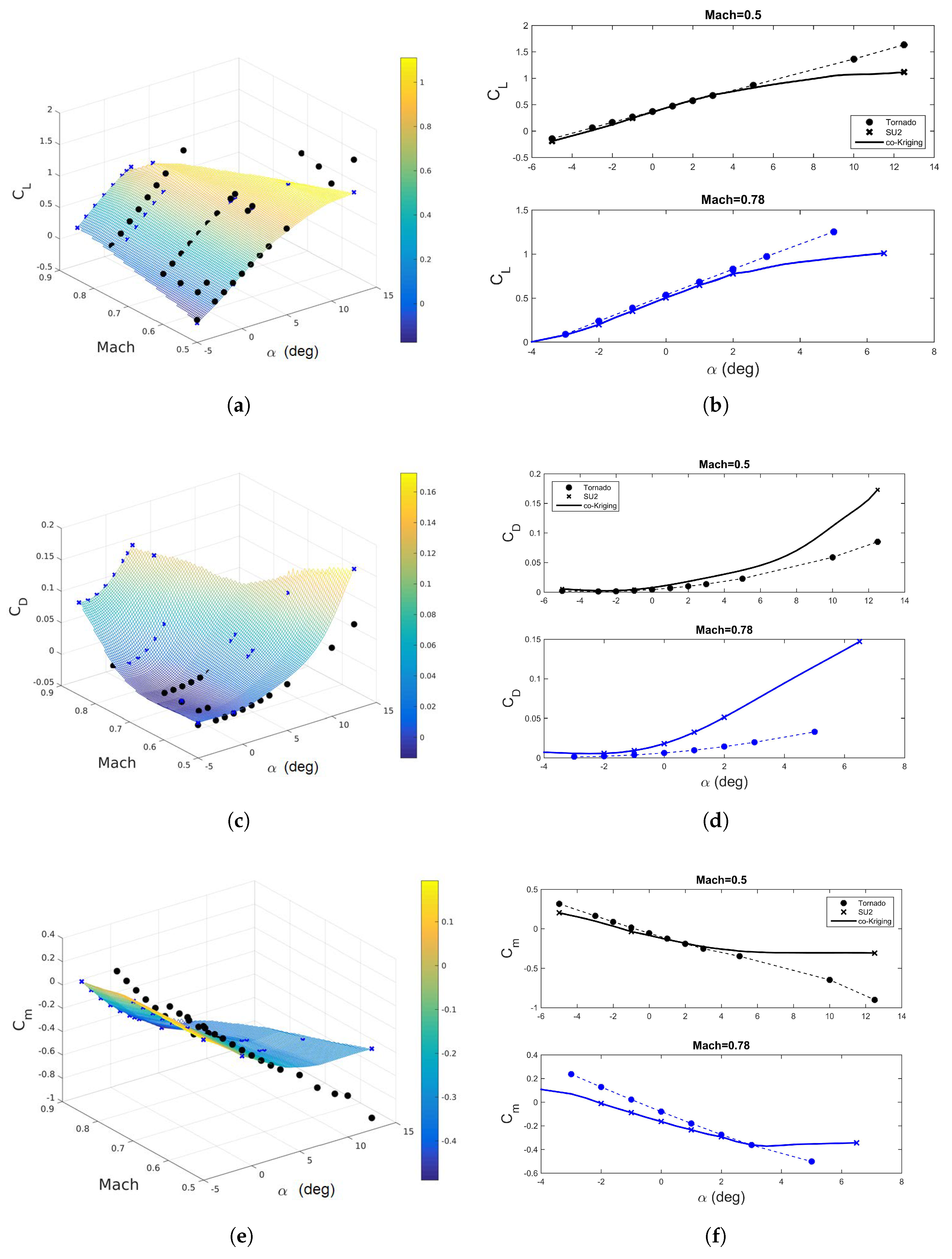
Figure 15 shows the fused C L , C D and C m aero-coefficient results of the reference aircraft model from the L1 Tornado) and L2 SU2 Euler tools with the elevator deflection δ = 0 over the flight envelope. • represents the Tornado samples, and × represents the SU2 Euler samples. Figure 15a,c,e shows the response surfaces from the surrogate models, as well as the sampled data over the flight envelope in the three-dimensional space. Figure 15b,d,f represents the variation with α and δ e for Mach numbers 0.5 (black) and 0.78 (blue) from the response surfaces and their corresponding sampled data.
Figure 15a,b shows the surrogate models (response surfaces) for C L produced by co-kriging [34]. The non-linear behavior at higher angles of attack is captured as the L2 samples indicate.
Figure 15c,d shows the prediction for C D . The surrogate model predicts higher drag than the L1 samples, since they do not predict wave drag. The surrogate model picks up the compressibility phenomena from the L2 samples.
The surrogate model for C m is shown in Figure 15e,f. Note again that the surrogate model predicts the non-linear trends at high AoA, as expected. The coarse L2 samples correct the response surfaces significantly.
The computation time of the surrogate model is ≈0.05 s on a desktop computer with four CPUs. The reliability of the surrogate as indicated by the root mean square error m a x ( RMSE ) = 0.048 < 5 % .

5.3. Aero-Data for Low Speed by the L1 Tool

Tornado computes all static and quasi-static aerodynamic coefficients, including the effects of trailing edge device deflections. In the following paragraphs, the sizing of the rudder and horizontal trim and handling qualities are discussed based on the Tornado calculations.

5.3.1. Sizing the Fin and Rudder for the One-Engine-Out Case

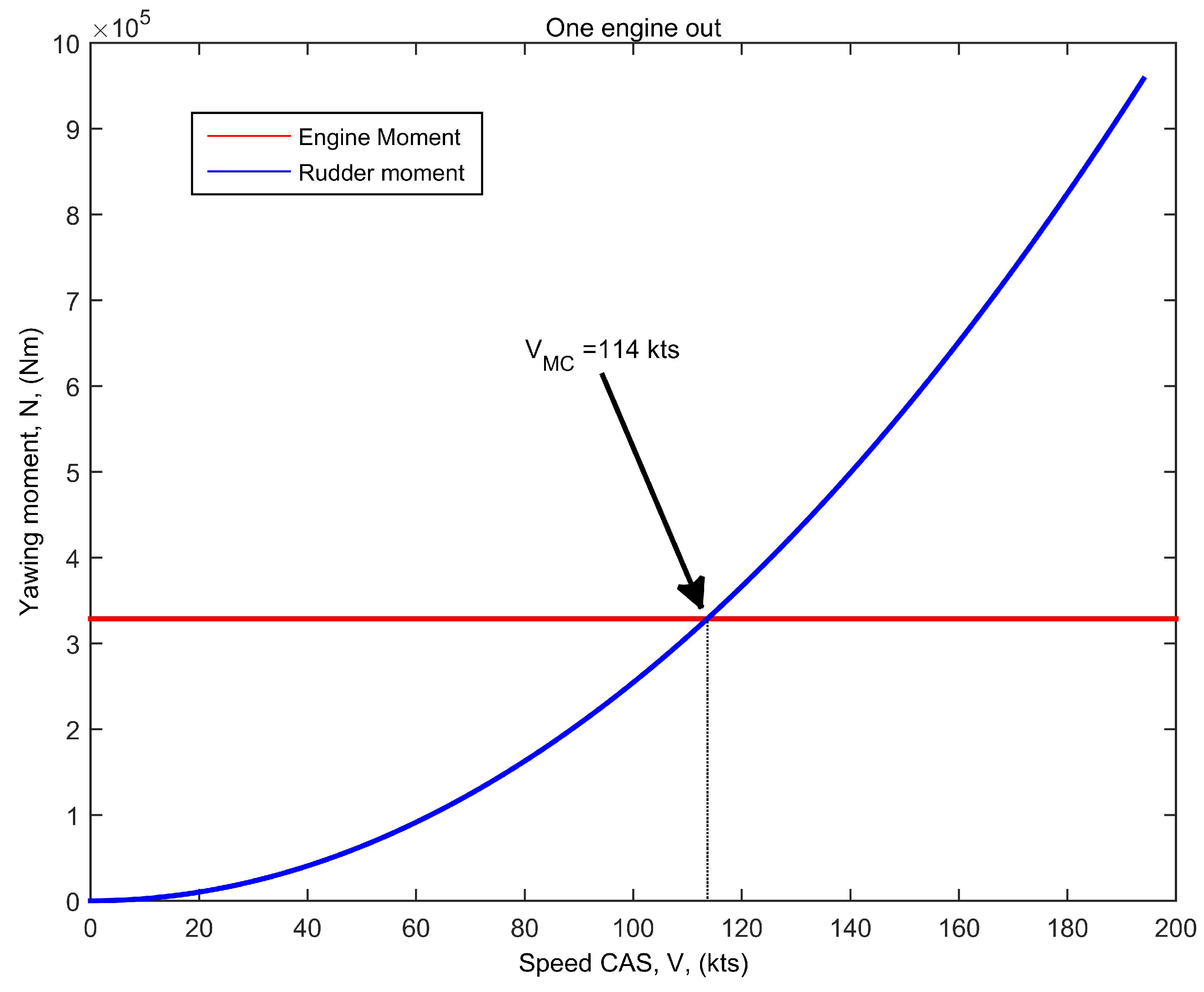
An aircraft must have an established minimum control speed V M C , legally defined in, e.g., [35], as the lowest calibrated airspeed at which the aircraft is controllable. It may not be larger than 1.13-times the reference stall speed. Aircraft with engines set far from the centerline will experience large yawing moments if an engine fails. The sizing of the vertical tail, and its rudder, is usually determined by a one-engine-out case. Flying with side-slip and rudder deflection, at a certain airspeed, the fin and rudder produce just enough yawing moment to counteract the asymmetric thrust. This speed is essentially the minimum control speed, although certification requires a few more parameters.
In this section, an exercise of sizing the rudder of the aircraft is carried out by Tornado, using a simplified method as described by Torenbeek [36]. Side-slip and roll response were neglected, and the tail volume [37] was held constant.
As an initial estimate, the minimum control speed for different control surface sizes was computed until the requirement of 1.13 of the stall speed was achieved. The selected rudder deflection was 25 degrees to allow five degrees of maneuver margin. Figure 16 shows the predicted minimum control velocity.

5.3.2. Handling Qualities

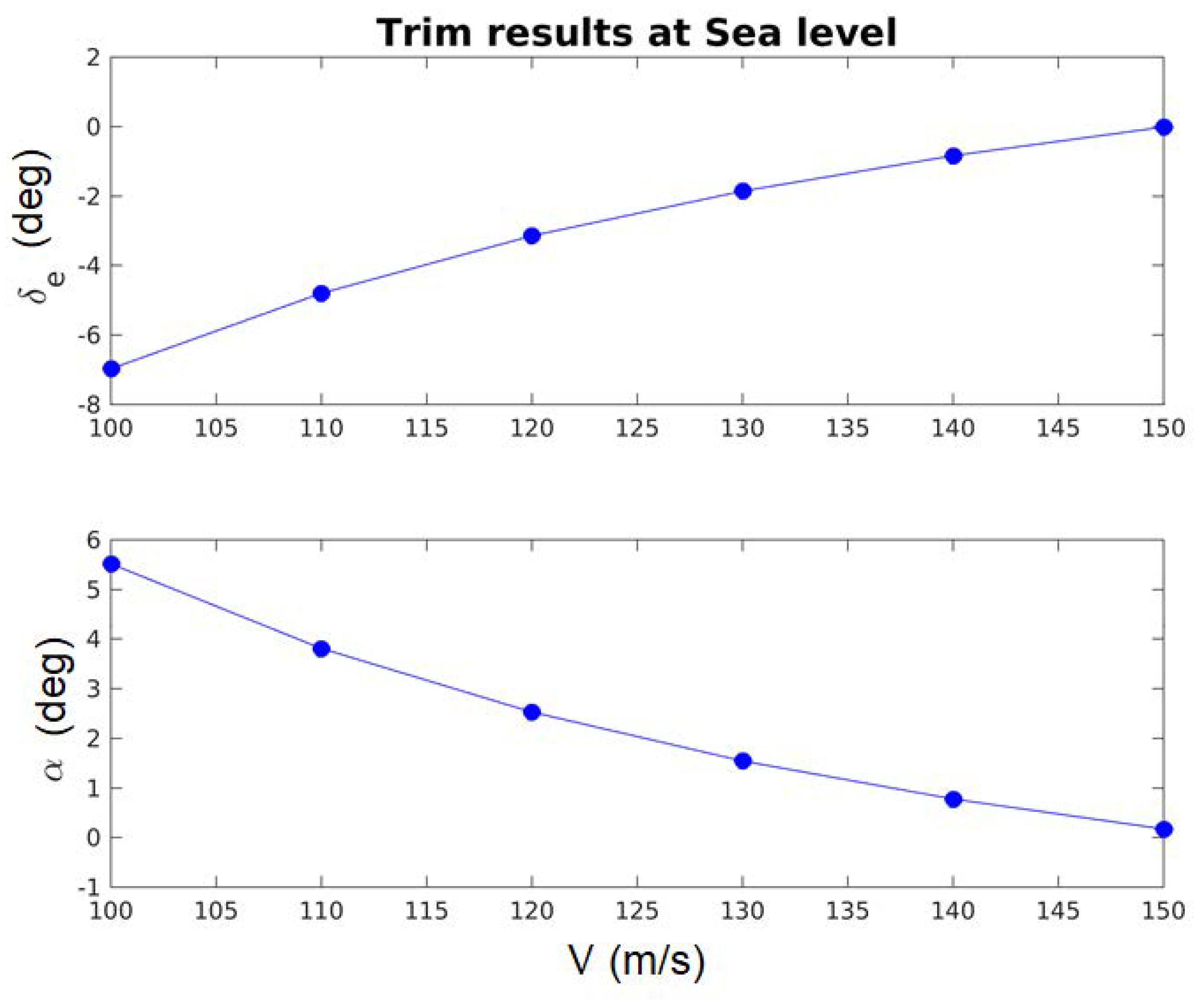
The horizontal sea level trim at low speed can be estimated from the aero-coefficients and the mass distribution whose reference values are available from CPACS. The straight and level flight trim results at sea level, calculated by Tornado in [20] are shown in Figure 17.
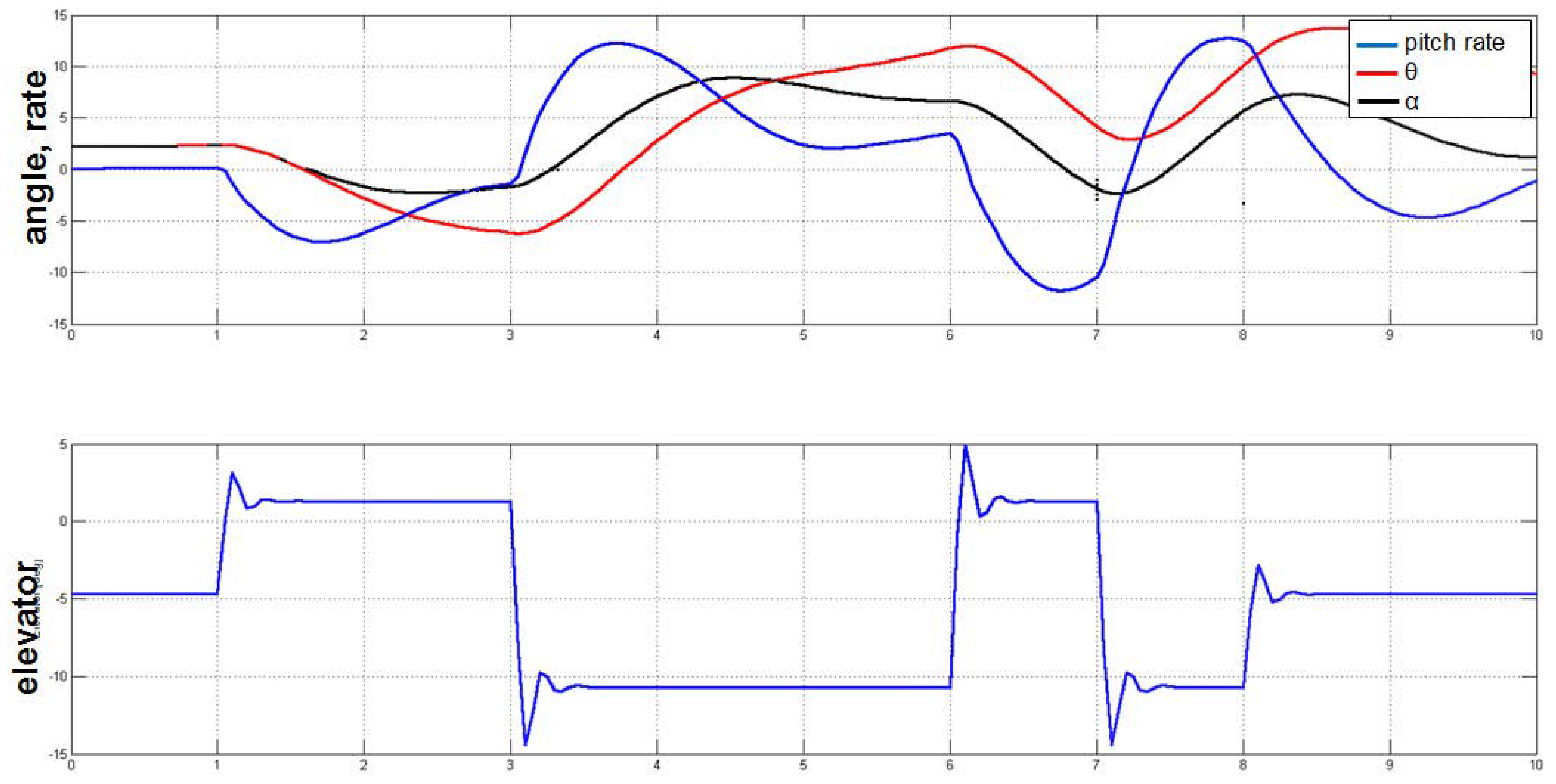
The classical modes of motion indicate the linear stability of the aircraft, i.e., its responses to (infinitesimally) small disturbances. Flight simulation allows the full range of stability of the aircraft to be assessed. The time history in Figure 18 shows how the attitude angle θ , the angle of attack α and the pitch rate q oscillate when excited by a step-function-type elevator movement. The PHALANX [1,2,3,4,38], a flight simulation tool from Delft University of Technology, produced the time histories.
The time domain simulation starts as trimmed straight and level flight at sea level conditions with True Air Speed 130 m/s. After 1 s, the pilot executes a 2-3-1-1 maneuver in pitch, namely, stick 2 s nose down, 3 s nose up, 1 s nose down and 1 s nose up.

6. Euler Computation for Various Control Surface Models

Analysis for control surface deflection is an important capability of L2-3 CFD tools. In this section, elevator deflection by mesh deformation, morphing trailing edge shape and transpiration boundary conditions are described. Euler results by different flow solvers are compared. The surfaces are deflected by deforming the surfaces, and no gaps are modeled.

6.1. Modeling Movable Surfaces

SU2 uses a mesh deformation defined by a set of control points for a Free-Form Deformation (FFD) box [39], thus only the clean configuration mesh is generated from scratch. The SU2_DEF built-in mesh deformation function is then used to deform the mesh around the elevator locations on the horizontal tail (see Figure 19a). An FFD box is defined at the elevator locations. The FFD box of control points can be rotated around the hinge line. Owing to the affine invariance of the map from control points to the mesh, the surface mesh follows. According to the authors’ experience, with a deflection of less than eight degrees, the deformed mesh is still well formed enough to function for Euler simulation isotropic grids.
It is also possible to morph the shape, represented by control point technology, and re-generate the mesh for each deflection. Auto-morphing scripts (re-)generating the surface grids with deflected control surface(s) in Sumo are described in [40].
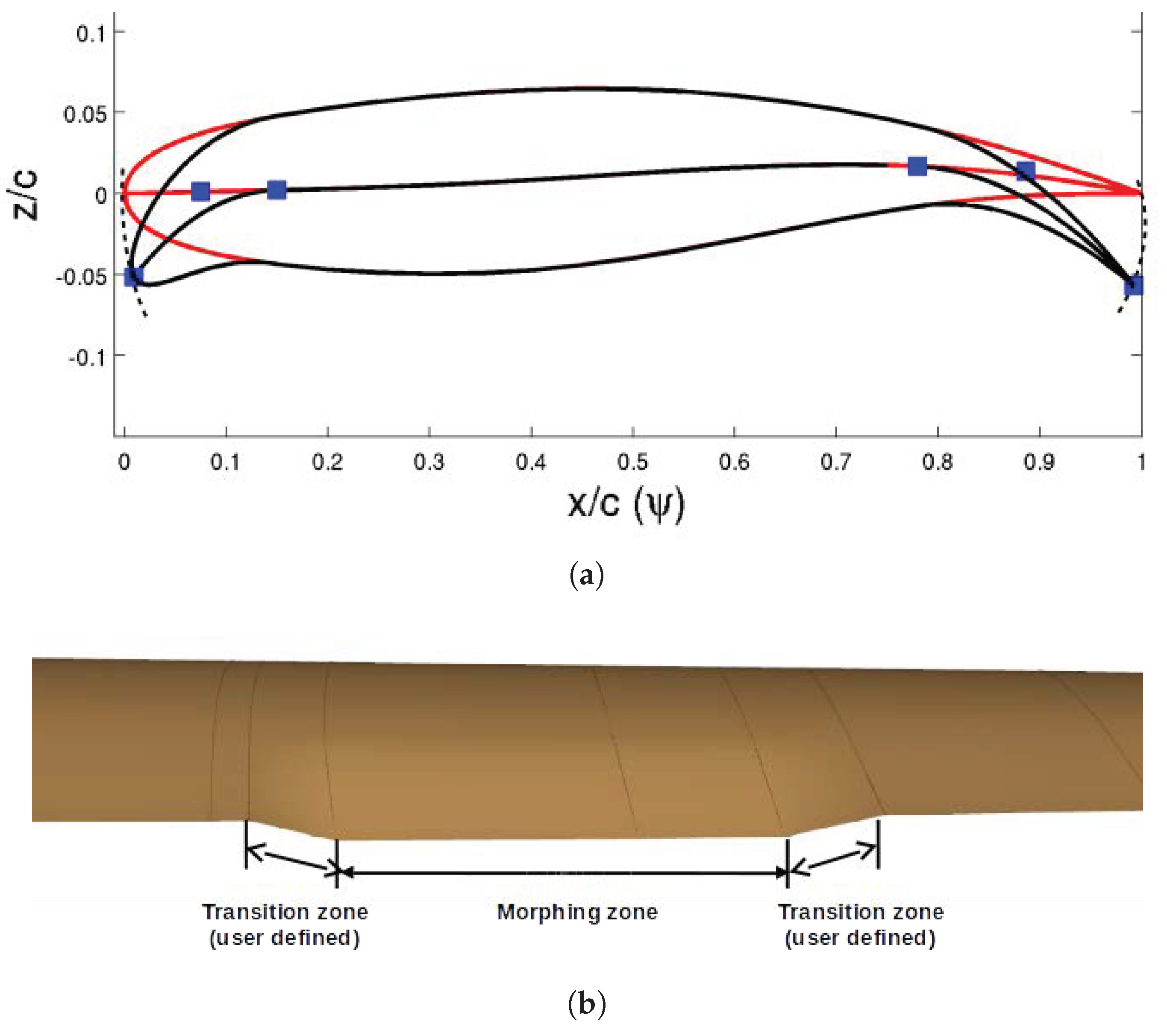
The Trailing Edge (TE) morphing starts by extracting the camber curve and thickness distribution from the airfoil data [40]. The auto-morphing scripts create new sections (as required) at control surface edges. The new section camber curves are morphed according to the deflection angle, to which the thickness is added. Figure 20a illustrates the camber controlled by quadratic Bézier curves for morphed leading and trailing edges with the thickness distribution preserved. The quadratic Bézier control points are chosen to give (at least) G1-continuity of the deformed camber curves. Issues related to crossing of camber curve normals close to control surface edges must be addressed. The camber curves for morphed leading and trailing edges are based on the Class–Shape function Transformation (CST) approach [41]. It enables easy geometry manipulation by user-defined parameters such as the hinge line, rotation angle and the transition zones; see Figure 20b.
Figure 19b shows the Sumo surface mesh for a deflection angle of six degrees. Both mesh deformation by FFD (Figure 19a) and morphing of the camber lines produce gapless meshes according to the control surface deflections. The morphing technology in addition supports a user-defined transition zone (length and type) to obtain a smoother surface and avoid bad tetrahedral cells. The smooth transition feature makes the trailing edge morphing technology possible for a RANS simulation; however, the mesh deformation by FFD tends to produce high aspect ratio cells at the deformed junctions, so the mesh may work well only for coarser Euler simulations.
Edge calculates the aerodynamics of control surface deflections by transpiration boundary conditions. The grid does not move; only the normals used in the no-flow boundary condition are deflected; see Figure 19c.

6.2. Results Comparison

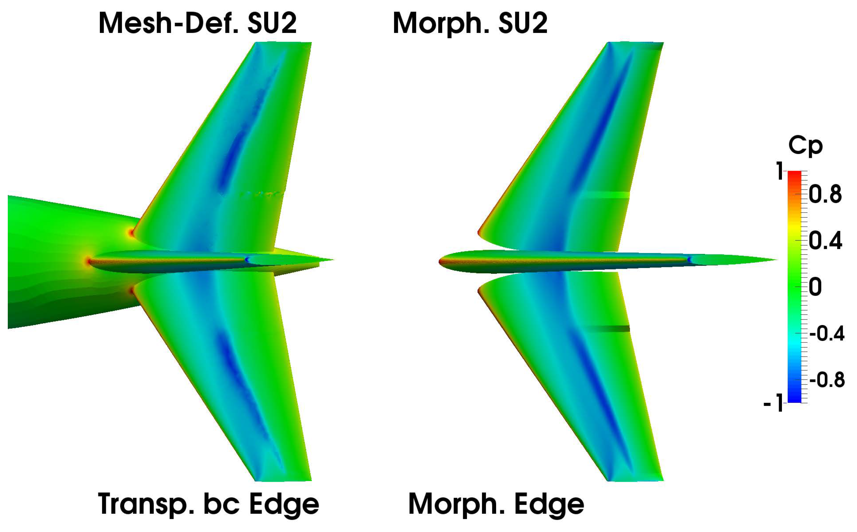
This section shows the results of the control surface modeling approaches with different CFD solvers. Figure 21 and Table 1 show the comparisons for C L , C m and their derivatives for elevator deflection ± 6 , at Mach 0.78, altitude 10,000 m, α = 0 . We expect close agreement for morphing elevators computed by SU2 and Edge, by mesh deformation, as well as morphing. The solutions for mesh deformation by SU2 FFD and transpiration boundary condition by Edge are quite comparable. The morphing control surface model predicts slightly higher slopes for both C L and C m and a smoother flow on the horizontal tail (see Figure 22), probably due to the transition part of the morphed shape. Note that the transition zone as defined in this case gives a slightly larger deflected area.
Note that the abbreviations used in Table 1, Figure 21 and Figure 22 are:
  • Mesh-Def(orm): Mesh deformation using FFD;
  • Morph. (cs): Morphing the control surfaces by Sumo;
  • Transp. b.c.: transpiration boundary conditions in Edge.

7. Conclusions

Seamless connection by the CPACS data schema enables integration and implementation of variable fidelity tools into the aircraft design multi-disciplinary analysis and optimization workflow. This paper presents L1 and L2 fidelity aerodynamic design tools using auto-meshing. Applications to the defined test case aircraft includes aerodynamic analysis, data fusion of variable fidelity data and handling quality analysis by flight simulation. A comprehensive discussion is given of different models for control surface deflections for Euler computation.

Author Contributions

Mengmeng Zhang developed the CPACS-Tornado interface and made the corresponding calculations, carried out the Euler calculations by SU2 and Edge for solver comparisons and for the control surface model analyses, analyzed the data and wrote the paper. Aidan Jungo developed the CPACS2SUMO interface, carried out the Euler calculations by SU2 and wrote the corresponding part of the paper and the CPACS description. Alessandro Augusto Gastaldi developed the PyTornado, wrote the corresponding part of the paper and helped write the paper. Tomas Melin carried out the Tornado calculations for sizing the fin and rudder and wrote the corresponding part of the paper.

Acknowledgments

The research presented in this paper has been performed in the framework of the AGILE project (Aircraft 3rd Generation MDO for Innovative Collaboration of Heterogeneous Teams of Experts) and has received funding from the European Union Horizon 2020 Programme (H2020-EU.3.4) under Grant Agreement No. 636202. The Swiss participation in the AGILE project was supported by the Swiss State Secretariat for Education, Research and Innovation (SERI) under Contract Number 15.0162. The authors are grateful to the partners of the AGILE consortium for their contributions and feedback; Mark Voskuijl, Delft University of Technology, for the flight simulation analysis from PHALANX; Jesper Oppelstrup, Royal Institute of Technology (KTH), Sweden, for the valuable comments and suggestions.

Conflicts of Interest

The authors declare no conflict of interest. The sponsors had no role in the design of the study; in the collection, analyses or interpretation of data; in the writing of the manuscript; nor in the decision to publish the results.

Abbreviations

AGILEAircraft 3rd Generation MDO for Innovative Collaboration of Heterogeneous Teams of Experts
APIApplication Programming Interface
CADComputer Aided Design
CFDComputational Fluid Dynamics
CPACSThe Common Parametric Aircraft Configuration Schema
CSTClass-Shape function Transformation
DESDetached Eddy Simulation
FFDFree-Form Deformation
GUIGraphic User Interface
LESLarge-Eddy Simulation
MACMean Aerodynamic Chord
MDAMultidisciplinary Analysis
MDOMultidisciplinary Design and Optimization
RANSReynolds-Averaged Navier–Stokes equations
TASTrue Air Speed
TE(D)Trailing Edge (Device)
UIUser Interface
VLMVortex Lattice Method
XMLExtensible Markup Language
Symbols
α or AoAAngle of Attack (deg)
δ e Elevator deflection angle (deg)
θ Attitude angle (deg)
qPitch rate (deg/s)
C p Pressure Coefficient (-)
C L Lift coefficient (-)
C D Drag coefficient (-)
C m Pitching moment coefficient (-)

References

  1. Voskuijl, M.; de Klerk, J.; van Ginneken, D. Flight Mechanics Modelling of the Prandtl Plane for Conceptual and Preliminary Design; Springer: London, UK, 2012; Volume 66. [Google Scholar]
  2. Voskuijl, M.; La Rocca, G.; Dircken, F. Controllability of blended wing body aircraft. In Proceedings of the 26th Congress of International Council of the Aeronautical Sciences, Anchorage, AK, USA, 14–19 September 2008. [Google Scholar]
  3. Fengnian, T.; Voskuijl, M. Automated Generation of Multiphysics Simulation Models to Support Multidisciplinary Design Optimization. Adv. Eng. Inform. 2015, 29, 1110–1125. [Google Scholar]
  4. Foeken, M.J.; Voskuijl, M. Knowledge-Based Simulation Model Generation for Control Law Design Applied to a Quadrotor UAV. Math. Comput. Model. Dyn. Syst. 2010, 16, 241–256. [Google Scholar] [CrossRef]
  5. Raymer, D. Conceptual design modeling the RDS-professional aircraft design software. In Proceedings of the AIAA Aerospace Sciences Meeting, Orlando, FL, USA, 4–7 January 2011. [Google Scholar]
  6. Anemaat, W.A.; Kaushik, B. Geometry design assistant for airplane preliminary design. In Proceedings of the 49th AIAA Aerospace Sciences Meeting including the New Horizons Forum and Aerospace Exposition, Orlando, FL, USA, 4–7 January 2011. [Google Scholar]
  7. Gloudemans, J.R.; Davis, P.C.; Gelausen, P.A. A rapid geometry modeler for conceptual aircraft. In Proceedings of the 34th AIAA Aerospace Sciences Meeting and Exhibit, Reno, NV, USA, 15–18 January 1996. [Google Scholar]
  8. Tomac, M. Towards Automated CFD for Engineering Methods in Aircraft Design. Ph.D. Thesis, Royal Institute of Technology, KTH, Stockholm, Sweden, 2014. [Google Scholar]
  9. CPACS—A Common Language for Aircraft Design. Available online: http://www.cpacs.de/ (accessed on 7 February 2018).
  10. Böhnke, D.; Nagel, B.; Zhang, M.; Rizzi, A. Towards a collaborative and integrated set of open tools for aircraft design. In Proceedings of the 51st AIAA Aerospace Sciences Meeting including the New Horizons Forum and Aerospace Exposition, Grapevine, TX, USA, 7–10 January 2013; pp. 7–10. [Google Scholar]
  11. SUAVE—An Aerospace Vehicle Environment for Designing Future Aircraft. Available online: http://suave.stanford.edu/ (accessed on 20 March 2018).
  12. Lukaczyk, T.; Wendorff, A.; Botero, E.; MacDonald, T.; Momose, T.; Variyar, A.; Vegh, J.M.; Colonno, M.; Economon, T.; Alonso, J.J.; et al. SUAVE: An Open-Source Environment for Multi-Fidelity Conceptual Vehicle Design. In Proceedings of the 16th AIAA Multidisciplinary Analysis and Optimization Conference, Dallas, TX, USA, 22–26 June 2015. [Google Scholar]
  13. MacDonald, T.; Clarke, M.; Botero, E.M.; Vegh, J.M.; Alonso, J.J. SUAVE: An Open-Source Environment Enabling Multi-fidelity Vehicle Optimization. In Proceedings of the 18th AIAA Multidisciplinary Analysis and Optimization Conference, Denver, CO, USA, 5–9 June 2017. [Google Scholar]
  14. Zhang, M.; Bartoli, N.; Jungo, A.; Lammen, W.; Baalbergen, E. Data Fusion and Aerodynamic Surrogate Modeling for Handling Qualities Analysis. Prog. Aerosp. Sci. Spec. Issue 2018. submitted. [Google Scholar]
  15. AGILE EU Project Portal. Available online: http://www.agile-project.eu (accessed on 15 January 2018).
  16. Seider, D.; Fischer, P.; Litz, M.; Schreiber, A.; Gerndt, A. Open Source Software Framework for Applications in Aeronautics and Space. In Proceedings of the IEEE Aerospace Conference, Big Sky, MT, USA, 3–10 March 2012. [Google Scholar]
  17. Baalbergen, E.; Kos, J.; Louriou, C.; Campguilhem, C.; Barron, J. Streamlining cross-organisation product design in aeronautics. Proc. Inst. Mech. Eng. Part G J. Aerosp. Eng. 2016. [Google Scholar] [CrossRef]
  18. Moerland, E.; Ciampa, P.D.; Zur, S.; Baalbergen, E.; D’Ippolito, R.; Lombardi, R. Collaborative Architecture supporting the next generation of MDO within the AGILE Paradigm. Prog. Aerosp. Sci. Spec. Issue 2018. submitted. [Google Scholar]
  19. Van Gent, I.; Aigner, B.; Beijer, B.; Jepsen, J.; Rocca, G.L. Knowledge architecture supporting the next generation of MDO in the AGILE paradigm. Prog. Aerosp. Sci. Spec. Issue 2018. submitted. [Google Scholar]
  20. Jungo, A.; Vos, J.; Zhang, M.; Rizzi, A. Benchmarkig New CEASIOM with CPACS Adoption for Aerodynamic Analysis and Flight Simulation. Aircr. Eng. Aerosp. Technol. 2017, 90. [Google Scholar] [CrossRef]
  21. TIGL—Geometry Library to Process Aircraft Geometries in Pre-Design. Available online: https://github.com/DLR-SC/tigl (accessed on 30 November 2017).
  22. CPACS Documentation. Available online: https://github.com/DLR-LY/CPACS/tree/develop/documentation (accessed on 20 April 2018).
  23. Melin, T. Using Internet Interactions in Developing Vortex Lattice Software for Conceptual Design. Ph.D. Thesis, Department of Aeronautics, Royal Institute of Technology, KTH, Stockholm, Sweden, 2003. [Google Scholar]
  24. Tomac, M.; Eller, D. From Geometry to CFD Grids: An Automated Approach for Conceptual Design. Prog. Aerosp. Sci. 2011, 47, 589–596. [Google Scholar] [CrossRef]
  25. Si, H. TetGen: A Quality Tetrahedral Mesh Generator and 3D Delaunay Triangulator; Technical Report, User’s Manual; Technical Report No. 13; Numerical Mathematics and Scientific Computing, Weierstrass Institute for Applied Analysis and Stochastics (WIAS): Berlin, Germany, 2013. [Google Scholar]
  26. Anderson, J.D. Modern Compressible Flow with Historical Perspective, 3rd ed.; McGraw-Hill: New York, NY, USA, 2004. [Google Scholar]
  27. Katz, J.; Plotkin, A. Low-Speed Aerodynamics: From Wing Theory to Panel Methods; McGraw-Hill, Inc.: New York, NY, USA, 1991. [Google Scholar]
  28. Eliasson, P. Edge, a Navier-Stokes Solver for Unstructured Grids. In Finite Volumes for Complex Applications III; Elsevier: Amsterdam, The Netherlands, 2002; pp. 527–534. [Google Scholar]
  29. Palacios, F.; Colonno, M.R.; Aranake, A.C.; Campos, A.; Copeland, S.R.; Economon, T.D.; Lonkar, A.K.; Lukaczyk, T.W.; Taylor, T.W.R.; Alonso, J. Stanford University Unstructured (SU2): An open-source integrated computational environment for multi-Physics simulation and design. In Proceedings of the 51st AIAA Aerospace Sciences Meeting including the New Horizons Forum and Aerospace Exposition, Grapevine, TX, USA, 7–10 January 2013. AIAA 2013-0287. [Google Scholar]
  30. Economon, T.D.; Palacios, F.; Copeland, S.R.; Lukaczyk, T.W.; Alonso, J.J. SU2: An Open-Source Suite for Multiphysics Simulation and Design. AIAA J. 2015, 54, 828–846. [Google Scholar] [CrossRef]
  31. Palacios, F.; Economon, T.D.; Wendorff, A.D.; Alonso, J. Large-Scale Aircraft Design Using SU2. In Proceedings of the 53rd AIAA Aerospace Sciences Meeting, AIAA 2015-1946, Kissimmee, FL, USA, 5–9 January 2015. [Google Scholar]
  32. Griva, I.; Nash, S.G.; Sofer, A. Linear and Nonlinear Optimization, 2nd ed.; Society for Industrial Applied Mathematics: Philadelphia, PA, USA, 2009. [Google Scholar]
  33. Yousefi, K.; Razeghi, A. Determination of the Critical Reynolds Number for Flow over Symmetric NACA Airfoils. In Proceedings of the 2018 AIAA Aerospace Sciences Meeting, AIAA 2018–0818, Kissimmee, FL, USA, 8–12 January 2018. [Google Scholar]
  34. Forrester, A.; Keane, A. Engineering Design via Surrogate Modelling: A Practical Guide; John Wiley & Sons: Hoboken, NJ, USA, 2008. [Google Scholar]
  35. Federal Aircraft Administration. CFR 25.149; Technical Report, Retrieved 18 January 2018; Federal Aircraft Administration: Washington, DC, USA, 2018.
  36. Torenbeek, E. Synthesis of Subsonic Airplane Design; Delft University Press: Delft, The Netherlands, 1982. [Google Scholar]
  37. Etkin, B.; Reid, L.D. Dynamics of Flight: Stability and Control; John Wiley & Sons: Hoboken, NJ, USA, 1996. [Google Scholar]
  38. Pfeiffer, T.; Nagel, B.; Böhnke, D.; Voskuijl, M.; Rizzi, A. Implementation of a Heterogeneous, Variable-Fidelity Framework for Flight Mechanics Analysis in Preliminary Aircraft Design; Deutscher Luft-und Raumfahrtkongress: Bremen, Germany, 2011. [Google Scholar]
  39. Sederberg, T.W.; Parry, S.R. Free-Form Deformation of Solid Geometric Models. In Proceedings of the SIGGRAPH ’86 13th Annual Conference on Computer Graphics and Interactive Techniques, Atlanta, GA, USA, 1–5 August 1986; Volume 20, pp. 151–160. [Google Scholar]
  40. Zhang, M. Contributions to Variable Fidelity MDO Framework for Collaborative and Integrated Aircraft Design. Ph.D. Thesis, Royal Institute of Technology KTH, Stockholm, Sweden, 2015. [Google Scholar]
  41. Kulfan, B. Universal Parametric Geometry Representation Method. J. Aircr. 2008, 45, 142–158. [Google Scholar] [CrossRef]
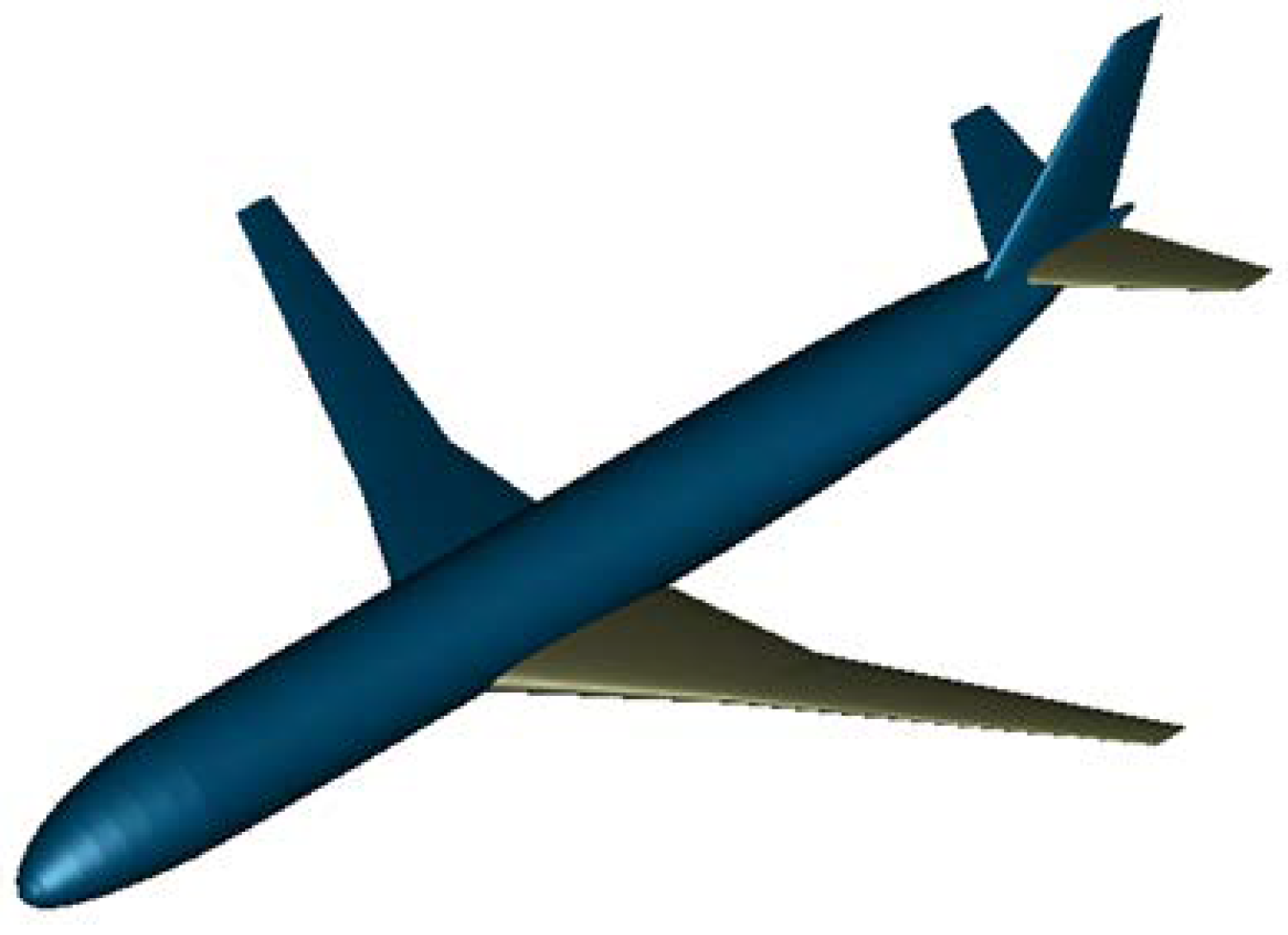
Figure 1. The reference aircraft, rendered by the CPACS visualization tool TIGLViewer [21].
Aerospace 05 00047 g001
Figure 2. The airfoil details of the reference aircraft. (a) The airfoils of the reference aircraft; (b) the thickness and camber information of the airfoils.
Aerospace 05 00047 g002
Figure 3. The CPACS hierarchical structure (image from the CPACS website [9]).
Aerospace 05 00047 g003
Figure 4. Adapted from CPACS documentation [9]; schema for the construction of an aircraft wing from its XML file definition.
Aerospace 05 00047 g004
Figure 5. CPACS trailing edge device definition for node outerShape [9,22].
Aerospace 05 00047 g005
Figure 6. Tornado partition layout with control surfaces for the reference aircraft, imported from CPACS.
Aerospace 05 00047 g006
Figure 7. Panel distributions and the C p visualization in PyTornado for a box-wing aircraft, imported from CPACS. (a) Panel layout; (b) the C p simulation for U = 100 m/s, α = 5 .
Aerospace 05 00047 g007
Figure 8. Tornado program workflow: user interface in Python and the core functions in C++.
Aerospace 05 00047 g008
Figure 9. The surface and volume meshes of the reference aircraft generated by Sumo with TetGen and Pentagrow. (a) Sumo surface mesh; (b) Sumo-Pentagrow RANS mesh.
Aerospace 05 00047 g009
Figure 10. Sumo creates a wing from a stack of airfoils.
Aerospace 05 00047 g010
Figure 11. Schema to construct an aircraft from its Sumo XML file format.
Aerospace 05 00047 g011
Figure 12. Euler simulations for the reference aircraft for C L , C D and C m computed by Edge and SU2 for meshes “mesh-2p” and “mesh-4p”, at a flight altitude of 10,000 m, Mach 0.78 and Mach 0.9 respectively. (a) Lift coefficient C L for Mach number of 0.78 and 0.9; (b) drag coefficient C D for Mach numbers of 0.78 and 0.9; (c) pitching moment coefficient C m for Mach numbers of 0.78 and 0.9.
Aerospace 05 00047 g012
Figure 13. L1, L2 and L3 simulations for the test case aircraft, α sweep at Mach = 0.6, altitude = 5000 m and β = 0 .
Aerospace 05 00047 g013
Figure 14. The y + diagram over the reference aircraft at α = 1 with airspeed 192 m/s and Reynolds number 32.4 million.
Aerospace 05 00047 g014
Figure 15. Surrogate model results of the reference aircraft for C L , C D and C m , with no elevator deflection. Notations: dot: Tornado (L1) samples; cross: SU2 (L2) Euler samples; line: the response surfaces. (a,c,e) The response surfaces and sampled data over the flight envelope. (b,d,f) The cuts for Mach number 0.5 (black) and 0.78 (blue) from the response surfaces and their corresponding sampled data; the results are also shown in [14]. (a) Lift coefficient C L surface and the sampled data; (b) fused lift coefficient C L for Mach numbers of 0.5 and 0.78; (c) drag coefficient C D surface and the sampled data; (d) fused drag coefficient C D for Mach numbers of 0.5 and 0.78; (e) pitching moment coefficient C m surface and the sampled data; (f) fused pitching moment coefficient C m for Mach 0.5 and 0.78.
Aerospace 05 00047 g015
Figure 16. Computed minimum control speed V M C , from Tornado solutions.
Aerospace 05 00047 g016
Figure 17. Trimmed angle of attack and elevator deflection at sea level, from Tornado solutions.
Aerospace 05 00047 g017
Figure 18. Flight time domain simulation from PHALANX, trimmed flight with True Air Speed (TAS) = 130 m/s at sea level.
Aerospace 05 00047 g018
Figure 19. The mesh generated by Sumo with different modeling technologies to be computed for elevator deflection at 6 . (a) Surface mesh with mesh deformed by FFD on the elevator for δ e = 6 degrees; (b) surface mesh with morphed elevator modeled by Sumo for δ e = 6 degrees, which includes a linear type 5% transition zone of the morphing elevator length; (c) tailplane and the elevators marked in the surface mesh in Sumo.
Aerospace 05 00047 g019
Figure 20. The demonstration of the automatically gapless movable surfaces morphing technology by Sumo. (a) The geometric parameters describing the morphing airfoil [40], morphing leading edge and trailing edge and a fixed central area using a variable camber; (b) illustration of the morphing trailing edge with the morphing zone and transition zones modeled in Sumo.
Aerospace 05 00047 g020
Figure 21. Euler solutions for elevator deflection δ e = 6 at Mach 0.78, flight altitude 10,000 m, α = 0 , by three control surface modeling methods, for SU2 and Edge.
Aerospace 05 00047 g021
Figure 22. C p contours of Euler solutions for the elevator deflection δ e = 6 at Mach 0.78, flight altitude 10,000 m, α = 0 , by three control surface modeling methods, SU2 and Edge.
Aerospace 05 00047 g022
Table 1. Result for different modeling of elevator deflections using different solvers, at Mach 0.78, flight altitude 10,000 m, α = 0 .
Model TypeSolver C L , δ (deg) C m , δ (deg)
Mesh-deformSU20.0092−0.0399
Morph. csSU20.0130−0.0565
Morph. csEdge0.0117−0.0557
Transp. b.c.Edge0.0095−0.0411