Article

An Efficient Processing Architecture for Range Profiling Using Noise Radar Technology

by
Davide Massaro
1,2,*,
Riccardo Ardoino
2,† and
Marco Grazzini
2,†
1
Department of Electronic Engineering, University of Rome “Tor Vergata”, via del Politecnico 1, 00133 Rome, Italy
2
System Analysis Group, Elettronica SpA, via Tiburtina Valeria km 13,700, 00133 Rome, Italy
*
Author to whom correspondence should be addressed.
These authors contributed equally to this work.
Aerospace 2018, 5(1), 4; https://doi.org/10.3390/aerospace5010004
Submission received: 4 November 2017 / Revised: 24 December 2017 / Accepted: 3 January 2018 / Published: 6 January 2018
(This article belongs to the Special Issue Radar and Aerospace)

Abstract

:
The importance of high resolution range profiles (HRRPs) for radar applications like tracking or classification is well known. In the scientific literature several approaches have been investigated to obtain HRRPs from wideband radar signals. Recent works show that noise radar waveforms can be exploited in this sense due to their high resolution and low peak to sidelobe ratio (PSLR) properties. However their use can cause some issues in applications where long time integrations are required, e.g., in the presence of a low effective radiated power (ERP) transmitter: recording the reference signal in this case would be difficult due to the big quantity of data. This work proposes a real time digital processing schematic based on linear feedback shift registers (LFSRs) which is very flexible and has a low computational burden: its internal state can be easily controlled and reproduced in reception, where a multichannel correlator is exploited as matched filter. The resulting signal, compared to typical “pulse compression” and noise radar waveforms, shows similar performances but a lower order of complexity in terms of real time generation and reception.

1. Introduction

The capability of identifying unknown targets has become a fundamental aspect that the military world needs to investigate: in fact, the effectiveness of a mission can often depend on a rapid and reliable identification process, fundamental to recognize the threats or to avoid the so called “friendly fire” [1].
In this context, the use of high resolution range profiles (HRRPs) represents a challenging topic which has been investigated in the scientific literature both for maritime and for airborne targets: in fact, as well as their employment in search and tracking applications, various works exploited HRRPs also for classification/identification purposes [2,3,4,5,6,7]. They can provide information about radar targets when 2-D imaging techniques fail; the latter, in fact, might show a series of issues in particular situations, e.g., when a synthetic aperture radar (SAR) cannot be installed on a moving sensor platform or when an inverse-SAR (ISAR) system finds difficulties in determining an axis rotation for slow targets. Some studies (e.g., [5]), also suggest that HRRPs are quite robust against aspect angle variations of the target.
HRRPs convey the information about a target, hence the waveforms exploited to perform this task have a great importance; high range resolution techniques rely, in general, on wideband waveforms. The latter include short pulses, compressed pulses and synthetic bandwidth signals [5].
Simple pulse systems require short signals to achieve high range resolution, but, as the duration of the pulse decreases, the transmitted power must be increased in order to maintain the same signal to noise ratio (SNR) conditions (the pulse duration is directly related to the energy transmitted). For the aforementioned reason, a simple pulse suffers from high power requirements or limited detection [8,9].
Pulse compressed waveforms allow to solve the problem that afflicts simple short-pulses. This class of signals is extensively used, providing high resolution without the compromise energy/pulse duration. In this class of signals a frequency modulation is exploited: it can be done by a linear law (also known as linear chirp) or a non-linear law (i.e., non linear chirp). The latter is used to reduce the side lobes of the ambiguity function [8].
Wideband signals can be also generated by synthetic waveforms: they rely on the duality between time and frequency domains. With these techniques an assembling of segments in the frequency domain is done, and it allows the creation of a wide spectrum with limited constraints applied on the hardware. In stepped-frequency wideband radars, waveforms are obtained by emitting successive relatively narrow-band pulses whose carrier frequency is sequentially increased. The transmitted waveform is typically a monochromatic signal whose duration corresponds roughly to the inverse of the desired instantaneous bandwidth [5].
More recently, in the family of wideband signals, the use of noise radar waveforms was investigated in several applications due to their good auto correlation function (ACF) properties (high resolution in range) and low probability of intercept (LPI) features [10,11,12]. In particular, they show outstanding performances in high resolution profiling problems; for example in [13] two constant modulus phase modulated signals are developed and successfully tested. Moreover, in this particular field, modern digital processing techniques provide the possibility to develop low complexity pseudo-noise (PN) signal generators and to perform matched filtering by using commercial field programmable gate arrays (FPGAs) [14,15].
Recent works proposed a real time approach based on a multichannel correlator [16,17] in which the received signal is cross-correlated to shifted replicas of the reference, i.e., the transmitted samples stored in a memory. However there might be some applications in which storing the samples could represent an issue, e.g., where very long time integrations are needed.
In this study a flexible signal generation algorithm is presented; it exploits a noise radar multichannel correlator without the need of a reference signal storage. This capability was introduced in the system analyzed in [18], which consisted of a monostatic architecture capable of creating radar HRRPs even in the presence of an effective radiated power (ERP) lower than typical values of radar transmitters. In this context, the profiling function was supposed to exploit designations coming from a surveillance radar, included in the same defense system.
The proposed technique, based on the linear feedback shift register (LFSR) theory [19], is less effective than some modern PN number generators (e.g., [20,21]) but it is particularly suited for our purpose because of the good compromise between its performances and its computational burden. The reference can be directly reproduced in reception and the appropriate delay with respect to the received echo signal can be set using the LFSR initial seed in case of a raw designation.
The produced PN samples guarantee good properties in terms of correlation as well as bringing the possibility of a long-term integration process, very suitable for ERP systems.
The paper proposes a specific noise radar scheme capable of generating HRRPs in real time: here, particular emphasis is put on the processing chain. Moreover, we supposed only stationary targets or, equivalently, that a motion compensation between the target and the radar was already done.
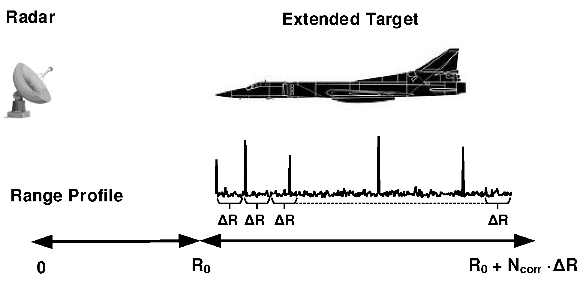
The overall radar system concept is shown in Figure 1. Here it is supposed that the extended target is within [ R 0 , R 0 + N c o r r · Δ R ] , which is partitioned into a set of N c o r r range cells, each one having length equal to Δ R .
The physical interactions between the wave transmitted by the radar and the target can be analyzed by using the so called point scatterer model. According to this model, the received waveform can be evaluated as the sum of time-delayed replicas of the emitted signal, each one weighted with a complex coefficient that represents the response in amplitude and phase of the specific scatterer. In fact, each return is due to one of the target scattering centers. The range cell width will be defined by the waveform resolution which, in turn, depends on the signal bandwidth.
The paper is organized as follows. Section 2 contains the novel contribution, where a series of algebraic manipulations allows to exploit a single pseudo-random bit generator to realize a more complex noise modulation scheme; in this way a noise radar signal can be generated with a very low order of complexity, because it just requires a limited number of memory registers. Section 3 describes the real-time matched filtering; in Section 4 and Section 5 some tests (both by simulation and by an experimental measure) are performed over the proposed algorithm while in Section 6 a comparison is done with other known pulse compression waveforms. Finally, Section 7 reports conclusions and future perspectives.

Notation

This section describes the notation used in the present paper. For what concerns the numerical sets, Z is the set of integers, N is the set of natural numbers, R is the set of real numbers and C is the set of complex numbers. Vectors are denoted by boldface letters, and the symbol ( · ) T stands for transpose. For complex numbers, the symbol ( · ) * stands for conjugate. The symbol · indicates the ceiling function. The notation a , b is used to represent the mathematical interval between a and b, endpoints included, while a , b and a , b exclude the first and the second endpoint respectively. In the digital schematics the item z - 1 corresponds to a discrete time delay equal to the sampling time. As for the signal notation, s ( t ) and s [ n ] stand for continuous-time and discrete-time signals, respectively.

2. Transmitting Section

The properties of the pseudo-random sequences are well known and their use is very common in a wide set of applications (e.g., satellite navigation, telecommunications, cryptography). The have statistical features similar to sequences obtained by random processes but they are generated by deterministic techniques. In fact the generator is modeled by a finite-state machine in which the initial condition is set by a specific key (i.e., the seed); the latter is the only random element while the PN sequence is just the expansion of the seed in a longer string.
With respect to a typical use of the LFSR (e.g., as bipolar modulating signal [14,15,22]), in this work it is exploited in an alternative mode. In fact, noise radar signals are generally synthesized using PN numbers (e.g., [23,24]), so the bit sequences are combined in order to get an approximation of independent uniform random variables.
Let suppose U 0 [ n ] , U 1 [ n ] , ..., U N b i t - 1 [ n ] , as a set of PN bit sequences generated by the same LFSR; the variable n indicates the discrete time. The first step to get good statistical properties is to make them uncorrelated. An immediate way to achieve it consists of cyclic shifts of a single PN sequence, U 0 [ n ] :
U 1 [ n ] = U 0 n - L 1 U N b i t - 1 [ n ] = U 0 n - L N b i t - 1 ,
where L 1 , , L N b i t - 1 Z is a set of arbitrary time shifts.
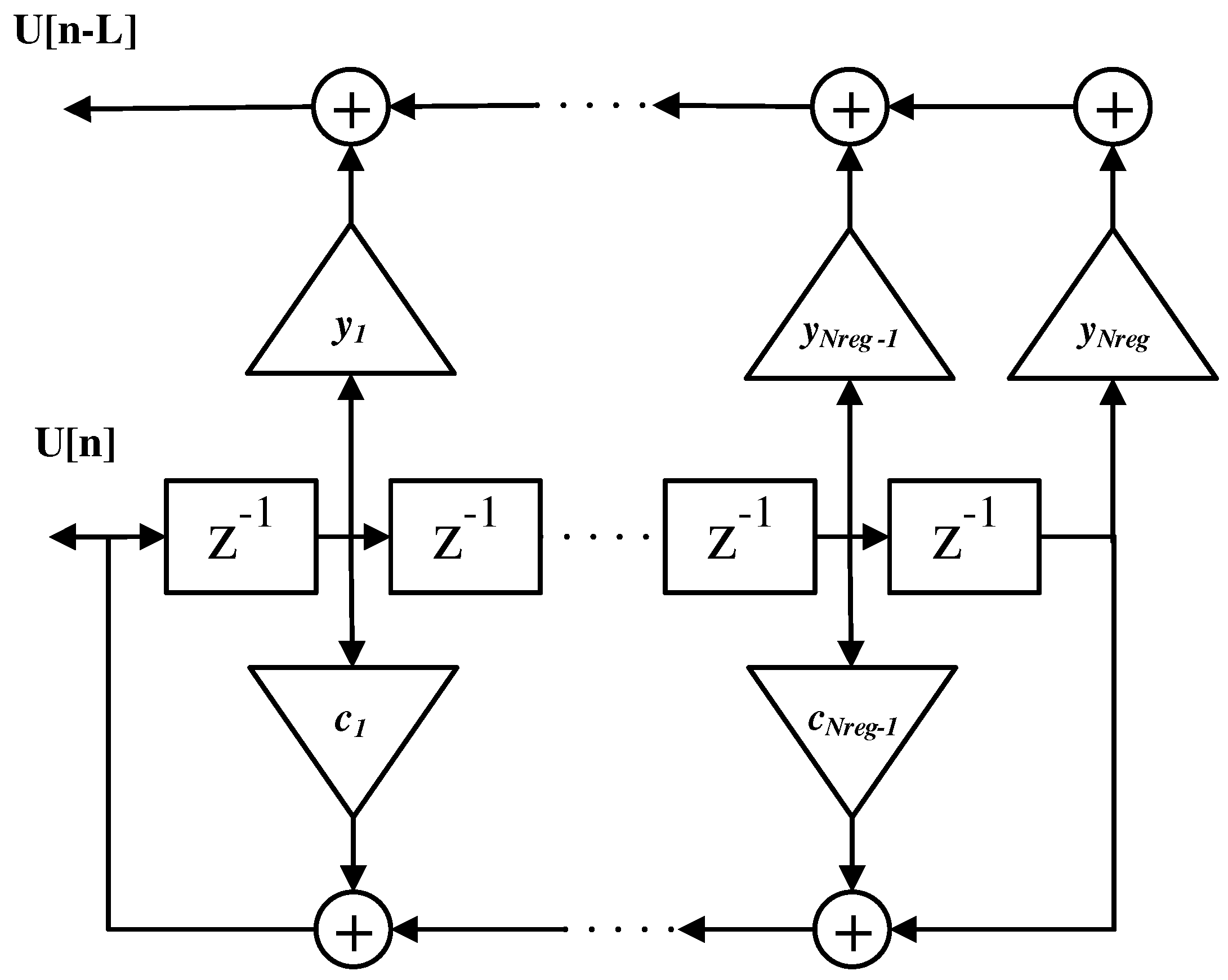
A linear finite-state switching circuit can be modeled by a finite number of adders, memory devices, and constant multipliers connected in any permissible way. In the specific case of the LFSR (see Figure 2), which is a binary switching circuit, the adder is an “exclusive-or” logical block, the memory is represented by an ordinary binary shift register (as the blocks named z - 1 in Figure 2) while the constant multipliers (the terms c 1 , . . . , c N r e g - 1 in Figure 2) for the constant 1 represent connections, and for the constant 0 they are simply no connections. Input and output are assumed to be serial, i.e., they consist of binary data entering an input line one at a time.
In general, it is possible to describe the behavior of this circuit using a polynomial notation [19], as in Equation (2):
h ( x ) = d n - 1 x n - 1 + + d 1 x + d 0 .
Here, the n-th order coefficient is the first term entering the circuit and its effect is the first contribute in output. In this notation a multiplication for x R corresponds to a time shift. Using this notation, the LFSR output can be modeled by a characteristic function, G ( x ) , containing a linear combination of the register binary internal states, U [ n ] :
G ( x ) = n = 0 + U [ n ] x n .
The summation is extended to + because of the feedback in the LFSR (whose schematic is shown in Figure 2).
The term U [ n ] of Equation (3) can be written according to the PN maximal length polynomial:
n = 0 + U [ n ] x n = n = 0 + x n i = 1 N r e g c i U [ n - i ] ,
where
  • N r e g is the number of registers (see Figure 2), also equal to the order of the maximal length polynomial;
  • c i , i = 1 , , N r e g , are the binary polynomial coefficients;
  • U [ n - i ] represents the i-th register content (it can be either 0 or 1).
For each instant, n, the value U [ n ] of the PN sequence corresponds to a linear combination of the N r e g registers:
U [ n ] = c 1 U [ n - 1 ] + + c N r e g U [ n - N r e g ] .
Handling Equation (4) we get:
n = 0 + i = 1 N r e g x n c i U [ n - i ] = n = 0 + i = 1 N r e g x i x n - i c i U [ n - i ] = i = 1 N r e g c i x i n = 0 + x n - i U [ n - i ] .
In the last step of Equation (6) let define the new variable n = n - i :
i = 1 N r e g c i x i n = - i + U n x n = i = 1 N r e g c i x i U [ - i ] x - i + U [ - i + 1 ] x - i + 1 + + + U [ - 1 ] x - 1 + n = 0 + U n x n .
Recalling the definition of G ( x ) , Equation (7) can be written as:
G ( x ) = i = 1 N r e g c i x i U [ - i ] x - i + U [ - 1 ] x - 1 + G ( x ) .
In (8) we can put in evidence G ( x ) :
G ( x ) = i = 1 N r e g c i x i U [ - i ] x - i + U [ - 1 ] x - 1 1 - i = 1 N r e g c i x i .
For the sake of simplicity, the denominator is defined as f ( x ) :
f ( x ) = 1 - i = 1 N r e g c i x i ,
hence Equation (9) becomes:
G ( x ) = i = 1 N r e g c i x i U [ - i ] x - i + U [ - 1 ] x - 1 f ( x ) = i = 1 N r e g l = 1 i c i U [ - l ] x i - l f ( x ) = = i = 1 N r e g c i x i l = 1 i U [ - l ] x - l f ( x ) .
Let introduce a new variable m = i - l . Considering that - l = m - i is the LFSR seed, the condition l = m - i - 1 must be satisfied, which implies i m + 1 . The parameter m, instead, is equal to i - l where max ( l ) = i and i goes from 1 to N r e g so the maximum value that m can assume is N r e g - 1 .
Using the variable m, Equation (11) becomes:
G ( x ) = m = 0 N r e g - 1 x m i = m + 1 n c i U [ - i + m ] f ( x ) = m = 0 N r e g - 1 x m y m + 1 f ( x ) ,
where the coefficients y m can be obtained by the registers content and by the maximal length polynomial coefficients:
y m + 1 = i = m + 1 N r e g c i U [ - i + m ] .
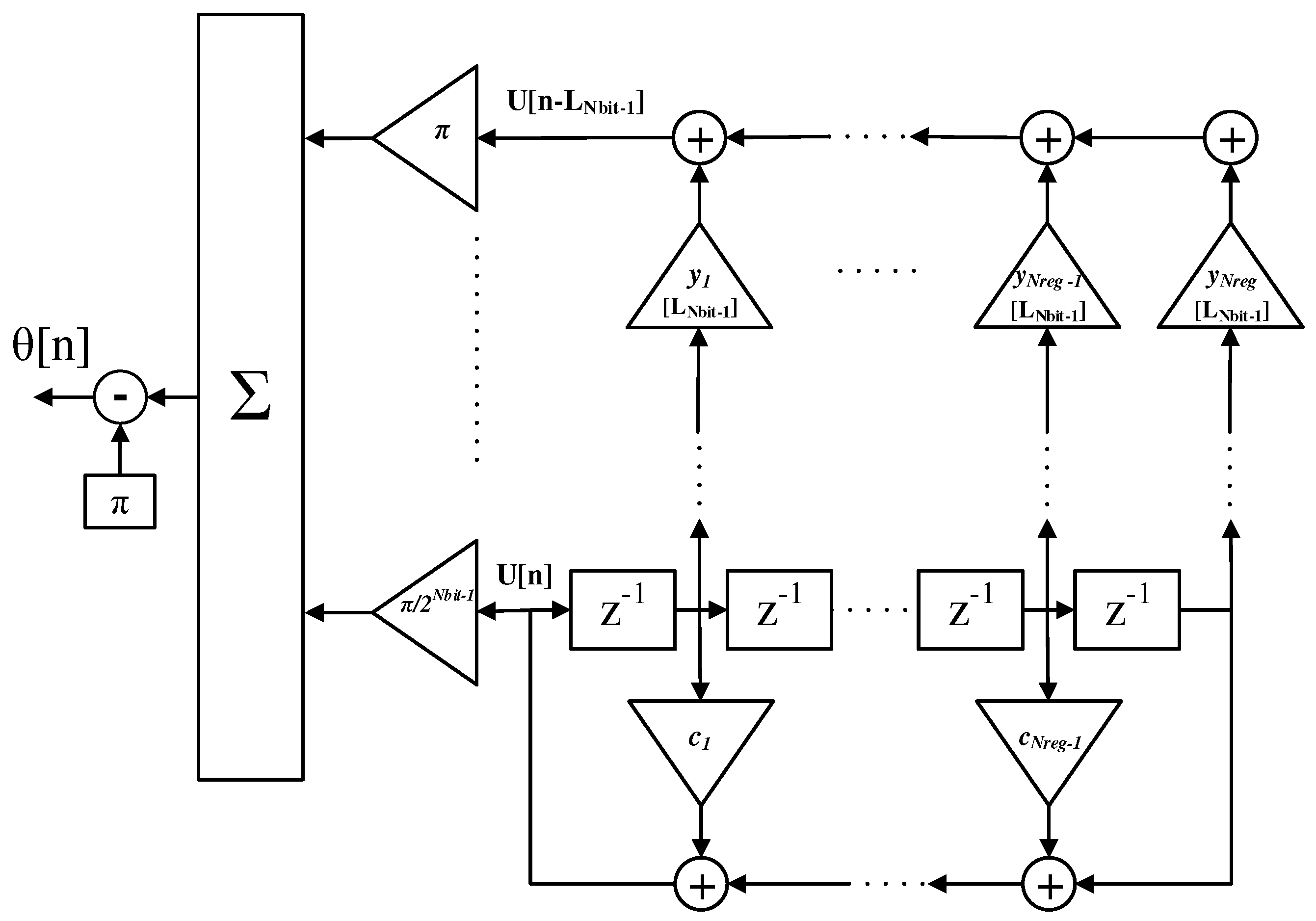
The architecture able to implement this algorithm is shown in Figure 3: here, with a single LFSR generator it is possible to obtain in the same time the PN sequence, U [ n ] , and its delayed replica, U [ n - L ] , by performing a simple combination of the generator registers with the coefficients y 1 [ L ] ,..., y N r e g [ L ] , where L Z is the requested delay.
The last aspect to be investigated consists of the calculation of the appropriate binary coefficients, y 1 [ L ] , ..., y N r e g [ L ] , for the shifted PN sequence U [ n - L ] . We can start by their definition, contained in Equation (13):
y 1 = i = 1 N r e g c i U [ - i ] = c 1 U [ - 1 ] + + c N r e g U [ - N r e g ] y 2 = i = 2 N r e g c i U [ - i + 1 ] = c 2 U [ - 1 ] + + c N r e g U [ - N r e g + 1 ] y N r e g - 1 = i = N r e g - 1 N r e g c i U [ - i + N r e g - 2 ] = c N r e g - 1 U [ - 1 ] + c N r e g U [ - 2 ] y N r e g = i = N r e g N r e g c i U [ - i + N r e g - 1 ] = c N r e g U [ - 1 ] .
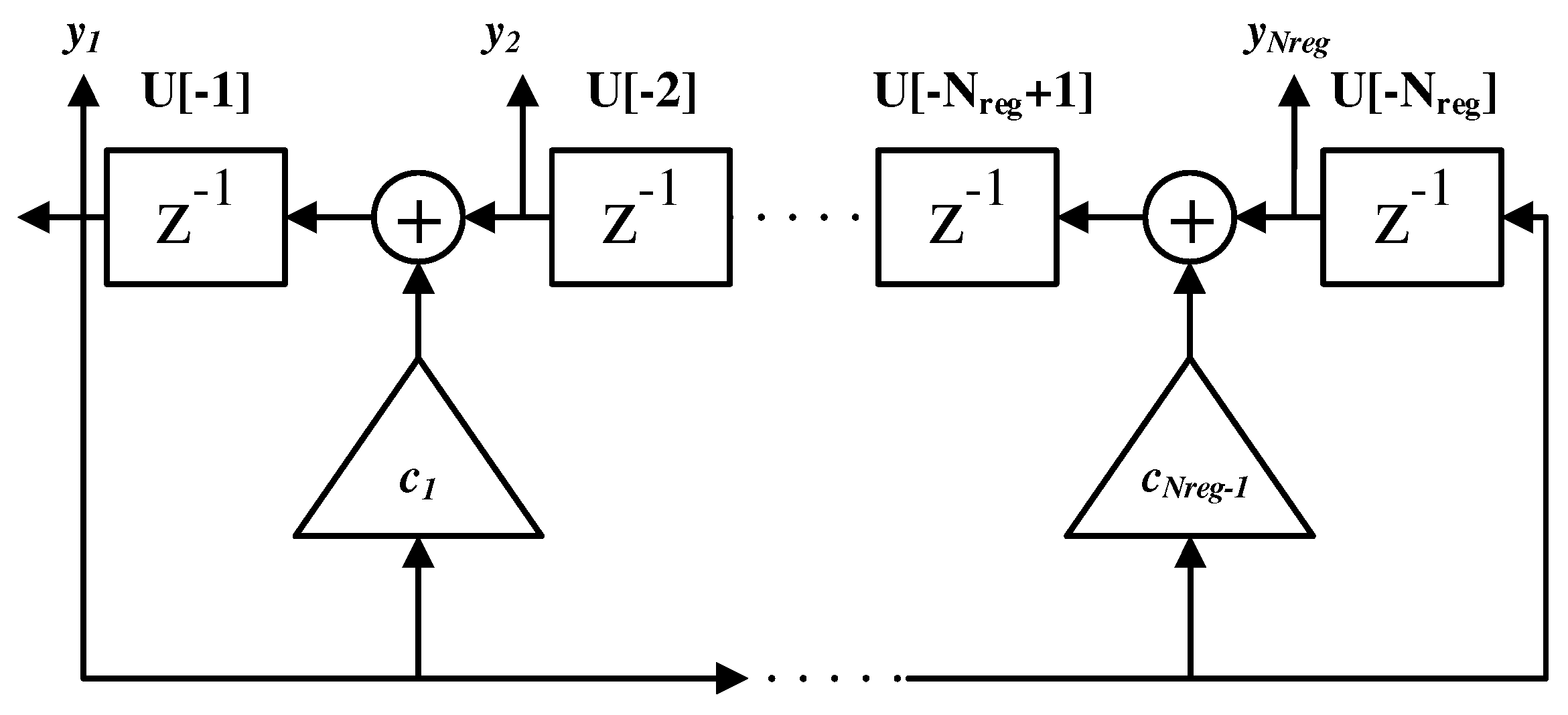
The binary coefficients y 1 , , y N r e g , can be obtained by a further schematic, shown in Figure 4 (which is an alternative way to represent the LFSR, see [19]) and based on Equation (15):
y L [ n ] = i = L N r e g c i y 1 [ n + L - i - 1 ] ,
where c N r e g = 1 and L = 1 , . . . , N r e g .
If the initial conditions are appropriately chosen, the digital structure in Figure 4 is able to generate the same sequence of Equation (14):
y 1 [ 0 ] = U [ - N r e g ] + c N r e g - 1 U [ - N r e g + 1 ] + + c 1 U [ - 1 ] y 2 [ 0 ] = U [ - N r e g + 1 ] + c N r e g - 1 U [ - N r e g + 2 ] + + c 2 U [ - 1 ] y N r e g - 1 [ 0 ] = U [ - 2 ] + c N r e g - 1 U [ - 1 ] y N r e g [ 0 ] = U [ - 1 ] .
In fact (16) is equal to (14) if c N r e g = 1 . This implies:
y 1 [ n ] = U [ n ] ,
where n = 0 , 1 , 2 , . . . , hence the condition
y 1 [ 0 ] = 1 y 2 [ 0 ] = y 3 [ 0 ] = = y N r e g [ 0 ] = 0
coincides with
U [ - N r e g ] = 1 U [ - N r e g + 1 ] = = U [ - 2 ] = U [ - 1 ] = 0 .
At the L-th step, the registers of the generator in Figure 4 contain the appropriate coefficients y n needed to generate the initial sequence delayed of L steps, i.e., U [ n - L ] . This algorithm can be generalized on r delays by overlapping r similar structures; in this way we are able to obtain U [ n ] , U [ n - L 1 ] , , U [ n - L r ] .
The approximation of the uniform random number in [ - π , + π ) is then obtained by combining a set of N b i t PN sequences as follows:
θ [ n ] = π U N b i t - 1 [ n ] + + π 2 N b i t - 2 U 1 [ n ] + π 2 N b i t - 1 U 0 [ n ] - π ,
where
U 1 n = U 0 n - L 1 U N b i t - 1 n = U 0 n - L N b i t - 1 .
The overall phase generation schematic, including all the theory mentioned above, is shown in Figure 5. The generated waveform, s ( t ) , consists of a phase modulated signal (without loss of generality, in the presented development, we deal with the baseband signal; the corresponding radio-frequency (RF) signal, on a carrier f c , would be equal to s R F ( t ) = 2 · R e e j 2 π f c t · s ( t ) , where R e {} is the real part of a complex number):
s ( t ) = e j ϕ ( t ) ,
where
ϕ ( t ) = n = - + θ [ n ] r e c t t - n T c T c .
Equation (23) represents a sequence of pseudo-random phase symbols with duration T c . The variable θ [ n ] - π , + π , obtained using (20), can result as a good approximation of a uniform random variable if the appropriate values of N b i t and N R e g are chosen.
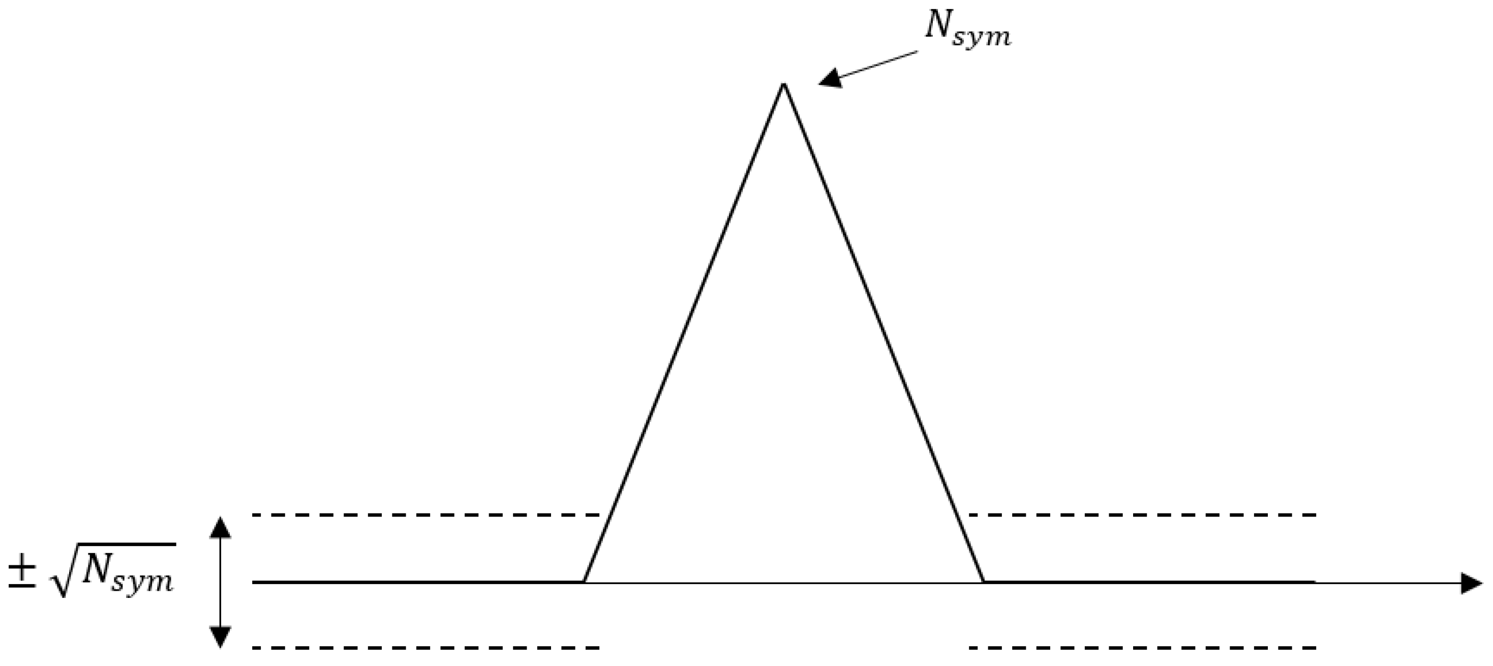
It can be proved (proofs are shown in Appendix A) that under this condition the auto-correlation function (ACF) of s ( t ) has a triangular shape with base equal to 2 T c and a peak to side-lobe ratio (PSLR) equal to:
P S L R = 10 · l o g 10 B T 10 · l o g 10 N s y m ,
with N s y m representing the number of integrated phase symbols and B T the time-bandwidth product.
The LFSR generator can be initialized using a specific seed such that the same sequence, appropriately shifted according to the target position, can be locally generated in reception, realizing a sub-optimal matched filter.
The shift is easily performed by using the LFSR seed related to that specific delay. In fact, when the initial seed is known (e.g., in the presence of a designation, as in [18]), the “maximal length” code is a deterministic sequence: it can be written in a look-up table (LUT) of the same form of Table 1. Each seed (i.e., the digital word, [ b N r e g - 1 , , b 0 ] , that sets the generator state) corresponds to a specific delayed signal replica.
This architecture results as a powerful solution for some hardware constraints [18]: in fact it theoretically permits an unlimited integration because samples of the reference signal do not have to be stored.
In the remainder of this paper the exploited sequence, called PN22, is generated using the values of Table 2. Its total length, M = 2 22 - 1 , is suitable for the storage of the PN22 in a LUT similar to Table 1, showing, in the same time, good statistical properties.

3. Receiving Section

Performing real time matched filtering in noise radar technology (NRT) is a challenging task [25]. Once the baseband signal components have been obtained, matched filtering can be performed by evaluating a real time cross-correlation (i.e., using the multichannel correlator [16,17,18], whose digital schematic is shown in Figure 6): exploiting the LFSR generator programmability an appropriately shifted local replica is generated by setting a specific initial seed.
In the correlation block the received signal, s I n , is coherently detected and multiplied to N c o r r delayed and conjugated local replicas ( s R e f * ). The output of this operation consists of a set of N c o r r complex values, r 0 , , r N c o r r - 1 T c C , each one representing a single cross-correlation bin dumped after the integration time, T.
The sums are done over a fixed number N s y m of phase symbols and this procedure is equivalent to a coherent integration, because it takes into account both the amplitude and the phase information: moreover, the integration time T can be expressed according to N s y m , using the signal sampling time, T s , and the cross-correlation sampling step, equal to the chip time T c , as in Equation (25):
T = N s y m · T c T s · T s .
A set of N c o r r accumulation block is needed in order to obtain the cross-correlation on the desired domain. Nowadays a modern field programmable gate array (FPGA) is able to handle a few thousands of these simple units, so implementing such algorithm on a real time board does not represent a critical problem.
The resulting profile can be expressed in vector notation, as follows:
r = r 0 , , r k , , r N c o r r - 1 T c T ,
in which the generic k-th bin can be written in explicit form:
r k = n = 1 N s y m · T c T s s i n n T s · s R e f * n T s - k T c .
The main parameters of Equation (27) are:
  • k, the index of the range bin;
  • N s y m N , the number of integrated PN phase symbols;
  • s i n [ n T s ] , the digital complex envelope of the received signal;
  • T s , the sampling time;
  • T c , the symbol duration;
  • s R e f * n T s - k T c , the conjugated local replica of the transmitted signal, delayed of k range cells.
The architecture proposed in this Section, compared to the typical noise radar ones, permits a reduction in terms of hardware complexity, especially for long term integration processes.
Let us consider, for example, the case described in [18]: here, with an integration time of 80 ms and a sampling time equal to 0.5 ns, it would be required a matched filter or a fast Fourier transform (FFT) with 160 × 10 6 coefficients while using the proposed approach only a set of N c o r r calculus units is needed (order of some hundreds, depending on the range profile length).
Moreover, in the latter case, the integration time is limited by the number of bits used in the digital integrator of the FPGA-based correlator.
The main issue in this architecture is given by scatterers showing time misalignments of a fraction of the sampling interval respect to the reference values used in the correlator. This problem could be overcome by decreasing the time distances between consecutive range cells, i.e., by generating a reference signal equal to s R e f * n T s - k T c γ , where γ N and γ > 1 . Given the same range profile length, this procedure increases the number of range cells needed in the correlator but, in general, the hardware complexity still remains lower than a typical matched filter.
In the remainder of this paper the receiving section is dimensioned according to the parameters of Table 3 (theoretically, in presence of a couple of scatterers and considering the ACF triangular shape described in Appendix A, we would be able to distinguish the two different correlation peaks if the latter show a relative delay of at least one chip, hence we considered a resolution equal to T c ; the selected value for the chip duration, T c , gives a range resolution which is roughly one order of magnitude lower than the HRRP definitions suggested by some authors, e.g. [26], hence the value of 40 ns was actually chosen according to the equipment at our disposal for the laboratory tests of Section 5 but, in any case, better performances in terms of range resolution can be achieved with a larger bandwidth).

4. Simulations

The algorithm described in the previous Sections has been modeled in Simulink and the baseband noisy waveform was simulated in two different configurations to evaluate its features in terms of average PSLR and resolution. These two performances have been evaluated over a window of 400 range bins. The following two scenarios have been chosen in order to be emulated also using real equipment, as mentioned in Section 5.
The resulting range profiles are obtained by evaluating the absolute value of the multichannel correlator output.

4.1. Test on PSLR

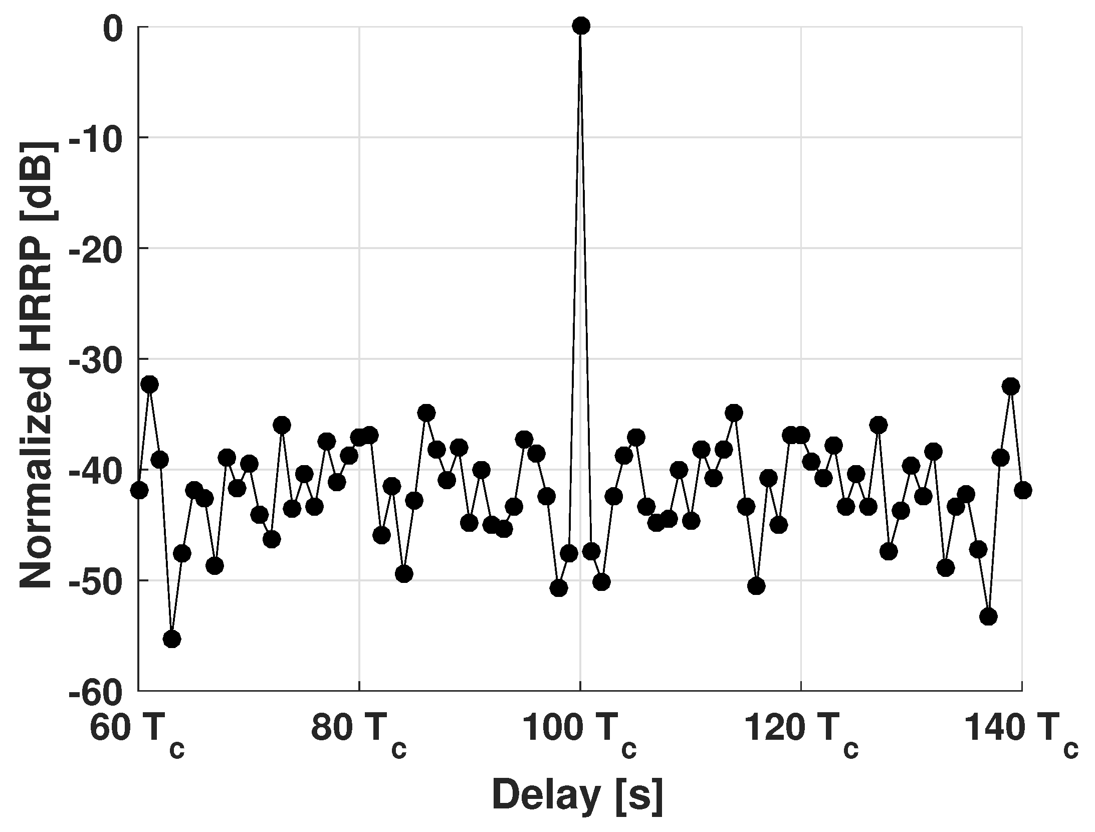
In the first test, a single scatterer placed at bin #100 of the range window has been simulated. The integration, performed by a Simulink model of the multichannel correlator, was done over N s y m = 10 4 phase symbols. The result is shown in Figure 7.
The average PSLR is coherent to the theoretical evaluation of Equation (24): in fact, considering N s y m = 10 4 the expected PSLR is equal to 40 dB.

4.2. Test on Resolution

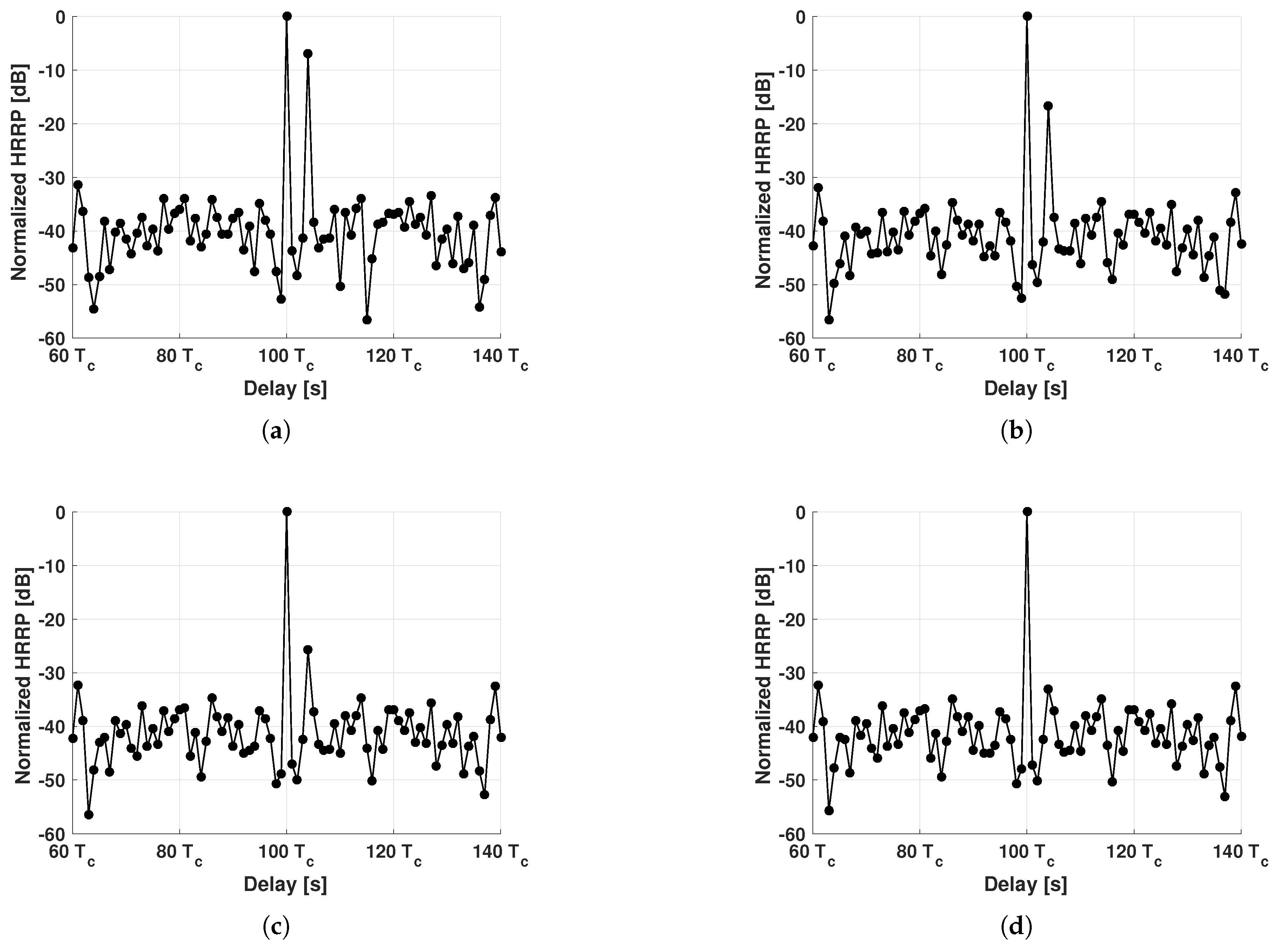
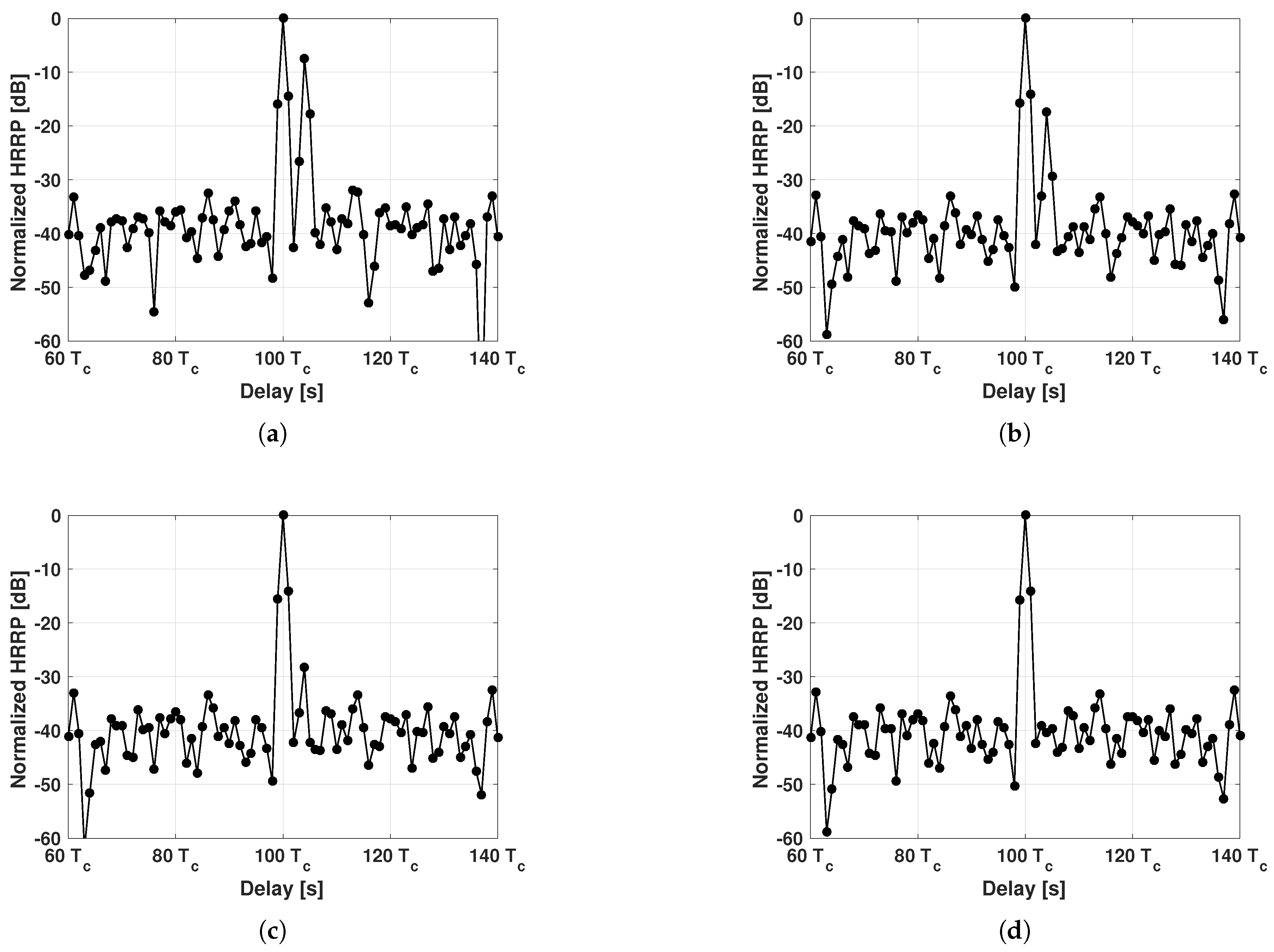
In this test a second scatterer was simulated as well as the scatterer placed at bin #100: it was supposed to be at bin #104 and to have different attenuations with respect to the main one: 7, 17, 27 and 37 dB. The results are shown in Figure 8.
They show good performances both in terms of PSLR and in terms of range resolution. In fact the secondary scatterer is recognizable until its relative attenuation with respect to the main peak is greater than the average side-lobe level (equal to −40 dB).

5. Experimental Measures

According to the situations already described in Section 4.1 and Section 4.2, the proof of concept has been performed in laboratory, in order to test the proposed algorithm on real equipment.
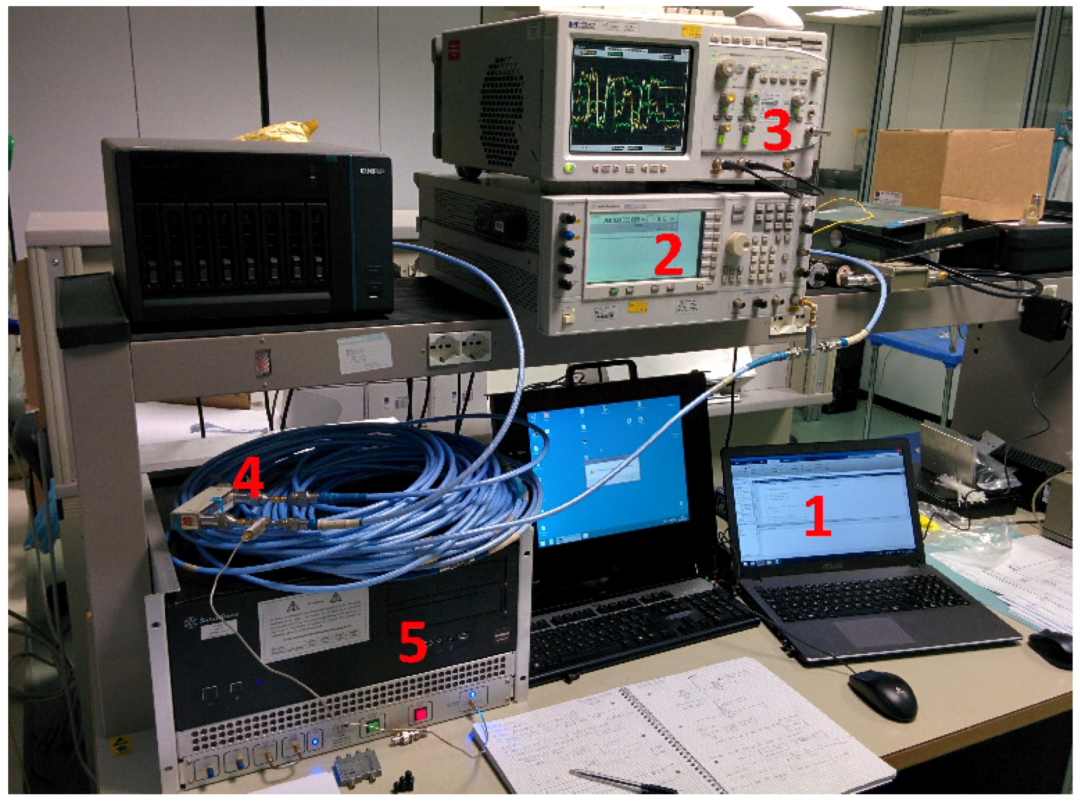
The pseudo-noise phase sequence, PN22, with N s y m = 10 4 , was generated in an offline mode using Simulink and then downloaded to an Agilent E8267C [27] signal generator by a GPIB-USB connection [28]. Among the functions of the RF generator, there was the possibility to perform I/Q modulations starting from arbitrary phase sequences. In our case, as already described in the previous sections, the PN22 phase samples were defined using 4 bits, hence a 16-PSK modulation was performed. The latter transmitted the resulting RF signal with a bandwidth (BW) of 100 MHz (maximum bandwidth allowed by the signal generator hardware) and with a chip width, T c , equal to 40 ns. The specific value of the chip duration was defined in order to optimize the available bandwidth.
As in Section 4, the resulting range profiles are obtained by evaluating the absolute value of the multichannel correlator output.

5.1. Test on PSLR

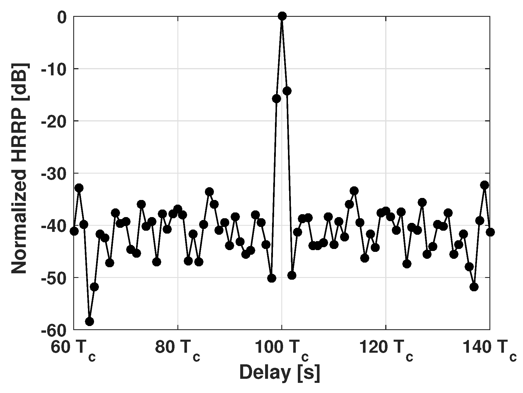
To evaluate the performance in terms of PSLR, the signal was modulated on a carrier of 700 MHz (the carrier frequency was selected according to the available sampler) and transmitted on a short RF cable [29], necessary to emulate the signal propagation. The resulting signal was then sampled at 2.2 GHz and recorded on a solid state hard disk which allowed an offline processing in Simulink: the model we used was the same of Section 4. Starting from the recorded sampled signal (received on the carrier of 700 MHz), a demodulation was done and the samples of the digital complex envelope were processed using the model of Figure 6. The local reference signal was generated with an appropriate offset in order to place the correlation peak on bin #100, as in the simulations. The schematic of the set-up is shown in Figure 9 while the amplitude of the resulting cross-correlation is shown in Figure 10.
With respect to the same test done via simulation (see Figure 7), we got a similar PSLR but a degraded resolution. In fact the level of the samples adjacent to the peak is very high: this effect is due to the limited bandwidth of the RF generator.

5.2. Test on Resolution

In this case the modulated signal, already cited in Section 5.1, was divided and transmitted through two different paths, i.e., a short cable (the direct path) and a 43 m folded RF cable [29] connected to a variable microwave attenuator [30] (see Figure 11 and Figure 12) . This latter was used to emulate a secondary scatterer A dB below the direct path, delayed of 4 T c with respect to the latter. The two signals after being summed were sampled, recorded and processed in the same manner of Section 5.1.
The resulting profiles are shown in Figure 13: the main scatterer (direct path) is centered on bin #100 (the same delay of Section 5.1 was exploited in order to get the correlation peak on bin #100 of the range window). The first three values of the attenuation A exploited during the tests (i.e., 7, 17 and 27) are correctly represented by the normalized resulting profiles while the last one (i.e., 37 dB) is not recognizable because of the correlation sidelobes. The average PSLR is coherent with the theoretical value of 40 dB ( N s y m = 10 4 ). The correlation triangular shape was spread on the adjacent bins due to the limited transmitter BW.

6. Discussion

As already stated in the previous Sections, to obtain high resolution range profiles, waveforms with narrow peak of the ACF and low time sidelobes are typically needed [31]. In technical literature several items ensuring these two properties can be found [32,33,34,35]. They basically tend to achieve a narrow ACF peak by keeping the PSLR as low as possible. In this context, a comparison of the waveform proposed by this paper (i.e., PN22) with respect to other ones can be done. Using a simulation approach, five terms of comparison are taken into account:
  • pure unimodular noise;
  • linear chirp;
  • non linear frequency modulation (NLFM) signal;
  • hybrid non linear frequency modulation (HNLFM) signal;
  • Barker code with 13 symbols;
  • Frank code with 16 2 = 256 phase symbols.
Once the BW is set, the direct consequence is a fixed resolution. To guarantee a fair comparison, all the waveforms were defined on the same − 3dB BW, 35 MHz, and on the same integration time, T = 50 μ s (i.e., an equal compression ratio, B T ).
In the pure unimodular noise waveform, based on the model of [24,34], the I and Q samples were obtained through a white Gaussian random process and the resulting signal was filtered using a rectangular-shaped filter. The linear chirp, the NLFM and the HNLFM waveforms were simulated using the same compression ratio; in particular, the second and the third ones, were created using the parameters found in [33]. The difference between the NLFM and the HNLFM is that the latter also shows a specific amplitude modulation.
The last two codes, i.e., Barker and Frank, were generated considering the same chip width of the PN sequence proposed in Section 2; in this way the constraint related to the BW was respected.
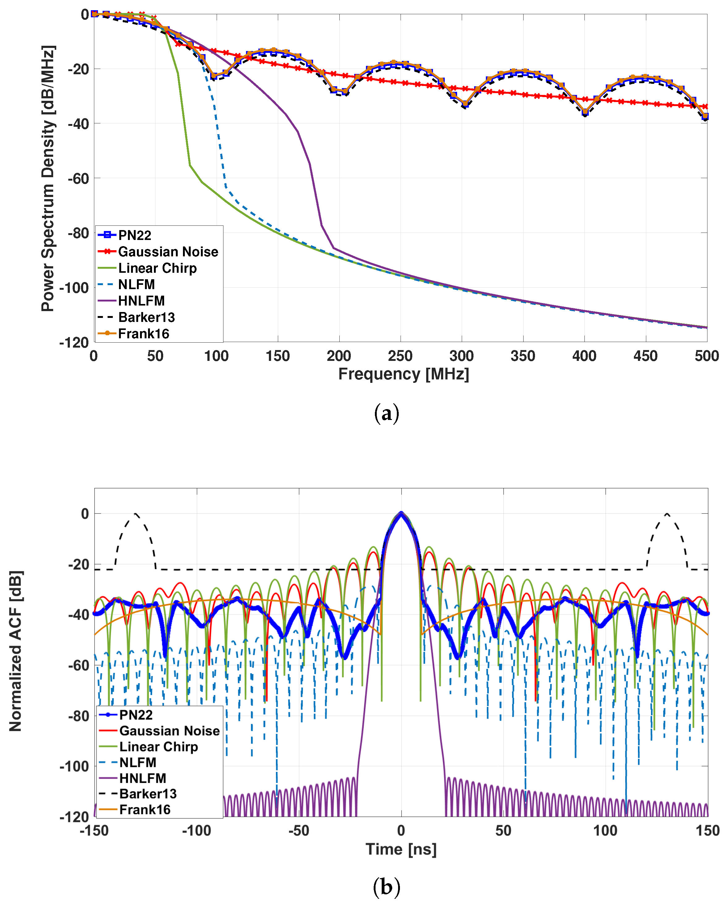
The power spectrum density (PSD) and the ACF of the tested sequences are shown in Figure 14. The pure unimodular noise waveform and the chirp signal, having similar PSDs, show the same behavior in terms of resolution (intended as the main lobe width) equal to T c = 10 ns and of PSLR, 15 dB for the first and 13 dB for the second (the difference is given by the non-perfect rectangular shape of the low-pass filtering). With respect to the PN22 sequence, the chirp signal has a limited duration (equal to T) while the noise-like waveform would require a more complex digital generation scheme.
The NLFM shows improved performances in terms of PSLR with respect to the linear case (29 dB compared to 13 dB obtained with the linear chirp).
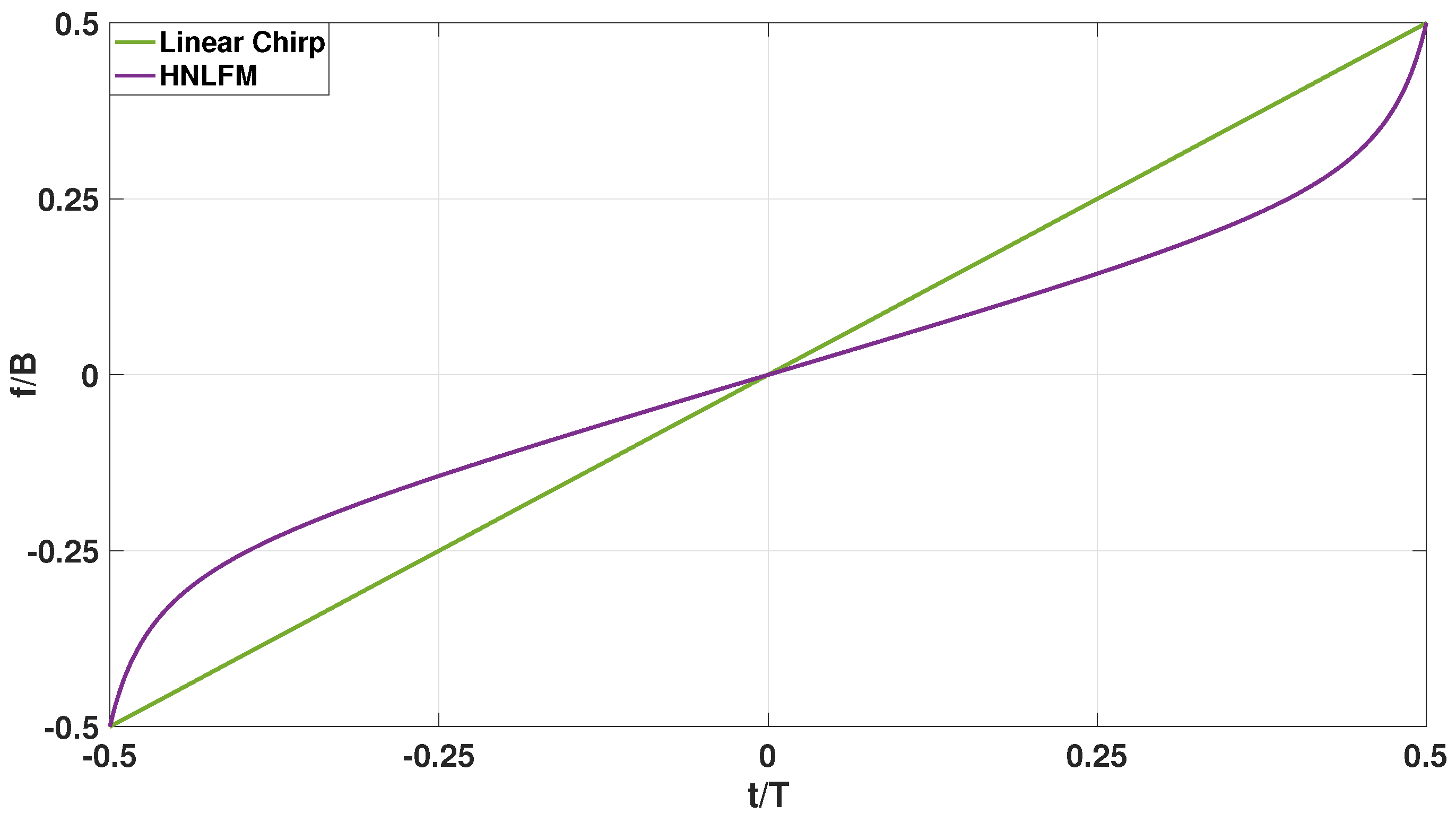
For what concerns the HNLFM waveform a good PSLR value was got (i.e., 104 dB with respect to PN22, where it is equal to 34 dB) but a higher complexity is needed in the signal generation phase: in fact an amplitude modulation is required and it causes a loss of efficiency in the transmitter. Given the deterministic nature of the HNLFM it is easier to intercept it with respect to a noisy waveform. Furthermore, the period of this code is limited to the integration time T; in fact, both for the linear and for the non linear chirps, the modulating sequence will repeat every T seconds (see Figure 15) and this causes an ambiguity in range.
In terms of resolution, the Barker 13 sequence has the same behavior of the PN22 but limited performances if we consider the code period (only 13 symbols) and the PSLR (22.3 dB).
Similar issues are present in the last comparison between the PN22 and the Frank code: this latter was generated with a phase quantum of 22 . 5 corresponding to 4 bits of quantization (256 total symbols). This constraint was imposed in order to be coherent with the PN22 generation (quantized using 4 bits). These two signals have similar performances both in terms of resolution and of PSLR but the Frank code is limited by the repetition period, equal to N 2 = 256 chips.
In general, a disadvantage of pseudo-random signals with respect to deterministic ones resides in the optimization of the single waveform: in fact, in NRT field, we define a “family” of signals rather than the specific waveform.
Table 4 summarizes the advantages/disadvantages of each of the tested waveforms in terms of main lobe width, PSLR, repetition period and complexity in the generation phase.
7. Conclusions

The design of the transmitted waveform represents a key factor for the generation of radar HRRPs. In fact, it affects the most important parameters of a range profile, i.e., the resolution and the side-lobe level, both related to the capability to distinguish different scatterers of extended targets.
In this paper a pseudo-random radar waveform and a related processing scheme were proposed: the design was focused on a real time approach, capable of handling long time integrations with a computational burden as low as possible. The LFSR based generator permits the realization of a sub-optimal low complexity matched filter in reception. Due to the absence of a reference signal storage, the integration process can be theoretically unlimited: it results as a fundamental aspect to get suitable performances also in low ERP conditions. Therefore, the proposed algorithm can be fully exploited on bistatic/monostatic architectures with strict requirements in terms of ERP and/or processing resources. A typical noise radar processing chain, for example, would require to store the transmitted samples as reference: this represents an important issue for long time integrations hence the proposed architecture can provide a possible solution.
The mathematical model of the signal generator and the multichannel correlator were discussed and evaluated. The “proof of concept” was validated using both a simulation approach and a laboratory experiment: in these phases, the high robustness and versatility of the architecture was proved in terms of resolution and sidelobe level. A comparison to other known pulse compression waveforms was also done and the main differences were shown.

Acknowledgments

The authors wish to thank Gaspare Galati for stimulating and addressing this work, Danilo Orlando for his helpful reviews and suggestions and their colleagues Luca Arena, Federico D’Abbieri and Roberto Starna for the help provided during the measurement campaign. Part of the present work was funded by an internal research program of Elettronica SpA.

Author Contributions

Davide Massaro contribution includes: algorithm implementation, tests preparation and relative analysis as well as paper writing. Riccardo Ardoino proposed the basic ideas and gave the theoretical support while Marco Grazzini defined the pseudo-noise phase sequence generation algorithm.

Conflicts of Interest

The authors declare no conflict of interest.

Appendix A. Analytical Considerations about the ACF of the Designed Waveform

Appendix A.1. ACF Shape

The waveform exploited in this work consists of a phase modulated signal having the form of Equation (22).
To correctly design the LFSR based generator of Figure 5, ACF of s ( t ) has been first assessed from a theoretical point of view, exploiting its probabilistic/statistical definition [36]:
R s ( τ ) = E s ( t ) · s * ( t + τ ) = E e j ϕ ( t ) · e - j ϕ ( t + τ ) = E e j ϕ ( t ) - ϕ ( t + τ ) .
Let define the new variable θ ( τ ) as
θ ( τ ) = ϕ ( t ) - ϕ ( t + τ ) ,
hence Equation (A1) can be written as
R s ( τ ) = E e j θ ( τ ) = Θ e j θ ( τ ) · f θ ( θ ; τ ) d θ .
In Equation (A3) the term f θ ( θ ; τ ) represents the probability density function (PDF) of the variable θ ( τ ) and it can be evaluated starting from Equation (23) and supposing the coefficients θ [ n ] as statistically independent random variables with a uniform PDF in [ - π , + π ) .
Under these conditions, we can evaluate two different cases:
(I) 0 | τ | T c
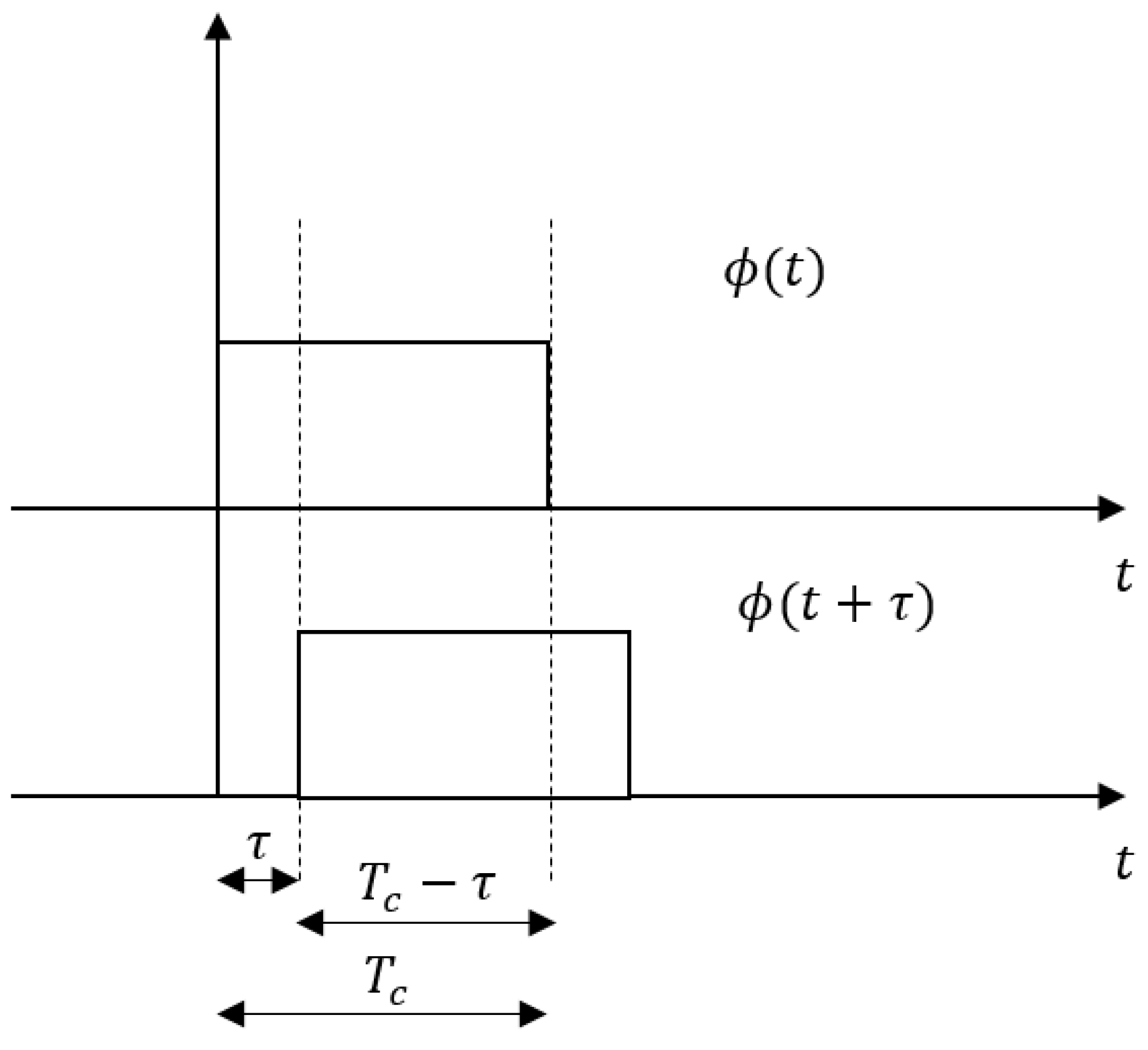
In this case the samples of s ( t ) show a partial overlap, as can be seen in Figure A1.
Figure A1. Representation of the two components of θ ( τ ) , i.e., ϕ ( t ) and ϕ ( t + τ ) , with respect to the time shift, τ .
Aerospace 05 00004 g0a1
With a probability equal to τ T c , ϕ ( t ) and ϕ ( t + τ ) can be assumed as two different random variables while they corresponds to the same value with a probability of T c - | τ | T c .
(II) | τ | > T c
In this other case, there is no overlap between the variables ϕ ( t ) and ϕ ( t + τ ) , hence they can be considered as two independent and identically distributed random variables with uniform PDF.
By combining what found in the items I and II, the PDF of the variable θ can be written in explicit form:
f θ ( θ ; τ ) = δ ( θ ) · T c - | τ | T c + 1 2 π · r e c t θ 2 π · | τ | T c , f o r | τ | T c 1 2 π · r e c t θ 2 π , f o r | τ | > T c .
Substituting the analytical expression of f θ ( θ ; τ ) in Equation (A3) we get:
R s ( τ ) = 1 - | τ | T c , f o r | τ | T c 0 , f o r | τ | > T c .
Equation (A5) demonstrates that the theoretical ACF of s ( t ) has a triangular shape with a unitary peak and the base equal to 2 T c .

Appendix A.2. PSLR Evaluation

The PSLR can be easily evaluated by considering the ACF statistics of the proposed signal (see Section 2) at the output of the multichannel correlator (described in Section 3). The main statistical information are:
  • the expected value of the output (k-th bin):
    E r k = E n = 1 N s y m · T c T s s i n n T s · s R e f * n T s - k T c ,
  • the second non central moment of the output (k-th bin):
    E r k 2 = E n = 1 N s y m · T c T s s i n n T s · s R e f * n T s - k T c 2 ,
  • and finally the root mean square (RMS) value of the output (k-th bin):
    σ r k = E r k 2 - E r k 2 .
The expected value provides information about the “averaged behavior” whereas the RMS indicates some displacement with respect to the former. In particular the sidelobes evaluated in this phase should be intended as the RMS expected value outside the chip time T c .
To evaluate the ACF, we can suppose s R e f * n T s - k T c = s i n * n T s - k T c , and T c = T s (one sample per chip).
We can calculate Equations (A6)–(A8) on the peak ( k = 0 , i.e., when the input sequences are perfectly overlapped) and on the sidelobes ( k 0 , i.e., when the chips are not correlated).
In the first case ( k = 0 ) we get:
E r 0 = E n = 1 N s y m s i n n T s · s I n * n T s = N s y m .
E r 0 2 = E n = 1 N s y m s i n n T s · s I n * n T s 2 = N s y m 2 .
σ r 0 = E r 0 2 - E r 0 2 = 0 .
In the second case ( k 0 ) we get:
E r k = E n = 1 N s y m s i n n T s · s i n * ( n - k ) T s = 0 .
E r k 2 = E n = 1 N s y m s i n n T s · s i n * ( n - k ) T s 2 = N s y m .
σ r k = E r k 2 - E r k 2 = N s y m .
These results are then exploited to evaluate the PSLR in dB, as done in Equation (24) (see also Figure A2)
P S L R = 20 · l o g 10 N s y m N s y m = 10 · l o g 10 ( N s y m )
Thanks to this evaluation it has been proved that the “statistical behavior” of the ACF is such that the PSLR (on a linear scale) increases as a linear function of N s y m (i.e., number of integrated independent phase symbols).
However, this is just a statistical indication used in dimensioning the LFSR length: in fact it can happen that the specific realization of a sequence can show higher sidelobes with respect to the RMS value (an example is shown in Figure A3).
Figure A2. Triangular shape of the ACF and relative level of the RMS sidelobes level.
Aerospace 05 00004 g0a2
Figure A3. Example of an ACF evaluated over a limited number of samples: here, as happens on real cases, some sidelobes might overcome the RMS level.
Aerospace 05 00004 g0a3
The bandwidth B of Equation (24) is considered as the 3 dB-bandwidth of the rectangular pulse:
B 1 / T c
Under this condition, by exploiting an integration over a time interval T, the product B T becomes:
B T 1 T c · T = T T c = N s y m
An this justifies also the first member of Equation (24).

References

  1. Peterson, P.; Weldon, E.J. Introduction to Radar Target Recognition; n. 18 in Radar, Sonar and Navigation Series; The Institution of Engineering and Technology (IET): London, UK, 2006; ISBN 9780863415012. [Google Scholar]
  2. Blacknell, D.; Griffiths, H. Radar Automatic Target Recognition (ATR) and Non-Cooperative Target Recognition (NCTR); n. 33 in Radar, Sonar and Navigation Series; The Istitution of Enginenering and Technology (IET): London, UK, 2013; ISBN 9781849196857. [Google Scholar]
  3. Wasselin, J.P.; Mazuel, S.; Itcia, E.; Hizing, A.; Theil, A. FMCW radar system for detection and classification of small vessels in high sea state conditions. In Proceedings of the 42nd European Microwave Conference, Amsterdam, The Netherlands, 29 October–1 November 2012; pp. 29–32. [Google Scholar]
  4. Jasinski, T.; Antipov, I.; Monteiro, S.T.; Brooker, G. W-band maritime target classification using high resolution range profile. In Proceedings of the International Conference on Radar, Adelaide, Australia, 9–12 September 2013; pp. 356–361. [Google Scholar]
  5. Borrion, H. Study of Processing Techniques for Radar Non-Cooperative Target Recognition. Ph.D. Thesis, University of London, London, UK, 2006. [Google Scholar]
  6. Li, H.J.; Yang, S.H. Using range profiles as feature vectors to identify aerospace objects. IEEE Trans. Antennas Propag. 1993, 41, 261–268. [Google Scholar] [CrossRef]
  7. Zyweck, A.; Bogner, R.E. Radar target classification of commercial aircraft. IEEE Trans. Aerosp. Electron. Syst. 1996, 32, 598–606. [Google Scholar] [CrossRef]
  8. Levanon, N.; Mozeson, E. Radar Signals; John Wiley & Sons: Hoboken, NJ, USA, 2004; ISBN 9780471663072. [Google Scholar]
  9. Skolnik, M.I. Introduction to Radar Systems, 3rd ed.; McGraw-Hill: New York, NY, USA, 2001; ISBN 9780072881387. [Google Scholar]
  10. Lukin, K. Dedicated applications of noise radars. In Proceedings of the 16th International Radar Symposium, Dresden, Germany, 24–26 June 2015; pp. 771–776. [Google Scholar]
  11. Axelsson, S.R.J. Noise radar using random phase and frequency modulation. IEEE Trans. Geosci. Remote Sens. 2004, 42, 2370–2384. [Google Scholar] [CrossRef]
  12. Galati, G.; Pavan, G.; De Palo, F.; Stove, A. Potential applications of noise radar technology and related waveform diversity. In Proceedings of the 17th International Radar Symposium, Krakow, Poland, 10–12 May 2016; pp. 1–5. [Google Scholar]
  13. Yue, W.; Li, L.; Yu, X.; Tao, H. Radar constant-modulus waveform optimization for high-resolution range profiling of stationary targets. Sensors 2017, 17, 2574. [Google Scholar] [CrossRef] [PubMed]
  14. Lukin, S.; Zemlyaniy, O.; Lukin, K. FPGA based random waveform generators for noise radars. In Proceedings of the 16th International Radar Symposium, Dresden, Germany, 24–26 June 2015; Volume 2, pp. 777–782. [Google Scholar]
  15. Lukin, S.; Zemlyaniy, O.; Lukin, K. FPGA-based devices for random waveform generation and stepped delay signal processing. In Proceedings of the Signal Processing Symposium, Debe, Poland, 10–12 June 2015; pp. 1–7. [Google Scholar]
  16. Vyplavin, P.; Melnikova, E.; Lukin, S. Real-time signal processing in noise radar. In Proceedings of the 11th International Radar Symposium, Vilnius, Lithuania, 16–18 June 2010; pp. 1–3. [Google Scholar]
  17. Lukin, K.A.; Zemlyaniy, O.V.; Tatyanko, D.N.; Lukin, S.; Pascazio, V. FPGA-based time-integrating multichannel correlator for noise radar applications. In Proceedings of the 9th International Kharkiv Symposium on Physics and Engineering of Microwaves, Millimeter and Submillimeter Waves, Kharkiv, Ukraine, 20–24 June 2016; pp. 1–5. [Google Scholar]
  18. Massaro, D.; Ardoino, R. Range profiling of vessels with pseudo-random radar waveforms. In Proceedings of the IEEE First Ukraine Conference on Electrical and Computer Engineering, Kiev, Ukraine, 29 May–2 June 2017; pp. 243–248. [Google Scholar]
  19. Peterson, W.W.; Weldon, E.J. Error-Correcting Codes, 2nd ed.; MIT Press: Cambridge, MA, USA, 1972; ISBN 9780262160391. [Google Scholar]
  20. Thomas, D.B.; Luk, W. The LUT-SR family of uniform random number generators for FPGA architectures. IEEE Trans. Very Large Scale Integr. (VLSI) Syst. 2013, 21, 761–770. [Google Scholar] [CrossRef]
  21. Alves, J.D.; Evans, G.E. Digital pseudorandom uniform noise generators for ADC histogram test. In Proceedings of the Conference on Design of Circuits and Integrated Systems, Estoril, Portugal, 25–27 November 2015; pp. 1–6. [Google Scholar]
  22. Albanese, D.F.; Klein, A.M. Pseudorandom code waveform design for CW radar. IEEE Trans. Aerosp. Electron. Syst. 1979, 15, 67–75. [Google Scholar] [CrossRef]
  23. Galati, G.; Pavan, G.; De Palo, F. Noise radar technology: Pseudorandom waveforms and their information rate. In Proceedings of the 15th International Radar Symposium, Gdansk, Poland, 16–18 June 2014; pp. 123–128. [Google Scholar]
  24. Galati, G.; Pavan, G.; De Palo, F. Generation of pseudo-random sequences for noise radar applications. In Proceedings of the 15th International Radar Symposium, Gdansk, Poland, 16–18 June 2014; pp. 115–118. [Google Scholar]
  25. Savci, K.; Erdogan, A.Y.; Gulum, T.O. Software defined L-band noise radar demonstrator. In Proceedings of the 17th International Radar Symposium, Krakow, Poland, 10–12 May 2016; pp. 1–4. [Google Scholar]
  26. Morchin, W.C. Radar Engineer’s Sourcebook; Artech House: Norwood, MA, USA, 1992; ISBN 9780890065594. [Google Scholar]
  27. Keysight Technologies, E8267C PSG Vector Signal Generator. Available online: http://www.keysight.com/en/pd-57267-pn-E8267C/psg-vector-signal-generator?cc=IT&lc=ita (accessed on 31 July 2017).
  28. National Instruments GPIB-USB-HS. Available online: http://www.ni.com/it-it/support/model.gpib-usb-hs.html (accessed on 31 July 2017).
  29. HUBER+SUHNER SUCOFLEX 100 Series. Available online: https://literature.hubersuhner.com/Technologies/Radiofrequency/MicrowavecabelesEN/?page=15 (accessed on 31 July 2017).
  30. Keysight Technologies, 8495B Manual Step Attenuator. Available online: http://www.keysight.com/en/pd-1000001975%3Aepsg%3Apro-pn-8495B/manual-attenuator-18-ghz-70-db\-10-db-steps?cc=IT&lc=ita (accessed on 31 July 2017).
  31. Kulpa, K. Signal Processing in Noise Waveform Radar; Artech House: Norwood, MA, USA, 2013; ISBN 9781608076611. [Google Scholar]
  32. Richards, M.A. Fundamentals of Radar Signal Processing; McGraw-Hill: New York, NY, USA, 2005; ISBN 0071444742. [Google Scholar]
  33. Collins, T.; Atkins, P. Nonlinear frequency modulation chirps for active sonar. IEE Proc. 1999, 146, 312–316. [Google Scholar] [CrossRef]
  34. Galati, G.; Pavan, G.; De Palo, F. Chirp Signals and Noisy Waveforms for Solid-State Surveillance Radars. Aerospace 2017, 4, 15. [Google Scholar] [CrossRef]
  35. Ge, Z.; Huang, P.; Lu, W. Matched NLFM pulse compression method with ultra-low sidelobes. In Proceedings of the 5th European Radar Conference, Amsterdam, The Netherlands, 30–31 October 2008; pp. 92–95. [Google Scholar]
  36. Galati, G.; Pavan, G. Teoria dei Fenomeni Aleatori; Texmat: Rome, Italy, 2006; ISBN 8888748156. [Google Scholar]
Figure 1. Illustration of the overall radar system concept.
Aerospace 05 00004 g001
Figure 2. Basic linear feedback shift registers (LFSR) schematic. The blocks indicated with z - 1 represent time shifts of a single sample.
Aerospace 05 00004 g002
Figure 3. Schematic of the final LFSR based symbol generator.
Aerospace 05 00004 g003
Figure 4. Digital schematic used for the generation of the binary weights y 1 , , y N r e g .
Aerospace 05 00004 g004
Figure 5. Overall schematic of the phase generator.
Aerospace 05 00004 g005
Figure 6. Digital schematic of the multichannel correlator. The block specified with the down-arrow represents the dump function which samples the resulting signals after the integration time, T. Both the multiplications and the summations must be considered as complex operations because they work with complex values.
Aerospace 05 00004 g006
Figure 7. Detail of the range profile obtained for the test described in Section 4.1. It was normalized to the peak, placed at bin #100.
Aerospace 05 00004 g007
Figure 8. Resulting range profiles obtained for the test described in Section 4.2. They were normalized to the respective peaks, placed at bin #100. The various profiles were obtained considering for the secondary scatterer different attenuations with respect to the main one: 7 dB (a); 17 dB (b); 27 dB (c) and 37 dB (d).
Aerospace 05 00004 g008
Figure 9. Measure set-up equipped for the laboratory test on the PSLR.
Aerospace 05 00004 g009
Figure 10. Detail of the range profile obtained for the test described in Section 5.1. It was normalized to the peak, placed at bin #100.
Aerospace 05 00004 g010
Figure 11. Measure set-up equipped for the laboratory test on the range resolution.
Aerospace 05 00004 g011
Figure 12. Experimental measure set-up: (1) Offline Stage, (2) radio-frequency (RF) Signal Generator, (3) Oscilloscope, (4) Cables + Variable Attenuator, (5) Signal Recorder.
Aerospace 05 00004 g012
Figure 13. Resulting range profiles obtained for the test described in Section 5.2. They were normalized to the respective peaks, placed at bin #100. The various profiles were obtained considering for the secondary scatterer different attenuation with respect to the main one: 7 dB (a); 17 dB (b); 27 dB (c) and 37 dB (d).
Aerospace 05 00004 g013
Figure 14. Power spectrum density (PSD) (a) and auto correlation function (ACF) (b) of the signals to be compared. All of them are generated using B W - 3 d B = 35 MHz and an integration time T = 50 μ s.
Aerospace 05 00004 g014
Figure 15. Normalized instantaneous frequency for linear chirp and hybrid non linear frequency modulation (HNLFM).
Aerospace 05 00004 g015
Table 1. LFSR LUT used to fully reproduce the sequence starting from a specific delay. In this notation M = 2 N r e g - 1 represents the sequence period, while the shifts are performed over multiples of the chip width, T c . The seed consists of a digital word of N r e g bits, [ b N r e g - 1 , , b 0 ] .
τ [ns]Seed [ b N reg - 1 , , b 0 ] θ [ deg ]
0 [ b N r e g - 1 0 , , b 0 0 ] θ 0
T c [ b N r e g - 1 1 , , b 0 1 ] θ 1
2 T c [ b N r e g - 1 2 , , b 0 2 ] θ 2
M T c [ b N r e g - 1 M , , b 0 M ] θ M
Table 2. Main parameters used in the generation of the sequence PN22.
ParameterValueDescription
N r e g 22Number of registers used in the LFSR.
N b i t 4Number of delayed PN sequences combined to generate the pseudo-random phase.
M 2 22 - 1 Period length of the PN22 sequence.
L 0 0Delay of the 1st PN sequence, U 0 [ n ] .
L 1 ( M + 1 ) / 4 Delay of the 2nd PN sequence, U 1 [ n ] = U 0 [ n - L 1 ] .
L 2 ( M + 1 ) / 2 Delay of the 3rd PN sequence, U 2 [ n ] = U 0 [ n - L 2 ] .
L 3 3 ( M + 1 ) / 4 Delay of the 4th PN sequence, U 3 [ n ] = U 0 [ n - L 3 ] .
Table 3. Main parameters used in reception.
ParameterValueDescription
N s y m 10 4 Number of independent phase symbols to integrate.
N c o r r 400Number of range cells deployed to realize the range profiles.
T s 0.4545 nsSampling time, relative to a sampling rate of 2.2 GHz.
T c 40 nsSymbol duration (range resolution of 6 m).
Table 4. Comparison of waveforms (the main lobe width, intended between its nulls, is expressed in terms of chip width, T c , while the PSLR is referred to the highest secondary lobe). All the waveforms show the same performances in terms of peak width due to the same −3 dB BW.
WaveformMain Lobe WidthPSLRCode LengthAmplitude Modulation
PN22 2 T c 34 dB 2 22 - 1 · T c > > T No (Unimodular)
Gaussian Noise 2 T c 15 dBNo (Unimodular)
Linear Chirp 2 T c 13 dBTNo (Unimodular)
NLFM 2 T c 29 dBTNo (Unimodular)
HNLFM 2 T c 104 dBTYes (pseudo gaussian AM)
Barker 13 2 T c 22.3 dB 13 · T c < < T Unimodular
Frank 16 2 T c 34 dB 256 · T c < < T Unimodular