Buoyancy-Induced Heat Transfer inside Compressor Rotors: Overview of Theoretical Models


Abstract
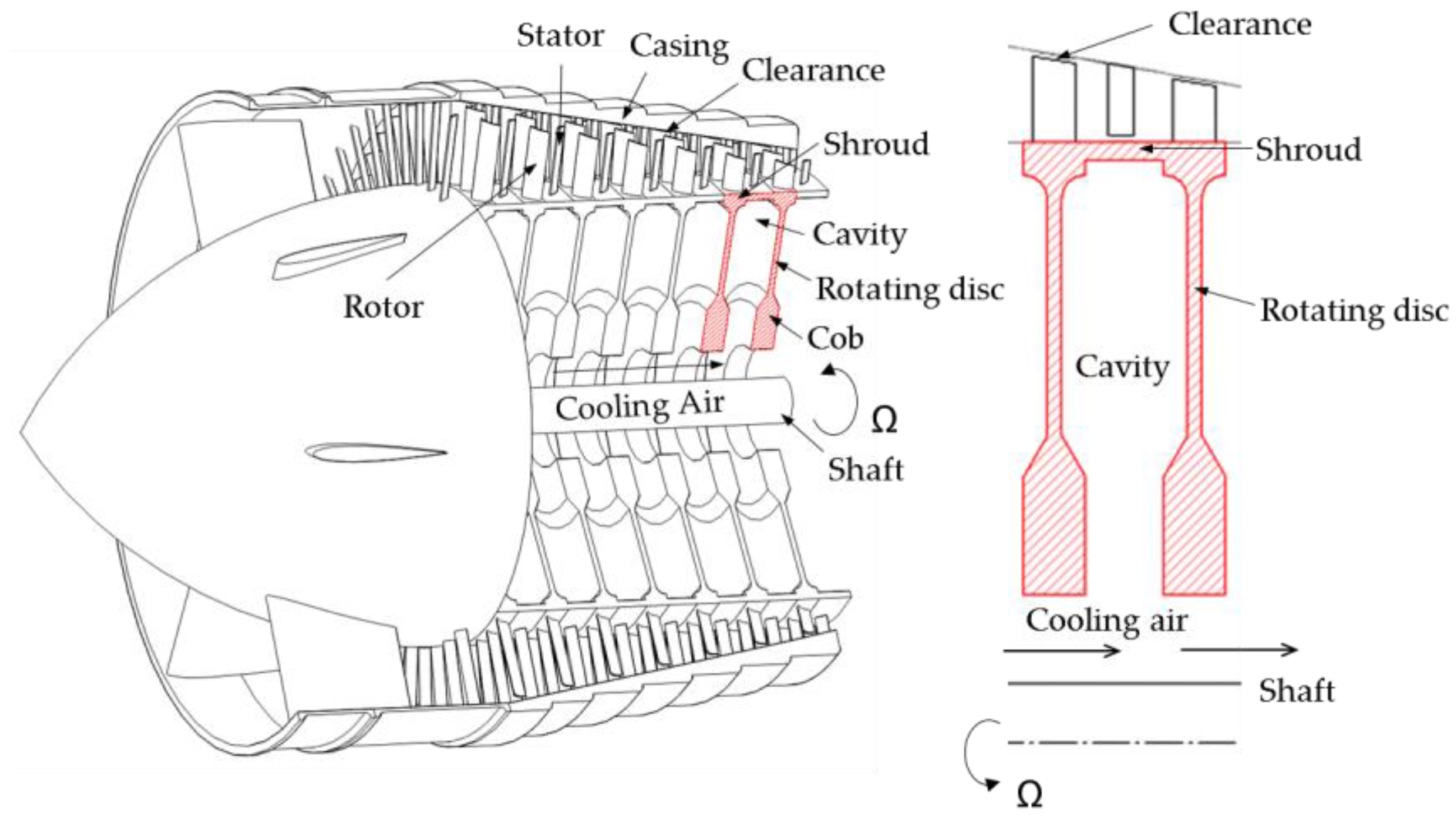
1. Introduction
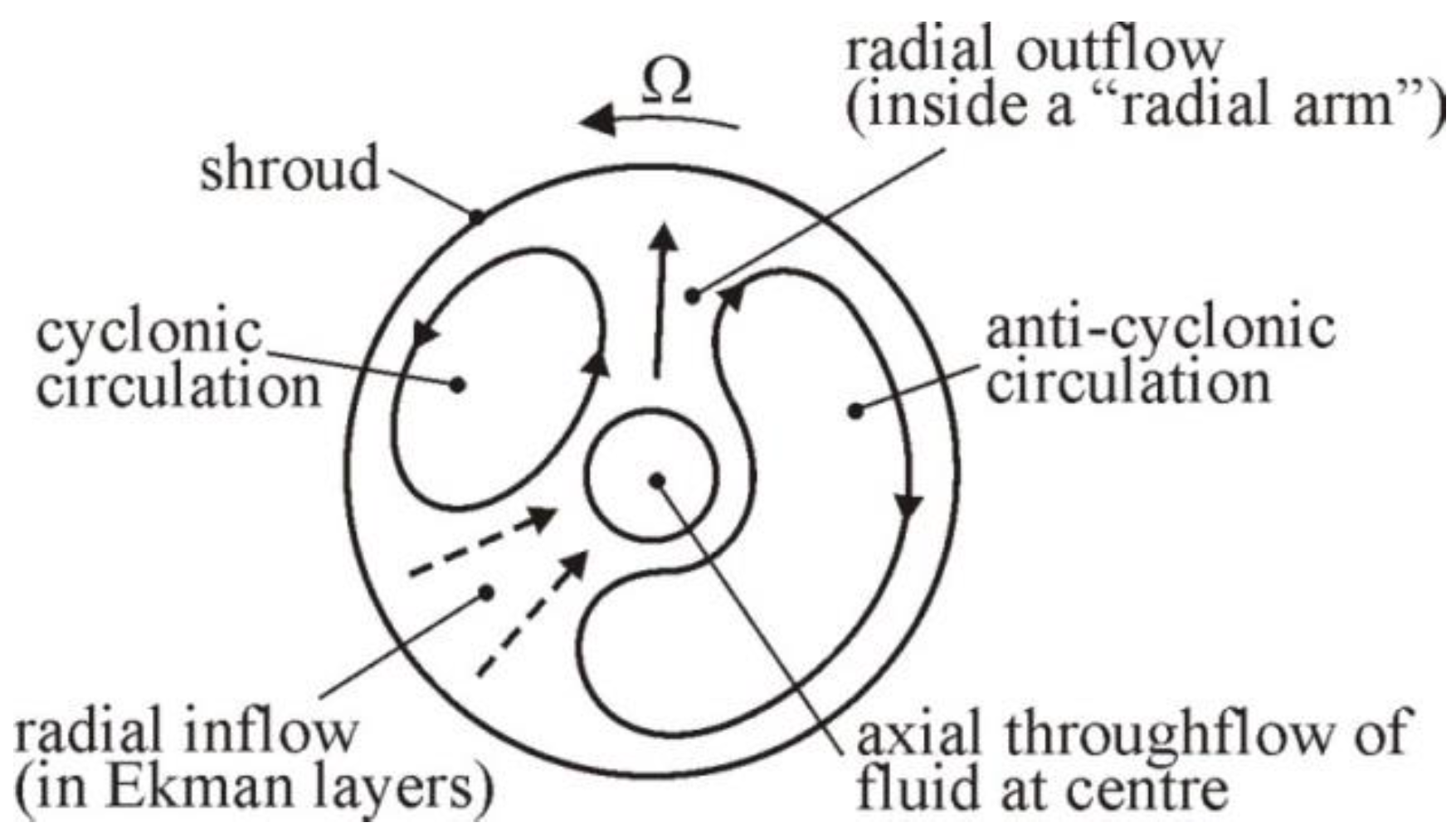
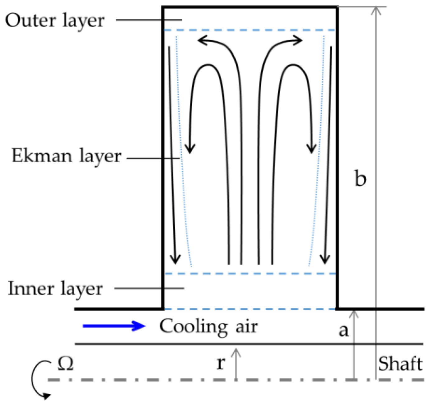
2. Buoyancy-Induced Rotating Flow
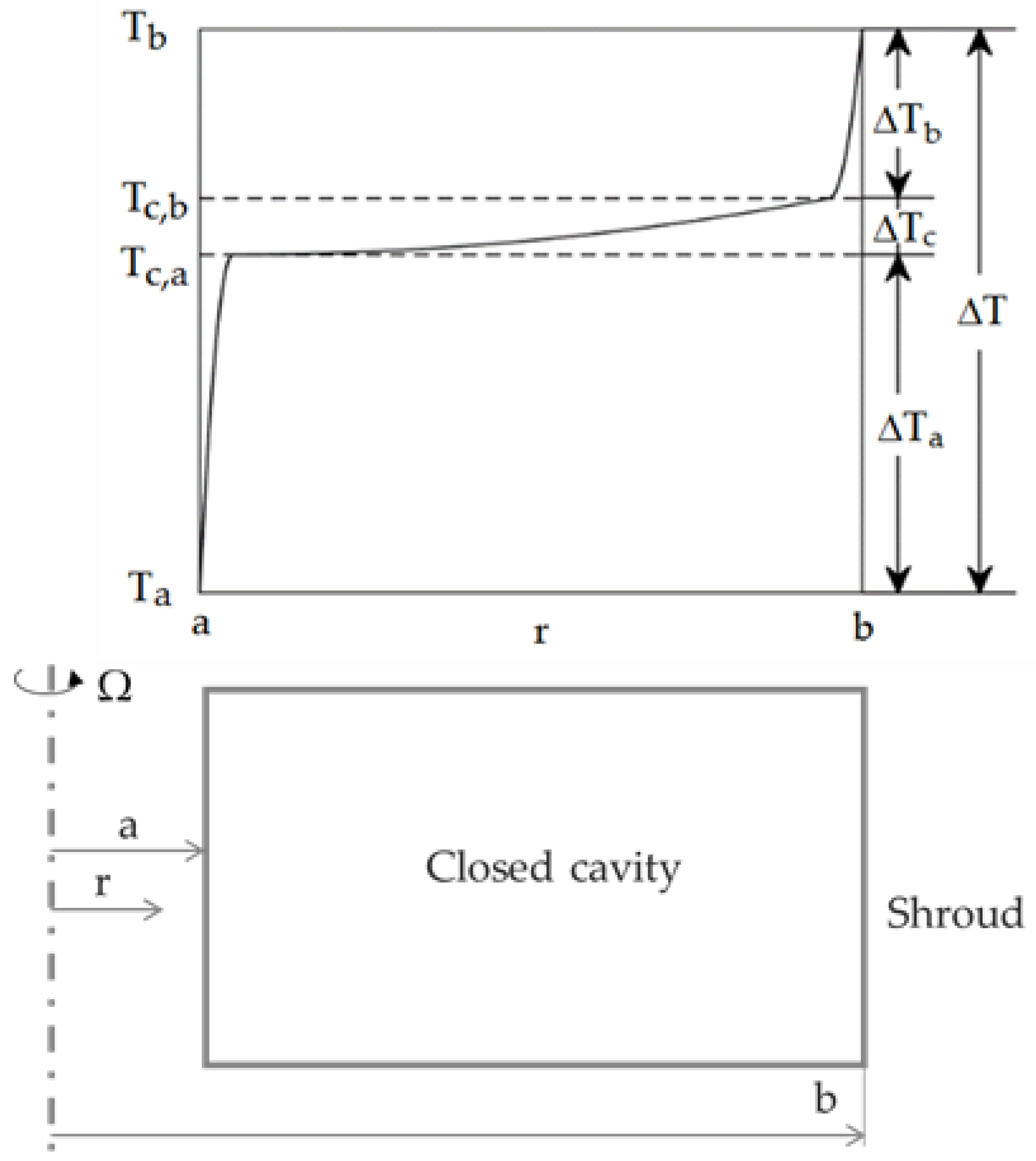
3. Heat Transfer from Shrouds
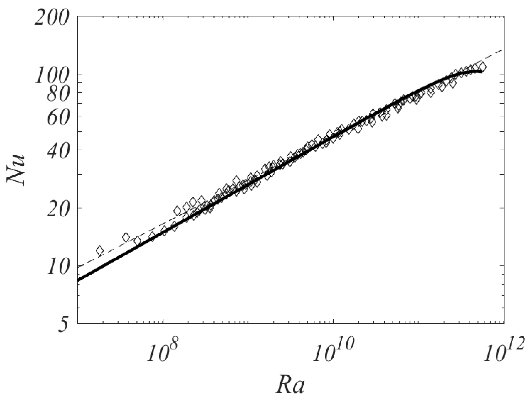
3.1. Calculation of Nusselt Numbers
3.2. Maximum Nusselt Number
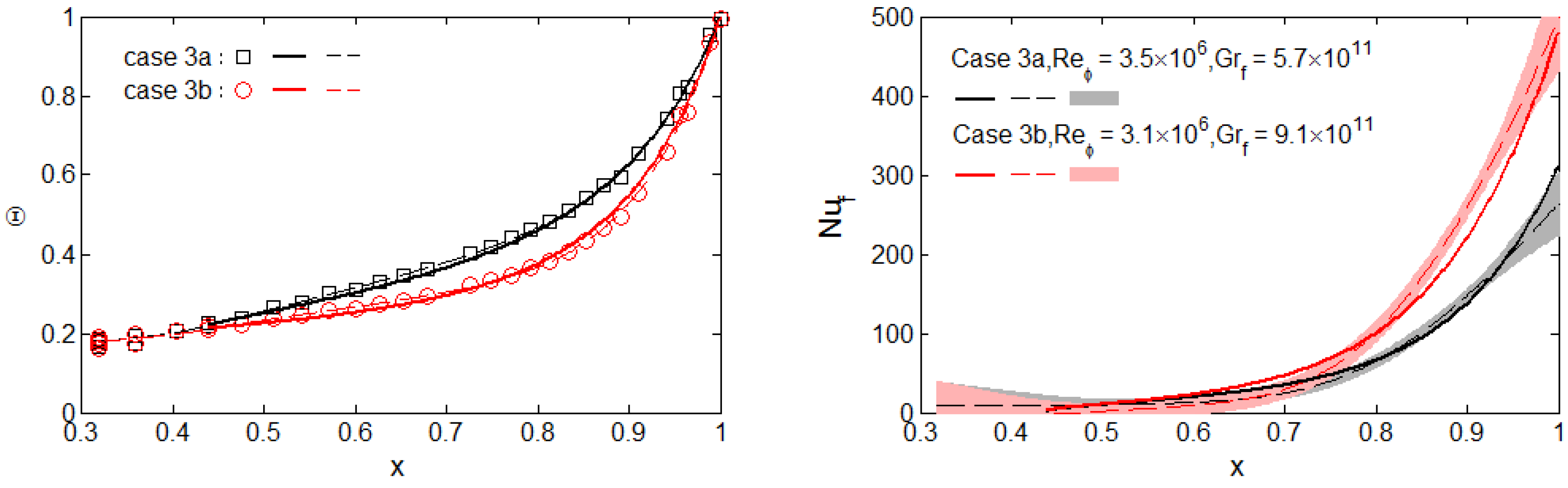
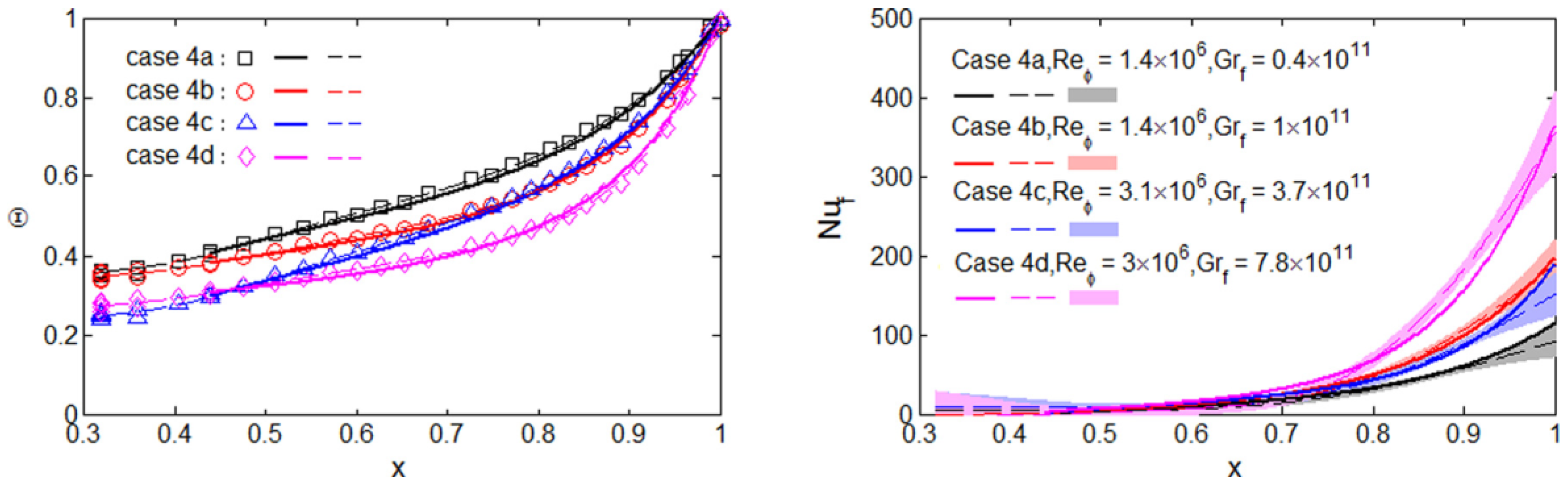
3.3. Comparison with Experimental Measurements
4. Heat Transfer from Discs
4.1. Assumptions for Buoyancy Model
4.2. Modelled Nusselt Numbers
4.3. Modelled Disc Temperatures
4.4. Experimentally Derived Nusselt Numbers and Disc Temperatures
4.5. Comparison with Experimental Measurements
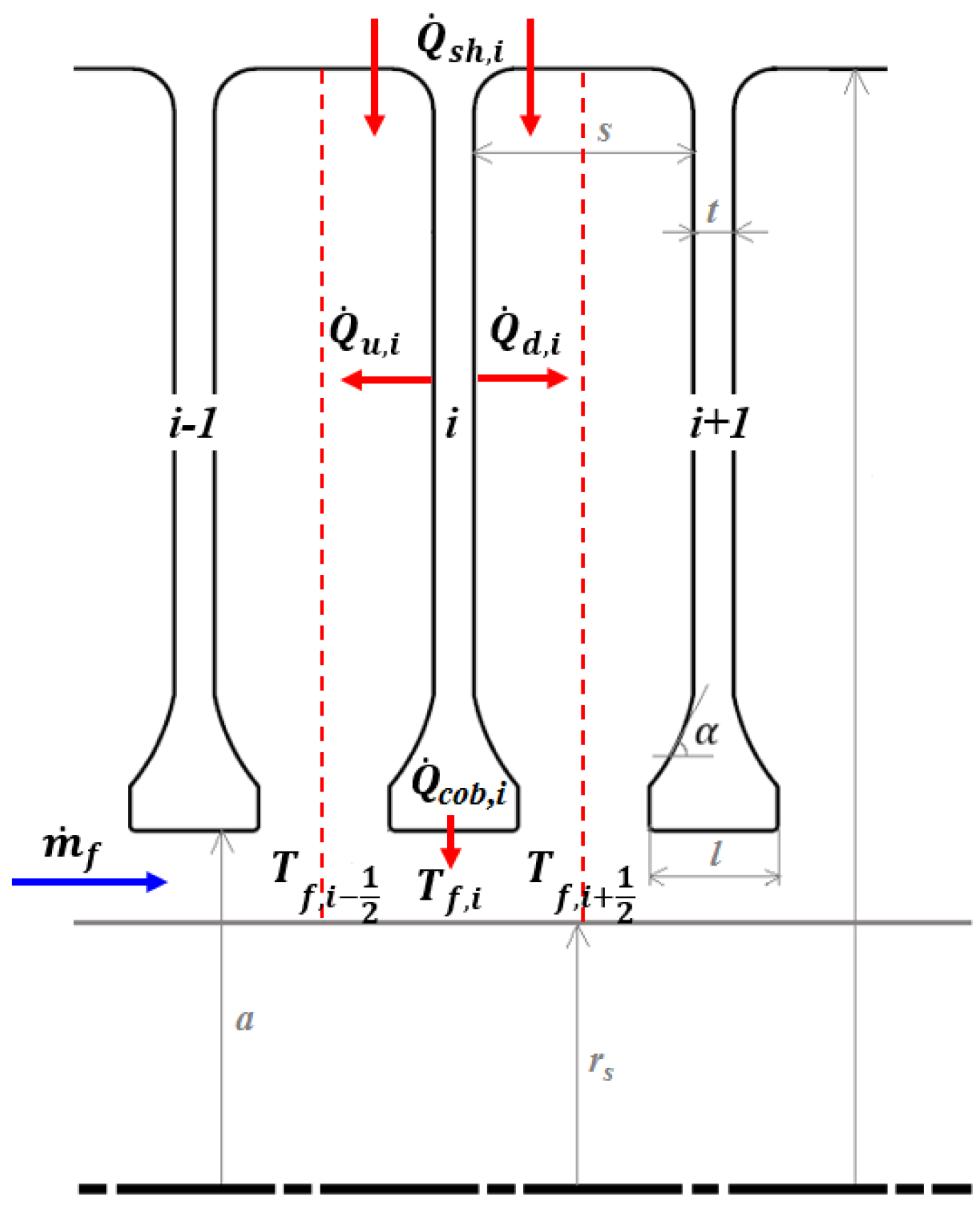
5. Buoyancy-Induced Heat Transfer inside Compressor Rotors
5.1. Model of Heat Transfer from Shroud to Core
5.2. Model of Heat Transfer from Cob to Axial Throughflow
5.3. Model of Temperature Rise of Axial Throughflow
5.4. Comparison between Theoretical and Experimental Values
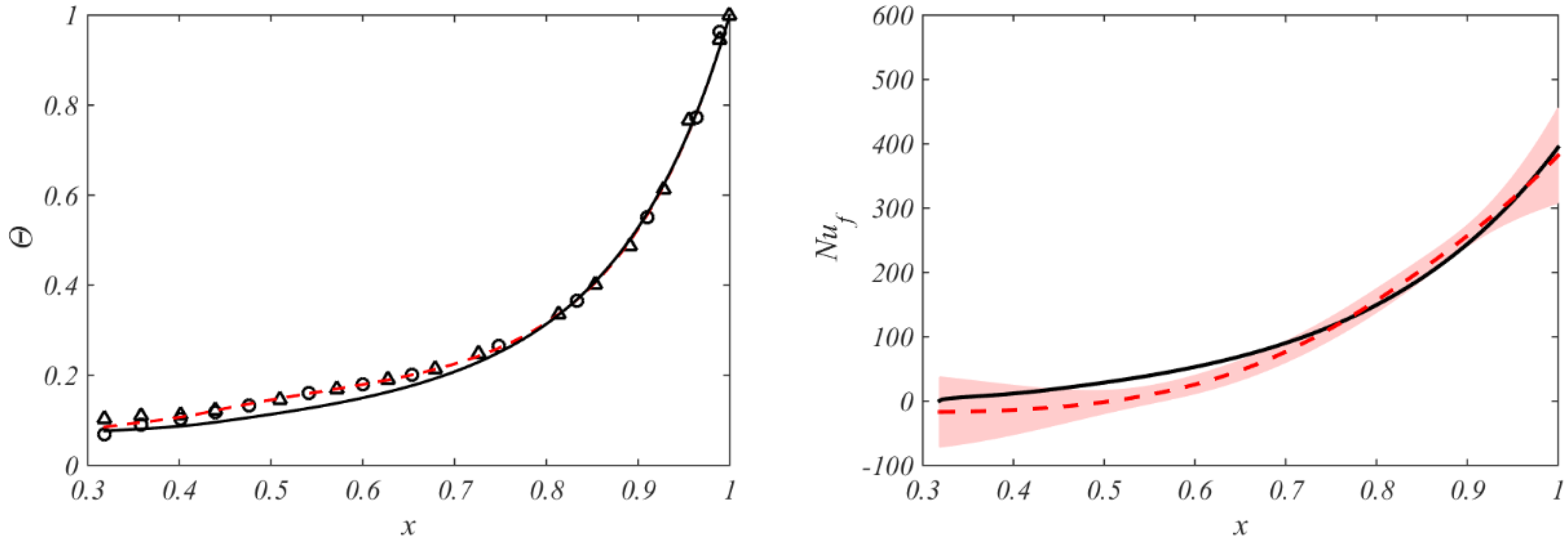
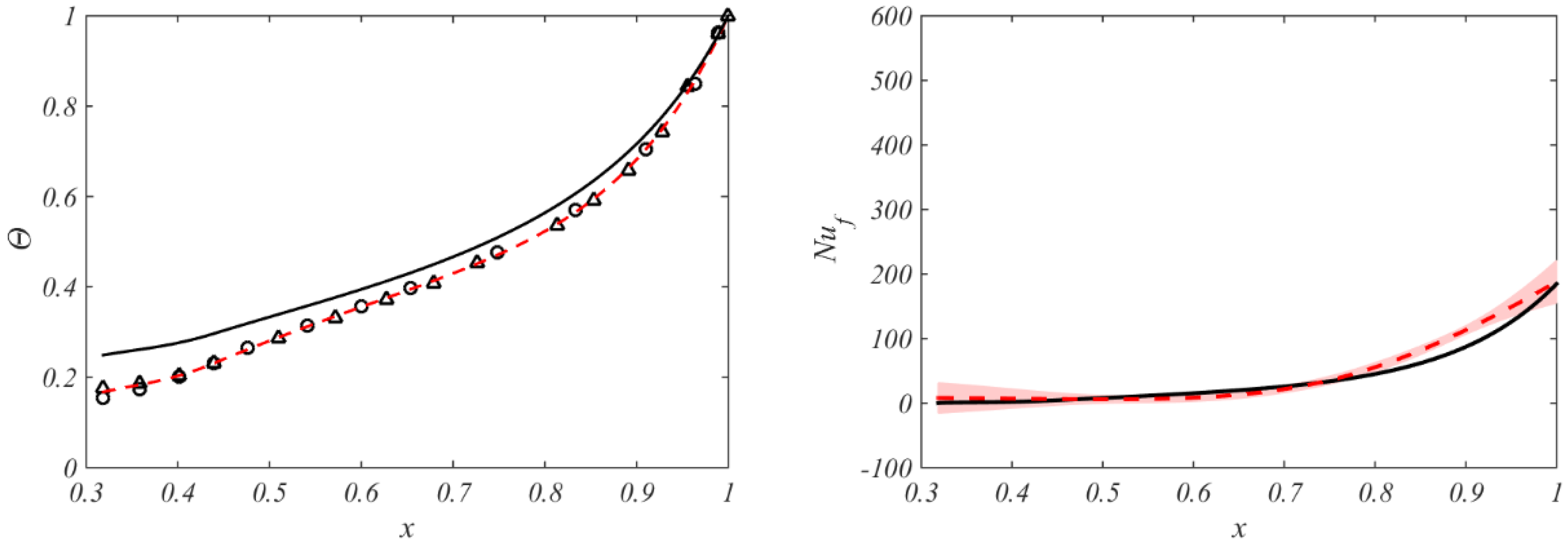
5.4.1. Disc Nusselt Numbers and Temperatures
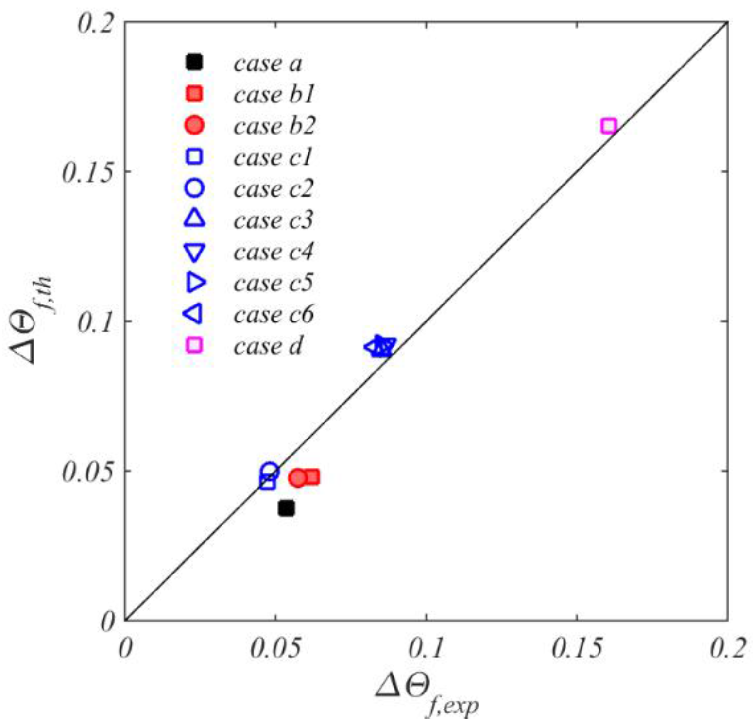
5.4.2. Temperature Rise of Throughflow
6. Conclusions
Acknowledgments
Conflicts of Interest
Nomenclature
| inner radius | |
| inner radius of outer edge of cob | |
| outer radius | |
| empirical constant | |
| empirical constant | |
| specific heat capacity at constant pressure | |
| Coriolis parameter (see Equation (30)) | |
| hydraulic diameter () | |
| Grashof number for closed cavity () | |
| Grashof number of inner surface of closed cavity (see Equation (12)) | |
| Grashof number of outer surface (shroud) of closed cavity (see Equation (13)) | |
| Grashof number in theory (see Equation (29)) | |
| Grashof number in experiment () | |
| shroud Grashof number (see Equation (36)) | |
| heat transfer coefficient | |
| heat transfer coefficient based on (see Equation (26)) | |
| heat transfer coefficient based on () | |
| shroud heat transfer coefficient () | |
| disc number | |
| integral (see Equation (31)) | |
| thermal conductivity of air | |
| thermal conductivity of disc | |
| axial length of cob | |
| characteristic length | |
| characteristic length of inner surface of closed cavity | |
| characteristic length of outer surface of closed cavity | |
| mass flow rate of axial throughflow (kg/s) | |
| Mach number in core (see Equation (A18)) | |
| rotational speed of disc | |
| rotational speed of inner shaft | |
| Nusselt number of closed cavity (see Equation (8)) | |
| Nusselt number of inner surface of closed cavity (see Equation (10)) | |
| Nusselt number of outer surface of closed cavity (see Equation (11)) | |
| Nusselt number based on (see Equation (25)) | |
| cob Nusselt number (see Equation (40)) | |
| Nusselt number based on () | |
| shroud Nusselt number (see Equation (35)) | |
| static pressure | |
| reduced pressure | |
| Prandtl number | |
| heat flux from inner surface of closed cavity to air | |
| heat flux from outer surface of closed cavity to air | |
| heat flux from cob to air | |
| heat flux from disc to air | |
| heat flux from shroud to air | |
| heat flow rate | |
| heat flow rate from inner surface of closed cavity to air | |
| heat flow rate from outer surface of closed cavity to air | |
| heat flow rate from cob to air | |
| heat flow rate due to conduction | |
| heat flow rate from downstream disc surface to air | |
| heat flow rate from upstream disc surface to air | |
| heat flow rate from shroud to air | |
| radius | |
| radius of inner shaft | |
| gas constant | |
| Rayleigh number for close cavity () | |
| critical Ra where reaches maximum | |
| critical Re where reaches maximum | |
| Reynolds number for cob (see Equation (41)) | |
| axial Reynolds number () | |
| rotational Reynolds number based on () | |
| Rossby number () | |
| axial space between discs in cavity | |
| area of convection surface | |
| area of inner surface of closed cavity | |
| area of outer surface of closed cavity | |
| disc thickness | |
| static temperature | |
| temperature of core, throughflow, disc, shroud | |
| circumferential, radial, axial component of velocity in rotating frame | |
| resultant velocity () | |
| speed of sound in core () | |
| axial component of velocity of throughflow | |
| nondimensional radius () | |
| radius ratio () | |
| angle of gradient of disc surface | |
| volume expansion coefficient ) | |
| temperature difference between outer surface and inner surface of closed cavity | |
| temperature difference between core () and inner surface of closed cavity | |
| temperature difference between core () and outer surface of closed cavity | |
| temperature difference between core () and core () | |
| temperature rise of axial throughflow | |
| nondimensional temperature rise of axial throughflow | |
| ratio of specific heats | |
| nondimensional temperature (see Equation (28)) | |
| nondimensional disc temperature () | |
| dynamic viscosity | |
| geometric parameter for close cavity(see Equation (18)) | |
| density | |
| circumferential, radial, axial coordinates | |
| compressibility parameter for close cavity (see Equation (19)) | |
| compressibility parameter for close cavity(see Equation (20)) | |
| angular speed of disc, core | |
| Subscripts | |
| value at | |
| radially-weighted average value | |
| cavity A from [9] | |
| value at | |
| value in core | |
| value on cob | |
| conduction | |
| critical | |
| value on downstream disc surface | |
| Experimentally derived value | |
| value in axial throughflow | |
| values for the disc in a multi-cavity system | |
| value on disc surface | |
| reference value | |
| value on shroud | |
| theoretical or modelled value | |
| value on upstream disc surface | |
| circumferential, radial, axial direction |
Appendix
Linear Equations for Inviscid Rotating Fluids
Compressible Adiabatic Flow in Rotating Core
References
- Owen, J.M.; Long, C.A. Review of buoyancy-induced flow in rotating cavities. J. Turbomach. 2015, 137, 111001. [Google Scholar] [CrossRef]
- Tang, H.; Owen, J.M. Theoretical model of buoyancy-induced heat transfer in closed compressor rotors. J. Eng. Gas Turbines Power 2018, 140, 032605. [Google Scholar] [CrossRef]
- Owen, J.M.; Tang, H. Theoretical model of buoyancy-induced flow in rotating cavities. J. Turbomach. 2015, 137, 111005. [Google Scholar] [CrossRef]
- Tang, H.; Owen, J.M. Effect of buoyancy-induced rotating flow on temperature of compressor discs. J. Eng. Gas Turbines Power 2017, 139, 062506. [Google Scholar] [CrossRef]
- Tang, H.; Shardlow, T.; Owen, J.M. Use of fin equation to calculate nusselt numbers for rotating discs. J. Turbomach. 2015, 137, 121003. [Google Scholar] [CrossRef]
- Tang, H.; Puttock, M.; Owen, J.M. Buoyancy-induced flow and heat transfer in compressor rotors. J. Eng. Gas Turbines Power 2017, in press. [Google Scholar] [CrossRef]
- Farthing, P.R.; Long, C.A.; Owen, J.M.; Pincombe, J.R. Rotating cavity with axial throughflow of cooling air: Flow structure. J. Turbomach. 1992, 114, 237–246. [Google Scholar] [CrossRef]
- Lloyd, J.R.; Moran, W.R. Natural convection adjacent to horizontal surface of various planforms. J. Heat Transf. 1974, 96, 443–447. [Google Scholar] [CrossRef]
- Bohn, D.; Deuker, E.; Emunds, R.; Gorzelitz, V. Experimental and theoretical investigations of heat transfer in closed gas-filled rotating annuli. J. Turbomach. 1995, 117, 175–183. [Google Scholar] [CrossRef]
- Owen, J.M.; Pincombe, J.R.; Rogers, R.H. Source–sink flow inside a rotating cylindrical cavity. J. Fluid Mech. 1985, 155, 233–265. [Google Scholar] [CrossRef]
- Owen, J.M.; Pincombe, J.R. Vortex breakdown in a rotating cylindrical cavity. J. Fluid Mech. 1979, 90, 109–127. [Google Scholar] [CrossRef]
- Atkins, N.R.; Kanjirakkad, V. Flow in a rotating cavity with axial throughflow at engine representative conditions. In Proceedings of the ASME Turbo Expo 2014: Turbine Technical Conference and Exposition, Düsseldorf, Germany, 16–20 June 2014. No. GT2014-27174. [Google Scholar] [CrossRef]
- Long, C.A.; Childs, P.R.N. Shroud heat transfer measurements inside a heated multiple rotating cavity with axial throughflow. Int. J. Heat Fluid Flow 2007, 28, 1405–1417. [Google Scholar] [CrossRef]
- Atkins, N.R. Investigation of a radial-inflow bleed as a potential for compressor clearance control. In Proceedings of the ASME Turbo Expo 2013: Turbine Technical Conference and Exposition, San Antonio, TX, USA, 3–7 June 2013. No. GT2013-95768, V03AT15A020. [Google Scholar] [CrossRef]
- Bohn, D.; Deutsch, G.; Simon, B.; Burkhardt, C. Flow visualisation in a rotating cavity with axial throughflow. In Proceedings of the ASME Turbo Expo 2000: Power for Land, Sea, and Air, Munich, Germany, 8–11 May 2000. GT2000-280. [Google Scholar] [CrossRef]
- Bohn, D.; Dibelius, G.H.; Deuker, E.; Emunds, R. Flow pattern and heat transfer in a closed rotating annulus. J. Turbomach. 1994, 116, 542–547. [Google Scholar] [CrossRef]
- Bohn, D.; Edmunds, R.; Gorzelitz, V.; Kruger, U. Experimental and theoretical investigations of heat transfer in closed gas-filled rotating annuli II. J. Turbomach. 1996, 118, 11–19. [Google Scholar] [CrossRef]
- Bohn, D.; Gier, J. The effect of turbulence on the heat transfer in closed gas-filled rotating annuli. J. Turbomach. 1998, 120, 824–830. [Google Scholar] [CrossRef]
- Bohn, D.; Ren, J.; Tuemmers, C. Investigation of the unstable flow structure in a rotating cavity. In Proceedings of the ASME Turbo Expo 2006: Power for Land, Sea, and Air, Barcelona, Spain, 8–11 May 2006. GT2006-90494. [Google Scholar] [CrossRef]
- Childs, P.R.N. Rotating Flow; Elsevier: Oxford, UK, 2011; ISBN 978-0-123-82098-3. [Google Scholar]
- Dweik, Z.; Briley, R.; Swafford, T.; Hunt, B. Computational study of the heat transfer of the buoyancy-driven rotating cavity with axial throughflow of cooling air. In Proceedings of the ASME Turbo Expo 2009: Power for Land, Sea, and Air, Orlando, FL, USA, 8–12 June 2009. GT2009-59978. [Google Scholar] [CrossRef]
- Farthing, P.R.; Long, C.A.; Owen, J.M.; Pincombe, J.R. Rotating cavity with axial throughflow of cooling air: Heat transfer. J. Turbomach. 1992, 114, 229–236. [Google Scholar] [CrossRef]
- Gunther, A.; Uffrecht, W.; Odenbach, S. Local measurements of disk heat transfer in heated rotating cavities for several flow regimes. J. Turbomach. 2012, 134, 051016. [Google Scholar] [CrossRef]
- Gunther, A.; Uffrecht, W.; Odenbach, S. The effects of rotation and mass flow on local heat transfer in rotating cavities with axial throughflow. In Proceedings of the ASME Turbo Expo 2014: Turbine Technical Conference and Exposition, Düsseldorf, Germany, 16–20 June 2014. GT2014-26228. [Google Scholar] [CrossRef]
- He, L. Efficient computational model for nonaxisymmetric flow and heat transfer in rotating cavity. J. Turbomach. 2011, 133, 021018. [Google Scholar] [CrossRef]
- Hollands, K.G.T.; Raithby, G.D.; Konicek, L. Correlation Equations for Free Convection Heat Transfer in Horizontal Layers of Air and Water. Int. J. Heat Mass Transf. 1975, 18, 879–884. [Google Scholar] [CrossRef]
- Iacovides, H.; Chew, J.W. The computation of convective heat transfer in rotating cavities. Int. J. Heat Fluid Flow 1993, 14, 146–154. [Google Scholar] [CrossRef]
- Johnson, B.V.; Lin, J.D.; Daniels, W.A.; Paolillo, R. Flow characteristics and stability analysis of variable-density rotating flows in compressor-disk cavities. J. Eng. Gas Turbines Power 2006, 128, 118–127. [Google Scholar] [CrossRef]
- King, M.P. Convective Heat Transfer in a Rotating Annulus. Ph.D. Thesis, University of Bath, Bath, UK, 2003. [Google Scholar]
- King, M.P.; Wilson, M. Free convective heat transfer within rotating annuli. In Proceedings of the 12th International Heat Transfer Conference, Grenoble, France, 18–23 August 2002; Volume 2, pp. 465–470. [Google Scholar]
- King, M.P.; Wilson, M. Numerical simulations of convective heat transfer in Rayleigh-Benard convection and a rotating annulus. Numer. Heat Transf. Part A 2005, 48, 529–545. [Google Scholar] [CrossRef]
- King, M.P.; Wilson, M.; Owen, J.M. Rayleigh-Benard convection in open and closed rotating cavities. J. Eng. Gas Turbines Power 2007, 129, 305–311. [Google Scholar] [CrossRef]
- Kumar, V.B.G.; Chew, J.W.; Hills, N.J. Rotating flow and heat transfer in cylindrical cavities with radial inflow. J. Eng. Gas Turbines Power 2013, 135, 032502. [Google Scholar] [CrossRef]
- Lewis, T.W. Numerical Simulation of Buoyancy-Induced Flow in a Sealed Rotating Cavity. Ph.D. Thesis, University of Bath, Bath, UK, 1999. [Google Scholar]
- Long, C.A. Disk heat transfer in a rotating cavity with an axial throughflow of cooling air. Int. J. Heat Fluid Flow 1994, 15, 307–316. [Google Scholar] [CrossRef]
- Long, C.A.; Alexiou, A.; Smout, P.D. Heat Transfer in H.P. Compressor Internal Air Systems: Measurements from the Peripheral Shroud of a Rotating Cavity with Axial Throughflow. In Proceedings of the 2nd International Conference on Heat Transfer, Fluid Mechanics and Thermodynamics (HEFAT 2003), Victoria Falls, Zambia, 23–25 June 2003. Paper No. LC1. [Google Scholar]
- Long, C.A.; Miche, N.D.D.; Childs, P.R.N. Flow measurements inside a heated multiple rotating cavity with axial throughflow. Int. J. Heat Fluid Flow 2007, 28, 1391–1404. [Google Scholar] [CrossRef]
- Long, C.A.; Morse, A.P.; Tucker, P.G. Measurement and computation of heat transfer in high pressure compressor drum geometries with axial throughflow. J. Turbomach. 1997, 119, 51–60. [Google Scholar] [CrossRef]
- Long, C.A.; Tucker, P.G. Numerical computation of laminar flow in a heated rotating cavity with an axial throughflow of air. Int. J. Numer. Methods Heat Fluid Flow 1994, 4, 347–365. [Google Scholar] [CrossRef]
- Long, C.A.; Tucker, P.G. Shroud heat transfer measurements from a rotating cavity with an axial throughflow of air. J. Turbomach. 1994, 116, 525–534. [Google Scholar] [CrossRef]
- Niemela, J.J.; Skrbek, L.; Sreenivasan, K.R.; Donnelly, R.J. Turbulent Convection at Very High Rayleigh Numbers. Nature 2000, 404, 837–840. [Google Scholar] [CrossRef] [PubMed]
- Owen, J.M. Thermodynamic analysis of buoyancy-induced flow in rotating cavities. J. Turbomach. 2010, 132, 031006. [Google Scholar] [CrossRef]
- Owen, J.M.; Abrahamsson, H.; Linblad, K. Buoyancy-induced flow in open rotating cavities. J. Eng. Gas Turbines Power 2007, 129, 893–900. [Google Scholar] [CrossRef]
- Owen, J.M.; Powell, J. Buoyancy-induced flow in a heated rotating cavity. J. Eng. Gas Turbines Power 2006, 128, 128–134. [Google Scholar] [CrossRef]
- Owen, J.M.; Rogers, R.H. Flow and Heat Transfer in Rotating Disc Systems, Volume 2—Rotating Cavities; Research Studies Press: Baldock, UK; John Wiley: New York, NY, USA, 1995; ISBN 086380179X. [Google Scholar]
- Pitz, D.B.; Marxen, O.; Chew, J.W. Onset of convection induced by centrifugal buoyancy in a rotating cavity. J. Fluid Mech. 2017, 826, 484–502. [Google Scholar] [CrossRef]
- Shevchuk, I.V. Convective Heat and Mass Transfer in Rotating Disc Systems; Springer: Heidelberg, Germany, 2009; ISBN 978-3-642-00717-0. [Google Scholar]
- Sun, X.; Kilfoil, A.; Chew, J.W.; Hills, N.J. Numerical simulation of natural convection in stationary and rotating cavities. In Proceedings of the ASME Turbo Expo 2004: Power for Land, Sea, and Air, Vienna, Austria, 14–17 June 2004. GT2004-53528. [Google Scholar] [CrossRef]
- Sun, X.; Linblad, K.; Chew, J.W.; Young, C. LES and RANS investigations into buoyancy-affected convection in a rotating cavity with a central axial throughflow. J. Eng. Gas Turbines Power 2007, 129, 318–325. [Google Scholar] [CrossRef][Green Version]
- Tan, Q.; Ren, J.; Jiang, H. Prediction of flow features in rotating cavities with axial throughflow by RANS and LES. In Proceedings of the ASME Turbo Expo 2009: Power for Land, Sea, and Air, Orlando, FL, USA, 8–12 June 2009. GT2009-59428. [Google Scholar] [CrossRef]
- Tan, Q.; Ren, J.; Jiang, H. Prediction of 3D unsteady flow and heat transfer in rotating cavity by discontinuous Galerkin method and transition model. In Proceedings of the ASME Turbo Expo 2014: Turbine Technical Conference and Exposition, Düsseldorf, Germany, 16–20 June 2014. GT2014-26584. [Google Scholar] [CrossRef]
- Tian, S.; Tao, Z.; Ding, S.; Xu, G. Investigation of flow and heat transfer in a rotating cavity with axial throughflow of cooling air. In Proceedings of the ASME Turbo Expo 2004: Power for Land, Sea, and Air, Vienna, Austria, 14–17 June 2004. GT2004-53525. [Google Scholar] [CrossRef]
- Tritton, D.J. Physical Fluid Dynamics; OUP: New York, NY, USA, 1988; ISBN 0-19-854489-8. [Google Scholar]
- Tucker, P.G. Temporal behaviour of flow in rotating cavities. Numer. Heat Transf. Part A 2002, 41, 611–627. [Google Scholar] [CrossRef]


| Cases | Ro ≈ 5 | Ro ≈ 1 | Ro ≈ 0.6 | Ro ≈ 0.3 | |||||||||||||||
|---|---|---|---|---|---|---|---|---|---|---|---|---|---|---|---|---|---|---|---|
| 1a | 1b | 1c | 1d | 1e | 1f | 2a | 2b | 2c | 2d | 2e | 2f | 2g | 3a | 3b | 4a | 4b | 4c | 4d | |
| 4.7 | 4.7 | 4.9 | 4.9 | 4.5 | 4.5 | 0.8 | 0.8 | 0.9 | 0.9 | 1.0 | 1.0 | 1.0 | 0.6 | 0.6 | 0.3 | 0.3 | 0.3 | 0.3 | |
| 0.0017 | 0.0030 | 0.0085 | 0.015 | 0.062 | 0.14 | 0.065 | 0.10 | 0.44 | 0.84 | 1.7 | 2.5 | 3.9 | 5.7 | 9.1 | 0.4 | 1.0 | 3.7 | 7.8 | |
| 0.078 | 0.077 | 0.19 | 0.19 | 0.46 | 0.45 | 0.46 | 0.45 | 1.1 | 1.1 | 2.1 | 2.1 | 2.1 | 3.5 | 3.1 | 1.4 | 1.4 | 3.1 | 3.0 | |
| 0.08 | 0.17 | 0.05 | 0.11 | 0.09 | 0.24 | 0.09 | 0.16 | 0.11 | 0.23 | 0.13 | 0.19 | 0.32 | 0.15 | 0.32 | 0.06 | 0.16 | 0.12 | 0.29 | |
| 0.19 | 0.19 | 0.50 | 0.50 | 1.1 | 1.1 | 0.19 | 0.18 | 0.51 | 0.50 | 1.1 | 1.1 | 1.1 | 1.1 | 1.1 | 0.20 | 0.20 | 0.48 | 0.48 | |
| 28.7 | 30.7 | 51.6 | 58.2 | 92.3 | 109 | 47.4 | 53.4 | 96.7 | 126 | 131 | 170 | 233 | 126 | 225 | 45.3 | 82.5 | 72.1 | 146 | |
| 32.5 | 37.2 | 56.2 | 66.5 | 103 | 128 | 59.4 | 64.7 | 109 | 135 | 149 | 175 | 216 | 133 | 214 | 50.5 | 83.5 | 78.0 | 142 | |
| Case | Ro ≈ 0.6 | Ro ≈ 0.3 | Ro ≈ 0.2 | Ro ≈ 0.1 | ||||||
|---|---|---|---|---|---|---|---|---|---|---|
| a | b1 | b2 | c1 | c2 | c3 | c4 | c5 | c6 | d | |
| Ro | 0.61 | 0.31 | 0.31 | 0.16 | 0.16 | 0.18 | 0.17 | 0.17 | 0.17 | 0.10 |
| Grf/1011 | 2.5 | 10 | 10 | 4.2 | 4.5 | 6.8 | 7.2 | 7.2 | 7.8 | 4.1 |
| 0.32 | 0.35 | 0.35 | 0.15 | 0.16 | 0.33 | 0.32 | 0.32 | 0.34 | 0.29 | |
| Reϕ/106 | 1.6 | 3.0 | 3.0 | 3.0 | 3.0 | 2.5 | 2.7 | 2.7 | 2.7 | 2.1 |
| Rez/104 | 5.1 | 5.0 | 5.0 | 2.5 | 2.5 | 2.4 | 2.4 | 2.4 | 2.5 | 1.1 |
| 1.0 | 0.34 | 1.0 | 0.34 | −0.34 | 1.0 | 0.34 | −0.34 | 0 | 0 | |
| 0.347 | 0.349 | 0.330 | 0.499 | 0.494 | 0.357 | 0.377 | 0.385 | 0.368 | 0.413 | |
| 0.334 | 0.332 | 0.334 | 0.540 | 0.518 | 0.364 | 0.370 | 0.367 | 0.357 | 0.427 | |
© 2018 by the authors. Licensee MDPI, Basel, Switzerland. This article is an open access article distributed under the terms and conditions of the Creative Commons Attribution (CC BY) license (http://creativecommons.org/licenses/by/4.0/).
Share and Cite
Owen, J.M.; Tang, H.; Lock, G.D. Buoyancy-Induced Heat Transfer inside Compressor Rotors: Overview of Theoretical Models. Aerospace 2018, 5, 32. https://doi.org/10.3390/aerospace5010032
Owen JM, Tang H, Lock GD. Buoyancy-Induced Heat Transfer inside Compressor Rotors: Overview of Theoretical Models. Aerospace. 2018; 5(1):32. https://doi.org/10.3390/aerospace5010032
Chicago/Turabian StyleOwen, J. Michael, Hui Tang, and Gary D. Lock. 2018. "Buoyancy-Induced Heat Transfer inside Compressor Rotors: Overview of Theoretical Models" Aerospace 5, no. 1: 32. https://doi.org/10.3390/aerospace5010032
APA StyleOwen, J. M., Tang, H., & Lock, G. D. (2018). Buoyancy-Induced Heat Transfer inside Compressor Rotors: Overview of Theoretical Models. Aerospace, 5(1), 32. https://doi.org/10.3390/aerospace5010032