CFD Validation and Flow Control of RAE-M2129 S-Duct Diffuser Using CREATE^TM-AV Kestrel Simulation Tools

Abstract

The flow physics modeling and validation of the Royal Aircraft Establishment (RAE) subsonic intake Model 2129 (M2129) are presented. This intake has an 18 inches long S duct with a 5.4 inches offset, an external and an internal lip, forward and rear extended ducts, and a center-positioned bullet before the outlet. Steady-state and unsteady experimental data are available for this duct. The measurements include engine face conditions (pressure recovery, static pressure to free-stream total pressure ratio, and distortion coefficient at the worst 60${}^{\circ }$ sector or DC60), as well as wall static pressure data along the duct. The intake has been modeled with HPCMP CREATE${}^{\mathrm{TM}}$-AV Kestrel simulation tools. The validation results are presented including the effects of turbulence models on predictions. In general, very good agreement (difference errors are less than 6%) was found between predictions and measurements. Secondary flow at the first bend and a region of flow separation are predicted at the starboard wall with an averaged DC60 coefficient of 0.2945 at the engine face. Next, a passive and an active flow control method are computationally investigated. The passive one uses vane-type vortex generators and the active one has synthetic jet actuators. The results show that considered passive and active flow control methods reduce the distortion coefficient at the engine face and the worst 60${}^{\circ }$ sector to 0.1361 and 0.0881, respectively. The flow control performance trends agree with those obtained in experiments as well. These results give confidence to apply the Kestrel simulation tools for the intake design studies of new and unconventional vehicles and hence to reduce the uncertainties during their flight testing.

1. Introduction

A key challenge in the development of an aircraft is to integrate the propulsion system with the airframe such that a balance between the integrated propulsion requirements and the overall aircraft design demands are met. Many of the engineering challenges in this issue arise from the fact that the successful integration of airframes and engines involves major compromises between the wishes of the aircraft and engine manufacturers. For a multi-mission aircraft propulsion system, the installation study involves the design of intake, exhaust system, secondary air system (i.e., ejector nozzles), and the integration of those components with the engine and aircraft.

Typically, the intake design is the aircraft manufacturer’s responsibility, but in terms of the installed-engine performance, the intake effects need to be understood. The optimal intake design is a trade-off study about desirable requirements, namely high pressure recovery, low installation drag, low radar and noise signatures, as well as minimum weight and cost. In terms of propulsion, the function of the intake is to introduce a sufficient mass of air from the ambient environment flow uniformly and with stability to the engine compressor under all flight conditions.

Turbojet and low bypass turbofan engines are often located within the fuselage of an aircraft. This is especially employed in combat aircraft which should face a compact layout in order to reduce radar cross section. In addition, this type of engine installation results in less installation drag. However, the optimal incorporation of an engine into the aircraft fuselage for reducing the radar cross-section is a complex task because such a configuration requires an S duct with the possibility of thick boundary layer ingestion into the engine compressor under the severe conditions of the adverse pressure gradient inside the duct. Thus, the design of these intakes must ensure that the engine operates effectively in the presence of such boundary-layer ingestion and to avoid significant flow distortion. The intake flow distortion is characterized by the non-uniformity in the flow parameters (such as velocity and pressure) in planes perpendicular to the flow direction [1]. Specifically, flow distortions at the engine face should be minimized. In a subsonic intake diffuser, the flow distortion is caused by the ingestion of fuselage boundary layer or aircraft vortices into intake, flow separation at the cowl lips during maneuvering conditions, or formation of secondary and separated flow regions at the intake bends with small radius of curvature. These airflow distortions will lead to total pressure loss and non-uniformity at the engine face which reduces the compressor surge margin and may eventually cause the compressor to stall, engine instability, and the performance deviation from design conditions [2]. Careful consideration should therefore be given to the design of the shape of the cowl lip and diffuser of these intakes.

The purpose of this article is to determine the flow characteristics of S duct intakes via the extensive use of computational simulations. The Computational Fluid Dynamic (CFD) tools, however, need to be first verified against experimental data. In order to verify the used CFD tools, the Royal Aircraft Establishment (RAE) subsonic intake Model 2129 (M2129) is considered here. This subsonic S duct intake was designed under a joint program between NASA and the UK Ministry of Defense (MOD) and was tested in the DRA/Bedford wind tunnel. The aim of these experiments was to calibrate CFD codes and achieve the inlet distortion control.

The flow inside M2129 S-duct intake has been extensively studied using experimental and numerical methods. However, all CFD codes based on solutions of the Reynolds-Averaged Navier-Stokes (RANS) equations failed to exactly predict measured data because of the complexity of flow-field inside this duct [3,4]. As detailed in Ref. [5], the flow initially accelerates before reaching the throat section of this intake. At the first bend, the flow passing along the starboard side (inside of the bend) is subject to the centrifugal and pressure forces which cause the flow streamlines move towards the port side (outside of the bend). The interaction of the incoming flow from the inner side with the adverse pressure gradient region occurring at the port side leads to forming two swirling secondary flows. The flow continues to decelerate inside the diffuser and the ram pressure will rise as well. At the second bend, the low (kinetic) energy flow at the outside wall does not form any strong secondary flows that balance or cancel those generated by the first bend. In addition, the low energy flow along the starboard side of the second bend is subject to adverse pressure gradient region and will separate. Most CFD codes using RANS solutions failed to predict the observed secondary flows and the exact location of flow separation point. However, hybrid RANS and large eddy simulation methods have improved these predictions. This work in particular focuses on the simulation of the RAE M2129 intake using the HPCMP (High Performance Computing Modernization Program) CREATE${}^{\mathrm{TM}}$-AV (Air Vehicles) Kestrel simulation tools. These relatively new tools from the U.S. DoD (Department of Defense) HPCMP have extensively been tested and validated for a wide range of external flow applications, however, much less effort has been devoted to the validation of the code for internal flow problems.

It is quite impossible to design an S duct diffuser with small flow distortions at all flight conditions. Therefore, many studies have focused on the reduction and control of intake flow distortion using passive [6,7] and active flow controls [8,9]. The most common methods for passive and active controls are using vanes/plates and synthetic jet actuators, respectively. Passive vortex generators have already been used to control the boundary layer separation in many applications. The mixture of low and high momentum flow regions by these devices can locally control the effects of separation. Vane-type vortex generators have been used in S duct intakes as well to improve pressure recovery, for example see Ref. [10]. The recent applications of these devices attempt to improve both total pressure recovery and uniformity. In these applications, an array of vane type vortex generators are typically placed at or behind the first bend to control the secondary flow formation [11]. Though these devices are very simple to install, they cannot effectively control and reduce distortion at all off-design conditions.

Anderson and Gibb [11] presented the experimental results of applying different vortex generator configurations for the secondary flow control of the M2129 S duct. The experiments were again conducted at the DRA/Bedford 13 ft × 9 ft wind tunnel with the throat Mach number in range of 0.2 to 0.8. The VG170 configuration of Anderson and Gibb’s study is considered in this work. This configuration has the best performance among others for all tested conditions. It consists of 22 vanes with chord length ratio of 0.2703 and blade height ratio of 0.07.

Air jet vortex generators have been tested for the flow control of the M2129 S duct as well [12]. These devices are more difficult to install than passive ones and require bleeding high pressure air from engine that might affect its performance. However, these devices lead to lower distortion coefficients and improve engine face conditions at all off-design conditions. In this work, an active control method with 22 jets is considered; each jet has a diameter of 1 mm, an imping angle of 30 degrees relative to the walls, with a bled air total to free-stream pressure ratio of two.

This work uses the HPCMP CREATE${}^{\mathrm{TM}}$-AV Kestrel simulation tools to validate and investigate the flow predictions of the RAE M2129 S duct baseline. Computational tools are then investigated for studying the distortion and flow changes of this baseline with vane type and air jet vortex generators. The article is organized as follows. First, CFD solver and test cases are described. The intake performance is briefly presented. Next, the validation results are given for the baseline followed by the results obtained from baseline with control methods. Finally, concluding remarks are provided.

2. CFD Solver

The simulation tools used in this work is the fixed wing computational tool of CREATE${}^{\mathrm{TM}}$-AV program, i.e., Kestrel. The code is a DoD-developed solver in the framework of the CREATE${}^{\mathrm{TM}}$ Program, which is funded by the DoD High Performance Computing Modernization Program (HPCMP). The CREATE${}^{\mathrm{TM}}$ focuses on addressing the complexity of applying computationally based engineering to improve DoD acquisition processes [13]. CREATE${}^{\mathrm{TM}}$ consists of three computationally based engineering tool sets for design of air vehicles, ships, and radio-frequency antennae. The fixed wing analysis code, Kestrel, is part of the Air Vehicles Project (CREATE${}^{\mathrm{TM}}$-AV) and is a modularized, multidisciplinary, virtual aircraft simulation tool incorporating aerodynamics, jet propulsion integration, structural dynamics, kinematics, and kinetics [13]. The code has a Python-based infrastructure that integrates Python, C, C++, or Fortran-written components [14]. New modules can easily integrated into the code.

Kestrel version 7.2 is used in this work. The flow solver of the code discretizes Reynolds–Averaged Navier Stokes (RANS) equations into a cell-centered finite-volume form. The code then solves unsteady, three-dimensional, compressible RANS equations on hybrid unstructured grids [15]. The Method of Lines (MOL) in the code separates temporal and spatial integration schemes from each other [16]. The spatial residual is computed via a Godunov type scheme [17]. Second-order spatial accuracy is obtained through a least squares reconstruction. The numerical fluxes at each element face are computed using various exact and approximate Riemann schemes with a default method based on HLLE++ scheme [18]. In addition, the code uses a subiterative, point-implicit scheme method (a typical Gauss-Seidel technique) to improve the temporal accuracy.

Kestrel receives an eXtensible Markup Language (XML) input file generated by Kestrel User Interface and stores the solution convergence and volume results in a common data structure for later use by the Output Manager component. Some of the turbulence models available within Kestrel include the one-equation turbulence models of Spalart–Allmaras (SA) [19], Spalart–Allmaras with rotational/curvature correction (SARC) [20], Mentor’s SST model [21], and Delayed Detached Eddy Simulation (DDES) with SARC [22] and SST RANS turbulence model [21].

3. Test Case

An S-duct diffuser, named RAE M2129, was designed around 1990 under a joint program between NASA and the UK defense Ministry and was tested in the DRA/Bedford 13 ft × 9 ft wind tunnel. A large number of diffuser geometries have been studied with different lip shapes, cross-sectional changes, and etc. The test case used in this study corresponds to the geometry used in the Aerodynamics Action Group AD/AG-43, “Application of CFD to High Offset Intake Diffusers” [23]. The aim of this project was calibration of CFD codes for an S duct diffuser.

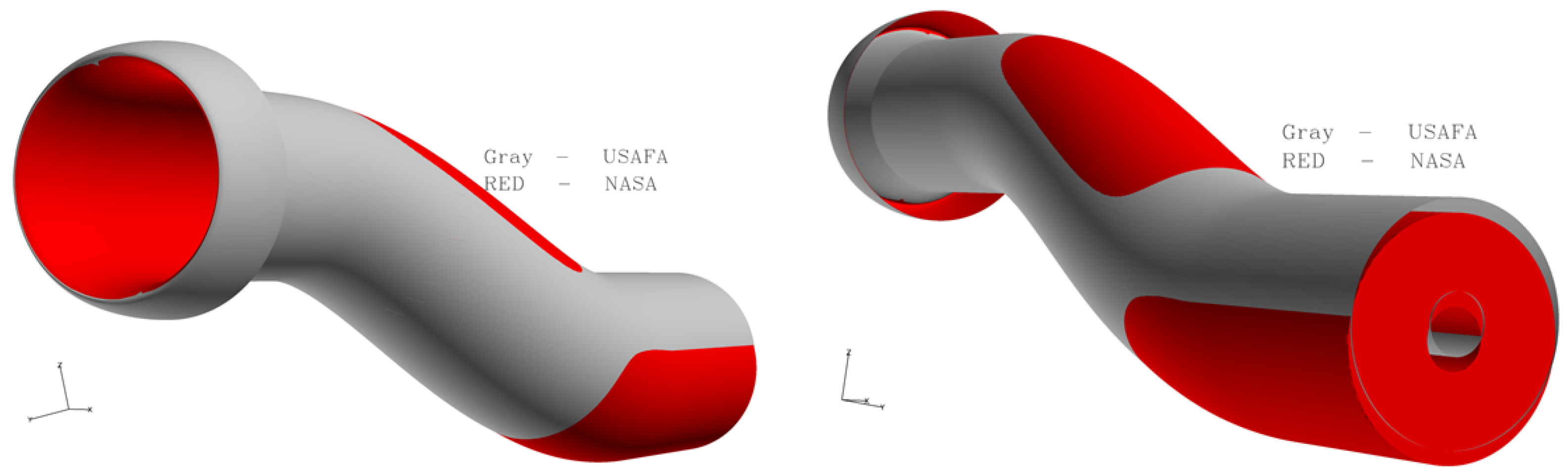
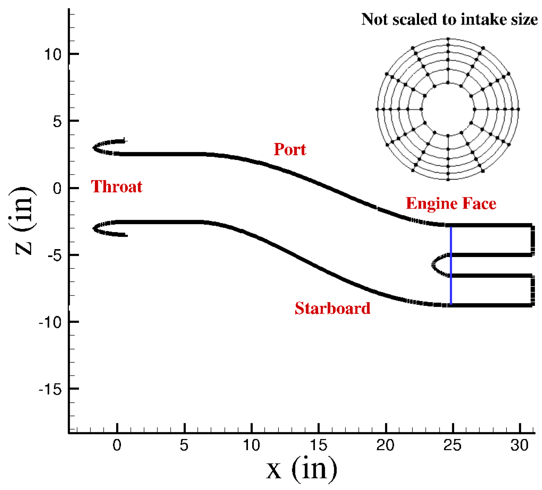
The M2129 geometry is shown in Figure 1. This intake has a circular entry section followed by an S bend diffuser. The model is a side-mounted duct with a horizontal plane of symmetry, i.e., $y=0$. The diffuser offset is therefore in the horizontal plane. Based on this setup, the duct side with minimum z was named starboard, port was the side with the maximum z, the minimum y side was named bottom, and finally the maximum y side top.

The inlet throat diameter is approximately 5.06 inches. The diffuser length is 18 inches with 5.4 inches centerline offset. Two constant-area sections were added at the upstream and end of the duct as shown in Figure 1. With this modification the overall built duct length was 29.969 inches. The engine face bullet starts at $x=23.129$ inches measured from the most forward part of the intake lip and becomes parallel at $x=24.569$ inches. The engine face, where measurements were made, is at $x=24.669$ inches as well. In more detail, the locus of the centerline offset curve and the variation of the radius in the diffusing part of the intake can be determined by following equations:

$$\begin{array}{ccc}\hfill z& =& 0.15L\left[1-cos\left(\pi {\displaystyle \frac{x}{L}}\right)\right]\hfill \end{array}$$

(1)

$$\begin{array}{ccc}\hfill \left({\displaystyle \frac{R-R_t}{R_f-R_t}}\right)& =& 3{\left(1-{\displaystyle \frac{x}{L}}\right)}^4-4{\left(1-{\displaystyle \frac{x}{L}}\right)}^3+1\hfill \end{array}$$

(2)

where L is the diffuser length, $R_t$ and $R_f$ are the throat and engine face radii, respectively. By studying these equations, the 5.4 inches be deduced to be the duct offset between the throat and engine face center.

The RAE M2129 intake experiments were conducted in the DRA/Bedford 13 ft × 9 ft wind tunnel which is a closed-circuit type. The experimental data used in this work corresponds to Data Point (DP) 78. The diffuser of this run has a bullet and a static rake in the compressor entry plane. The free-stream conditions in these experiments correspond to a Mach number of 0.204 and zero angles of attack and side slip. Free-stream total pressure and total temperature were 105,139.5 Pa and 293.7 K, respectively.

Table 1. Flow conditions of the DP78 run of RAE-M2129 baseline.

Flow Conditions	Experimental Data
Free-stream Mach	0.204
Free-stream total pressure	105,139.5 Pa
Free-stream total temperature	293.7 K
Angle of attack	0 degree
Sideslip angle	0 degree
Mass flow ratio	1.9382

lists all experimental conditions. The static rake at the engine face (see Figure 1) had 12 equally spaced arms with 30 degrees intervals, such that each arm had six pitot pressure probes. The inner probes were at 1.1 inches radius, while the outer probes were positioned at a radius of 2.89 inches. The measurements included pressure recovery, static pressure to total free-stream pressure, and DC60 coefficient at the engine face. In additions, DP78 experiments had four rows of static pressure taps along the duct at starboard, port, top, and bottom sides.

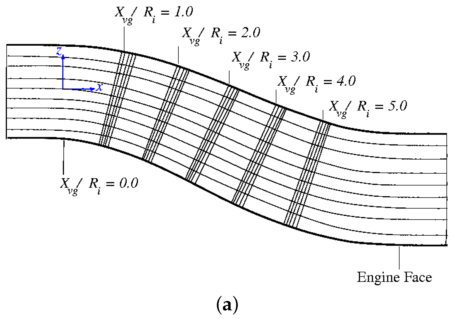
In a different experimental campaign by Gibb and Anderson [12], the RAE M2129 diffuser was tested with different vane type vortex generator designs. The general geometries of these vanes and their locations relative to the diffuser entry plane are given in Ref. [12] and shown in Figure 2. In this work, the VG170 configuration is used. Referring to Figure 2, this configuration has 22 vanes located at $X_{VG}/R_i$ of 2.0. Each vane has a blade height ratio ($h/R_i$) of 0.070 and chord length ratio ($c/R_i$) of 0.2703. In addition, the spacing angle and the vane angle of attack were set at 15${}^{\circ }$ and 16${}^{\circ }$, respectively.

Finally, the M2129 diffuser intake with air jet vortex generators (AJVG) was studied as well. Experimental data of such a flow control method were again reported by Gibb and Anderson [12]. In the present work, similar designs to Ref. [12] are used as well. The flow control consists of the row of high pressure jets located in the position of VG170 vane-equipped configuration described earlier. Unlike the designs used in Ref. [12], the jets of this work are inclined 17 degrees towards the inlet wall and 30 degrees towards the surface normal direction following recommendation of Ref. [24]. The jet diameters are 1 mm as well.

4. Computational Grids

Four grids are considered in this study. Detail of these grids are given in

Table 2. Detail of computational grids.

Grid	Description	Number of Cells (Millions)
Grid1	Obtained from NASA; baseline intake	31.2
Grid2	generated at USAFA; baseline intake	15
Grid3	generated at USAFA; baseline intake + 22 vanes	19.9
Grid4	generated at USAFA; baseline intake + 22 jets	62.3

. The first grid corresponds to the RAE M2129 wind tunnel geometry without any flow control. This corresponds to the wind tunnel model of DP78 run with a bullet. However, the computational model has slightly longer forward extension than the section of experimental model. The grid for this geometry is a hybrid (structured and unstructured) and was obtained from Bernhard Anderson of NASA Glenn Research Center and has about 31.2 million cells. This grid has structured cells over all wall surfaces. Body-fitted structured grid layers exist at the wall and tetrahedra cells used elsewhere. This model was used for CFD validation of the M2129 diffuser baseline.

A second intake diffuser was modeled at the U.S. Air Force Academy (USAFA) using M2129 intake data and Equations (1) and (2). These two geometries (USAFA and NASA) do not match everywhere as shown in Figure 3. The new geometry has slightly different offset from the original one and the cross-sectional changes are different from experimental models as well.

Three grids were then made from this new intake geometry: one without any flow control, one with passive, and one with active flow control. Geometry and grids are shown in Figure 4. The passive flow control consist of one row of vanes which are designed according to Ref. [12] and its detailed VG170 configuration. The grid generator builds a prism layer around the vane surfaces to enable their modeling as viscous wall. The active flow control consists of the row of high pressure jets located in the position of VG170 vanes configuration as well.

The computational grids were made in Pointwise version 18. Most of the surface mesh is made of patches of structured mesh with prism layers build upon the surface mesh. The remaining parts of interior meshes above the prism layer are made of tetra cells. The thickness of the first layer is determined by the condition of y+ < 1 with a cell wall normal growth ratio of 1.25. The baseline grid has approximately 15 million cells. The approximate numbers of cells for intake with passive and active controls are 19.9 and 62.3 million cells, respectively.

5. Intake Performance

In general, the loss of total pressure inside a diffuser intake can be the result of the wall frictions, the flow separation, and formation of shock waves. A term named pressure recovery can represent the level of losses of a diffuser. It is defined as follows:

$$PR={\displaystyle \frac{p_{0f}}{p_{0\infty }}}$$

(3)

where $p_{0f}$ is the mean total pressure at the engine’s face plane and $p_{0\infty }$ denotes free-stream total pressure. If the diffuser flow is assumed to be isentropic, there is no pressure losses and the outlet and inlet total pressures of the intake are the same which gives a pressure recovery of one. Wallin et al. [25] presented a relationship between the pressure recovery and geometric patterns of a not bent intake. Based in this relationship, as the duct length increases, the pressure losses will rise due to the higher skin friction losses. These pressure losses will be higher if the intake has a bend and when the internal cross-section shape changes, e.g., from elliptic to circular. In addition, the pressure recovery values drop if the engine operates at the larger throttle setting. The pressure recovery will fall off with increasing yaw and incidence angle as well. Additionally, the influence of external pressure field (wing, fuselage, etc.) upon the intake pressure recovery needs to be determined. For the intake types that the entry is from fuselage, the run up distance and wetted fuselage area ahead of intake significantly affect the flow-field inside the intake. The prediction of all these effects upon the intake’s performance is a challenging task that must be concerned within the intake performance analysis.

The sensitivity of the engine performance on the intake’s pressure-recovery depends on the design of the engine. Antonatos et al. [26] have assumed a linear relationship between the total pressure losses and the engine thrust as:

$${\displaystyle \frac{▵F}{F}}=CR·\left(1-PR\right)$$

(4)

where $▵F$ and F denote thrust drop and thrust force respectively. $CR$ is the correction factor that depends on the engine configuration. The correction factor for turbojet and turbofan engines lies between 1.1 and 1.6 over the Mach number range 0.8 to 2.2.

In addition to the total pressure losses, the diffuser flow is distorted where the flow separates from boundary surfaces or in the presence of secondary flows. The separation in duct can be result of sharp bends, thin lip, shock and boundary-layer interactions and etc. Since the 1950s, the following distortion parameter is used widely to identify distortion level:

$$D_t={\displaystyle \frac{p_{0f,\max }-p_{0f,\min }}{p_{0f}}}$$

(5)

where the maximum and minimum total pressures are taken from a series of measurements of equally spaced radial probes around the engine face plane. Later, new distortion definitions were used based on the differential total pressure values between the probes average and minimum pressure total pressures. Different distortion coefficients have been defined as well. The one that has been adopted in this study is from Ref. [23] which is defined as:

$$DC60={\displaystyle \frac{p_{0f}-p_{0f,60}}{{\overline{q}}_f}}$$

(6)

where $p_{0f,60}$ is the mean total pressure in the worst 60-degree sector of the engine face. ${\overline{q}}_f$ is the mean dynamic pressure at the engine face as well.

6. Results and Discussions

Computational resources were provided by the DoD’s High Performance Computing Modernization Program. All simulations are run on the Engineering Research Development Center (ERDC) Topaz System (3456 computing nodes with 36 cores per node running two Intel Xeon E5-2699v3 processors at a base core speed of 2.3 GHz with 117 GBytes of RAM available per node). Each job asks for 2024 computing nodes and 8 h wall-clock time. The convergence criterion is based on tracking data (CFD parameters, coefficients, forces) that Kestrel prints at each time step and whether the averaged values have reached a converged state or not.

Validation results use the NASA baseline grid without any flow control mechanism. Kestrel was used to solve the flow inside this intake diffuser. The boundary conditions for the far-field included the free-stream Mach number, total pressure and total temperature corresponding to DP78 experimental data of Ref. [23]. These data are given in Table 1. The outlet plane was defined as a sink boundary with the given mass flow rate of Table 1.

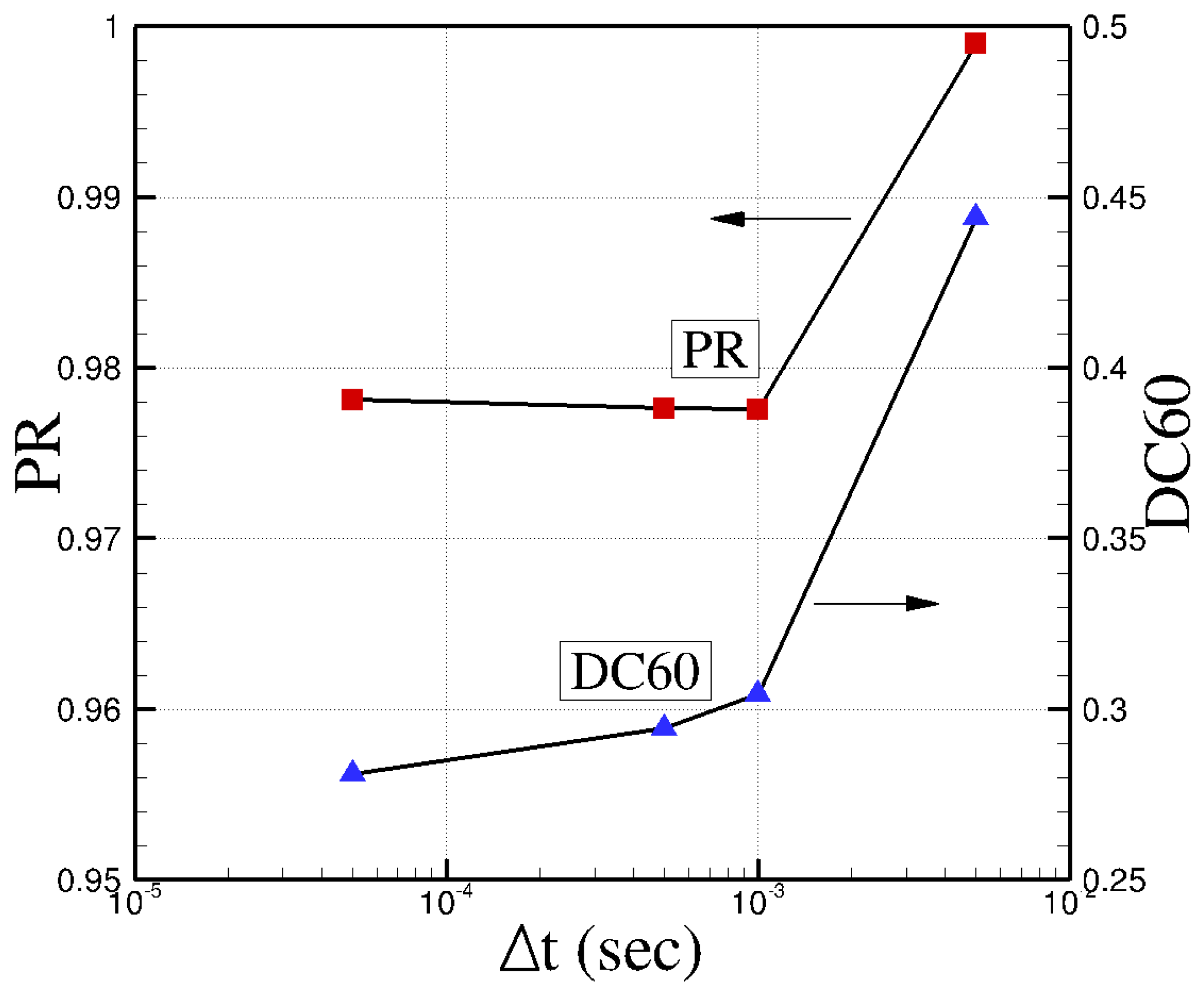
All CFD simulations are run in unsteady mode with second order accuracy in time and three Newton subiterations as recommended by the Kestrel user guide [27]. A global time step of $5\times {10}^{-4}$ s is used in all simulations. Notice that the accuracy of predictions of secondary and separated flows inside a S duct will largely depend on the temporal order of accuracy and selected time step. Too large the time step can cause instability, inaccuracy, and not capturing important time-dependent features. Too small the time step will increase the computational cost to simulate flow changes over a given period of time. In order to understand the effects of time step on the solution, pressure recovery and DC60 values of simulations of the NASA baseline grid using SARC–DDES turbulence model are plotted versus time step in Figure 5. Note that all simulations were run for 2.25 s of physical time; the solutions between 2 and 2.25 s were then time-averaged. Figure 5 shows that pressure recovery and DC60 values have nearly converged to their final values and experimental data for a time step of $5\times {10}^{-4}$ s. Interestingly, the values corresponding to the smallest time step used, i.e., $1\times {10}^{-5}$ s, show slightly larger differences with experimental data than the selected time step of $5\times {10}^{-4}$ s. In addition, CFD data using this small time step are ten times more expensive to obtain.

All simulations are initially run with 500 startup iterations and then are continued for 4500 regular time steps or 2.25 s of physical time. Note that during startup iterations, simulation time remains zero. Time-averaged data are then written for last 500 time steps or simulation times between 2 and 2.5 s. Two sets of tap positions are defined: In the first, tap points are located at the engine face and correspond to the pitot tube locations of a static rake used in the DP78 experimental run. This rake has six pitot pressure probes at each of 12 equally spaced arms with 30 degrees intervals, i.e., 72 tap positions. These tap positions are shown in Figure 1. The second set of tap data correspond to the intake wall at starboard and port sides. These taps were generated using Carpenter, a mesh manipulation tool of Kestrel, as the result of the symmetry plane cut with the duct wall. Density, static and total pressure, and velocity components at each tap positions are written by the solver for each time step from 4000 to 4500. Finally, simulations are run for different turbulence models.

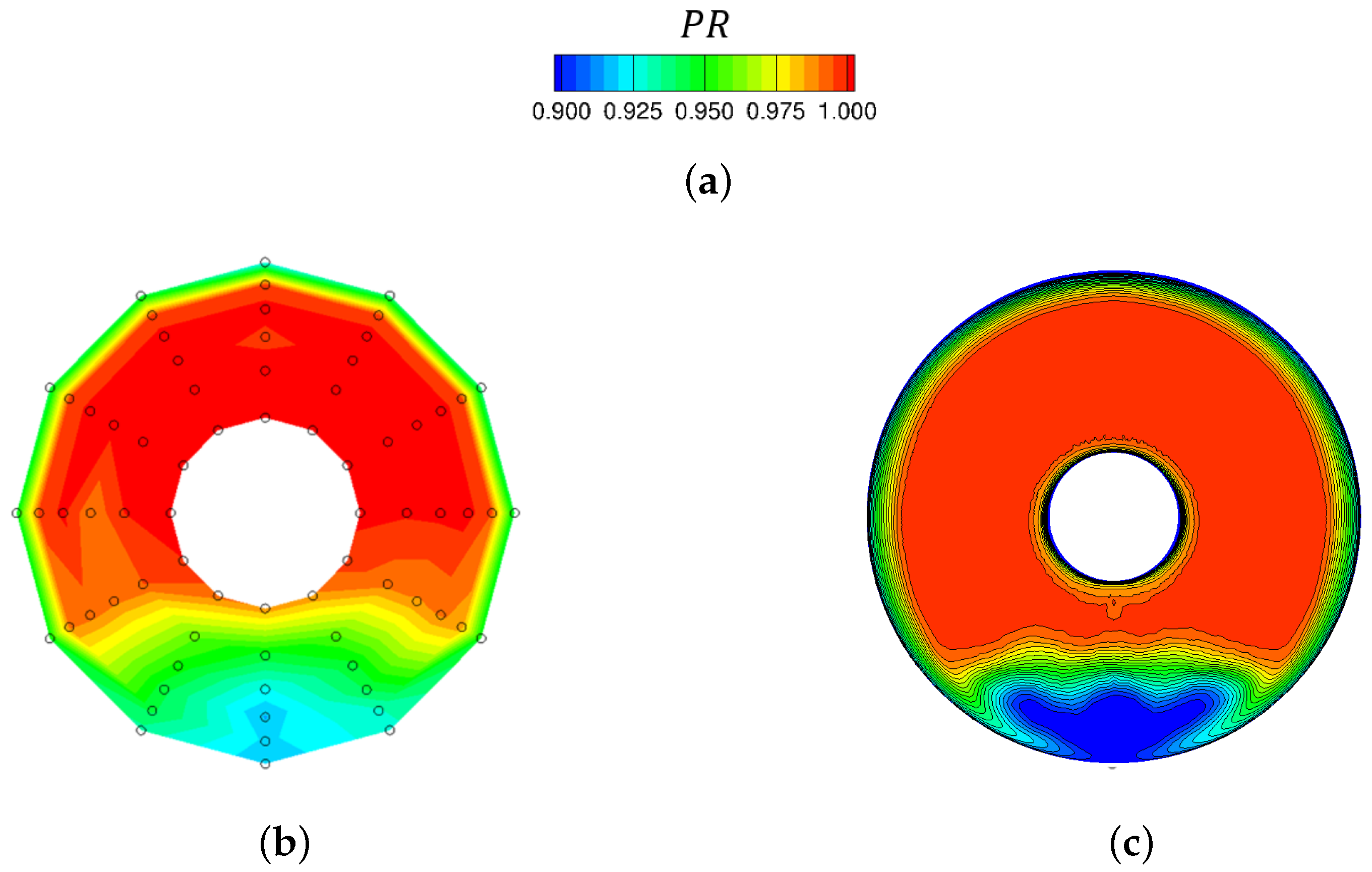
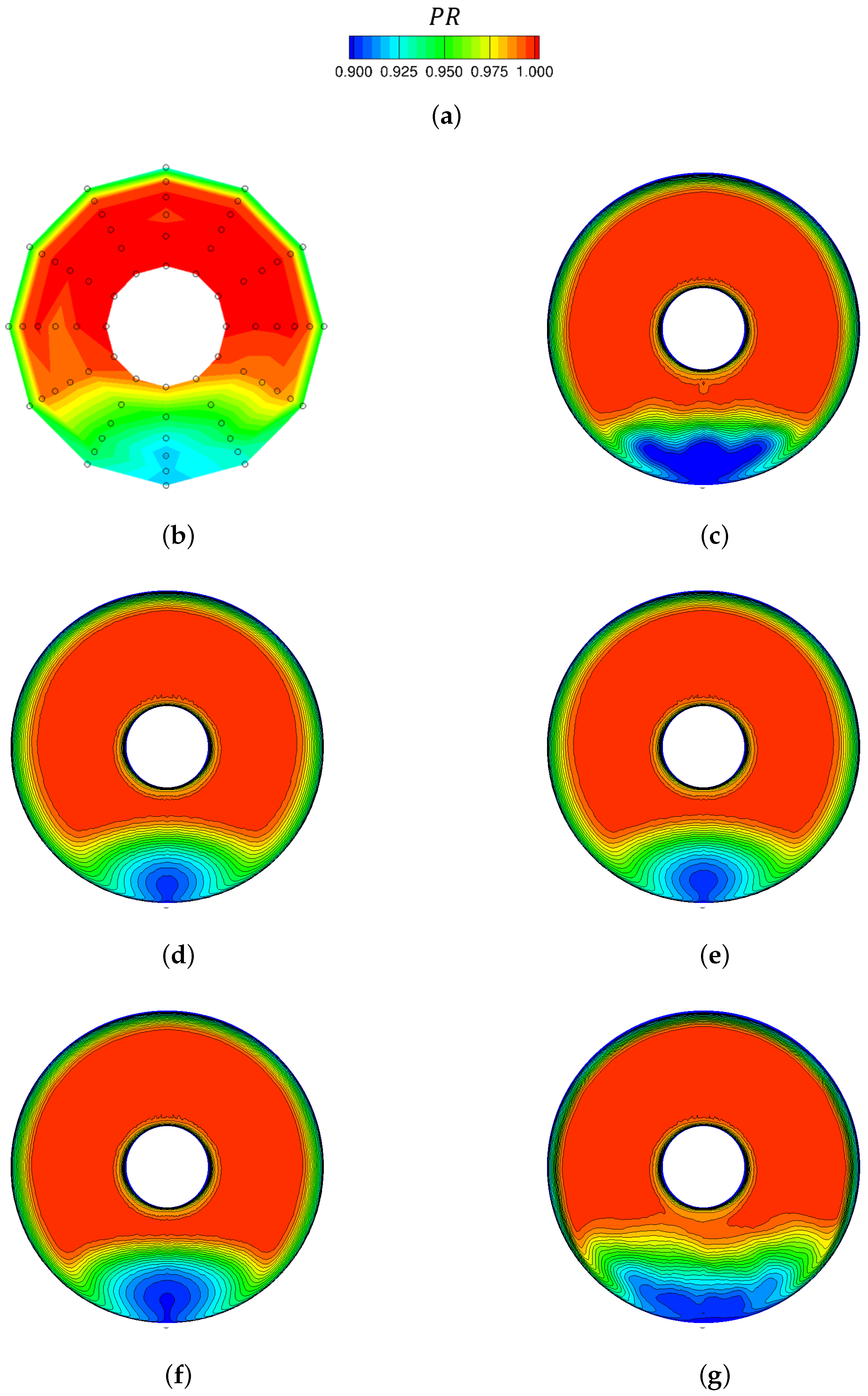
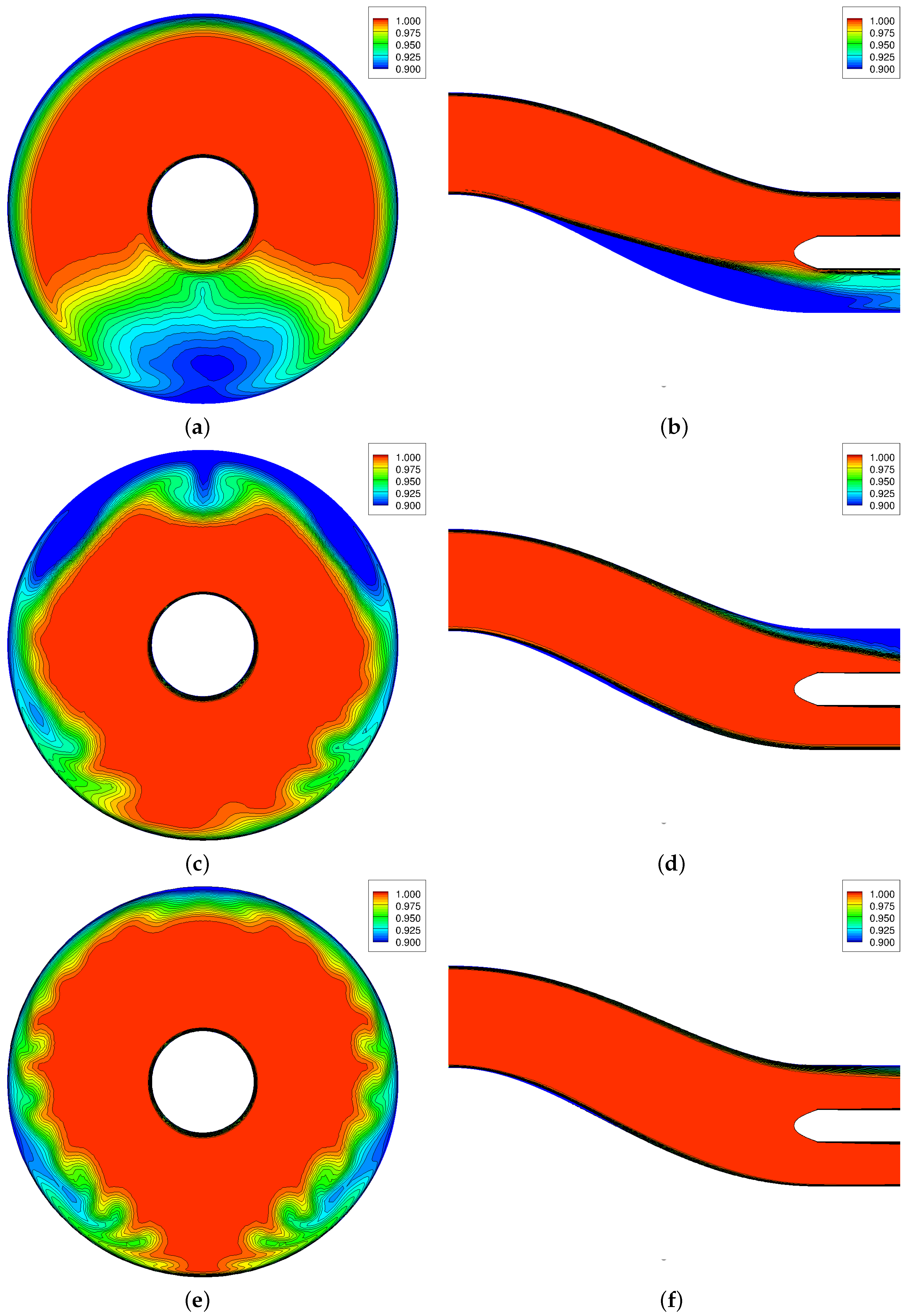
First set of results compare the time-averaged pressure recovery (total pressure to free-stream total pressure) at the engine face with available experimental data measured at pitot pressure probes. The comparison plots are shown in Figure 6 using the SARC–DDES turbulence model. Time-averaged data are plotted using visualization files with averaged data from simulation times between 2 to 2.5 s. Notice that measurements were taken at shown pitot pressure probes of Figure 6b and therefore the shown experimental plot is a partial representation of the actual engine face, e.g., the bullet is not shown. Additionally, pressure recovery data at regions between arms or measurements were interpolated from the rake measured data. However, CFD data show the full engine face plane generated in TECPLOT.

Figure 6 shows that overall pressure recovery trends predicted by CFD solver are similar to those found in the experiments. Pressure recovery values at and near walls are small because of skin friction effects. There is a separated flow region at the starboard side of the engine face plane with low pressure recovery values which make non-uniform flow entering the engine compressor. At this region (blue-colored region of Figure 6), there are two large counter-rotating vortices near the intake’s symmetry plane and at the starboard side of intake. Two smaller secondary vortices are formed outside and above the primary vortices as well (these vortices are not shown in the figure). These vortices were not well captured with the experiments using shown static probes.

In more detail,

Table 3. Validation data of the RAE-M2129 baseline intake. NASA grid was used with SARC–DDES turbulence model. CFD data are time-averaged from 2 to 2.5 s of simulation time.

Engine Face Station	Experimental Data	CFD Data (Rake)	CFD Data (Face)	Error (Rake), $\mathit{\epsilon }$ %
$p_{0f}/p_{0\infty }$	0.9744	0.9776	0.9752	−0.328
Mach No.	0.4193	0.4329	0.4329	−3.243
$p_f/p_{0\infty }$	0.8522	0.8737	0.8497	−2.523
DC60	0.3130	0.2945	0.3294	5.910

compares Kestrel predictions using SARC-DDES with available measurements of DP78 run. CFD data are again time-averaged values for simulation times between 2 to 2.5 s. These averaged data are calculated in two ways. In the first approach, CFD data (total, static pressure, density, velocities) are written at each rake point shown in Figure 7 and then used to find engine face conditions. These data are available at each time step from time 2 to 2.5 s meaning that the tap data in CFD are reported for last 500 time steps. A script was then written to find averaged pressure recovery, Mach, static pressure ratio and DC60 coefficient at the engine face using these data.

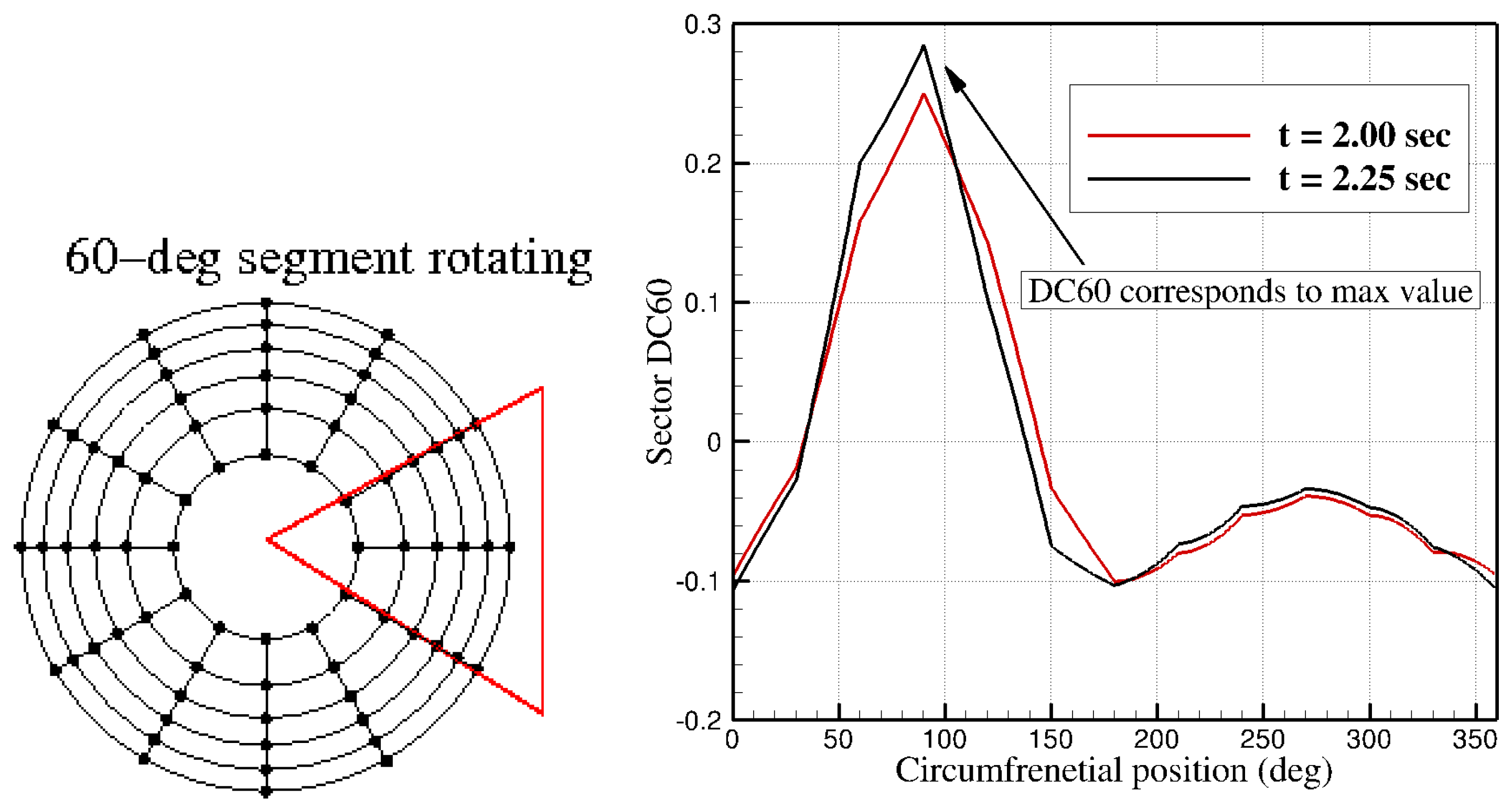
The process of calculating DC60 from pressure rakes is illustrated in Figure 7. In more detail, the inputs to the code are flow conditions at locations of the shown rake probes. The number of probes is specified as a number of arms of the rake probe and a number of probes at each arm. DC60 index is then calculated for a 60 degrees sector rotating clockwise, one degree at each time. The swirl index and DC60 then corresponds to the critical sector with maximum DC60 index value. The data can be steady or a sequence of time dependent solutions. In addition, the utility saves flow field data for visualization purposes in Ensight format. In the second method, the engine face conditions are estimated from engine face data input in TECPLOT. Time-averaged solutions are used for this purpose. Table 3 shows that CFD data are about 6% of measured data. This is perhaps one of the best matches seen for this run. Both methods (rake and face data) agree well to each other but DC60 values are slightly overpredicted using the face data compared with rake data.

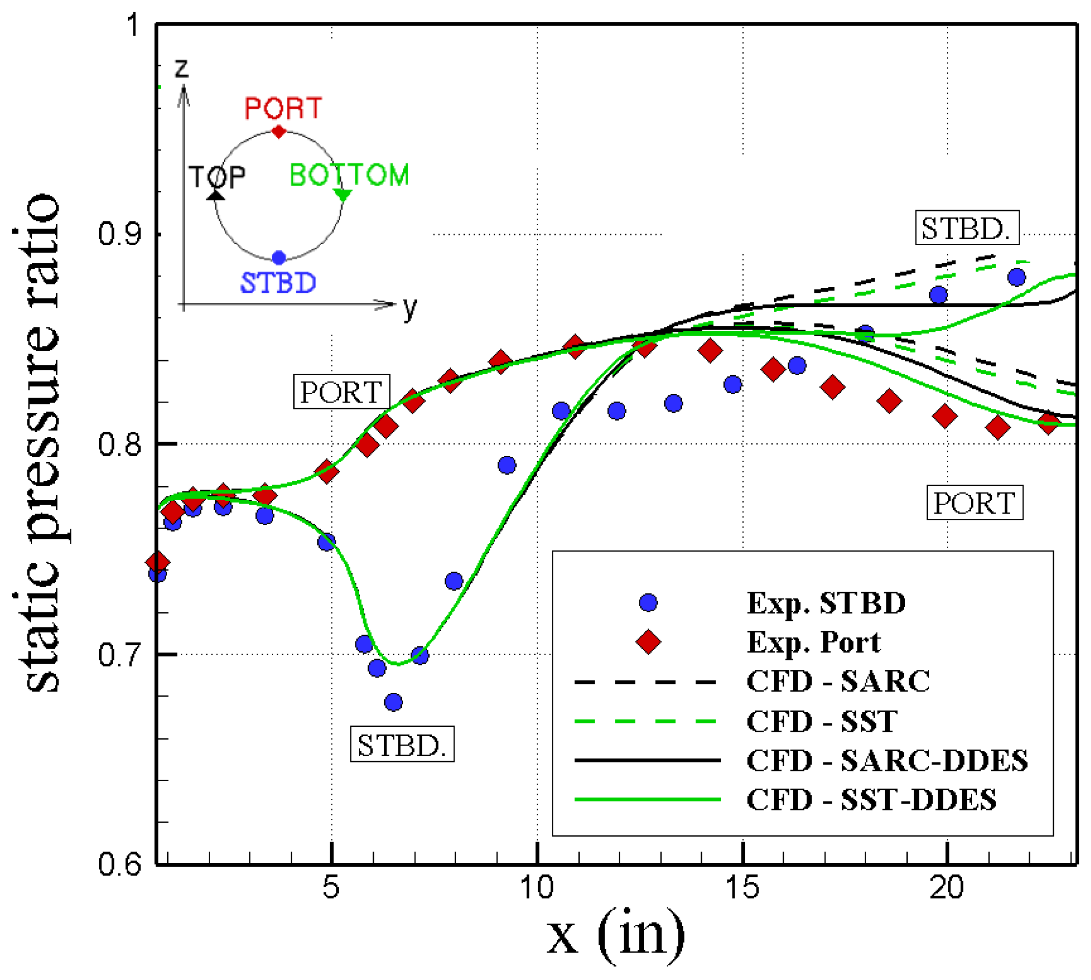
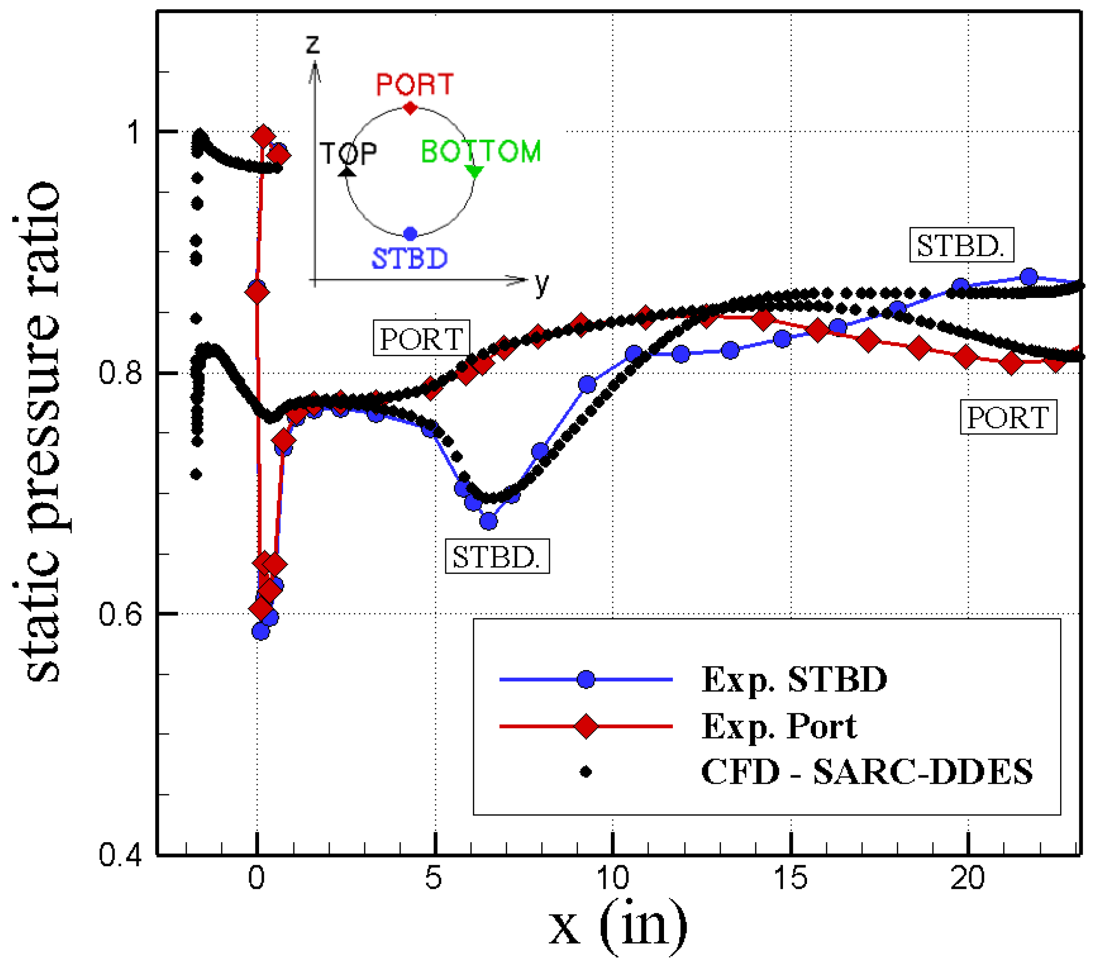
Additionally, Figure 8 compares static pressure to free-stream total pressure ratio at the port and starboard sides of the intake wall. Note that the origin was set to the most forward lip point in the experiments and the fact that CFD geometry is about 1.7 inches longer than experimental model to allow steady flow through diffuser as recommended in previous studies. Figure 8 shows that CFD data match very well with experimental data at the port side up to 14 inches. At the starboard side, measurements show flow separation at approximately $x=10.5$ inches, however, CFD predicts flow separation at further upstream distance. The starboard pressure data do not match after separation as well. At the first bend, static pressure increases (flow decelerates) at the port side and decreases (flow accelerates) at the starboard side. The diffuser flow will then decelerate at all wall sides as the diffuser cross-section increases. The flow at the port side accelerates at the second bend as well.

The effects of turbulence models on diffuser predictions are given in

Table 4. Turbulence modeling effects on the RAE-M2129 baseline predictions. NASA grid was used. CFD data are time-averaged from 2 to 2.5 s of simulation time.

	${\mathit{p}}_{0\mathit{f}}/{\mathit{p}}_{0\mathit{\infty }}$	Mach No.	${\mathit{p}}_{\mathit{f}}/{\mathit{p}}_{0\mathit{\infty }}$	DC60
Experiments	0.9744 (-)	0.4193 (-)	0.8522 (-)	0.3130 (-)
CFD–SARC + DDES	0.9776 (−0.3280%)	0.4329 (−3.243%)	0.8737 (−2.523%)	0.2945 (5.910%)
CFD–SA	0.9809 (−0.6671%)	0.4245 (−1.2402%)	0.8780 (−3.0275%)	0.2233 (28.65%)
CFD–SARC	0.9805 (−0.6260%)	0.4291 (−2.3372%)	0.8778 (−3.004%)	0.2370 (24.28%)
CFD–Menter SST	0.9790 (−0.4721%)	0.4296 (−2.4565%)	0.8770 (−2.9101%)	0.2899 (7.38%)
CFD–Menter SST + DDES	0.9778 (−0.3489%)	0.4380 (−4.4598%)	0.88715 (−4.1011%)	0.2880 (7.98%)

. Hybrid DDES models show better agreement than RANS turbulence models. SARC–DDES, in particular, has the best agreement among tested turbulence models. In more detail, Figure 9 and Figure 10 compare effects of turbulence models on the engine face and wall duct predictions. Figure 9 shows that RANS turbulence models (SA, SARC, and SST) predicted smaller distorted flow regions than hybrid DDES models and experiments. Specifically, the RANS models failed to predict the secondary vortices formed at the engine face. Additionally, SA and SARC models predict smaller primary vortices than other models and hence DC60 differences with experimental data are much larger for these models.

Figure 10 shows that all models have similar predictions up to 12 inches distance and then they become different in the separated flow region. At the port side, all models show similar trends, but hybrid DDES models match better with experimental data than RANS models. Hybrid DDES models have better agreement with experimental data at the starboard region as well. SARC and SST models do not predict any flow separation at the starboard side up to shown distance of $x=23$ inches. The air pressure at starboard side increases inside the diffuser using these RANS models. However, SARC–DDES and SST-DDES show flow separation at the starboard side at $x=14.5$ and $x=12.5$ inches, respectively. The flow is attached at further downstream distance and pressure will increase again. From these results and predictions shown in Table 4, SARC–DDES found to bring predictions closer to experiments than other models. Notice that DDES models should perform better for unsteady turbulent flows with large flow separation regions. 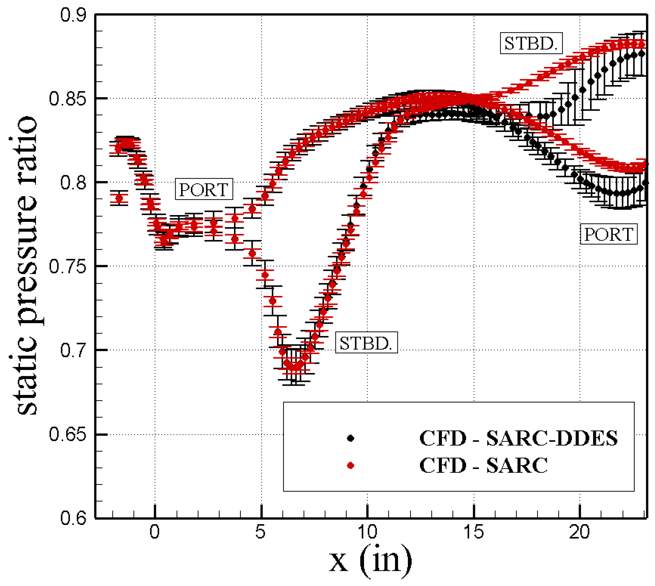In addition, Figure 11 compares SARC and SARC + DDES model predictions for port and starboard wall sides. The lines shows time-averaged data and the bars denote maximum deviation from averaged values. The results show that DDES model predicts more unsteadiness and larger variations in predictions, particularly at separated flow regions.

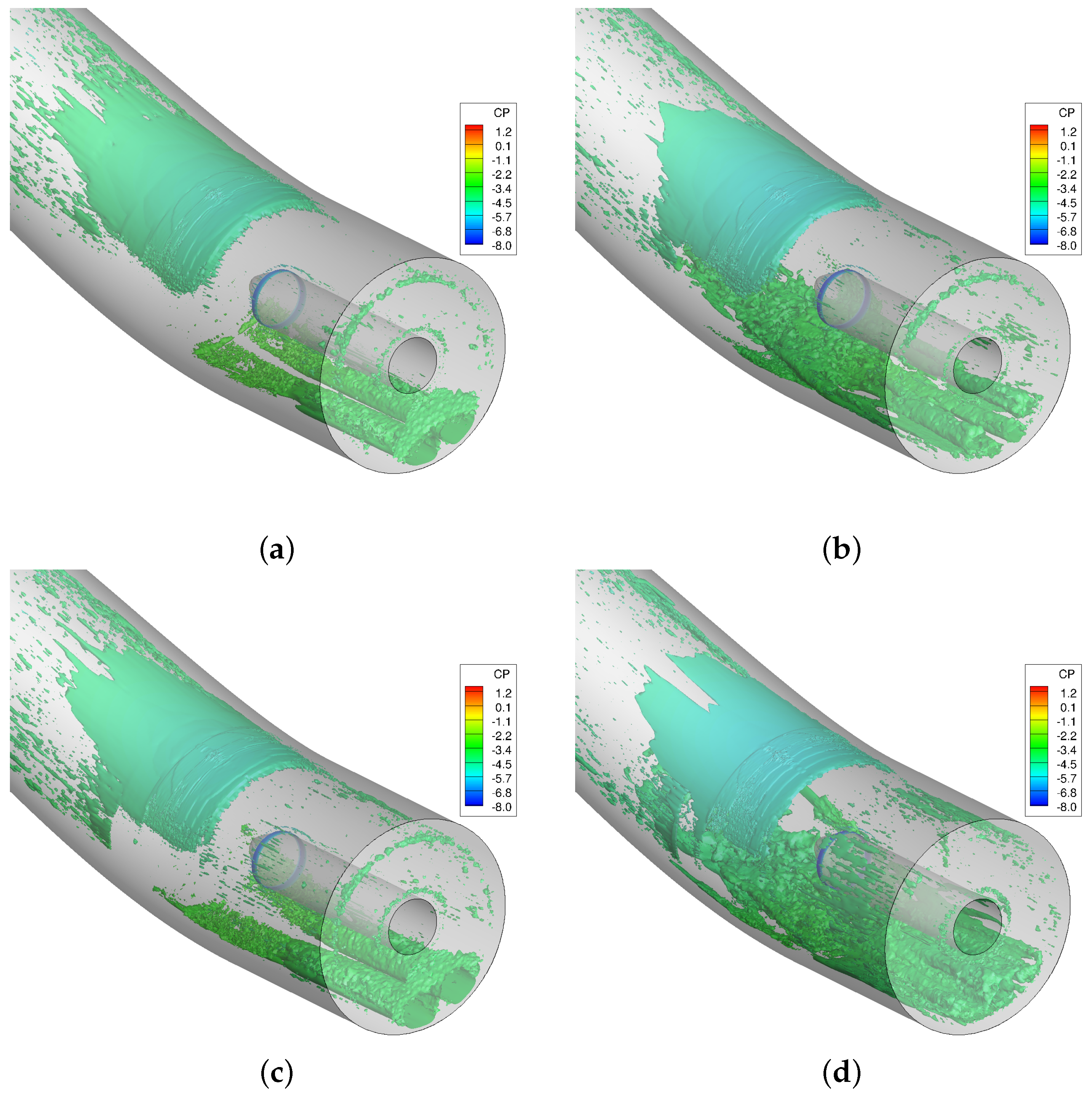
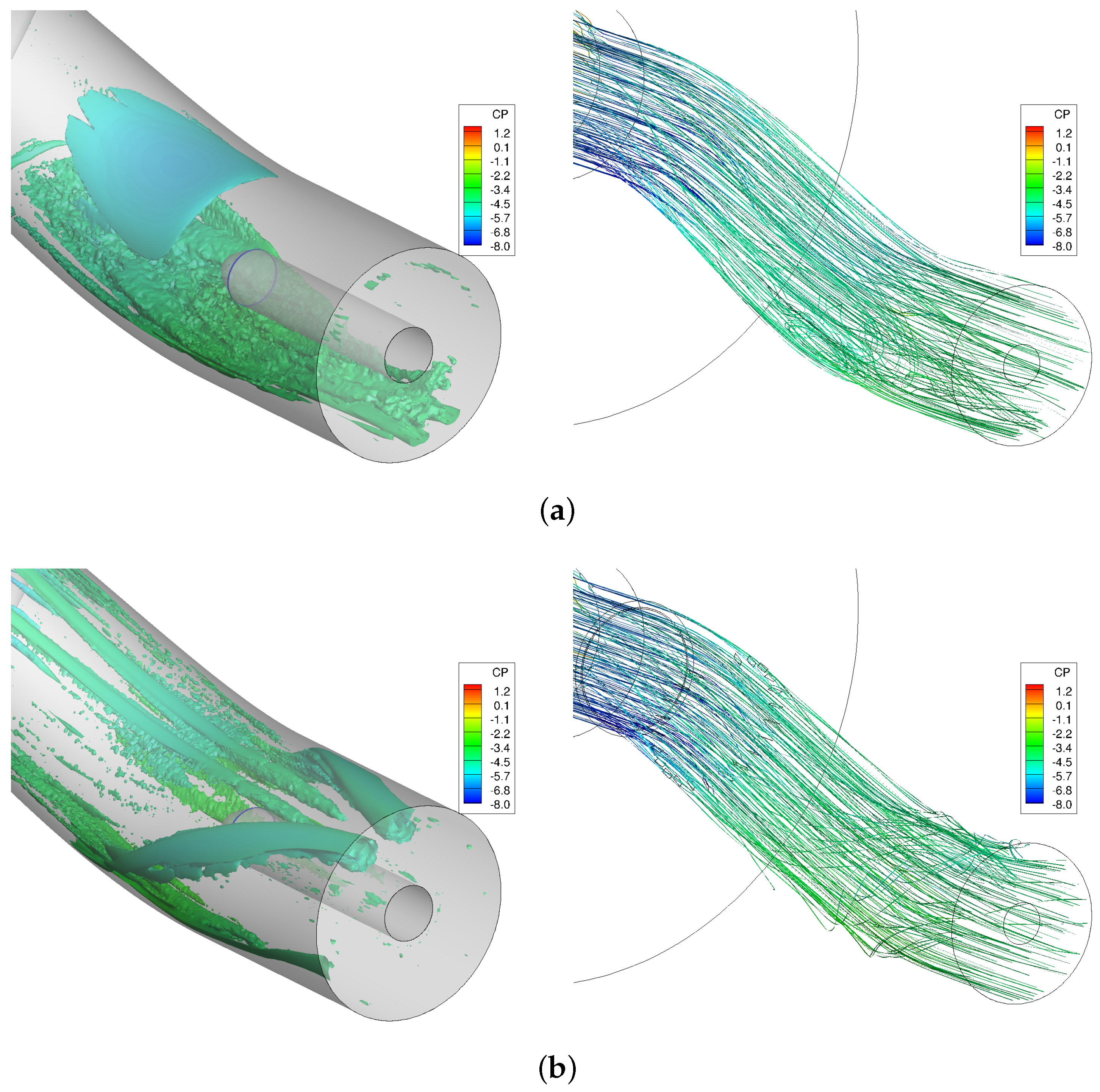
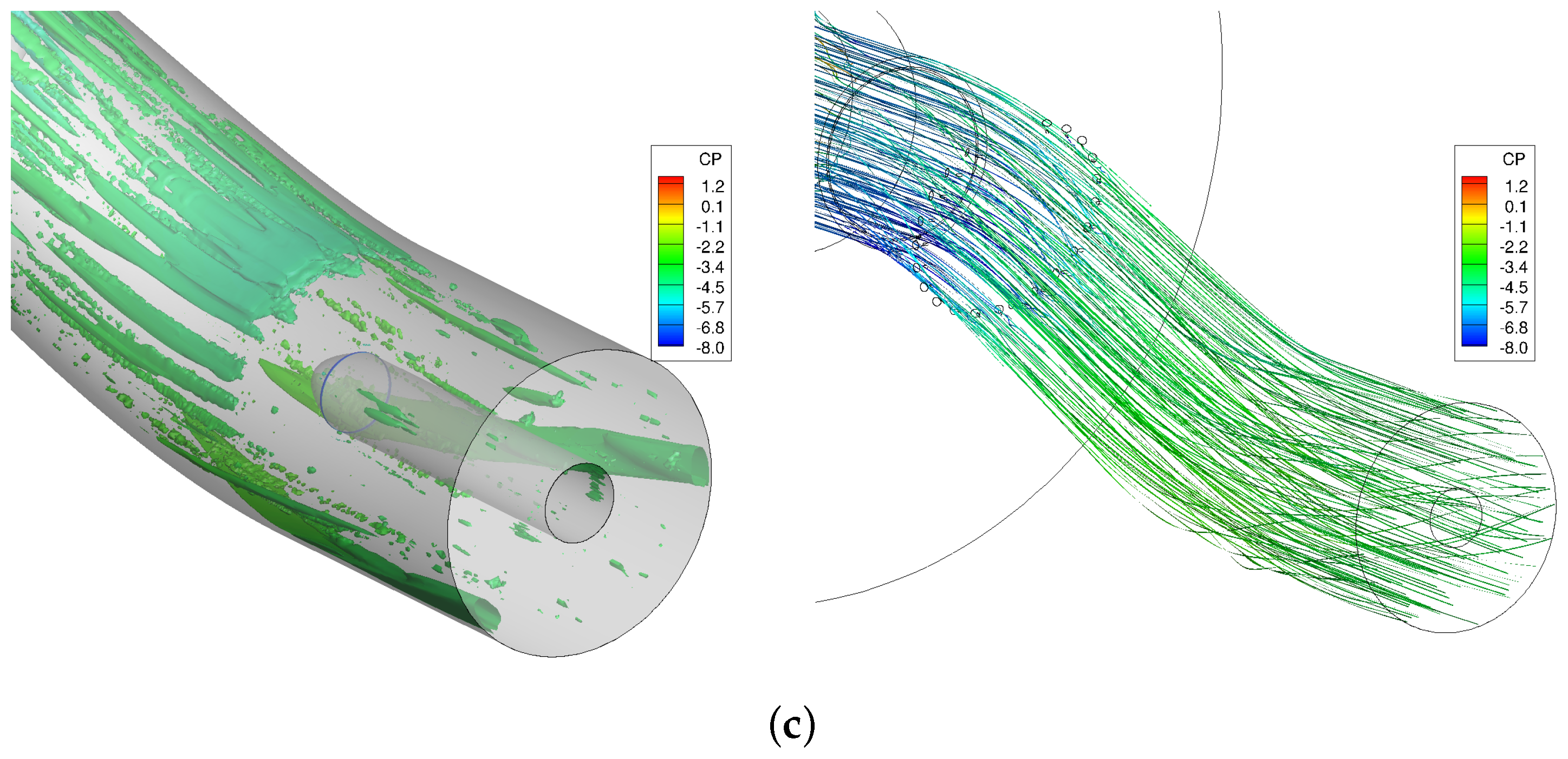
Figure 12 and Figure 13 show scaled Q (Q-criterion normalized by shear strain) isosurfaces and streamlines, respectively. These isosurfaces and streamlines are colored by pressure coefficients. Secondary and separated flow can be seen in these figures. Secondary flows are much stronger at the first bend than those formed at the second bend. Figure 12 shows that SARC and SST models predict no flow separation upstream of the bullet. These models predict primary vortices at the engine face, though SST predicted stronger vortices than SARC model. The hybrid DDES models show a flow separation region and then attachment before the bullet. Primary and secondary vortices are predicted using these turbulence models, though the strength and position of vortices are different from SARC-DDES to SST-DDES model.

Final results present the flow control simulations. The USAFA baseline grids with and without flow control are tested. The flow controls include plates and active jet vortex generators. The pressure recovery data at the engine face and symmetry plane of these configurations are shown in Figure 14. Both vortex generators reduce flow separations and first bend secondary flows and hence improve the pressure uniformity. Figure 14 shows small region of low pressure recovery at port side by using vanes. This is due to formation of secondary flows at the second bend and flow separation. Overall, the active jet flow control has better flow uniformity than vane-type method tested. In more detail,

Table 5. Flow control predictions of the RAE-M2129 intake. USAFA grids were used with SARC-DDES turbulence model. CFD data are time-averaged from 2 to 2.5 s of simulation time.

Configuration	${\mathit{p}}_{0\mathit{f}}/{\mathit{p}}_{0\mathit{\infty }}$	Mach No.	${\mathit{p}}_{\mathit{f}}/{\mathit{p}}_{0\mathit{\infty }}$	DC60
Baseline	0.97089 (-)	0.4275 (-)	0.8500 (-)	0.4215 (-)
Baseline + Vortex generators	0.97255 (0.171%)	0.4333 (1.357%)	0.8512 (0.1412%)	0.1361 (−67.7%)
Baseline + jets	0.98187 (1.131%)	0.4198 (−1.80%)	0.8675 (2.058%)	0.0881 (−79.1%)

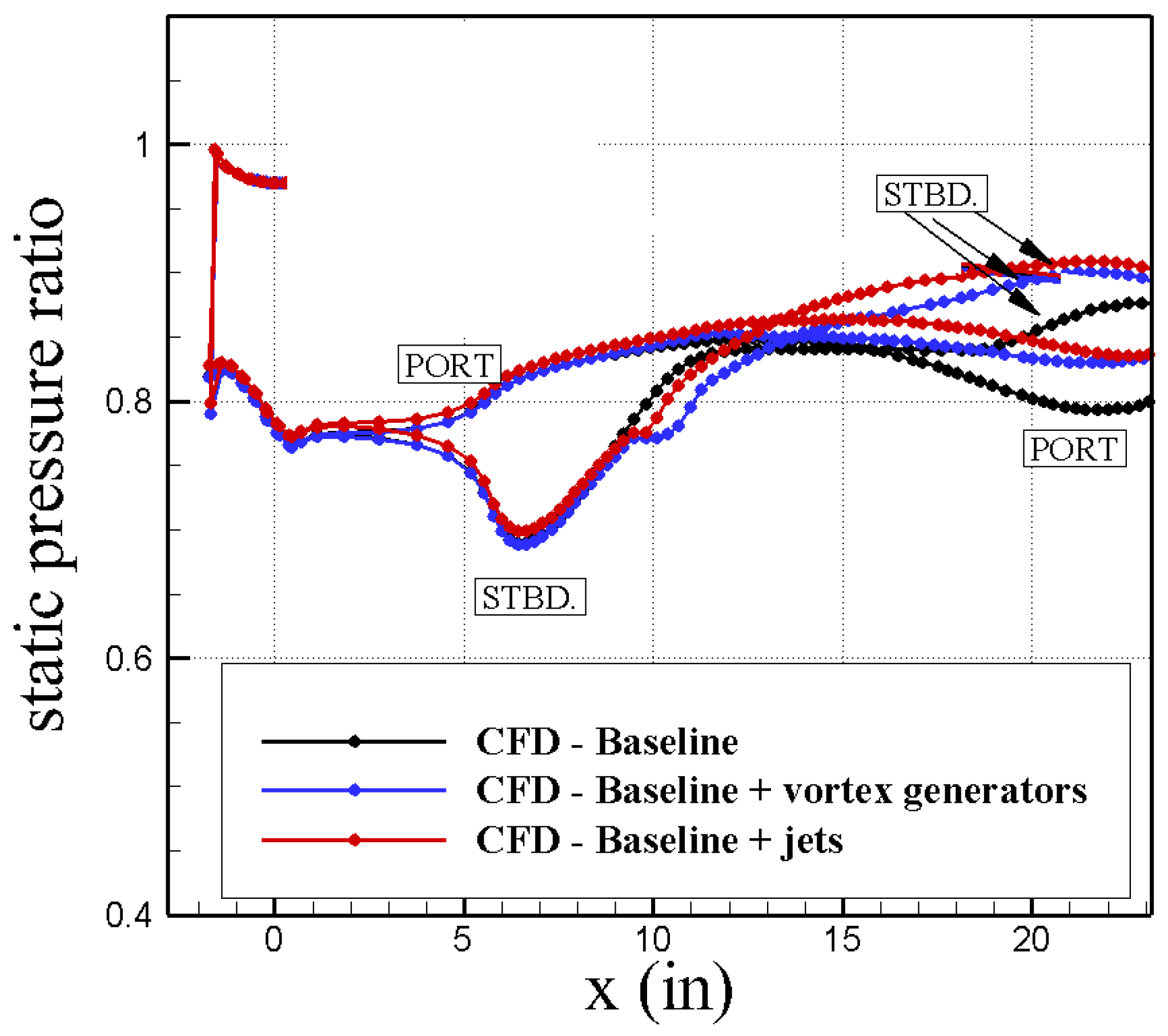
compares engine face data of these configurations. DC60 drops by 67.7% using vanes and 79.1% using jets. Pressure recovery changes are small: the jets cause the pressure recovery to increase by 1.8%. Figure 15 compares the starboard and port side static pressures of the baseline, and the baseline with vanes and jet vortex generators. Figure 15 shows that both vortex generators eliminate the flow separation region at the starboard side and at the engine face. There is a small pressure drop at about $x=9$ inches where vanes and jets are installed. The vanes cause some flow separation at the port side as well.

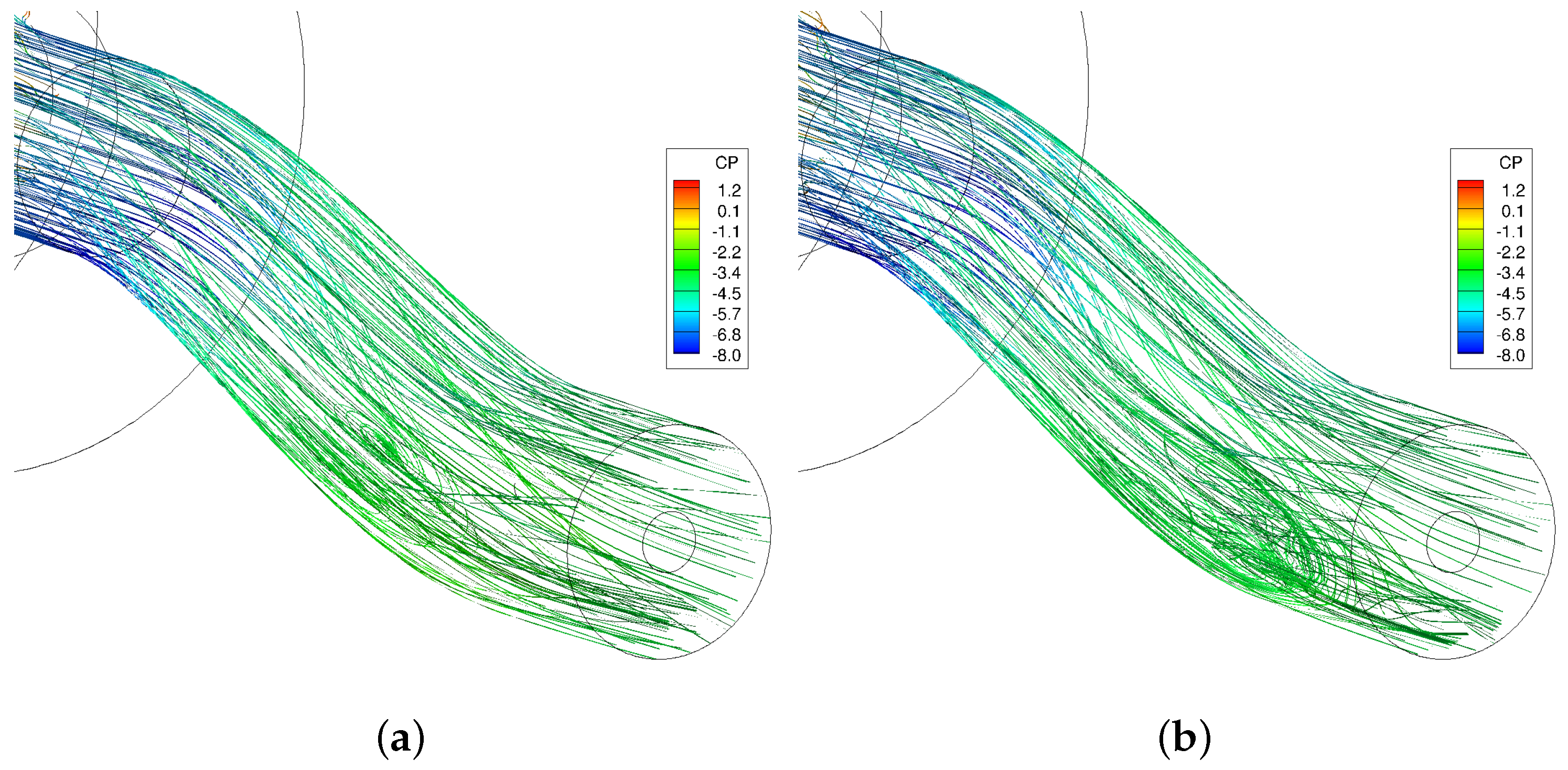
Figure 16 compares the streamlines and scaled Q isosurfaces of three configurations. Figure 16 shows that both vortex generators reduce the secondary flows at the first bend and eliminate the separation flow region at the starboard side. However, secondary flows are formed at the second bend. Vane-type vortex generators show some flow separation at the port side as well.

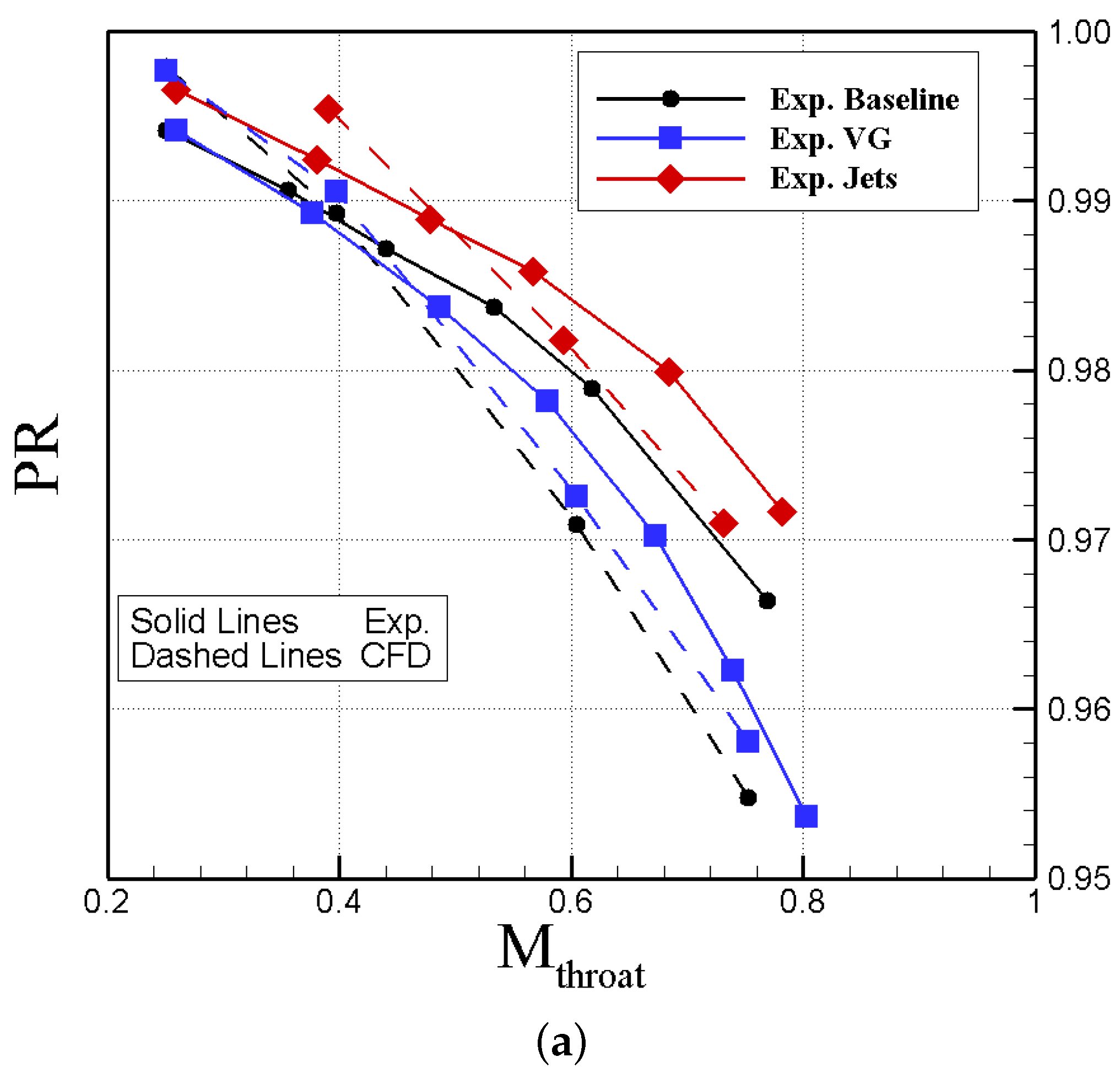
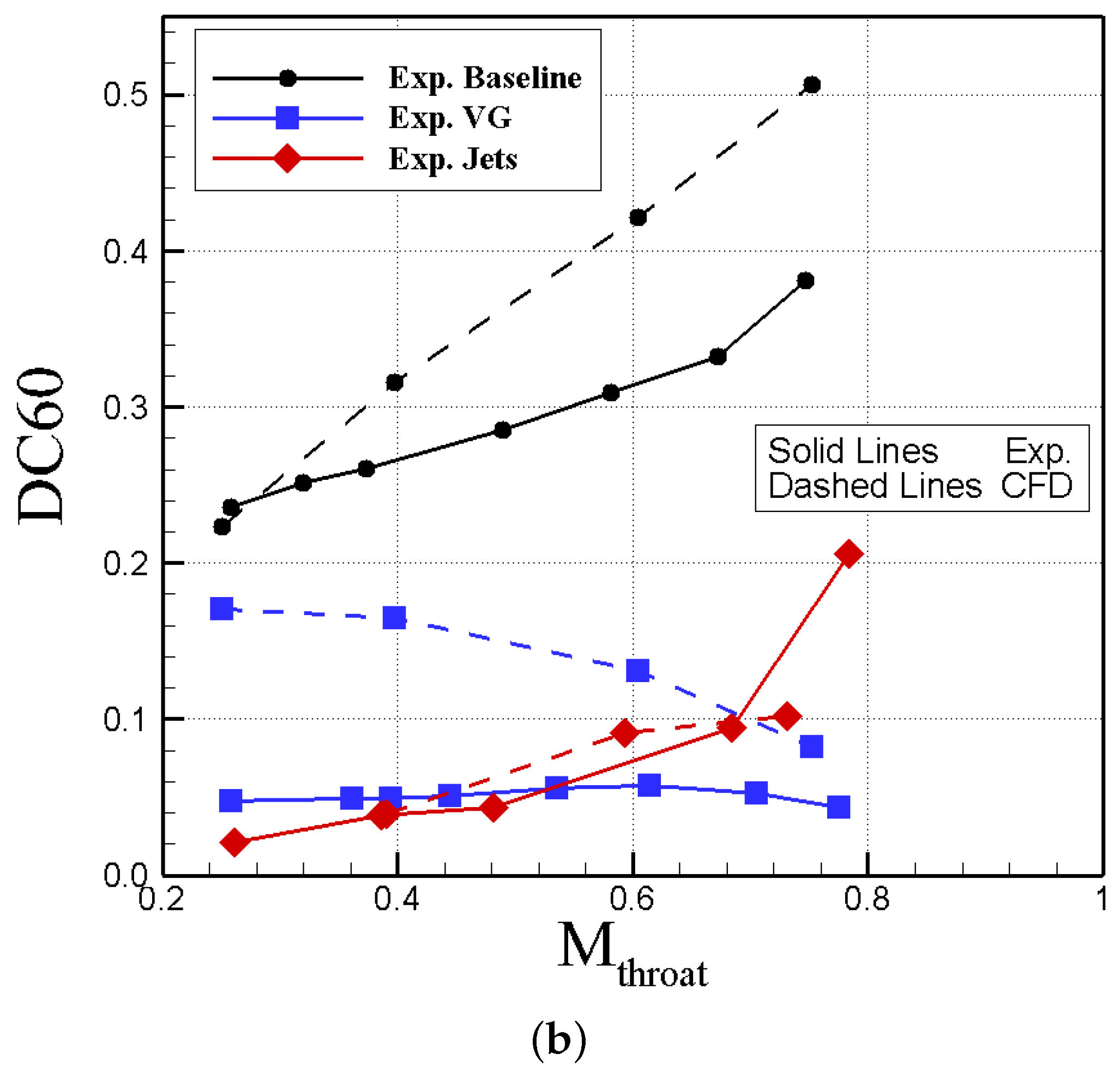
The mass flow rate through three considered ducts was adjusted such that to vary throat Mach number at the throat from 0.2 to 0.8. The predicted pressure recovery and DC60 of these ducts calculated and compared with experimental data of Ref. [12] in Figure 17. Note that baseline geometries are slightly different; the jet controls have different installation angles as well. Figure 17 shows that CFD and experiments do not match due to geometry differences, however the trend of changes are similar. Experiments shows that jets and vanes have better pressure recovery than the baseline. The pressure recovery drops by increasing throat Mach number or mass flow rate as well. CFD shows similar trends, however, the vanes of this work have lower pressure recovery values than the baseline. In addition, Figure 17b shows that jet has the smallest DC60 compared with the baseline and vanes. DC60 increases for the baseline and the baseline with jets with increasing throat Mach number. Notice that jet pressure ratio was fixed at the experiments and CFD. Predictions show similar trends for the baseline and the diffuser with jets. Both experiments and CFD show that DC60 of the diffuser with vanes slightly change with throat Mach number and even drops at larger Mach numbers.

7. Conclusions

Kestrel simulation tools were used for the validation and flow control study of RAE-M2129 intake diffuser. Two set of geometries were used: one from NASA which represent actual tested intake model and the second one a USAFA model created from intake given parameters and geometry relationships. CFD predictions of the NASA model matched well with experiments, perhaps one of the best agreements seen for this configuration and used experimental setup. All results show that there is a flow separation region at the starboard side of the intake wall with large distortion coefficients measured at the engine face. It was shown that SARC-DDES turbulence model has a better agreement compared with other tested models.

Two flow control mechanisms were investigated: (a) one using vortex generators (b) and second one using synthetic jet actuators. The results showed that both control methods reduce the distortion coefficient at the engine face. Jet vortex generators cause 79.1% drop in the flow distortion and improve the pressure recovery compared with the baseline diffuser. Vane-type vortex generators also improve the flow distortion but slightly decrease the pressure recovery values. In both control methods, secondary flows at the first bend are reduced, however both show the secondary flow at the second bend. The vanes cause the flow separate at the port side of the diffuser before the engine face. The results show that increasing the diffuser mass flow rate will cause the pressure recovery drop and the distortion coefficients to increase. The diffuser with flow control has smaller pressure recovery at diffuser conditions with larger mass flow rate. The vanes DC60, however, seems to be insensitive to mass flow rate changes and even decreases at larger values. The jets were tested at fixed bled air pressure and therefore DC60 will increase with increasing mass flow rate. However, adjusting the incoming pressure with diffuser mass flow rate can improve pressure recovery and DC60 at all tested conditions. Future work extends these results to include more flow control configuration and installation locations. The results of this work will be applied to the NATO AVT-251 muli-disciplinary configuration named Muldicon. This UCAV has a fuselage buried small turbofan engine and the intake shape design will significantly impact the engine performance.