Application of an Efficient Gradient-Based Optimization Strategy for Aircraft Wing Structures


Abstract
:
1. Introduction
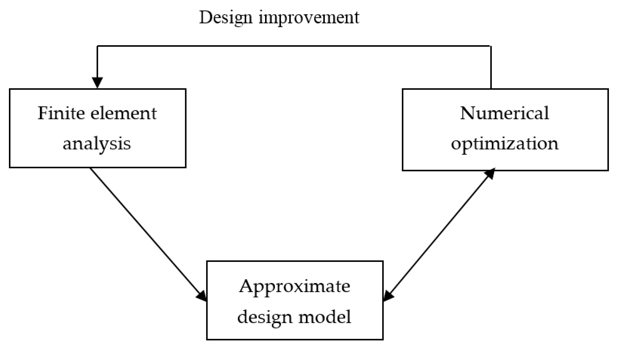
2. Realization of MSC Nastran Design Optimization Process
2.1. Design Variable Linking
2.2. Constraint Linking
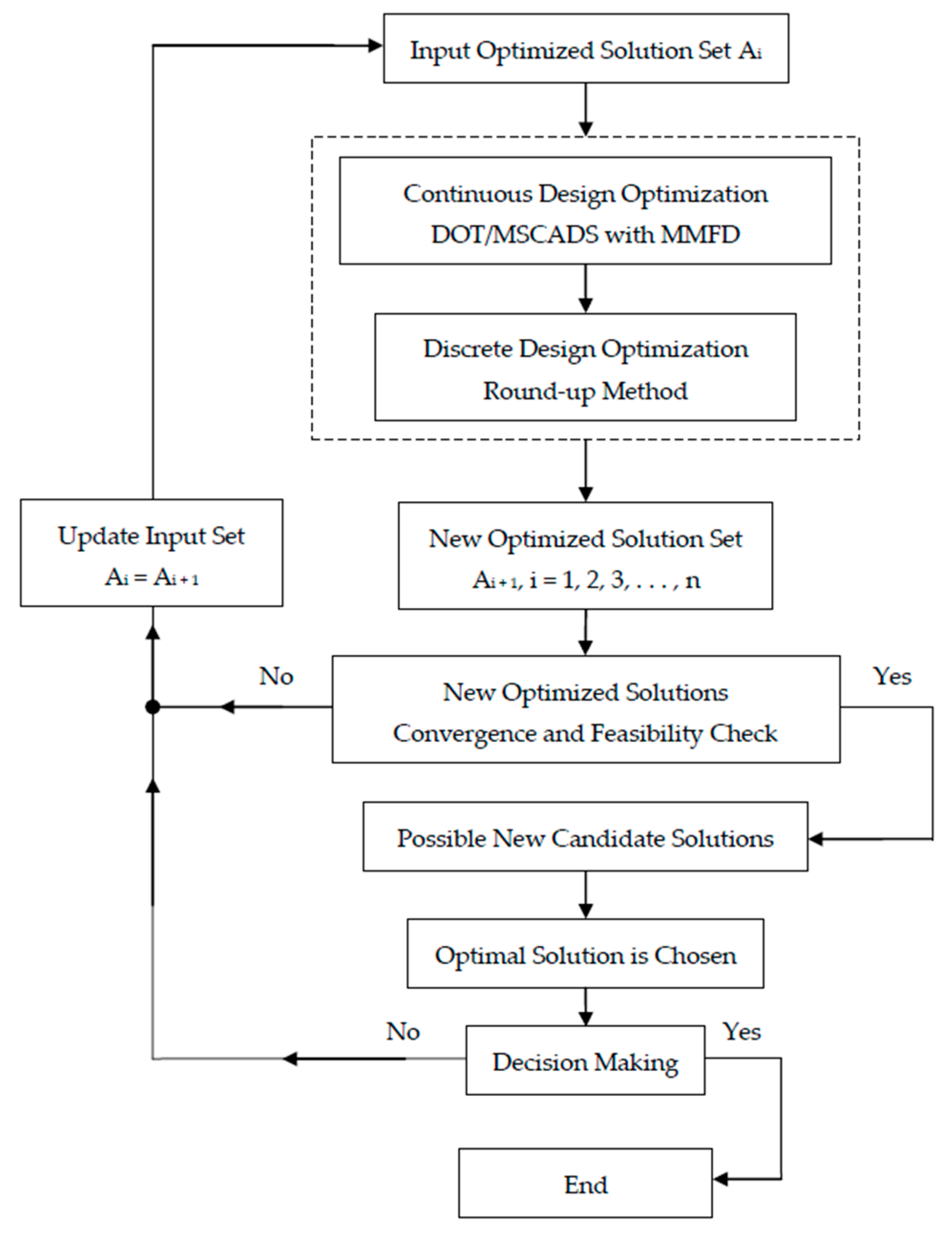
2.3. Approximate Design Model
3. Formulation of the Structural Optimization Problem
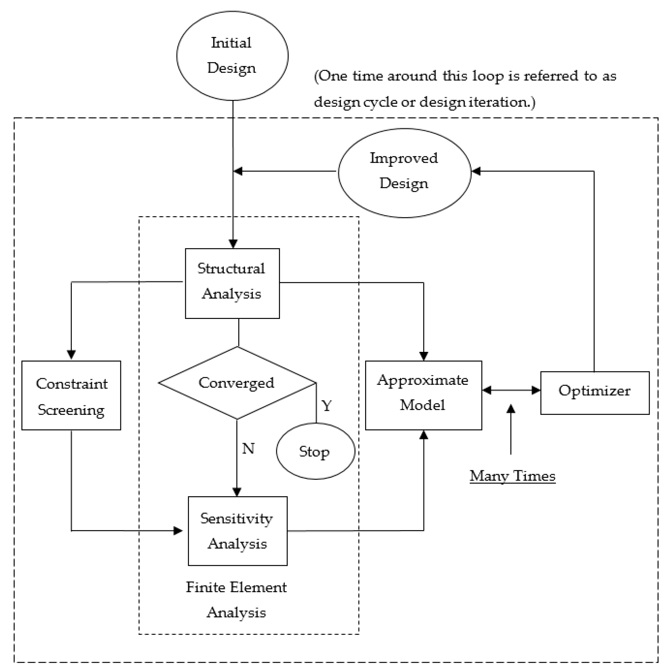
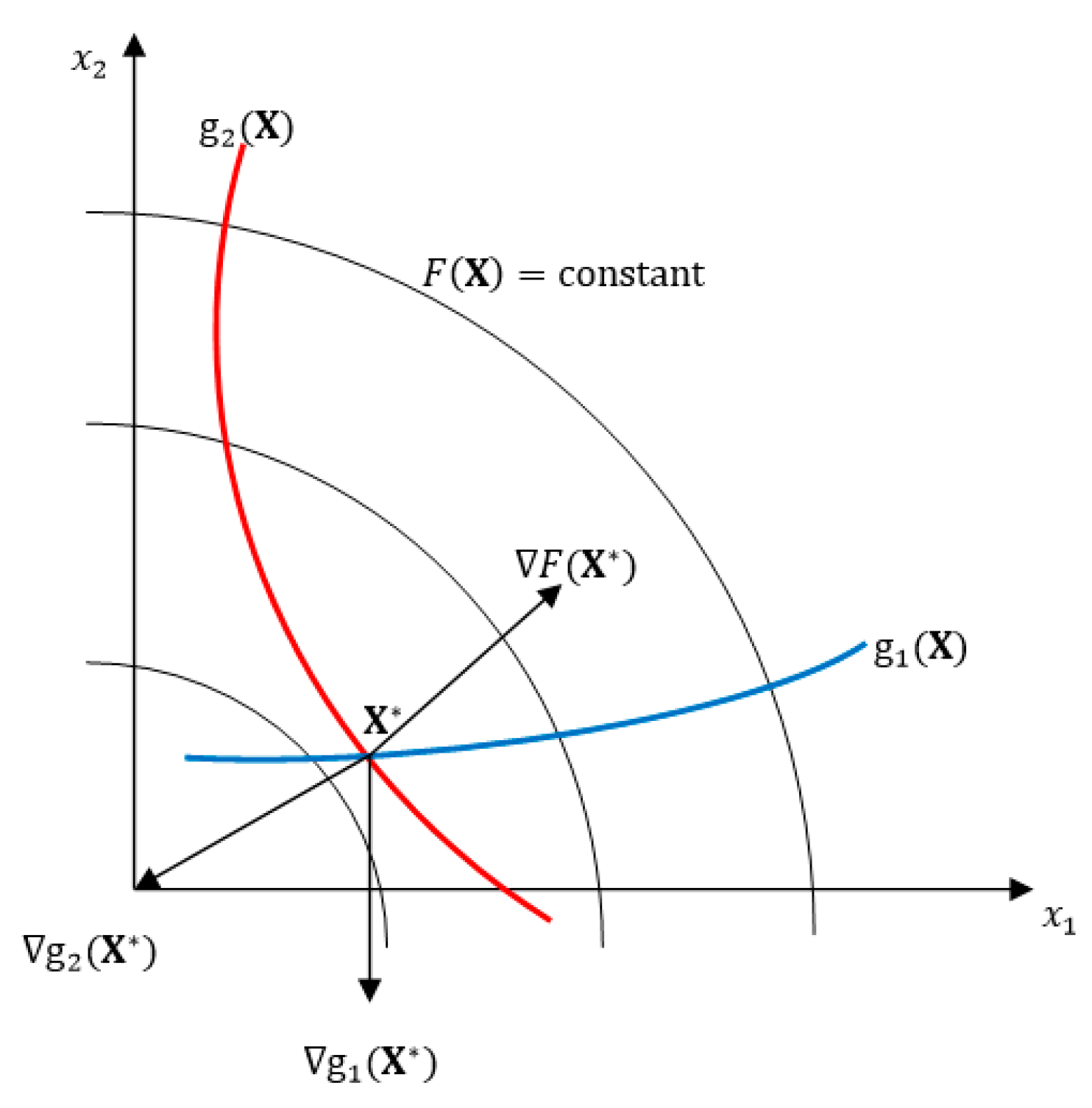
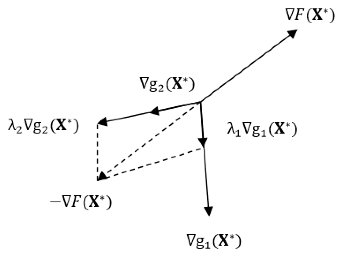
4. Gradient-Based Optimization Solution Procedure
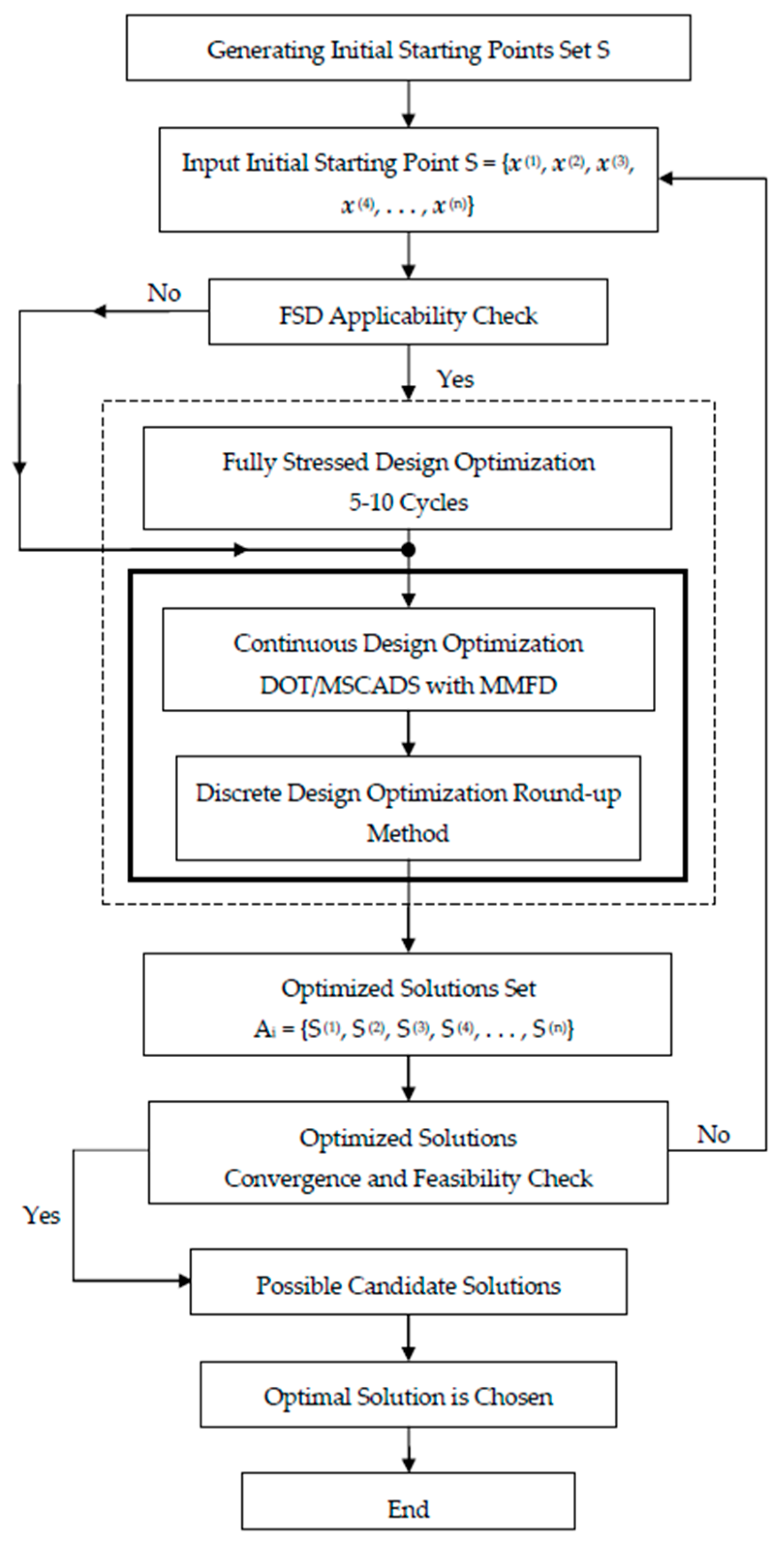
4.1. Generating Good Initial Points for the Design
- As a fraction of the upper bound value of the design variables:where is a fraction value defined by the user between , with
- Internal Halving Method:
4.2. Practical Optimization Framework
4.3. Improving the Search for the Optimum Solution
5. Structural Design Optimization Case Studies
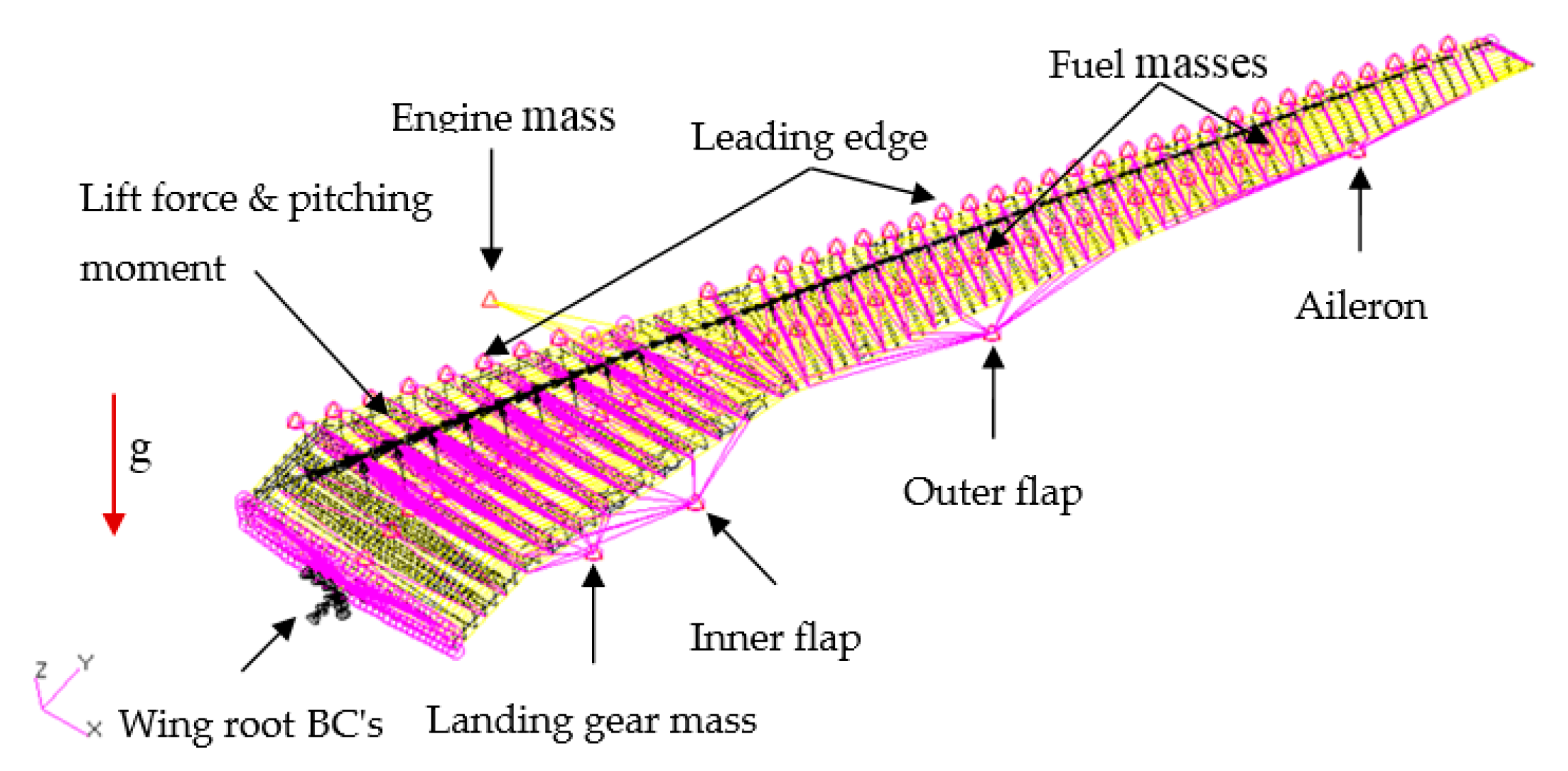
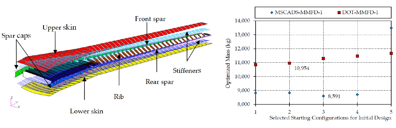
5.1. Definition of the CRM Wingbox Optimization Problem
5.1.1. Objective Function
5.1.2. Design Variables
5.1.3. Static Strength Constraints
5.1.4. Static Stiffness Constraints
5.1.5. Static Stiffness Constraints
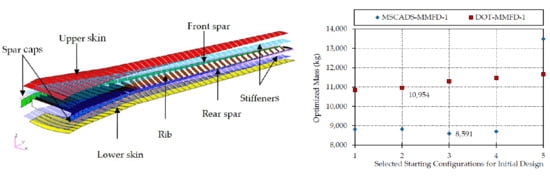
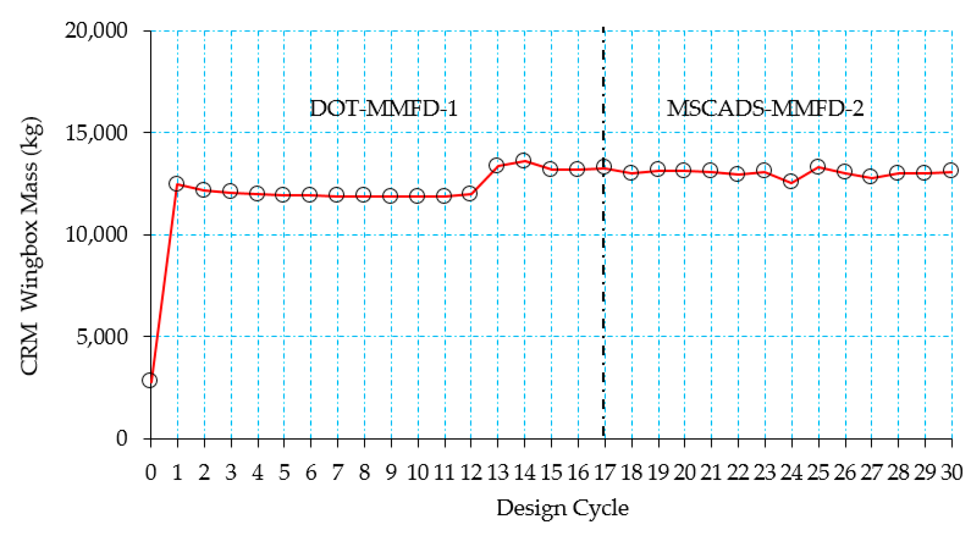
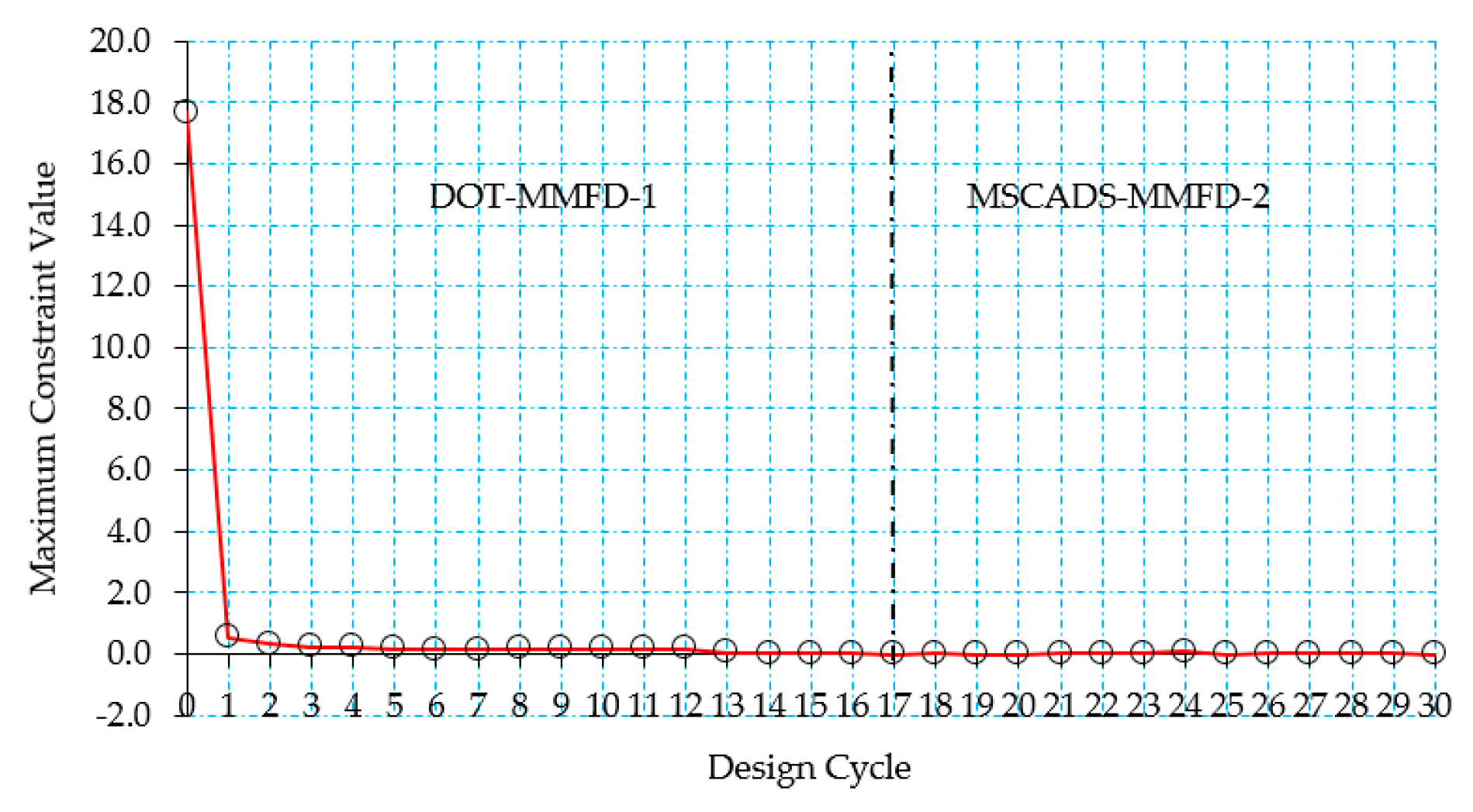
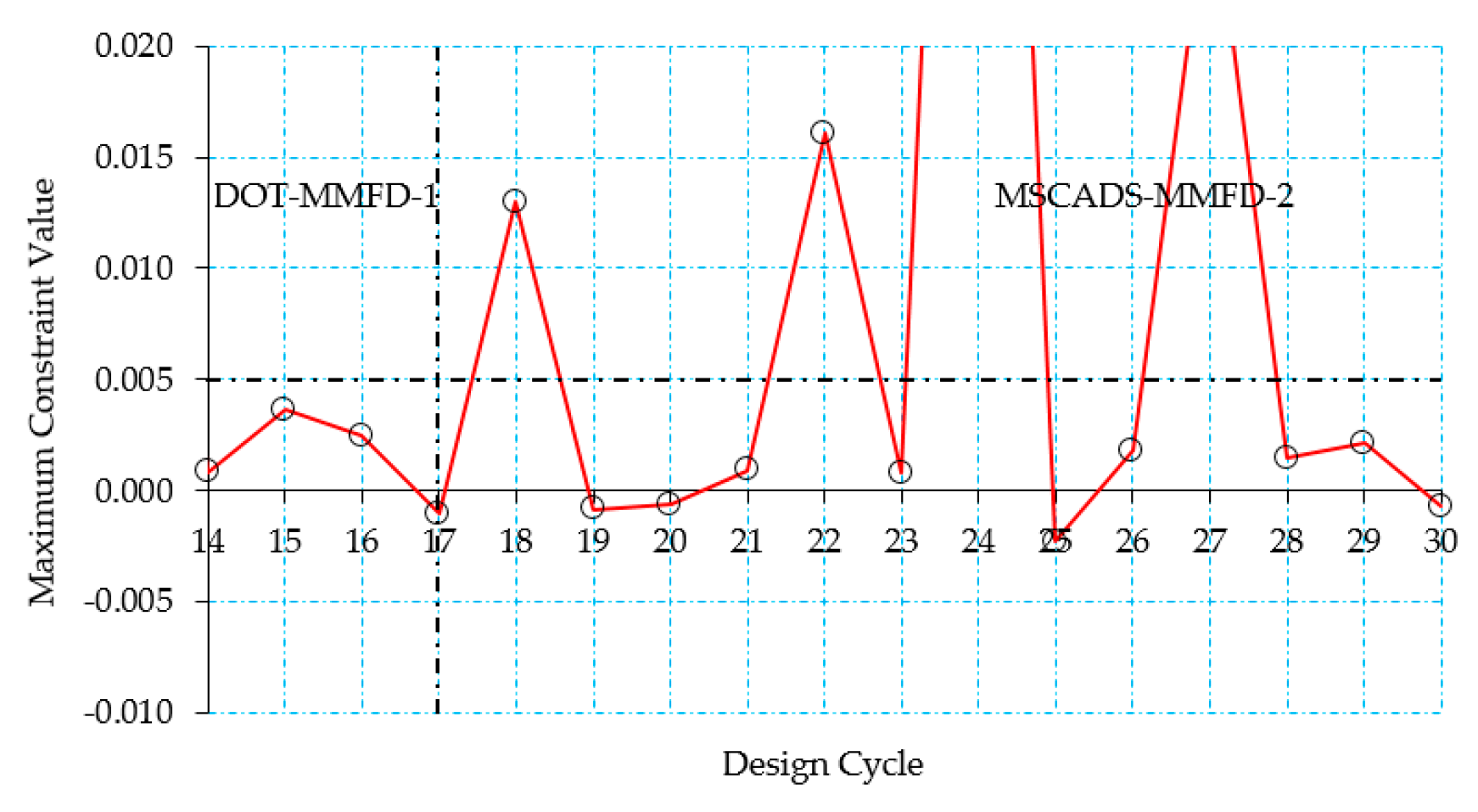
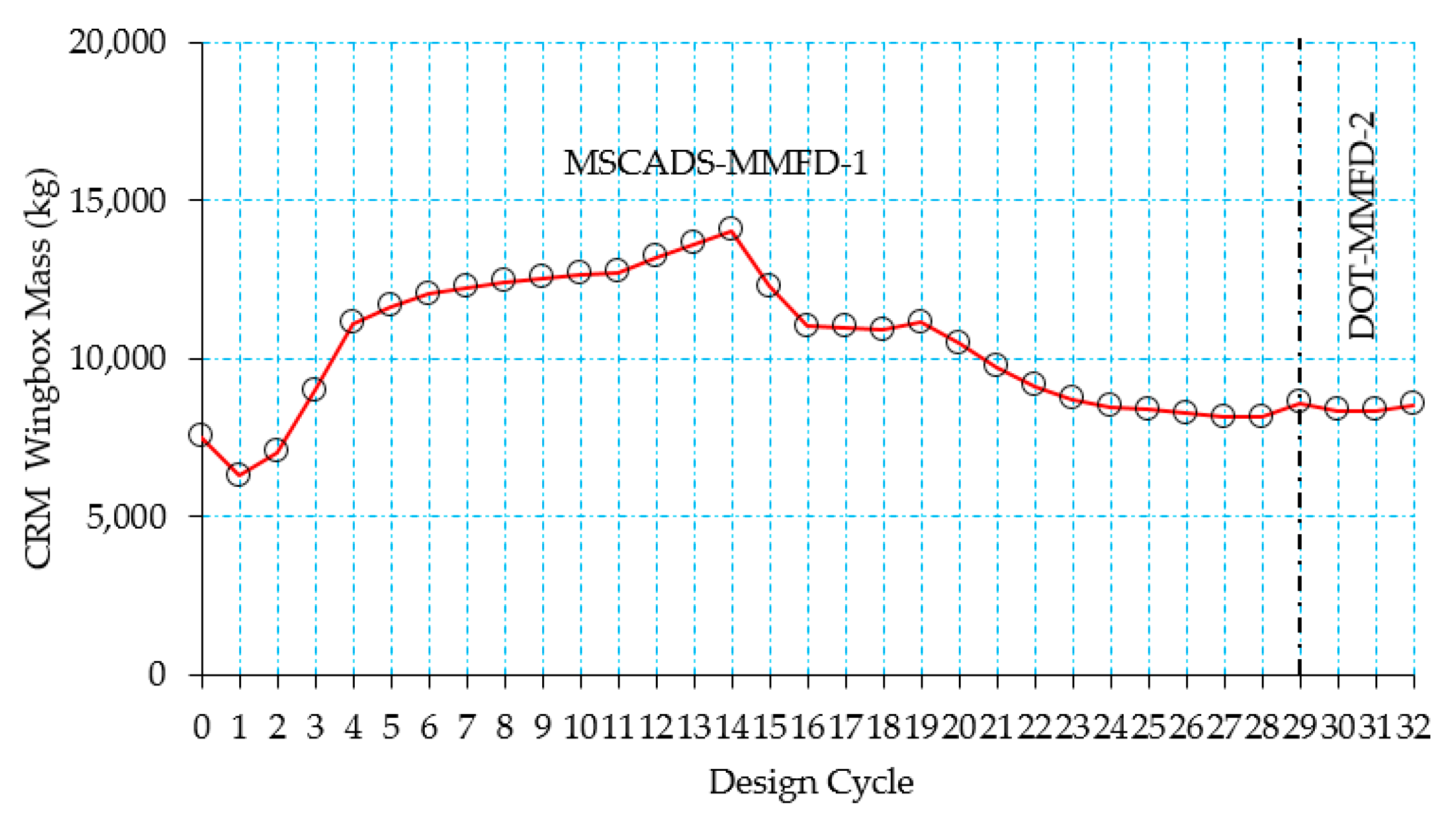
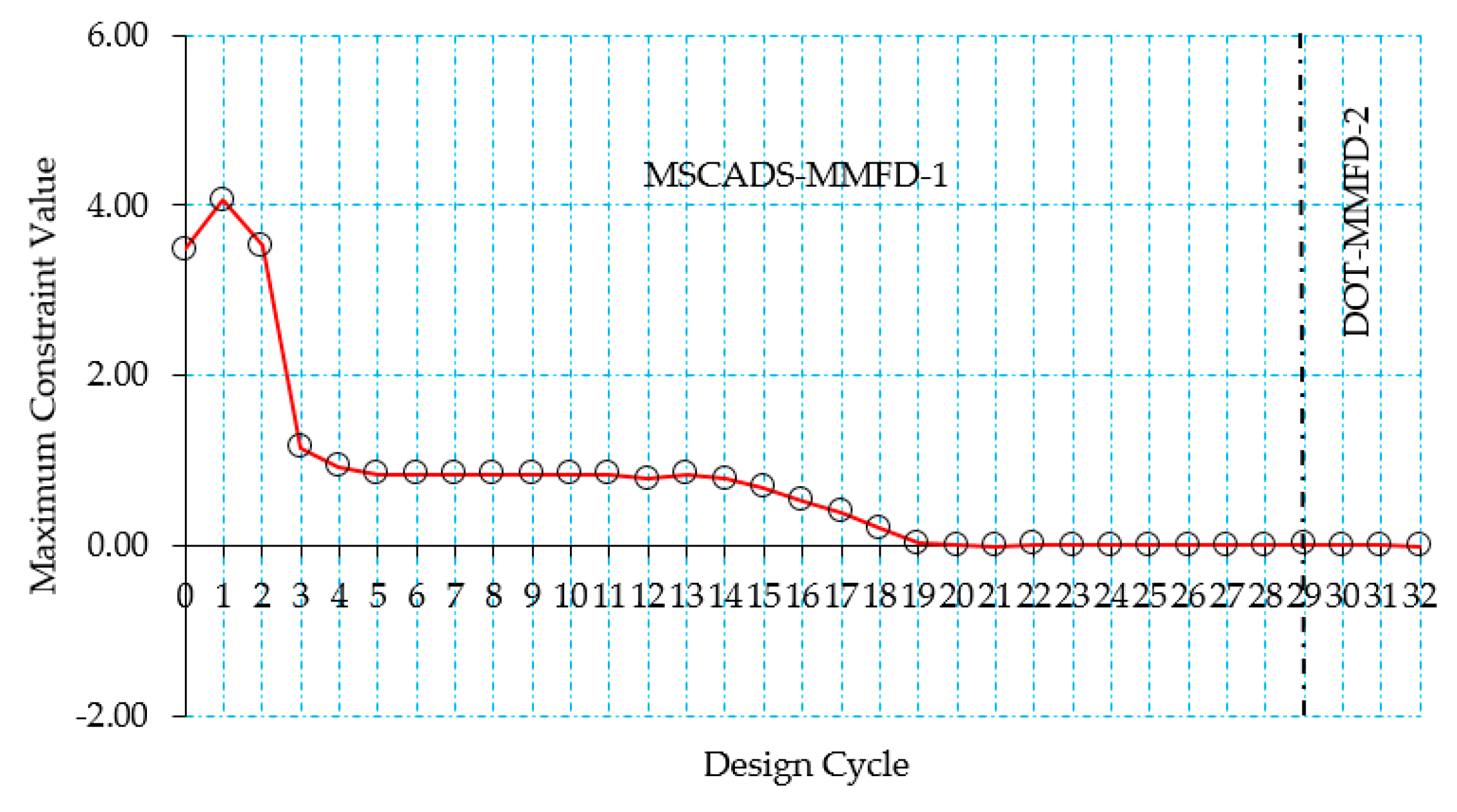
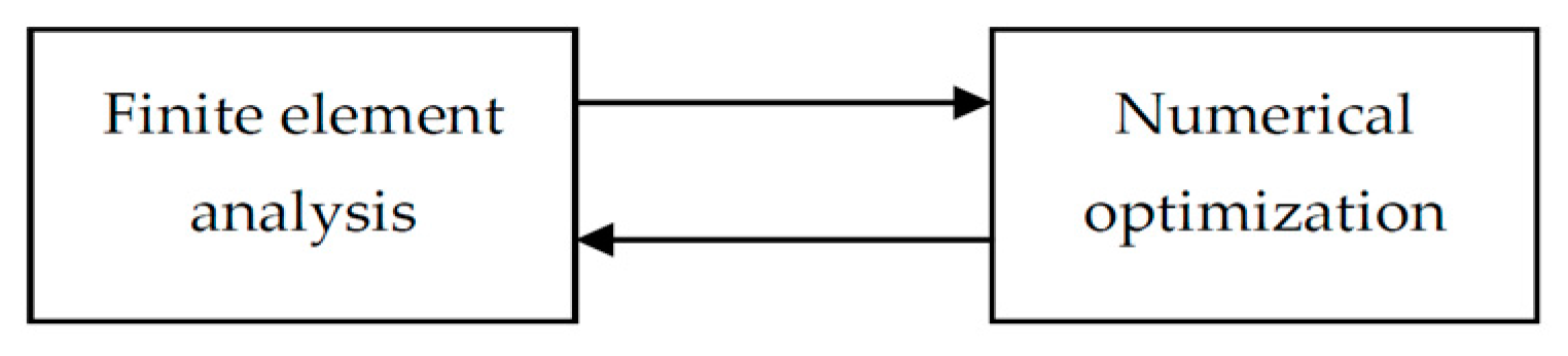
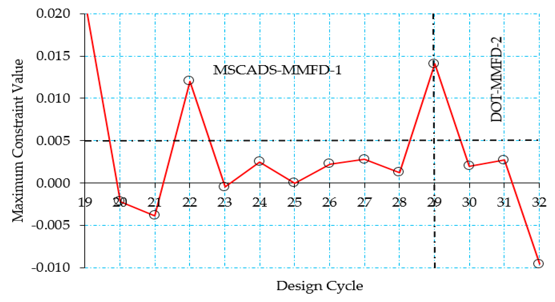
5.2. CRM Wingbox Case Studies
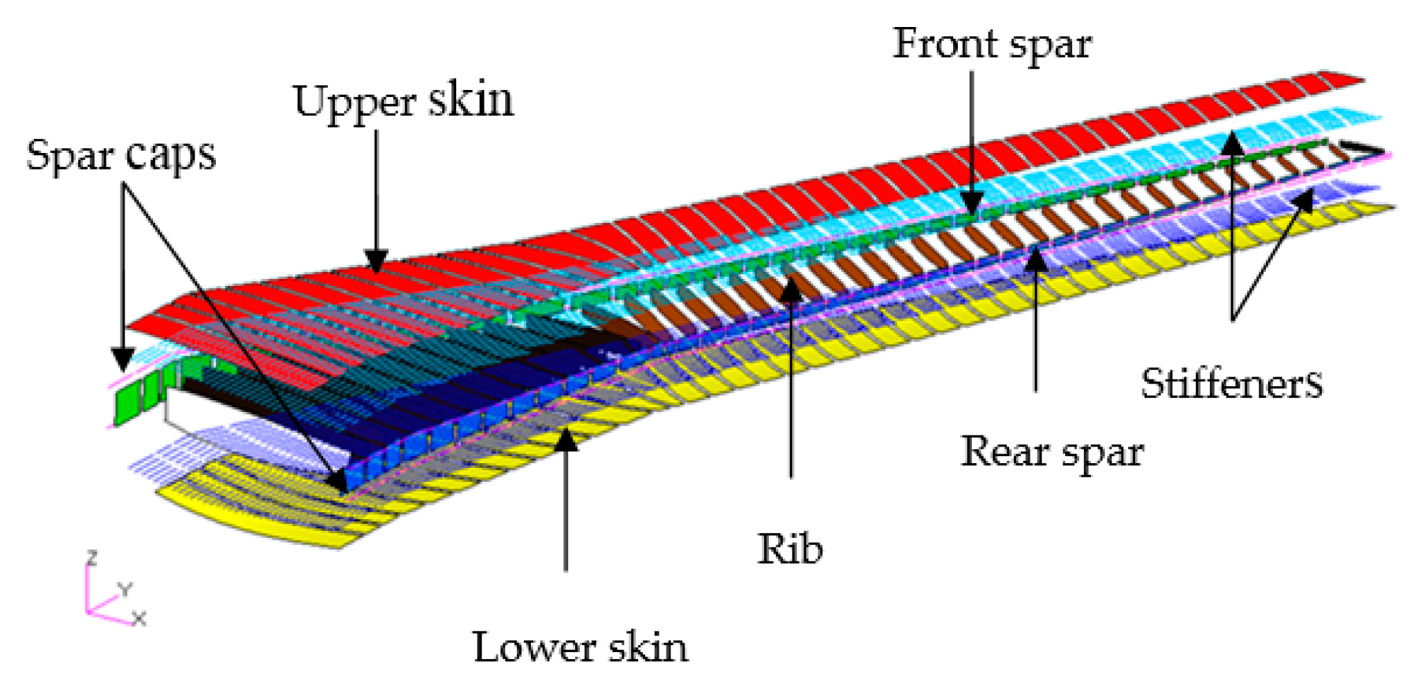
5.2.1. Metallic Wingbox Model
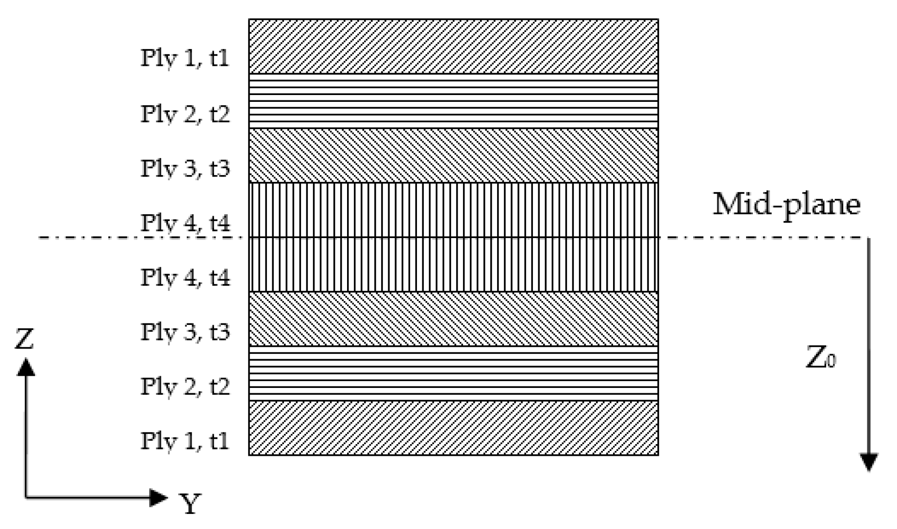
5.2.2. Composite Wingbox Model
6. Conclusions
Author Contributions
Conflicts of Interest
Appendix A.
Appendix A.1. Numerically Searching for an Optimum and Gradients Calculation


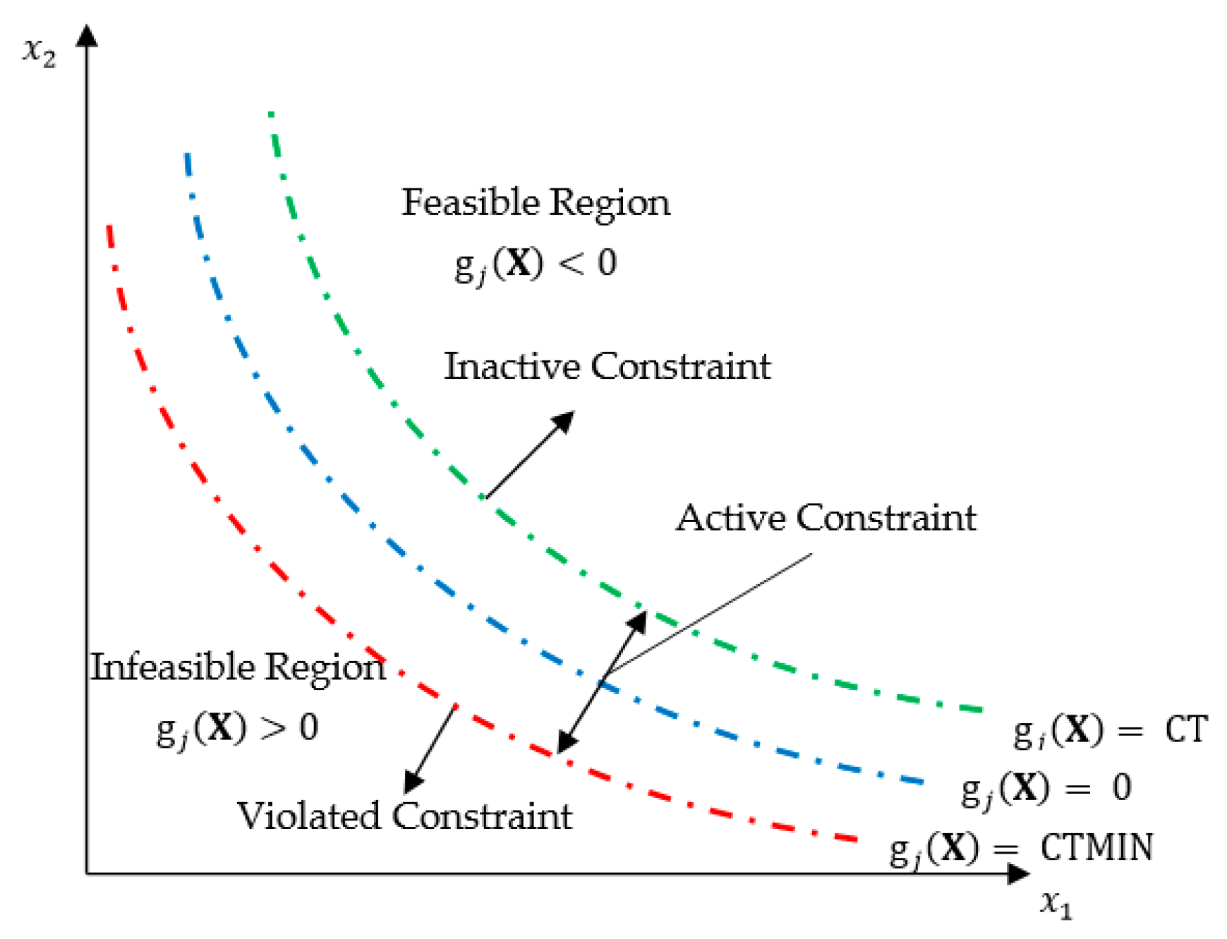
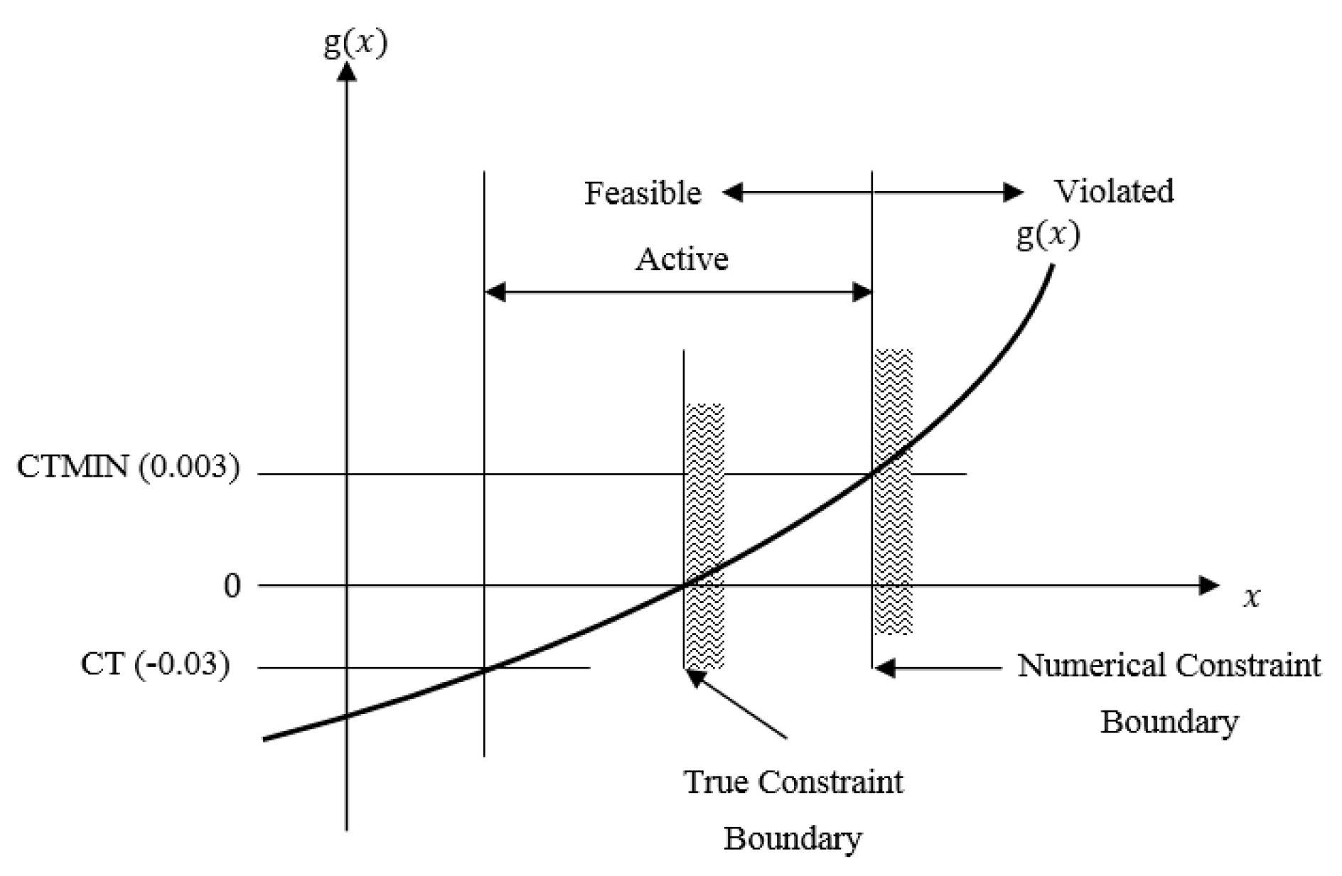
Appendix A.2. Numerically Identifying the Active and Violated Constraints

References
- Brennan, J. Integrating Optimization into the Design Process. In Proceedings of the Altair HyperWorks Technology Showcase, London, UK, 1999. [Google Scholar]
- Cervellera, P. Optimization Driven Design Process: Practical Experience on Structural Components. In Proceedings of the 14th Convegno Nazionae ADM, Bari, Italy, 31 August–2 September 2004. [Google Scholar]
- Gartmeier, O.; Dunne, W.L. Structural Optimization in Vehicle Design Development. In Proceedings of the MSC Worldwide Automotive Conference, Munich, Germany, 20–22 September 1999. [Google Scholar]
- Krog, L.; Tucker, A.; Rollema, G. Application of Topology, Sizing and Shape Optimization Methods to Optimal Design of Aircraft Components. In Proceedings of the 3rd Altair UK HyperWorks Users Conference, London, UK, 2002; Available online: http://www.soton.ac.uk/~jps7/Aircraft%20Design%20Resources/manufacturing/airbus%20wing%20rib%20design.pdf (accessed on 4 January 2018).
- Krog, L.; Tucker, A.; Kempt, M.; Boyd, R. Topology Optimization of Aircraft Wing Box Ribs, AIAA-2004-4481. In Proceedings of the 10th AIAA/ISSMO Symposium on Multidisciplinary Analysis and Optimization, Albany, NY, USA, 30 August–1 September 2004. [Google Scholar]
- Schumacher, G.; Stettner, M.; Zotemantel, R.; O’Leary, O.; Wagner, M. Optimization Assisted Structural Design of New Military Transport Aircraft, AIAA-2004-4641. In Proceedings of the 10th AIAA MAO Conference, Albany, NY, USA, 30 August–1 September 2004. [Google Scholar]
- Wasiutynski, Z.; Brandt, A. The Present State of Knowledge in the Field of Optimum Design of Structures. Appl. Mech. Rev. 1963, 16, 341–350. [Google Scholar]
- Schmit, L.A. Structural synthesis—Its genesis and development. AIAA J. 1981, 19, 1249–1263. [Google Scholar] [CrossRef]
- Vanderplaats, G.N. Structural Optimization-Past, Present, and Future. AIAA J. 1982, 20, 992–1000. [Google Scholar] [CrossRef]
- Maxwell, C. Scientific Papers. 1952, 2, 175–177. Available online: http://strangebeautiful.com/other-texts/maxwell-scientificpapers-vol-ii-dover.pdf (accessed on 21 April 2015).
- Michell, A.G. The limits of economy of material in frame-structures. Lond. Edinb. Dublin Philos. Mag. J. Sci. 1904, 8, 589–597. [Google Scholar] [CrossRef]
- Shanley, F. Weight-Strength Analysis of Aircraft Structures; Dover Publication Inc.: New York, NY, USA, 1950. [Google Scholar]
- Dantzig, G.B. Programming in Linear Structures; Comptroller, U.S.A.F: Washington, DC, USA, 1948. [Google Scholar]
- Heyman, J. Plastic Design of Beams and Frames for Minimum Material Consumption. Q. Appl. Math. 1956, 8, 373–381. [Google Scholar] [CrossRef]
- Schmit, L.A. Structural Design by Systematic Synthesis. In Proceedings of the 2nd Conference ASCE on Electronic Computation, Pittsburgh, PA, USA, 8–10 September 1960; American Society of Civil Engineers: Reston, VA, USA, 1960; pp. 105–122. [Google Scholar]
- Venkayya, V.B. Design of Optimum Structures. Comput. Struct. 1971, 1, 265–309. [Google Scholar] [CrossRef]
- Prager, W.; Taylor, J.E. Problems in Optimal Structural Design. J. Appl. Mech. 1968, 36, 102–106. [Google Scholar] [CrossRef]
- Schmit, L.A.; Farshi, B. Some Approximation Concepts for Structural Synthesis. AIAA J. 1974, 12, 692–699. [Google Scholar] [CrossRef]
- Starnes, J.R., Jr.; Haftka, R.T. Preliminary Design of Composite Wings for Buckling, Stress and Displacement Constraints. J. Aircr. 1979, 16, 564–570. [Google Scholar] [CrossRef]
- Gellatly, R.H.; Berke, L.; Gibson, W. The use of Optimality Criterion in Automated Structural Design. In Proceedings of the 3rd Air Force Conference on Matrix Methods in Structural Mechanics, Wright Patterson AFB, OH, USA, 19–21 October 1971. [Google Scholar]
- Brugh, R.L. NASA Structural Analysis System (NASTRAN); National Aeronautics and Space Administration (NASA): Washington, DC, USA, 1989.
- Haug, E.J.; Choi, K.K.; Komkov, V. Design Sensitivity Analysis of Structural Systems, 1st ed.; Academic Press: Cambridge, MA, USA, 1986; Volume 177. [Google Scholar]
- Haftka, R.T.; Adelman, H.M. Recent developments in structural sensitivity analysis. Struct. Optim. 1989, 1, 137–151. [Google Scholar] [CrossRef]
- Arora, J.S.; Huang, M.W.; Hsieh, C.C. Methods for optimization of nonlinear problems with discrete variables: A review. Struct. Optim. 1994, 8, 69–85. [Google Scholar] [CrossRef]
- Sandgren, E. Nonlinear integer and discrete programming for topological decision making in engineering design. J. Mech. Des. 1990, 112, 118–122. [Google Scholar] [CrossRef]
- Thanedar, P.B.; Vanderplaats, G.N. Survey of Discrete Variable Optimization for Structural Design. J. Struct. Eng. ASCE 1995, 121, 301–306. [Google Scholar] [CrossRef]
- Moore, G.J. MSC Nastran 2012 Design Sensitivity and Optimization User’s Guide; MSC Software Corporation: Santa Ana, CA, USA, 2012. [Google Scholar]
- Gill, P.; Murray, W.; Saunders, M. SNOPT: An SQP Algorithm for Large Scale Constrained Optimization. SIAM J. Optim. 2002, 12, 979–1006. [Google Scholar] [CrossRef]
- Dennis, J.E., Jr.; Schnabel, R.B. Numerical Methods for Unconstrained Optimization and Nonlinear Equations; Prentice Hall: Englewood Cliffs, NJ, USA, 1983. [Google Scholar]
- Kim, H.; Papila, M.; Mason, W.H.; Haftka, R.T.; Watson, L.T.; Grossman, B. Detection and Repair of Poorly Converged Optimization Runs. AIAA J. 2001, 39, 2242–2249. [Google Scholar] [CrossRef]
- Klimmek, T. Parametric Set-Up of a Structural Model for FERMAT Configuration for Aeroelastic and Loads Analysis. J. Aeroelast. Struct. Dyn. 2014, 3, 31–49. [Google Scholar]
- Jutte, C.V.; Stanford, B.K.; Wieseman, C.D. Internal Structural Design of the Common Research Model Wing Box for Aeroelastic Tailoring; Technical Report-TM-2015-218697; National Aeronautics and Space Administration (NASA): Hampton, VA, USA, 2015.
- Federal Aviation Administration (FAA). FAR 25, Airworthiness Standards: Transport Category Airplanes (Title 14 CFR Part 25). Available online: http://flightsimaviation.com/data/FARS/part_25.html (accessed on 15 January 2014).
- European Aviation Safety Agency (EASA). Certification Specifications and Acceptable Means of Compliance for Large Aeroplanes CS-25, Amendment 16. Available online: http://easa.europa.eu/system/files/dfu/CS-25 20Amdendment 16.pdf (accessed on 28 March 2015).
- ESDU. Computer Program for Estimation of Spanwise Loading of Wings with Camber and Twist in Subsonic Attached Flow. Lifting-Surface Theory. 1999. Available online: https://www.esdu.com/cgi-bin/ps.pl?sess=cranfield5_1160220142018cql&t=doc&p=esdu_95010c (accessed on 12 March 2014).
- Tomas, M. User’s Guide and Reference Manual for Tornado. 2000. Available online: http://www.tornado.redhammer.se/index.php/documentation/documents (accessed on 12 March 2014).
- Torenbeek, E. Development and Application of a Comprehensive Design Sensitive Weight Prediction Method for Wing Structures of Transport Category Aircraft; Delft University of Technology: Delft, The Netherlands, 1992. [Google Scholar]
- Jones, R.M. Mechanics of Composite Materials, 2nd ed.; Taylor & Francis: New York, NY, USA, 1999. [Google Scholar]
- Tsai, S.W.; Hahn, H.T. Introduction to Composite Materials; Technomic Publishing Co.: Lancaster, PA, USA, 1980. [Google Scholar]
- Kassapoglou, C. Review of Laminate Strength and Failure Criteria, in Design and Analysis of Composite Structures: with Applications to Aerospace Structures; John Wiley & Sons Ltd.: Oxford, UK, 2013. [Google Scholar]
- Niu, M.C. Composite Airframe Structures, 3rd ed.; Conmilit Press Ltd.: Hong Kong, China, 2010. [Google Scholar]
- Oliver, M.; climent, H.; Rosich, F. Non Linear Effects of Applied Loads and Large Deformations on Aircraft Normal Modes. In Proceedings of the RTO AVT Specialists’ Meeting on Structural Aspects of Flexible Aircraft Control, Ottawa, ON, Canada, 18–20 October 1999. [Google Scholar]
- Liu, Q.; Mulani, S.; Kapani, R.K. Global/Local Multidisciplinary Design Optimization of Subsonic Wing, AIAA 2014-0471. In Proceedings of the 10th AIAA Multidisciplinary Design Optimization Conference, National Harbor, MD, USA, 13–17 January 2014. [Google Scholar]
- Barker, D.K.; Johnson, J.C.; Johnson, E.H.; Layfield, D.P. Integration of External Design Criteria with MSC. Nastran Structural Analysis and Optimization. In Proceedings of the MSC Worldwide Aerospace Conference & Technology Showcase, Toulouse, France, 24–16 September 2001; MSC Software Corporation: Santa Ana, CA, USA, 2002. [Google Scholar]
- ASM Aerospace Specification Metals Inc. (ASM). ASM Aerospace Specification Metals, Aluminum 7050-T7451. 1978. Available online: http://asm.matweb.com/search/SpecificMaterial.asp?bassnum=MA7050T745 (accessed on 12 June 2014).
- ASM Aerospace Specification Metals Inc. (ASM). ASM Aerospace Specification Metals, Aluminum 2024-T3. 1978. Available online: http://asm.matweb.com/search/SpecificMaterial.asp?bassnum=%20MA2024T3 (accessed on 12 June 2014).
- Soni, S.R. Elastic Properties of T300/5208 Bidirectional Symmetric Laminates—Technical Report Afwal-Tr-80-4111; Materials Laboratory, Air Force Wright Aeronautical Laboratories, Air Force Systems Command: Dayton, OH, USA, 1980. [Google Scholar]
- MSC Patran Laminate Modeler User’s Guide; MSC Software Corporation: Santa Ana, CA, USA, 2008.


| Description | Value |
|---|---|
| Maximum take-off mass | 260,000 kg |
| Maximum zero fuel mass | 19,500 kg |
| Main landing gear mass | 9620 kg |
| Engine mass (2×) | 15,312 kg |
| Maximum fuel mass | 131,456 kg |
| Wing gross area | 383.7 m2 |
| Wing span | 58.76 m |
| Aspect ratio | 9.0 |
| Root chord | 13.56 m |
| Tip chord | 2.73 m |
| Taper ratio | 0.275 |
| Leading edge sweep | 35.0° |
| Cruise speed | 193.0 m/s EAS |
| Dive speed | 221.7 m/s EAS |
| Cruise altitude | 10,668 m |
| Material Properties | 2024-T351 | 7050-T7451 |
|---|---|---|
| Modulus of elasticity | 73.1 GPa | 71.7 GPa |
| Shear modulus | 28 GPa | 26.9 GPa |
| Shear strength | 283 MPa | 303 MPa |
| Ultimate tensile strength | 469 MPa | 524 MPa |
| Yield tensile strength | 324 MPa | 469 MPa |
| Density | 2780 kg/m3 | 2830 kg/m3 |
| Poisson’s ratio | 0.33 | 0.33 |
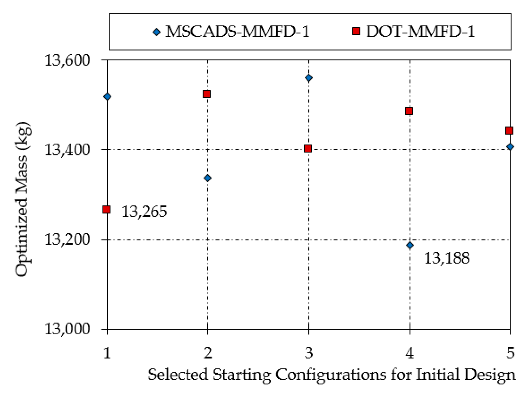
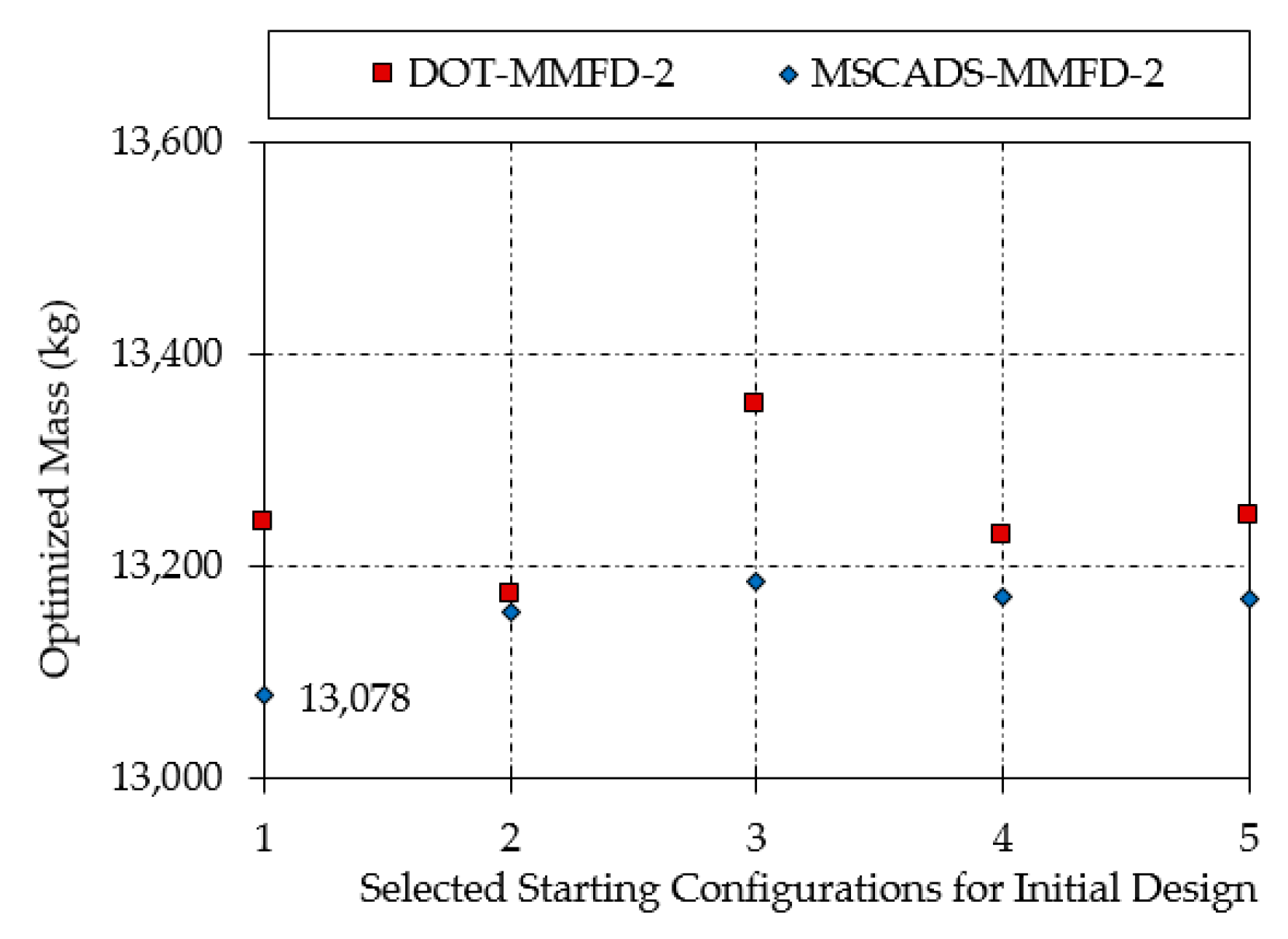
| Solution Type | Optimized Mass (kg) | ||||
|---|---|---|---|---|---|
| Min | 25% Max | 50% Max | 75% Max | Max | |
| MSCADS-MMFD-1 | 13,518 | 13,337 | 13,560 | 13,188 | 13,407 |
| DOT-MMFD-1 | 13,265 | 13,523 | 13,401 | 13,486 | 13,441 |
| MSCADS-MMFD-2 | 13,078 | 13,156 | 13,186 | 13,171 | 13,170 |
| DOT-MMFD-2 | 13,240 | 13,174 | 13,353 | 13,228 | 13,247 |
| Material Properties | T300/N5208 |
|---|---|
| Longitudinal modulus E11 | 181 GPa |
| Transverse modulus E22 | 10.3 GPa |
| In-plane shear modulus G12 | 7.17 GPa |
| Longitudinal tensile strength F1t | 1500 MPa |
| Longitudinal compressive strength F1c | 1500 MPa |
| Transverse tensile strength F2t | 40 MPa |
| Transverse compressive strength F2c | 246 MPa |
| In-plane shear strength F6 | 68 MPa |
| Density | 1600 kg/m3 |
| Major Poisson’s ratio ν12 | 0.28 |
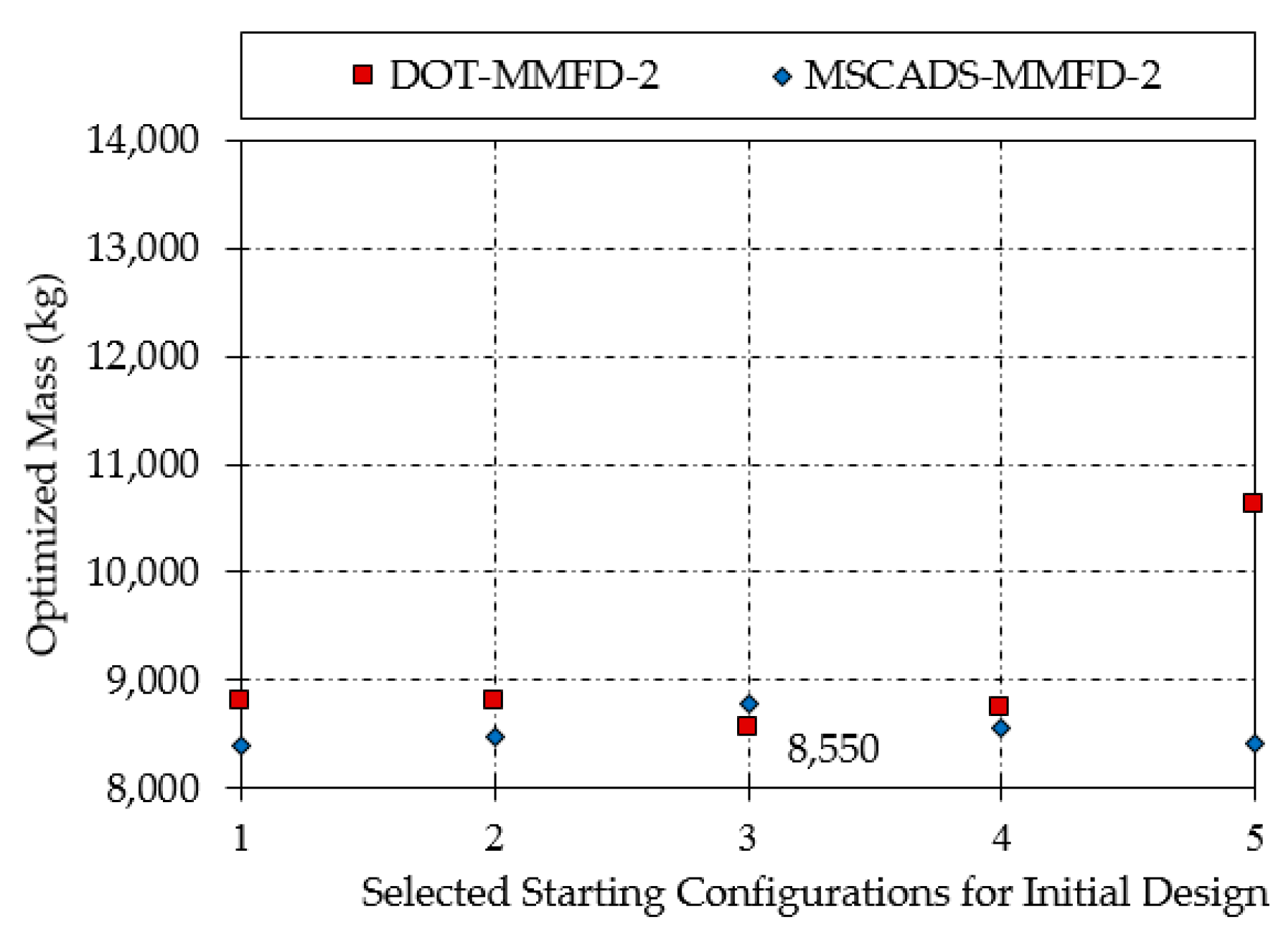
| Solution Type | Optimized Mass (kg) | ||||
|---|---|---|---|---|---|
| Min | 25% Max | 50% Max | 75% Max | Max | |
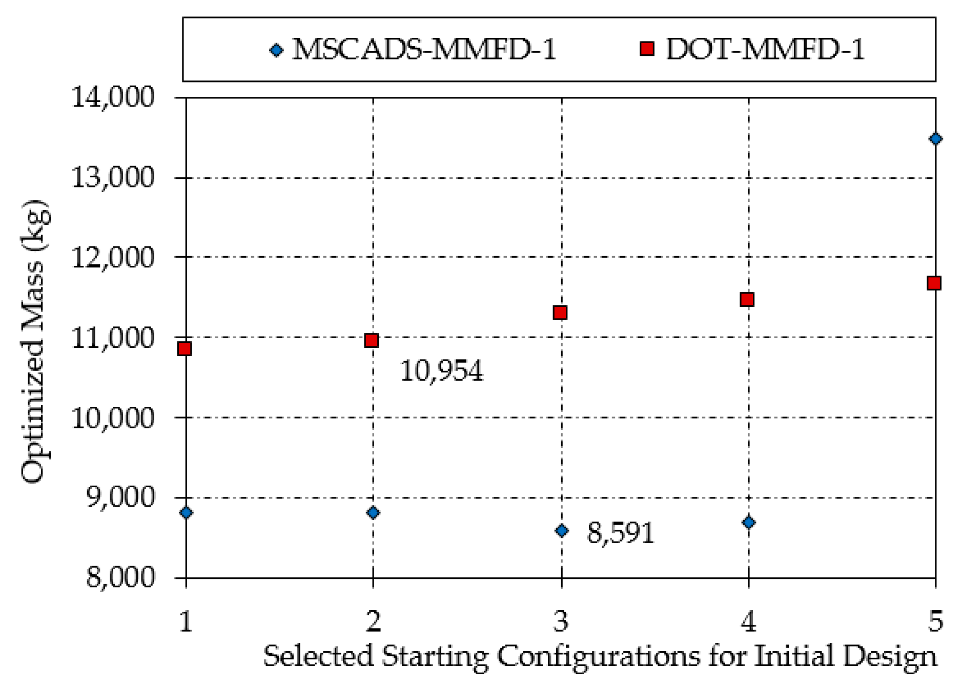
| MSCADS-MMFD-1 | 8816 | 8824 | 8591 | 8704 | 13,486 |
| DOT-MMFD-1 | 10,837 | 10,954 | 11,289 | 11,465 | 11,665 |
| MSCADS-MMFD-2 | 8389 | 8480 | 8788 | 8564 | 8415 |
| DOT-MMFD-2 | 8798 | 8806 | 8550 | 8750 | 10,630 |
© 2018 by the authors. Licensee MDPI, Basel, Switzerland. This article is an open access article distributed under the terms and conditions of the Creative Commons Attribution (CC BY) license (http://creativecommons.org/licenses/by/4.0/).
Share and Cite
Dababneh, O.; Kipouros, T.; Whidborne, J.F. Application of an Efficient Gradient-Based Optimization Strategy for Aircraft Wing Structures. Aerospace 2018, 5, 3. https://doi.org/10.3390/aerospace5010003
Dababneh O, Kipouros T, Whidborne JF. Application of an Efficient Gradient-Based Optimization Strategy for Aircraft Wing Structures. Aerospace. 2018; 5(1):3. https://doi.org/10.3390/aerospace5010003
Chicago/Turabian StyleDababneh, Odeh, Timoleon Kipouros, and James F. Whidborne. 2018. "Application of an Efficient Gradient-Based Optimization Strategy for Aircraft Wing Structures" Aerospace 5, no. 1: 3. https://doi.org/10.3390/aerospace5010003
APA StyleDababneh, O., Kipouros, T., & Whidborne, J. F. (2018). Application of an Efficient Gradient-Based Optimization Strategy for Aircraft Wing Structures. Aerospace, 5(1), 3. https://doi.org/10.3390/aerospace5010003