Abstract
The application of partitioned schemes to fluid–structure interaction (FSI) allows the use of already developed solvers specifically designed for the efficient solution of the corresponding subproblems. In this work, we propose and describe a loosely coupled partitioned scheme based on the recently introduced generalized-structure additively partitioned Runge-Kutta (GARK) framework. The resulting scheme combines implicit-explicit (IMEX) and multirate approaches while coupling of the subproblems is realized both on the level of the discrete time steps and at the level of interior Runge-Kutta stages. Specifically, we allow for varying micro step sizes for the fluid subproblem and therefore extend the multirate GARK framework based on constant micro steps. Furthermore, we derive the order conditions for this extension allowing for coupled time integration schemes of up to third order and discuss specific choices of the Runge-Kutta coefficients complying with the geometric conservation law. Finally, numerical experiments are carried out for uniform flow on a moving grid as well as the classical FSI test case of a moving piston.
1. Introduction
Coupled systems as in the context of fluid–structure interaction (FSI) often consist of subsystems with significantly different time scales. These subsystems may also deviate considerably in terms of their stiffness. In this context, using the same explicit time integration scheme with synchronous time steps for all subsystems might enforce very small step sizes which correspond to the small time scale components or those responsible for stiffness. On the other hand, a purely implicit method yields a large (possibly non-linear) coupled system of equations to be solved per time step. Therefore, it is reasonable to allow each subsystem of the coupled problem to advance with its preassigned time integration scheme which is adapted to its stiffness and time scales. In addition, it is sensible to evaluate slow components less often than fast ones.
In the context of fluid–structure interaction, several forms of mixed time integration approaches have been suggested. For example in [1], an implicit-explicit (IMEX) approach based on partitioned Runge-Kutta schemes allows for explicit coupling of the two physical fields, whereas the same implicit scheme for fluid and structure equations is used. A similar IMEX procedure is used in [2]. In [3,4], a multirate scheme referred to as subcycling is used to advance the fluid with small explicit time steps while an implicit scheme is used to discretize the structure equations using large time steps. Hereby, different forms of the subcycling procedure with respect to the treatment of the pressure forces at the fluid-structure interface and the sequencing of fluid and structure solves are investigated in terms of energy conservation. These algorithms fall into the category of loosely coupled partitioned methods. Generally, numerical approaches to the simulation of FSI phenomena can be classified into monolithic and partitioned solvers. Thereby, monolithic solvers are based on the direct discretization of the fully coupled problem which may then be linearized, e.g., by Newton’s method as in [5]. In partitioned approaches, suitable subsolvers, often already available, are used for each subsystem and suitable coupling conditions are devised, e.g., in [6,7]. While in the latter works, strong coupling is enforced using Newton’s method or fixed point iteration, respectively, a high order combined interface boundary treatment is devised in [8] in order to enhance the stability of loosely coupled schemes.
Similar to [1,2], we investigate the application of partitioned Runge-Kutta methods to fluid-structure interaction. Hence, this work fits into the category of loosely coupled partitioned schemes as no iterative methods are used for the coupling procedure itself. Nonetheless, as for the IMEX-Runge-Kutta approach in [1,2], the subsolvers are coupled at the level of interior Runge-Kutta stages in addition to the time levels corresponding to the chosen time step sizes. Furthermore, we combine the IMEX approach with the concept of multirate schemes which allows for different time step sizes of the subsolvers, corresponding to the subcycling strategy in [3,4].
The classical multirate idea for systems of ordinary differential equations dates back to the late fifties and was first studied by Rice [9]. Early multirate approaches were based on Runge-Kutta schemes [10,11], backward differentiation formulas [12,13,14], extrapolation schemes [15] or Rosenbrock-Wanner methods [16,17]. A drawback of these aforementioned early schemes is the fact that the coupling between slow and fast components of the system is done by interpolating and extrapolating state variables. This complicates the implementation into existing simulation packages [18]. Kværnø and Rentrop overcame this shortcoming by developing a concise theory of explicit multirate Runge-Kutta schemes and obtained promising results for electrical network simulations [19]. Deriving information by interpolation and extrapolation was circumvented by using the internal Runge-Kutta stages for coupling the integration schemes for the subsystems. In [18], a generalization to stiff problems was proposed. In that work, explicit Runge-Kutta schemes integrating the (nonstiff) fast system component are combined with linearly implicit Rosenbrock-Wanner schemes integrating the (stiff) slow system component.
IMEX partitioning is often used to term-split the corresponding partial differential equation, e.g., in the context of advection-diffusion-reaction equations, advection terms are classically discretized explicitly while viscous terms or stiff reaction is discretized by an implicit scheme [20,21,22]. IMEX-RK schemes have also been used in domain-based splittings, e.g., in [23] or based on eigenvalue estimates of the space discrete operators as in [24].
Very recently, Sandu and Günther [25] constructed a generalized-structure approach to additively partitioned Runge-Kutta (GARK) methods. This approach comes with a high level of flexibility and allows for different Runge-Kutta stage values as arguments of different components of the problem’s additively partitioned right-hand side. In addition, it combines different Runge-Kutta schemes with inter-component coupling based on the Runge-Kutta stages. In particular, it is possible to combine both the IMEX and the multirate approach. The GARK framework gives the intuition necessary to define new classes of additive schemes and eases the construction of additive schemes which preserve the order of the base ones. Günther and Sandu made use of the GARK framework to derive a multirate scheme solely based on implicit and explicit Runge-Kutta schemes [26]. Günther and Sandu’s multirate GARK scheme carries out just one so-called macro step of a “large” step size H within the slow component per iteration while at the same time carrying out several so-called micro steps of a “small” step size within the fast component per iteration, until both components “meet up” again. Hence, several equidistant micro time steps are carried out for one macro time step. The GARK formalism includes a variety of well-known schemes for partitioned problems, like the classical implicit-explicit (IMEX) Runge-Kutta schemes [20,23], as well as former multirate methods as in [19,21]. Furthermore, Günther, Hachtel and Sandu showed the feasibility of the multirate GARK approach for both implicit-implicit and implicit-explicit pairing of basic schemes [27] in the context of thermal-electrical coupling.
Concerning fluid–structure interaction, the time scales of the fluid subsystem are typically much shorter than the ones of the structure subsystem which makes the multirate GARK framework an attractive candidate. In contrast to the original application from electrical circuit simulation [18,19] and the test examples from thermal-electrical coupling [27], the fluid is expected to be stiff in many applications, which is the reason why implicit schemes often need to be applied to the fast fluid part. In case of (partially) explicit time integration of the fluid equations, e.g., in advection-dominated flow, the time steps may be requested to change gradually as a consequence of changes of the characteristic speeds. In case of implicit time integration, the fast fluid step sizes (the micro steps) may have to vary during the structure step (the macro step) due to the convergence behavior of the nonlinear solver or due to error control.
Therefore, in this work, we seek to overcome the major restriction of keeping the micro step sizes constant, by allowing varying micro step sizes that may be adapted according to error or stability requirements. The multirate GARK framework is thus extended towards the adaptive choice of micro time steps within one macro time step. In this work, the corresponding order conditions are derived. Furthermore, we investigate the choice of coupling coefficients which allows the combined method to preserve the order of the single schemes within the partitioned approach. We then derive specific multirate GARK schemes applicable to mechanical fluid–structure interaction, give details regarding compliance with the geometric conservation law and show numerical results for the classical fluid–structure interaction problem of a moving piston.
This paper is structured as follows. Section 2 reviews the concept of partitioned Runge-Kutta schemes for partitioned ordinary differential equations including the recently introduced GARK approach. In Section 3, the concept of adaptive micro step sizes is introduced in order to obtain flexible multirate GARK (MGARK) schemes for coupled problems. We then derive the corresponding order conditions for this extension of the multirate GARK scheme given in [26]. Thereafter, we formulate the adaptive micro step MGARK scheme for mechanical fluid-structure interaction and discuss the resulting restrictions to the specific structure of the base methods as well as to the coupling coefficients. Our approach to time adaptivity based on embedded error estimation is then presented in Section 3.4. Numerical experiments are presented in Section 4. Here, compliance with the geometric conservation law is demonstrated for uniform flow on an artificially moving grid, the viability of adaptive micro steps is shown by an investigation of the step size statistics and finally, we investigate the efficiency of higher order time integration for small tolerances by a comparison of first, second and third order schemes in terms of error vs. CPU time.
2. Partitioning Systems of Ordinary Differential Equations
We may generally distinguish two kinds of partitioned systems of ordinary differential equations. The complete system under consideration may be composed of different subsystems, each subsystem containing a specific subset of the given equations. The system is then partitioned by component. Else, if the right hand side of the ODE contains different terms of very different character as in the context of conservation laws containing convective and diffusive fluxes, usually the right hand side of the ODE is additively partitioned as in the following definition.
Definition 1.
Let and for . A system of (autonomous) ordinary differential equations of the form
for is called an additively partitioned system of ordinary differential equations. Adding initial conditions
we obtain an additively partitioned initial value problem.
Every component-partitioned system may obviously be rewritten as an additively partitioned system of the same dimension inserting zeros into suitable positions of the right hand side terms. Therefore, we will restrict the discussion to the more general case of additively partitioned systems at this point.
For the numerical solution of additively partitioned initial value problems, Kennedy and Carpenter [22] constructed specific Runge-Kutta schemes called additive Runge-Kutta schemes (ARK). The ARK schemes apply different Runge-Kutta methods , , to the terms on the right hand side of the ODE in the following form:
with the corresponding Butcher table
in which the individual Runge-Kutta schemes have the same number of stages s. For the special case of , an equivalent class for the solution of component-partitioned systems is given by Hairer et al. ([28], [II.15]). Sandu and Günther [25,26] extended the ARK schemes to the so-called generalized-structure additively partitioned Runge-Kutta (GARK) schemes. The most general form of a GARK scheme is given by the following definition.
Definition 2.
A GARK scheme for the numerical solution of a D-times partitioned initial value problem (see Definition 1) with GARK stages and step size h is given by
where is a map which determines which of the stage values is assigned to the k-th right hand side term. We denote this scheme by GARK.
The corresponding generalized Butcher table reads
In [25], Sandu and Günther have shown that GARK schemes are equivalent to ARK schemes in the sense that, on the one hand, every ARK scheme can be written as GARK scheme with J given by the map , and on the other hand, every GARK scheme can be written as an (artificially enlarged) ARK scheme.
As an example illustrating the generality of the GARK formulation, we may consider the classical fractional-step-θ scheme introduced in [29] which is widely used for time integration of the Navier-Stokes equations. Given an additively split ordinary differential equation
the fractional-step-θ method reads
Setting , we may rewrite this scheme as a four-stage ARK scheme as defined in Equations (3) and (4) using the Butcher table
There are several ways to write the fractional-step-θ method as a GARK scheme. A trivial way of achieving that is to set and , which results in a GARK scheme with the generalized Butcher table
Another possible representation of the fractional-step-θ method within the GARK framework that makes use of different GARK stages is given by setting , , , . With these GARK stage values the scheme can be written as a GARK scheme with the corresponding generalized Butcher table
This formulation gets rid of the zero columns of the above ARK/trivial GARK formulation of the scheme.
GARK schemes which assign to each term of the right hand side of Equation (1) a specific stage value are particularly convenient, as the general definition further simplifies.
Definition 3.
GARK schemes with separate stage value for each right hand side term of a D-times partitioned initial value problem (see Definition 1) result from the choice and within the general GARK scheme. They are given by
We denote this scheme by GARK = GARK.
3. Multirate GARK (MGARK) Schemes
For splittings into two time scales, i.e., for , which is a reasonable starting point for problems in the context of fluid–structure interactions, we now define the multirate generalized-structure additively partitioned Runge-Kutta (MGARK) schemes as follows.
Definition 4 (MGARK scheme).
An MGARK scheme using micro steps of step size () for fast components and a macro step of step size H for slow components is given by
Thus, one step of an MGARK scheme includes one macro step of step size H as well as all of the N micro steps having potentially different step sizes . In order to apply the order theory for GARK schemes as in Theorem 1 to MGARK schemes, we would like to reformulate the MGARK method as a GARK scheme using separate stage values for fast and slow components as in Definition 3. As the classical form of GARK schemes depends on constant micro step sizes within one macro step, the step size of the micro steps will be denoted by using the coefficients . Substituting these step sizes into Equations (9)–(11) and considering the coefficients as modifications to the Runge-Kutta coefficients , and , we obtain
From Equations (12)–(14) it is in fact obvious that the MGARK scheme is equivalent to a GARK scheme with the corresponding generalized Butcher table
containing the coefficients .
3.1. Order Conditions for MGARK Schemes with Variable Micro Steps
The order conditions of GARK schemes have been explicitly derived by Sandu and Günther up to schemes of 4th order, see [25]. The derivation is based on the application of the theory of N-trees by Araújo et al. [30] on the representation of the GARK scheme in Equations (5) and (6). In order to obtain simple formulations for these order conditions, we denote by “·” the usual scalar product of two vectors as well as the usual matrix vector product while the symbol “*” denotes a component-wise multiplication of two vectors.
Theorem 1
(GARK order conditions; Sandu and Günther ([25], Theorem 2.6)). For , we define . We have the following order conditions for the GARK scheme as in Definition 2, where :
First order
Second order
Third order
Fourth order
Now, the application of the GARK order conditions to the Butcher table given in Equation (15) yields the following assertion.
Theorem 2 (MGARK order conditions).
We define , , , . The following conditions are sufficient to obtain the desired order of an MGARK scheme.
First order
Second order
Third order
and
Remark 1.
In [26], order conditions for multirate GARK schemes using constant micro step sizes within the macro step are presented. These order conditions require that all micro steps taken in the same macro step have the same step size. Of course, micro step sizes may change after the macro step is completed. The conditions given in Theorem 2 are thus more general because they allow for varying micro step sizes also within the macro step. In the special case of constant micro step sizes per macro step we recover the order conditions in [26].
Proof of Theorem 2.
We apply the order conditions of Theorem 1 to the Butcher table of the MGARK scheme given in Equation (15). Herein, the conditions have to be applied to the underlined quantities. The assertion is proven if each order condition of Theorem 1 holds due to an equivalent order condition or due to a subset of order conditions formulated in Theorem 2. First, we remark when requiring the conditions (24), (27), (31) and (33) we assume in particular that the corresponding fast base method is at least of the same order as the coupled scheme.
- Second order conditions: Equation (17) for can be rewritten asusing Equations (24) and (27). The corresponding condition on the right hand side is then fulfilled due to Equation (26). Equation (17) for and for is directly equivalent to Equations (29) and (30), respectively, while leads to Equation (28).
- Third order conditions (Part 1): Equation (18) for rewrites asUsing Equations (24), (27) and (31) this is equivalent toAs before, this condition is valid due to Equation (26). For and , Equation (18) yieldsDue to the equality for an arbitrary vector , this condition is equivalent to Equation (37). For , Equation (18) directly rewrites as Equation (38). The two choices and for Equation (18) lead to the Equation (39). The remaining choices of in Equation (18) finally yield the condition (40) for and the condition (32) for .
- Third order conditions (Part 2): Equation (19) for can be rewritten asUsing Equations (24), (27) and (33) this is equivalent toi.e., validity follows from Equation (26). For , Equation (19) rewrites asConsidering Equation (24), this is equivalent to Equation (41). Furthermore, for , , , , and , Equation (19) rewrites as Equations (42), (35), (36), (44), (43) and (34), respectively. ☐
The order conditions as in Theorem 2 include the assumptions that the fast base method is at least of the same order as the coupled scheme and that the sum of micro step sizes is equal to the size of the macro step. This assumption is incorporated into the Equations (24), (27), (31), (33), respectively, depending on the considered order, as well as the Equation (26). Thus, the MGARK order conditions of Theorem 2 are sufficient, but not necessary. In fact, this degree of freedom within the MGARK scheme can already be observed in the method formulation given in Equations (12)–(14) as well as on the left side of the right hand side Butcher table in Equation (15).
However, in this work, we will only consider MGARK schemes which fulfill the above assumptions. In this case, the conditions in Theorem 2 become necessary and the order of the complete MGARK scheme is restricted by the minimum order of the respective base methods. In order to achieve this maximum order, the coupling Equations (29) and (30), (35) and (36), (37)–(44) have to be fulfilled. This can be achieved by a suitable choice of the coupling coefficients and .
In addition, we would prefer internally consistent MGARK schemes as they already fulfill a significant number of the order conditions in Theorem 2 which leads to a considerable simplification. According to [25], internally consistent GARK schemes are defined as follows.
Definition 5.
A GARK scheme given by Definition 2 is internally consistent, if
holds for all .
According to the notation of MGARK schemes used in Definition 4 and specified by the generalized Butcher table in Equation (15), the above definition of internal consistency takes the form and in case of an MGARK scheme. For internally consistent MGARK schemes, the order conditions in Theorem 2 simplify to
Theorem 3 (Order conditions for internally consistent MGARK schemes).
An internally consistent MGARK scheme as specified by Definitions 4 and 5 is at least of first order if Equations (24)–(26) hold. The scheme is at least of second order, if in addition to the first order conditions the Equations (27) and (28) hold. The scheme is at least of third order, if in addition to the second order conditions the third order conditions for the individual schemes, i.e., Equations (31)–(34) as well as the coupling Equations (35) and (36) are fulfilled.
Proof.
Let , . For an internally consistent MGARK scheme, Definition 5 and the subsequent remark yield
These two above conditions are equivalent to
We will show that the sufficient conditions stated in Theorem 2 are fulfilled. For first order, nothing has to be shown as the above first order conditions are precisely the ones in Theorem 2.
- Third order conditions (Part 1): The validity of Equations (37)–(40) needs to be shown. Both of the Equations (37) and (38), in combination with Equation (45), reduce toDue to Equations (24), (27) and (31), the above equations further reduce towhich is fulfilled due to Equation (26). Furthermore, the validity of the Equations (39) and (40) immediately follows from Equations (32) and (46).
- Third order conditions (Part 2): Finally, the validity of Equations (41)–(44) remains to be shown. Using Equations (24), (27), (33) and (45), Equation (41) reduces toand is thus fulfilled due to Equation (26). The validity of the Equation (43) follows from Equations (34) and (46). Considering Equations (45) and (46), Equations (42) and (44) are equivalent to Equations (35) and (36), respectively. ☐
The only coupling Equation (26) of the general MGARK scheme is thus required also for internally consistent MGARK schemes. However, the two second order coupling conditions are automatically fulfilled for internally consistent MGARK schemes without requiring additional conditions. The large number of third order coupling conditions of the general MGARK scheme given in Theorem 2 now reduces to only the two coupling Equations (35) and (36).
Concerning the concrete choice of an MGARK scheme in practice, we notice that the computational effort needs to be low enough in order to not exceed the cost of solving the coupled system with constant micro step sizes per macro step. Coupling the calculation of the slow components to all micro steps seems impractical from this point of view. The reasonable partial decoupling of the macro step calculation from the micro step computations has already been suggested by Günther et al. [18,26]. Their approach consists in coupling the macro step only to the first micro step. Formally this is realized by setting for .
3.2. Specific Coupling Conditions Retaining the Order of the Base Schemes
In the following, we consider specific choices of base methods and and the corresponding choice of coupling conditions which retain the order of the base methods. Herein, we always assume that the Equation (26) holds, i.e., we have . We consider the following cases which are ordered from general to specific ones.
- (a)
- The base methods both have s stages and the macro step may be coupled to all of the N micro steps.
- (b)
- The base methods both have s stages and the macro step is only coupled to the first of the N micro steps.
- (c)
- The base methods may be either explicit first stage, singly diagonal implicit Runge-Kutta (ESDIRK) or explicit methods having 4 stages and the macro step is only coupled to the first of the N micro steps. With , we additionally assume , , , .
From Theorem 2 we immediately obtain
Corollary 1 (First order coupling).
For all of the cases (a)–(c), the MGARK scheme is at least of first order if this is true for the base methods—irrespective of the concrete choice of coupling.
Corollary 2 (Second order coupling).
If the coupling is realized as
Choice A
and
or
or
Choice B
and
then the MGARK scheme is at least of second order, if this is true for the base methods.
Proof.
With the Equation (47), the Equation (45) is fulfilled and with Equation (48) or (49), respectively, also Equation (46) holds, which is equivalent to the internal consistency of the MGARK scheme. Equations (50)–(52) obviously lead to an internally consistent MGARK scheme as well. According to Theorem 3, internally consistent MGARK schemes do not have to fulfill additional coupling conditions in order to achieve second order. ☐
Corollary 3 (Third order coupling).
If in case (c) the coupling is realized as
and
the MGARK scheme is at least of third order, if this is true for the base methods.
Proof.
The advantage of the presented coupling strategies is given by the fact that neither the micro step size (and thus ) nor the final number N of micro steps per macro step needs to be known a priori. Only the macro step size H is provided while the micro step sizes may be varied adaptively in the process of taking micro steps. For each micro step, the coupling coefficients will be newly adapted to the micro step size. Switching on the coefficient in the last micro step ensures the coupling condition Equation (35). The number of micro steps is thereby irrelevant, the scheme only has to identify the last micro step. Since the slow component is only coupled to the fast component within the first micro step, the corresponding coupling condition Equation (36) is already fulfilled by the specific choice of the parameter in the first micro step.
3.3. Application of MGARK to Coupled Problems of Fluid–Structure Interaction
For mechanical fluid–structure interaction, the fluid domain is time-dependent. In order to deal with such moving fluid domains, the arbitrary Lagrangian-Eulerian(ALE) formulation for the fluid variables on a time-dependent domain is used in this work. The ALE formulation is given by
see [1,31]. The fluid equations will then be discretized by a finite volume method based on the cell means of the conservative variables and cell volume, i.e.,
Rewriting the discretized right hand side as a function , which incorporates a numerical flux function, we obtain a system of ordinary differential equations of the form
Herein, the fast components are given by the fluid variables, i.e., and the slow components will be obtained from the deformation of a structure which influences the fluid domain and thus determines the cell sizes, i.e., . Thus, Equation (56) may be written as
where denotes grid velocities which will be determined by the so-called geometric conservation law (GCL). The GCL basically states that constant solutions have to be preserved by the discretization, i.e., constant states are exact solutions of Equation (56). This can be formulated by the condition
where denotes the discretization of
corresponding to , see [31]. The application of a Runge-Kutta scheme with step size h to the system on the right hand side of Equation (58) yields
In case of an explicit method with for , Equation (59) provides a successive determination of grid velocities , …, . In addition, if , the final grid velocities can be calculated from Equation (60). Thus, the grid velocities are solely determined by the cell volumes at internal stage time levels and hence by the corresponding structure states. We have to keep in mind that the determination of for needs the cell volumes at the successive Runge-Kutta stage following the current stage i while the velocities are determined from the cell volumes at the end of the Runge-Kutta step. The precise calculation of these values in the context of an MGARK scheme is given in Algorithm 1 and the corresponding description. As in [31] we may require Equations (59) and (60) to hold face-wise, i.e.,
where is the face integrated grid velocity and and , denote the volume change due to the moving face E at the i-th Runge-Kutta stage and at time , respectively.
In particular, in the situation of one spatial dimension, we obtain a relation to the grid point positions ,
In the context of fluid–structure interaction, we rewrite the MGARK method in the more convenient component partitioned form. In addition, we explicitly use the intermediate values of the fast components at the intermediate micro step times and introduce the stage derivatives and in order to avoid unnecessary function evaluations.
The MGARK scheme with micro steps of step sizes () for the fast components and a macro step of step size H for the slow component is then given by
with stage derivatives
based on the stage vectors
In case of fluid–structure interaction problems, where the evaluation of the fluid right hand side depends on the grid velocities, Equation (70) needs to be replaced by
where the grid velocities need to be computed in accordance with the GCL.
We note that the MGARK scheme in the above form given in Equations (65)–(75) may be still be fully coupled, i.e., in order to compute the stage derivatives and the iterative solution of the above coupled equations may be necessary.
Hence, in the following, we consider an efficient implementation of the MGARK scheme given in Equations (65)–(75) for the numerical solution of coupled fluid-structure interaction. As base methods, we choose an explicit method for the fast components, i.e., the fluid variables, as well as a diagonally implicit Runge-Kutta (DIRK) scheme for the slow components, i.e., the structure variables. For efficiency reasons, we couple the macro step only to the first micro step. In this way, the stage derivatives of the slow component are calculated together with the corresponding stage derivatives of the fast components in the first micro step. In the subsequent micro steps (), only the remaining stage derivatives of the fast components need to be calculated.
| Algorithm 1 MGARK algorithm for coupled problems with moving grids respecting the GCL. | ||
| 1: | procedure MGARK() | |
| 2: | ||
| 3: | for λ← 1 to N do | loop over micro steps |
| 4: | for i← 1 to do | loop over Runge-Kutta stages |
| 5: | if then | |
| 6: | if then | calculation of MGARK stage derivatives of the structure |
| 7: | ||
| 8: | ||
| 9: | ||
| 10: | end if | |
| 11: | if then | |
| 12: | macro update of the structure | |
| 13: | end if | |
| 14: | end if | |
| 15: | if then | calculation of MGARK stage derivatives of the fluid |
| 16: | ||
| 17: | ||
| 18: | MeshVelocity | GCL-compliant grid velocities |
| 19: | ||
| 20: | end if | |
| 21: | if then | |
| 22: | micro update of the fluid | |
| 23: | end if | |
| 24: | end for | |
| 25: | end for | |
| 26: | macro update of the fluid | |
| 27: | return | |
| 28: | end procedure | |
| Algorithm 2 Computation of GCL-compliant mesh velocity | ||
| 1: | procedure MeshVelocity | |
| 2: | if then | not the last stage within current micro step |
| 3: | ||
| 4: | Solve for | |
| 5: | else | |
| 6: | if then | last stage within current micro step, not the last micro step within current macro step |
| 7: | ||
| 8: | else | last stage within current micro step, last micro step within current macro step |
| 9: | ||
| 10: | end if | |
| 11: | Solve for | |
| 12: | end if | |
| 13: | return | |
| 14: | end procedure | |
Algorithms 1 and 2 summarize the concrete procedure for the implementation of the MGARK scheme for fluid–structure interaction including GCL-compliant grid velocities. The preservation of the GCL is guaranteed by computing the grid velocities in accordance with Equations (59) and (60). In Algorithm 1, line 18, the velocities are determined by the procedure MeshVelocity defined in Algorithm 2.
The efficiency and practicability of the scheme formulated in the above Algorithms 1 and 2 requires additional conditions concerning the chosen base methods and the coupling coefficients.
- The decision to couple the structure macro step solely to the first fluid micro step for efficiency reasons reduces the second condition Equation (46) of internal consistency toIn order to access only the already determined fluid stage derivatives of the first micro step when calling Algorithm 1, line 7 the condition for is necessary, in particular, we need to set for . This does only agree with Equation (76) if holds, i.e., if the first stage of the slow base method is an explicit stage. This requires using an E(S)DIRK scheme instead of an (S)DIRK scheme if internal consistency is to be guaranteed. However, without internal consistency, determining suitable coupling coefficients would require significantly more effort, as can be seen in Theorems 2 and 3.
- In order to access only the already determined structure stage derivatives when calling Algorithm 1, line 17, the condition for is necessary. For the coefficients with no additional conditions have to be fulfilled as at the end of the first micro step, all structure stage derivatives have been calculated and can be accessed.
- The construction of suitable structure states for the determination of GCL-compliant mesh velocities according to Algorithm 2 poses additional restrictions to the choice of the coupling parameters. From line 3, we obtain the stronger condition for . From line 7, we also obtain a condition for the coupling parameters of the second micro step which takes the form for . However, this condition is only relevant in the case .
- The first condition Equation (45) of internal consistency for is given bywhich in combination with the above points leads to the additional condition .
- In Algorithm 2, line 9 the value of is accessed if , . If , this value has already been determined in Algorithm 1, line 12. However, if this value is only available if .
- For an explicit base method , the computation of mesh velocities in Algorithm 2, lines 4 and 11 requires nonzero entries of and .
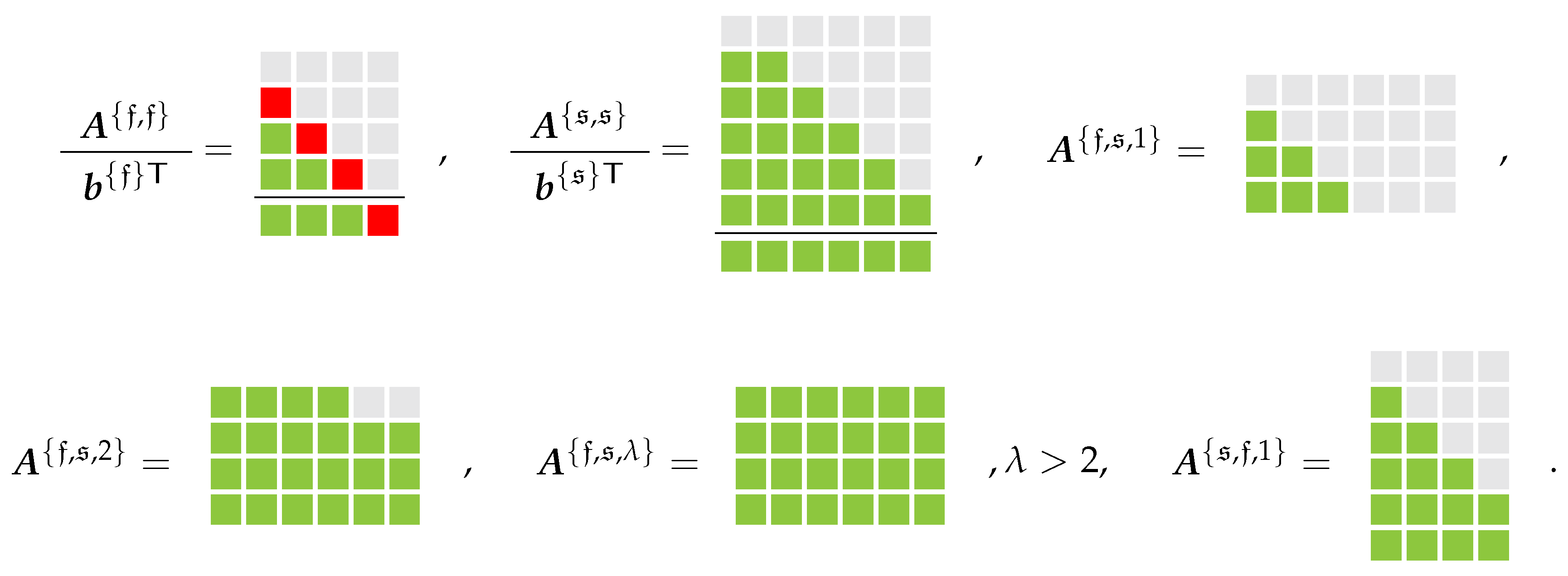
In summary, we may specify the structure of the base methods in the following form, visualized in Figure 1 for , . Here, the gray-colored blocks (  ) denote zero entries while the red ones (
  ) denote entries required to be non-zero in agreement with our strategy of enforcing the GCL and the green-colored blocks (
  ) symbolize arbitrary entries.
) denote zero entries while the red ones ( ) denote entries required to be non-zero in agreement with our strategy of enforcing the GCL and the green-colored blocks ( ) symbolize arbitrary entries.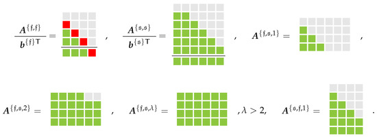
Figure 1.
Required structure of base methods. Gray-colored blocks denote zero entries, red-colored blocks denote entries required to be non-zero, green-colored blocks symbolize arbitrary entries.
Looking at the required structures of and in Figure 1, suitable coupling parameters to achieve overall second order are given by the choice of according to Equations (50) and (51) and of according to Equation (52), while the choice given by Equations (47) and (49) does not conform to items 1, 3 and 4 given in the above discussion. Concerning third order MGARK schemes, the coupling conditions given by Equations (53)–(55) agree to all of the above requirements.
We further remark that the determination of in Algorithm 1, line 9 may be implicit. Prescribing an (E)SDIRK scheme as slow base method, a potentially nonlinear system of equations has to be solved for , given by
combining lines 8 and 9 in Algorithm 1.
3.4. Time Adaptivity
Efficiency for practical applications needs time adaptivity. Hence, the macro and micro step sizes will be adaptively chosen depending on an error estimator based on embedded Runge-Kutta methods. The discrete macro time levels are then given by
and the discrete micro time levels are
where is the number of micro steps within the n-th macro step and the micro time levels relate to the macro time levels as and .
Figure 2 illustrates the potential positions of discrete macro and micro time levels. The concrete computation of macro and micro step sizes depends on error control using the parameters , and as well as the relative and absolute tolerances and according to Algorithms 3 and 4.
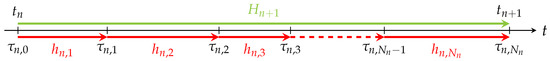
Figure 2.
Depiction of macro and micro step sizes including corresponding notation.
Since the final number of micro steps within the n-th macro step is not known a priori, Algorithm 4 is devised to work without this information. For the present adaptivity strategies, the first macro step size as well as the first micro step size need to be prescribed. All other step sizes are then automatically calculated by the given Algorithms. This time step calculation can then be combined with CFL based time step computation depending on the specific set-up of a numerical test case. The corresponding details will be clarified in Section 4.
| Algorithm 3 Adaptive step size determination for macro step with step size . |
|
| Algorithm 4 Adaptive step size determination for micro step with step size . | ||
| 1: | procedure adapt_micro_step_size() | |
| 2: | ||
| 3: | ||
| 4: | if then | |
| 5: | ||
| 6: | ||
| 7: | if then | not the last micro step within current macro step |
| 8: | ||
| 9: | Accept solution and employ step size in the next micro step | |
| 10: | else | last micro step within current macro step |
| 11: | ||
| 12: | Accept solution and employ step size in the first micro step | |
| of the next macro step | ||
| 13: | end if | |
| 14: | else | |
| 15: | ||
| 16: | Repeat micro step with new step size | |
| 17: | end if | |
| 18: | end procedure | |
4. Numerical Experiments
In the following numerical experiments, the considered MGARK schemes are constructed from base methods of second and third order, respectively. These base methods are given in the form
where denotes the embedded method to the base method such that if p is the order of the base method and denotes the order of the embedded method, we have .
Second order base methods
A second order MGARK scheme is derived from the explicit Heun method (, ) and the implicit trapezoidal rule (, ) which is an ESDIRK scheme.
| Explicit Heun scheme | Implicit trapezoidal rule |
Third order base methods
A pair of third order base methods from which we construct the third order MGARK scheme is given by the following four-stage RK schemes of order and embedded order which is taken from [32]. The corresponding IMEX scheme is denoted by IMEXRKCB3c in that work.
RK explicit 3rd order
3rd order DIRK scheme
4.1. Constant Flow with Prescribed Grid Movement
First, to check the viability of our implementation concerning the preservation of the GCL, we apply the MGARK approach to constant flow with an artificial grid movement.
Hence, we consider constant solutions of the initial value problem
If the initial conditions is given by a constant initial state , , the exact solution is constant in time and space, for , hence we expect the numerical approximation of to be constant as well. Starting from an initial grid , , the method runs on a time-dependent spatial discretization
where the grid points are moved according to the rule
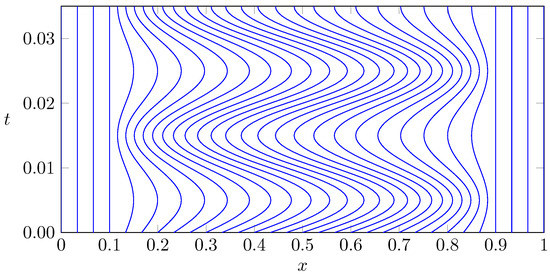
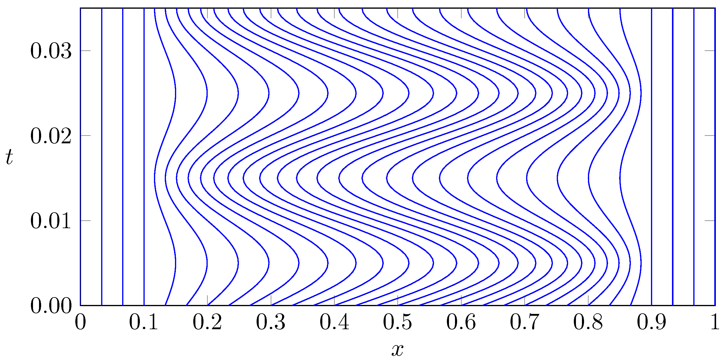
with the parameters and . The grid cells are then determined from the grid points according to . Hence, in this set-up the grid points with are fixed while the grid points with oscillate in form of a sine wave in time with frequency ω. The choice of the amplitude according to Equation (81) guarantees that the grid cells do not overlap, i.e., for all , we have . Figure 3 depicts the corresponding grid motion for an equidistant initial grid with cells, a frequency of and a confined region of grid movement bounded by , .
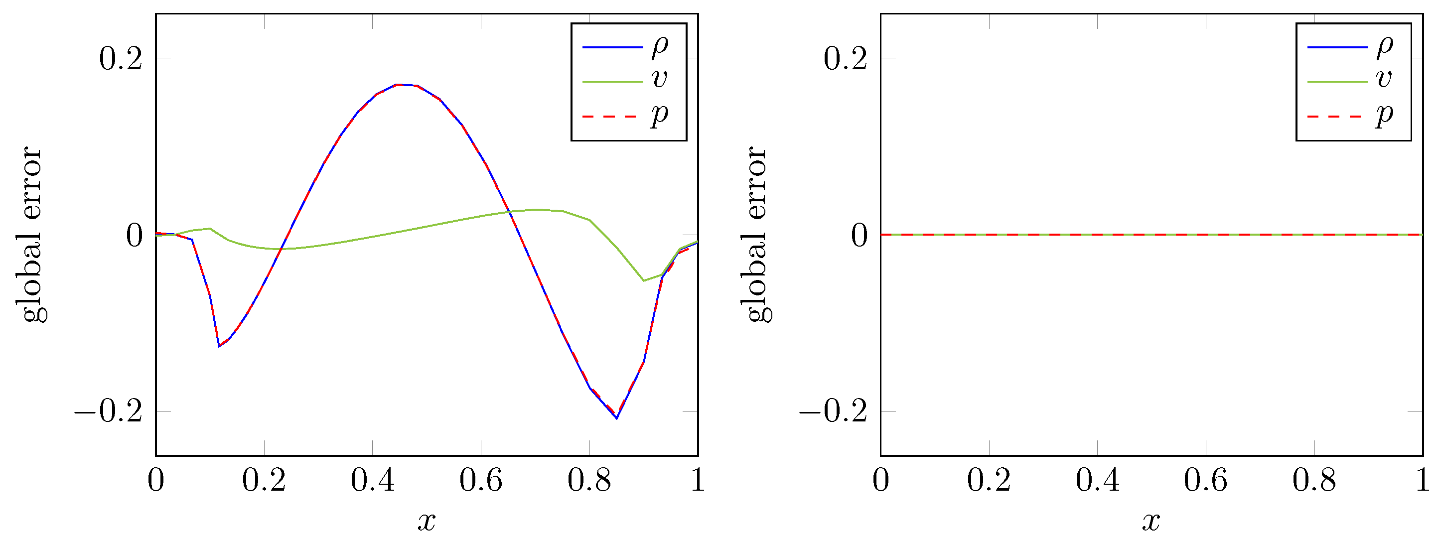
In order to illustrate the importance of calculating mesh velocities which are consistent with the GCL, Figure 4 depicts the error with respect to density, velocity and pressure of the explicit Euler scheme applied to the fluid equations. More precisely, the right hand side of Figure 4 shows the result for mesh velocities computed according to Equations (59) and (60) while the left hand side depicts the corresponding errors obtained by grid velocities determined from differentiation of Equations (80) and (81) with respect to t. In the first case the constant initial state is preserved in accordance with the theoretical considerations while the second case does not lead to a numerical method consistent with the GCL.
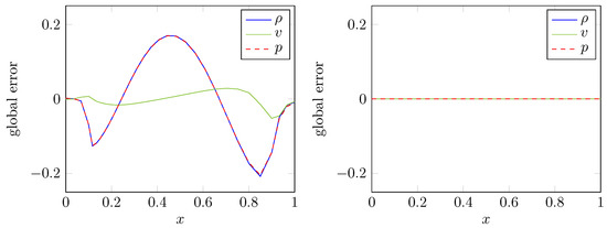
Figure 4.
Global error with respect to density, velocity and pressure at time for explicit Euler scheme with step size applied to constant flow. Left: Use of exact grid velocities; Right: Computation of grid velocities consistent with the geometric conservation law (GCL).
Now we simulate this test case using the proposed MGARK scheme. In order to obtain a partitioning in fast and slow components, we consider the autonomous coupled system composed of the fluid variables as the fast components and the grid points as well as the time variable as slow components. Therefore, the grid motion given in Equations (80) and (81) is not prescribed exactly but provides a differential equation for the slow components of the coupled system. The slow components are hence evolved according to
starting from a given initial state . Due to the ALE formulation Equation (56) of the fluid equations, the fast components are given by the products of the cell averages of the conservative fluid variables with the corresponding cell volumes. By the construction just described, the slow components are given by and the coupling between these subsystems now takes the form and , which shows that the evolution of slow components is actually independent of the fast ones in this case.
Figure 5 depicts the experimental order of convergence obtained by two different choices of base methods. The results on the left hand side are obtained by choosing the IMEXRKCB3c explicit/implicit schemes (78) and (79), i.e., the explicit third order scheme for the fast fluid component and the implicit third order scheme for the slow mesh movement component together with coupling conditions as given in Corollary 3. The right hand side shows the results obtained when replacing the explicit IMEXRKCB3c scheme with first order explicit Euler scheme for the fluid equations and setting all coupling coefficients to zero.
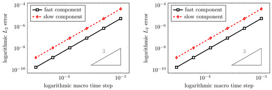
Figure 5.
Experimental order of convergence. Left: Base methods IMEXRKCB3c (explicit/implicit) of third order; Right: Explicit Euler scheme for fast components, third order implicit base method of IMEXRKCB3c for slow components.
First of all, we observe that the chosen coupling strategies lead to an experimentally obtained convergence of third order. Though at first sight, it is striking that a global convergence of third order is also obtained using a fluid time discretization of only first order, we recall that our GCL-consistent MGARK scheme does not produce any disturbances of the constant fluid state, independent of the order of the fast base method. Hence, the global error is only determined by the slow base method which approximately determines the grid positions. Thus, the slow method solely determines the order of the coupled scheme in this case. However, in general, the accuracy of the coupled scheme reduces to first order if one of the base methods is only of first order.
4.2. The One-Dimensional Piston Problem
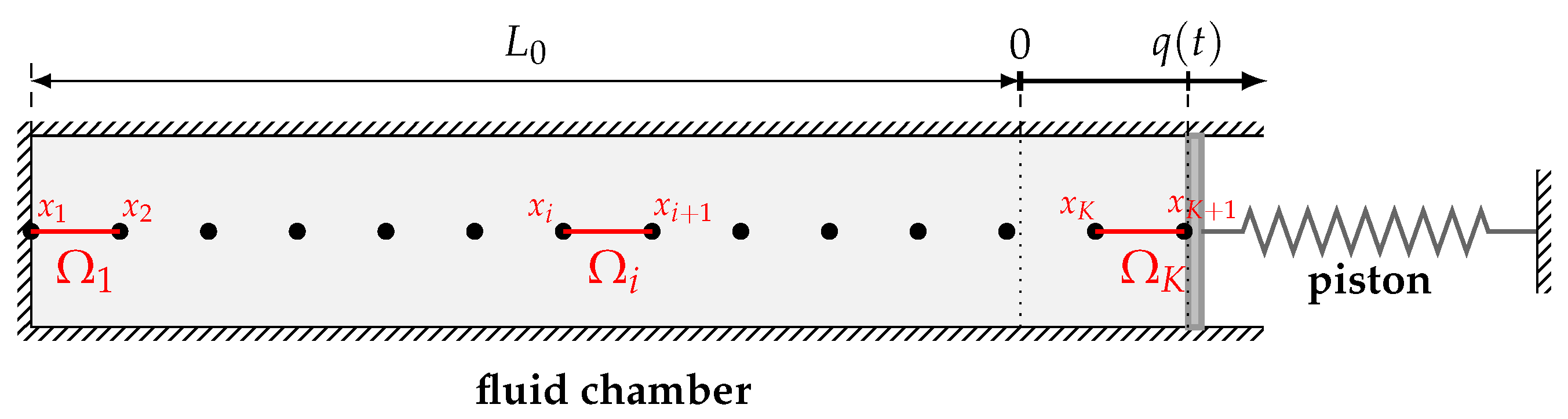
The interaction between a piston which is attached to a spring and an inviscid fluid which is contained in a chamber is a classical test case in the context of fluid–structure interaction [33,34]. The coupled piston problem and its one-dimensional set-up are illustrated in Figure 6.
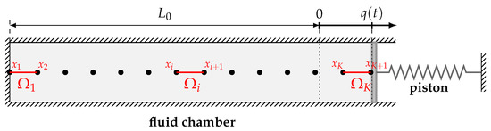
Figure 6.
One-dimensional piston problem.
In the mathematical formulation, the fluid is described by the one-dimensional inviscid Euler equations while the displacement of the piston is modelled by an undamped harmonic oscillator. In non-dimensional form we obtain a coupled system of the fluid equations given by
with
where and p denote density, velocity, specific total energy and pressure of the fluid, respectively, while γ denotes the adiabatic coefficient, and the structure model for the piston displacement given by
where the parameters in this non-dimensional formulation correspond to the mass m and the stiffness k of the spring as well as the cross-sectional area A of the piston as well as its initial displacement and velocity . The piston displacement determines the length of the time-dependent fluid domain according to
This domain is discretized by a constant number of grid cells, cf., Figure 6. Let denote the grid points such that . The influence of the fluid subsystem on the structure subsystem is given by the difference of the fluid pressure acting on the piston at the fluid-structure interface, i.e., the right boundary of the fluid domain and the ambient pressure .
The specific setting of the piston parameters and and the initial length of the fluid domain as well as the initially constant fluid variables , , and the initial piston displacement and velocity , which have been used in this test case are summarized in Table 1.

Table 1.
Parameters and initial conditions for piston problem.
We may now take a closer look at the difference in time scales for the fluid and structure subsystems in this set-up. The characteristic time scale of a fluid is given by the time needed by a pressure wave to traverse the chamber, i.e.,
where c denotes the sound speed. For the values given in Table 1 we obtain .
The characteristic time scale of the structure is determined by the oscillation period, i.e.,
whereby we obtain for the values in Table 1.
The one-dimensional Euler equations in ALE formulation are then discretized by a finite volume method which yields
for interior grid cells, using a suitable numerical flux function . At the two boundaries of given by the grid points and , boundary conditions are required. As there is no movement of fluid particles through the boundaries of the fluid chamber (no-slip conditions), we demand that at the boundaries, the fluid moves with the same velocity as the corresponding boundary grid point. Suitable boundary conditions may be posed either as strong or as weak boundary conditions. Strong boundary conditions usually modify the numerical solution in a suitable way in order to satisfy the no-slip conditions. Weak boundary conditions usually modify the numerical flux in a suitable way. In comparison to strong boundary conditions, weak boundary conditions often lead to an improved convergence speed regarding iterative solvers and may also lead to an improved robustness, see [35,36,37]. Concerning weak boundary conditions, both weak prescribed and weak Riemann approaches are common. In this work, we use the weak prescribed approach, i.e., the boundary fluxes are explicitly prescribed according to
with
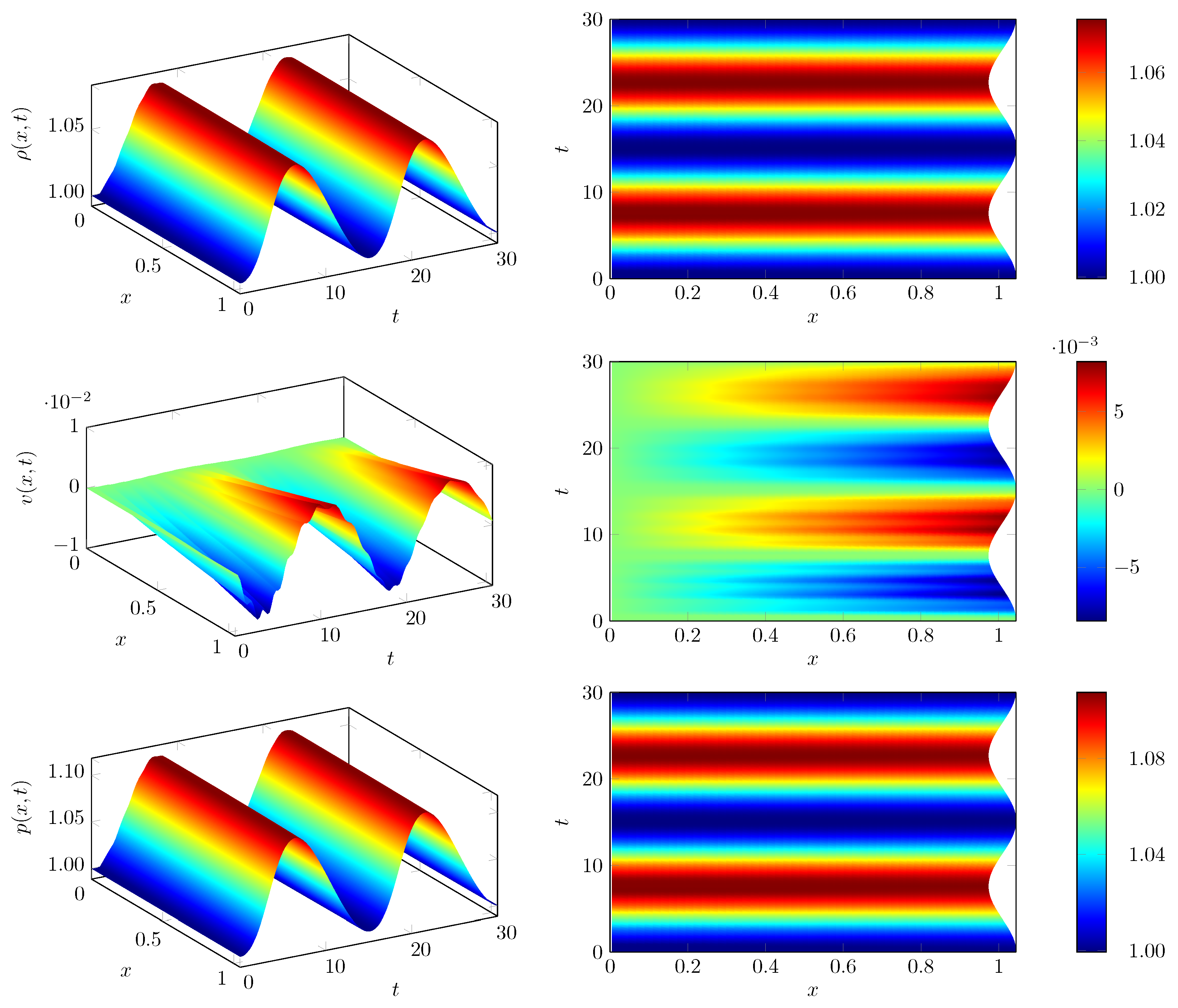
For all of our numerical tests, we initially chose an equidistant discretization of the fluid chamber consisting of 100 finite volume cells and the numerical flux function is given by the well known Lax-Friedrichs flux. The nonlinear systems of equations within the implicit stages of the RK scheme applied to the structure component (see Equation (77)) are solved using a Newton-Krylov scheme. In order to introduce non-uniformity into this test case, the deformation of the fluid domain by the piston movement is transferred to the individual grid points in a non-uniform manner. In this set-up, the spatial grid is only equidistant at those time levels where the piston achieves its initial maximal displacement. In general, the computational grid is compressed near the piston. The results depicted in Figure 7, Figure 8 and Figure 9 are obtained by adaptive determination of time step sizes for both macro and micro steps according to the strategies described in Section 3.4, i.e., solely based on embedded error control. The parameters for time adaptivity are set to , , for both micro and macro step sizes, and for the macro step sizes as well as for the micro step sizes. The simulation is carried out until the final time . Figure 7 and Figure 8 show the numerical results for the MGARK scheme based on the explicit Heun scheme for the fluid and the implicit trapezoidal rule for the structure. The coupling procedure is given by Choice B in Corollary 2. In the representations on the right hand side of Figure 7, the piston movement at the right chamber boundary is visible as well.

Figure 7.
Time evolution of density, velocity and pressure.
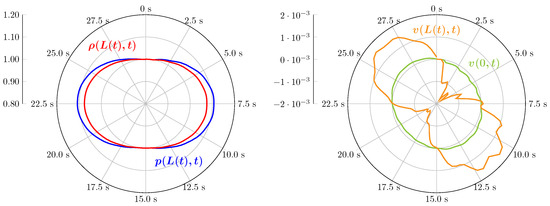
Figure 8.
Time evolution of fluid density, pressure and velocity in polar graph.

Figure 9.
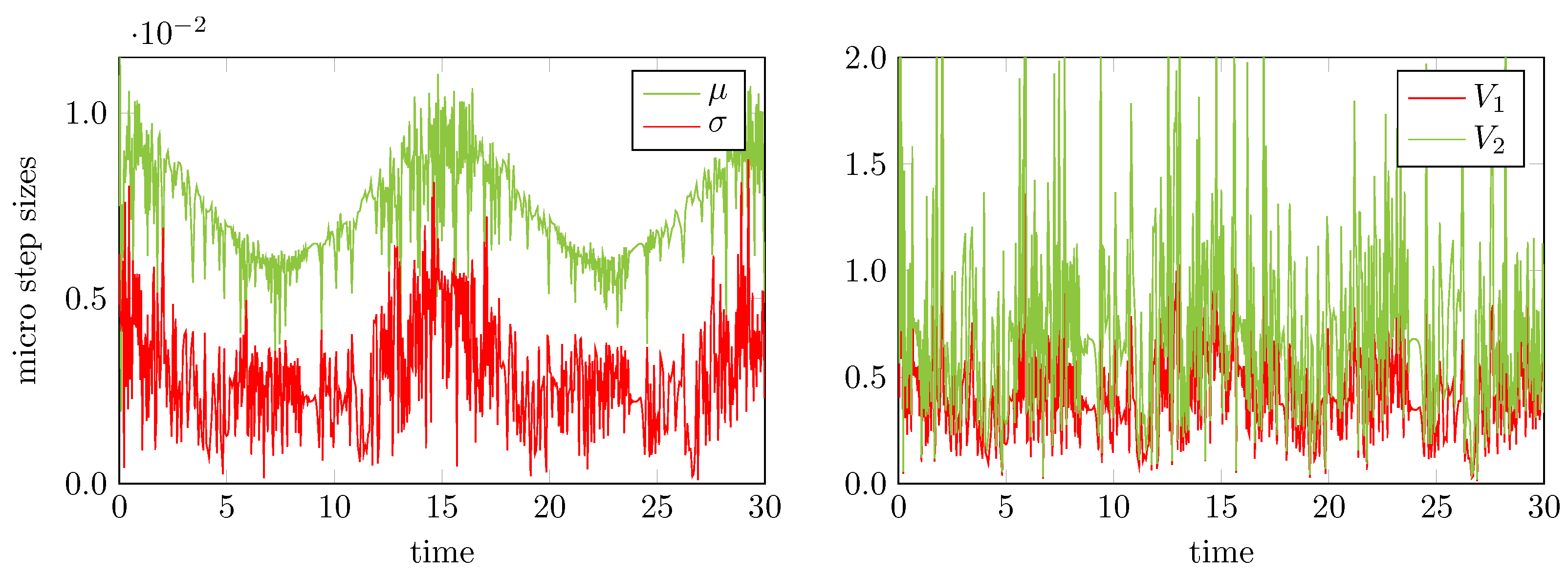
Statistics of the micro step sizes used by an error-controlled macro and micro step adaptive 2nd order multirate generalized-structure additively partitioned Runge-Kutta (MGARK) approach for solving the piston problem. Left: Mean value μ and standard deviation σ of micro step sizes; Right: Coefficients of variation.
Now we would like to pay more attention to our strategy to allow for adaptive non-constant micro step sizes within one macro step. In this regard, Figure 9 collects the statistics of the computed macro and micro step sizes. For the micro step sizes, the left part of Figure 9 shows the time evolution of the mean value μ and the standard deviation σ calculated as
for . Herein, the last micro step size of each macro step usually will be suitably shortened in order to add up to the macro step size, see Algorithm 4, line 8 and is hence not included into the calculation of the statistics. The coefficients of variation and relate the standard deviation as well as the maximum deviation to the mean value, i.e.
Hence, from these coefficients we obtain a measure of the extend of variability in relation to the mean.
As shown by the results on the right hand side of Figure 9, there are time sections with significant variability of the micro step sizes, i.e., there are sections with and sections with . Thus, the application of variable micro step sizes instead of constant ones is justified for this test case. A multirate scheme using constant micro step sizes might have used the smallest micro step size to comply with the given error tolerances which would have led to a larger amount of micro steps per macro step compared to the adaptive choice of micro steps. For the time sections with higher coefficients of variation this means a higher computational effort and thus a lower efficiency compared to the adaptive case.
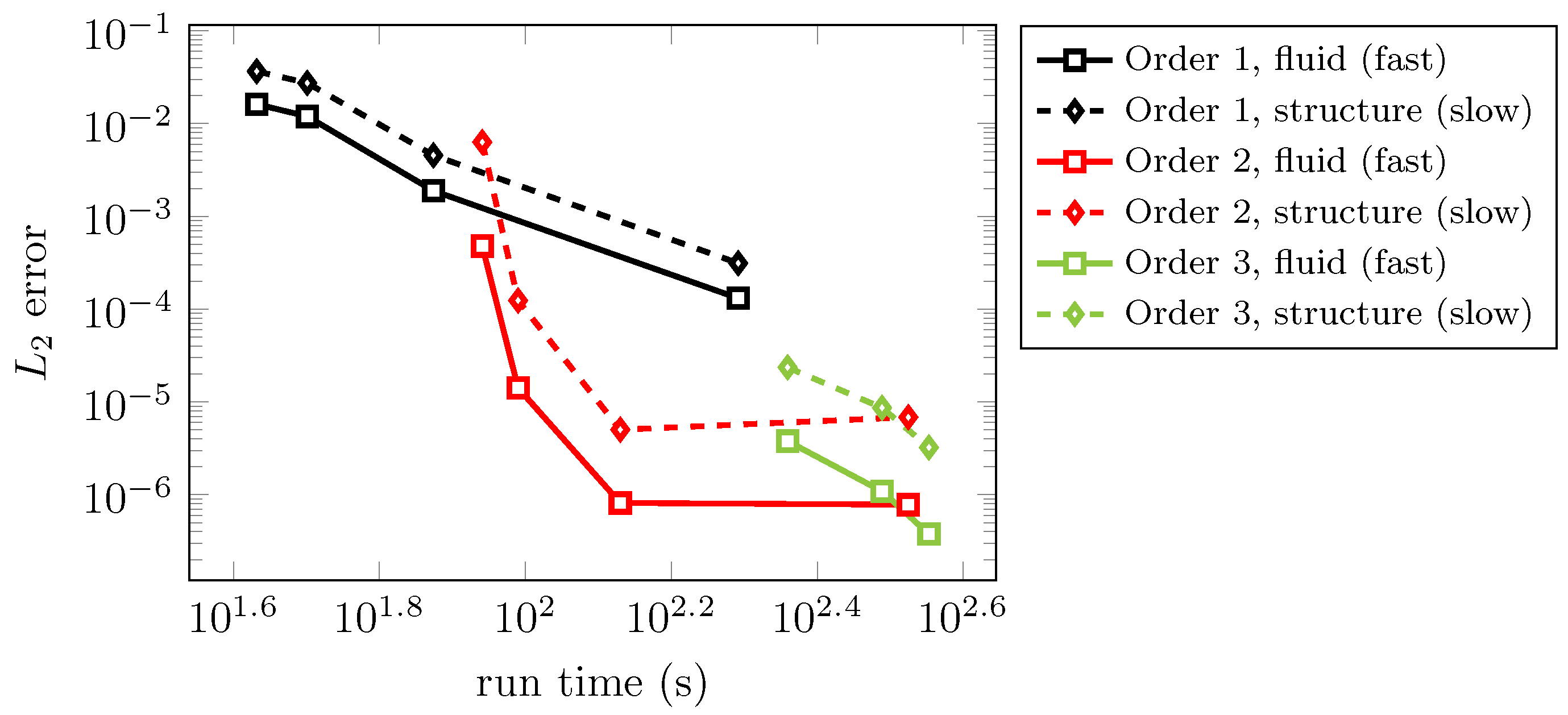
In Figure 10, an efficiency study regarding numerical error versus CPU time is depicted comparing the described MGARK schemes up to third order. Computations were carried out for the explicit Euler method coupled with the implicit Euler method and coupling coefficients set to zero (order 1), the explicit Heun scheme coupled with implicit trapezoidal scheme and second order coupling coefficients according to Corollary 2, choice B, and the IMEXRKCB3c base methods with third order coupling according to Corollary 3.
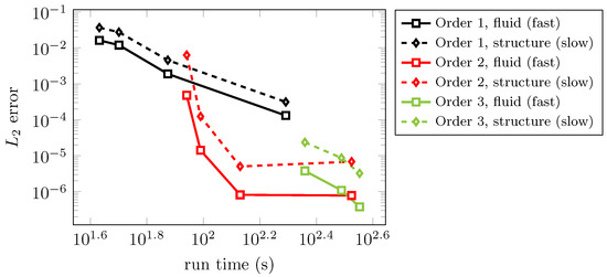
Figure 10.
Error vs. CPU time for first, second and third order MGARK scheme applied to the moving piston test case.
A spatial discretization of 100 FV cells and a final time of has been used in all test cases. The computations were carried out for different macro step sizes. During each computation, the macro step size was held constant while the micro step sizes were chosen with respect to the Courant-Friedrichs-Lewy (CFL) condition, with a CFL-number of , i.e., according the error-controlled approach described in Section 3.4. In order to compute the numerical error depicted in Figure 10, a reference solution was calculated using the 3rd order explicit IMEXRKCB3c scheme to solve the fluid–structure system as a whole in a monolithic manner with a suitably small time step size and without the use of different step sizes for the subsystems.
We remark that the reference solution is obtained on the same spatial grid as the numerical simulations. Therefore, we in fact measure the time integration error of the MGARK variants applied to the semi-discrete system which is generated by finite volume space discretization Equation (82) of first order. As the focus of this work is on time integration, we expect this to be a reasonable measure for the quality of the time integration process. Of course, the full discretization error, which may be measured with respect to a reference solution on a refined spatial grid, will be affected by both spatial discretization method and time integration scheme.
We may observe that the second order coupled time integration is most efficient for moderate to small tolerances in the range of about to . For even smaller tolerances, the third order coupled procedure starts to become efficient for this specific test case.
An efficiency study regarding run time and accuracy was carried out for the 2nd order MGARK scheme described above. The results are summarized in Table 2 and Table 3 on page 30. Again, we approximated the error using a reference solution obtained by an explicit 3rd order in time monolithic approach using a suitably small constant time step size. Within Table 2, the macro step size is denoted by H and is held constant, N denotes the number of micro steps per macro step, respectively denote the error of the fast respectively slow system component measured in norm, is the average number of micro steps per macro step in case of a micro step size adaptive approach and TOL denotes the relative and absolute tolerances in case of error-controlled adaptivity. The remaining parameters needed by error-controlled adaptivity were always set to , and for both micro and macro step sizes.
Table 2.
Comparison of run time and error of different time step adaptation strategies of the 2nd order MGARK scheme applied to the piston problem, Part I. Further explanations are given in the text.
Table 3.
Comparison of run time and error of different time step adaptation strategies of the 2nd order MGARK scheme applied to the piston problem, Part II. Further explanations are given in the text.
For the computations with an error-controlled micro step size, an initial step size of has been used. A dash indicates that the scheme diverged for the specified settings. The right part of Table 3 was computed using the minimum micro step size given by comparing the error-controlled approach to a CFL-compliant step size computation with a CFL number of 0.9.
We observe that the best error achieved with constant macro and micro step sizes is undercut by the error obtained with both of the fully-adaptive approaches (i.e., adaptive macro step sizes and adaptive micro step sizes, see Table 3) with suitably small tolerances. At the same time the fully-adaptive approaches also perform better regarding run time. In addition to the results shown in Figure 9 these results demonstrate the efficiency of our approach to time adaptive MGARK schemes and show its potential to be successfully applied to more sophisticated real-world problems.
5. Concluding Remarks
In this work, we extended the multirate GARK framework to allow for varying micro step sizes and applied the resulting coupled time integration schemes of first, second and third order to mechanical fluid–structure interaction. The computation of mesh velocities satisfying the discrete geometric conservation law is quite straightforward as long as the coefficients of the fluid base method are correctly accounted for as in Equations (59) and (60) and Algorithm 2. In case of an explicit fluid base method, demanding an internally consistent partitioned scheme requires an explicit first stage of the structure base method as well, e.g., use of an E(S)DIRK scheme. While compliance with the geometric conservation law is demonstrated for uniform flow on an artificially moving grid, we furthermore demonstrated the viability of adaptive micro steps by investigating the step size statistics for the moving piston test case. Efficiency of higher order time integration is investigated by a comparison of first, second and third order schemes in terms of error vs. CPU time where the second order coupled approach seems to be most efficient for moderate tolerances. In a comparison of various step size selection strategies, we observe a better performance of the fully-adaptive approaches choosing macro and micro step sizes based on embedded error control.
The adaptive micro step MGARK scheme could hence be an alternative to lower order coupling approaches also for more complex applications in the context of fluid–structure interaction. For this purpose, a detailed study of the stability properties of the proposed MGARK schemes is required. Corresponding studies for the given schemes as well as for alternative candidates within the MGARK framework are subject to future work.
Acknowledgments
Both authors gratefully acknowledge partial support of this study in the period of July 2014 to June 2015 provided by the German Research Foundation, SFB/TR TRR 30.
Author Contributions
Sascha Bremicker-Trübelhorn elaborated the theoretical proofs concerning the MGARK order conditions and carried out the numerical experiments in agreement with Sigrun Ortleb. Both authors jointly wrote the paper.
Conflicts of Interest
The authors declare no conflict of interest.
References
- Van Zuijlen, A.H.; Bijl, H. Implicit and Explicit Higher Order Time Integration Schemes for Structural Dynamics and Fluid-structure Interaction Computations. Comput. Struct. 2005, 83, 93–105. [Google Scholar] [CrossRef]
- Froehle, B.M.; Persson, P.O. A High-Order Implicit-Explicit Fluid-Structure Interaction Method for Flapping Flight. In Proceedings of the 21st AIAA Computational Fluid Dynamics Conference, Fluid Dynamics and Co-located Conferences, San Diego, CA, USA, 24–27 June 2013.
- Piperno, S. Simulation Numérique de Phénomènes D’interaction Fluide-Structure. Ph.D. Thesis, Ecole Nationale des Pont et Chaussées, Champs-sur-Marne, Germany, 1995. [Google Scholar]
- Piperno, S. Explicit/implicit fluid/structure staggered procedures with a structural predictor and fluid subcycling for 2D inviscid aeroelastic simulations. Int. J. Numer. Methods Fluids 1997, 25, 1207–1226. [Google Scholar] [CrossRef]
- Langer, U.; Yang, H. Robust and efficient monolithic fluid-structure-interaction solvers. Int. J. Numer. Methods Eng. 2016, 108, 303–325. [Google Scholar] [CrossRef]
- Ángel Fernández, M.; Moubachir, M. A Newton method using exact jacobians for solving fluid–structure coupling. Comput. Struct. 2005, 83, 127–142. [Google Scholar] [CrossRef]
- Küttler, U.; Wall, W.A. Fixed-point fluid–structure interaction solvers with dynamic relaxation. Comput. Mech. 2008, 43, 61–72. [Google Scholar] [CrossRef]
- Jaiman, R.; Geubelle, P.; Loth, E. Stable and Accurate Loosely-Coupled Scheme for Unsteady Fluid-Structure Interaction. In Proceedings of the 45th AIAA Aerospace Sciences Meeting and Exhibit, Reno, NV, USA, 8–11 January 2007.
- Rice, J.R. Split Runge-Kutta Method for Simultaneous Equations. J. Res. Natl. Bur. Standards 1960, 64B, 151–170. [Google Scholar] [CrossRef]
- Andrus, J.F. Numerical Solution of Systems of Ordinary Differential Equations Separated into Subsystems. SIAM J. Numer. Anal. 1979, 16, 605–611. [Google Scholar] [CrossRef]
- Engstler, C.; Lubich, C. MUR8: A multirate extension of the eighth-order Dormand-Prince method. Appl. Numer. Math. 1997, 25, 185–192. [Google Scholar] [CrossRef]
- Gear, C.W.; Wells, D.R. Multirate linear multistep methods. BIT Numer. Math. 1984, 24, 484–502. [Google Scholar] [CrossRef]
- Skelboe, S. Stability Properties of Backward Difference Multirate Formulas. Appl. Numer. Math. 1989, 5, 151–160. [Google Scholar] [CrossRef]
- Skelboe, S.; Andersen, P.U. Stability Properties of Backward Euler Multirate Formulas. SIAM J. Sci. Stat. Comput. 1989, 10, 1000–1009. [Google Scholar] [CrossRef]
- Engstler, C.; Lubich, C. Multirate extrapolation methods for differential equations with different time scales. Computing 1997, 58, 173–185. [Google Scholar] [CrossRef]
- Günther, M.; Rentrop, P. Multirate ROW methods and latency of electric circuits. Appl. Numer. Math. 1993, 13, 83–102. [Google Scholar] [CrossRef]
- Günther, M.; Rentrop, P. Partitioning and Multirate Strategies in Latent Electric Circuits. In Mathematical Modelling and Simulation of Electrical Circuits and Semiconductor Devices; Bank, R., Bulirsch, R., Gajewski, H., Merten, K., Eds.; Birkhäuser: Basel, Switzerland, 1996; pp. 33–60. [Google Scholar]
- Günther, M.; Kværnø, A.; Rentrop, P. Multirate Partitioned Runge-Kutta Methods. BIT Numer. Math. 2001, 41, 504–514. [Google Scholar] [CrossRef]
- Kværnø, A.; Rentrop, P. Low Order Multirate Runge-Kutta Methods in Electric Circuit Simulation. Available online: http://citeseerx.ist.psu.edu/viewdoc/download?doi=10.1.1.9.3084&rep=rep1&type=pdf (accessed on 1 December 2016).
- Ascher, U.M.; Ruuth, S.J.; Wetton, B.T.R. Implicit-explicit methods for time-dependent partial differential equations. SIAM J. Numer. Anal. 1995, 32, 797–823. [Google Scholar] [CrossRef]
- Knoth, O.; Wolke, R. Implicit-explicit Runge-Kutta methods for computing atmospheric reactive flow. Appl. Numer. Math. 1998, 28, 327–341. [Google Scholar] [CrossRef]
- Kennedy, A.C.; Carpenter, M.H. Additive Runge-Kutta schemes for convection-diffusion-reaction equations. Appl. Numer. Math. 2003, 44, 139–181. [Google Scholar] [CrossRef]
- Kanevsky, A.; Carpenter, M.H.; Gottlieb, D.; Hesthaven, J.S. Application of implicit–explicit high order Runge-Kutta methods to discontinuous-Galerkin schemes. J. Comput. Phys. 2007, 225, 1753–1781. [Google Scholar] [CrossRef]
- Shoeybi, M.; Svärd, M.; Ham, F.E.; Moin, P. An Adaptive Implicit-explicit Scheme for the DNS and LES of Compressible Flows on Unstructured Grids. J. Comput. Phys. 2010, 229, 5944–5965. [Google Scholar] [CrossRef]
- Sandu, A.; Günther, M. A Generalized-Structure Approach to Additive Runge-Kutta Methods. SIAM J. Numer. Anal. 2015, 53, 17–42. [Google Scholar] [CrossRef]
- Günther, M.; Sandu, A. Multirate generalized additive Runge Kutta methods. Numer. Math. 2016, 133, 497–524. [Google Scholar] [CrossRef]
- Günther, M.; Hachtel, C.; Sandu, A. Multirate GARK Schemes for Multiphysics Problems. In Scientific Computing in Electrical Engineering—SCEE 2014, Wuppertal, Germany, July 2014; Bartel, A., Clemens, M., Günther, M., ter Maten, E.J.W., Eds.; Springer: Cham, Switzerland, 2016; pp. 115–121. [Google Scholar]
- Hairer, E.; Nørsett, S.P.; Wanner, G. Solving Ordinary Differential Equations I: Nonstiff Problems, 2nd ed.; Springer: Berlin/Heidelberg, Germany; New York, NY, USA, 1993. [Google Scholar]
- Glowinski, R.; Périaux, J. Numerical Methods for Nonlinear Problem in Fluid Dynamics. In INRIA Conference on Supercomputing: State-of-the-Art; Elsevier Science Inc.: New York, NY, USA, 1987; pp. 381–479. [Google Scholar]
- Araújo, A.; Murua, A.; Sanz-Serna, J.M. Symplectic Methods Based on Decompositions. SIAM J. Numer. Anal. 1997, 34, 1926–1947. [Google Scholar] [CrossRef]
- Mavriplis, D.J.; Yang, Z. Construction of the discrete geometric conservation law for high-order time-accurate simulations on dynamic meshes. J. Comput. Phys. 2006, 213, 557–573. [Google Scholar] [CrossRef]
- Cavaglieri, D.; Bewley, T. Low-storage Implicit/Explicit Runge-Kutta Schemes for the Simulation of Stiff High-dimensional ODE Systems. J. Comput. Phys. 2015, 286, 172–193. [Google Scholar] [CrossRef]
- Lefrançois, E.; Boufflet, J.P. An Introduction to Fluid-Structure Interaction: Application to the Piston Problem. SIAM Rev. 2010, 52, 747–767. [Google Scholar] [CrossRef]
- Blom, F.J. A monolithical fluid-structure interaction algorithm applied to the piston problem. Comput. Methods Appl. Mech. Eng. 1998, 167, 369–391. [Google Scholar] [CrossRef]
- Abbas, Q.; Nordström, J. Weak Versus Strong No-Slip Boundary Conditions for the Navier-Stokes Equations. Eng. Appl. Comput. Fluid Mech. 2010, 4, 29–38. [Google Scholar] [CrossRef]
- Eliasson, P.; Eriksson, S.; Nordström, J. The Influence of Weak and Strong Solid Wall Boundary Conditions on the Convergence to Steady-State of the Navier-Stokes Equations. In Proceedings of the 19th AIAA Computational Fluid Dynamics, San Antonio, TX, USA, 22–25 June 2009.
- Nordström, J.; Eriksson, S.; Eliasson, P. Weak and strong wall boundary procedures and convergence to steady-state of the Navier–Stokes equations. J. Comput. Phys. 2012, 231, 4867–4884. [Google Scholar] [CrossRef]


© 2017 by the authors. Licensee MDPI, Basel, Switzerland. This article is an open access article distributed under the terms and conditions of the Creative Commons Attribution (CC BY) license ( http://creativecommons.org/licenses/by/4.0/).