1. Introduction
In the recent years, the research and development of unmanned vehicles have gained much attention in the academic and military communities worldwide. Systems like unmanned aircraft, underwater exploiters, satellites, and intelligent robotics are widely investigated as they have potential (dual) applications both in the military and civil domains. They are developed to be capable of working autonomously, without a human pilot. One of the main challenges is the need to deal with extremely varying situations that arise in complicated and uncertain environments, like unexpected obstacles and enemy attacks [
1].
UAV (unmanned aerial vehicles) is an acronym for a wide class of aircraft, ranging from a few centimeters to many meters in wingspan, from simple, hand-operated units to high altitude, long endurance systems similar in operation to manned aircraft. In the literature they are classified as RPA (remotely piloted aircraft), AAV (autonomous aircraft vehicles), and so on [
2,
3,
4,
5,
6]. A UAV is defined as an aerial craft, flying without human crew on-board; it can be remotely controlled or fly autonomously [
6,
7]. Over the past three decades, the popularity of UAV or UAS (unmanned aerial systems—in 2005, the U.S. Department of Defense, DoD, started defining them as “flying systems”) has kept growing at an unprecedented rate. Among different types, small-scale UAVs are gaining interest and popularity because:
They are a powerful tools for scientific research due to attractive features such as low cost, high maneuverability, and easy maintenance. Significant progress has been made in various investigation areas (e.g., dynamics modeling, flight control, guidance, and navigation);
They can be implemented in many dangerous civil applications, like emergency monitoring, victim search and rescue, aerial filming, geological survey, weather forecast, pollution assessment, fire detection, and radiation monitoring.
The development of UAVs has been strongly motivated by military applications. Indeed, their development dates back to the development of the first aerial torpedoes, almost 95 years ago. During World War I (WWI), both the Navy and the Army experimented aerial torpedoes and flying bombs. These first examples highlighted two operational problems: for instance, crews had difficulty in launching and recovering the UAV; there were several problems in stabilizing them during flight, and so on. Efforts continued through the Korean War, when military services experimented with UAV with different missions, sensors, and munitions, in attempts to provide strike and reconnaissance services to battlefield commanders.
At those times, numerous obstacles have hindered the evolution of the UAV. Firstly, technology simply was not mature enough for them to become operational. Secondly, lack of service cooperation usually led to failure. Currently, the main showstoppers include mostly non-technical issues, such as lack of service enthusiasm, overall cost effectiveness, and competition with other weapons systems (like manned aircraft, missiles, space-based assets, and so on). In this frame, small-scale UAV seem an ideal choice for collecting information with zero casualties involved [
8], at minimal implementation costs. Moreover, they seem to position into a segment with no real competitors, simply giving a novel service. They assume a unique role to warfare and defense, as for close-range surveillance and reconnaissance in confined battlefields or urban environments.
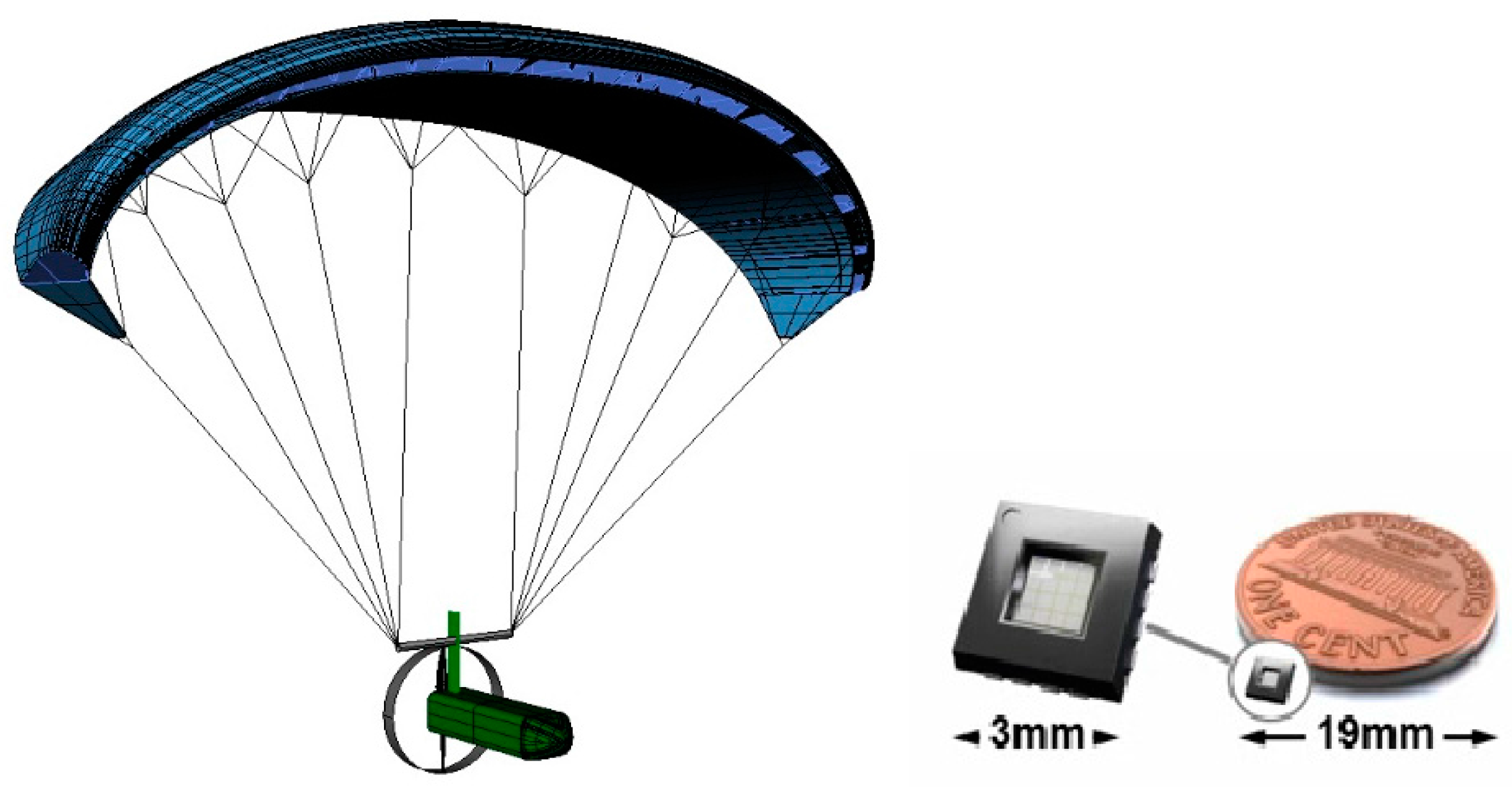
In the framework of the Military National Research Program (MNRP), and thanks to Aerosekur cooperation, CIRA (the Italian Aerospace Research Centre) has carried out a feasibility study of a small parafoil-equipped UAS for patrolling, intelligence, surveillance, reconnaissance, and telecom networking. The system is characterized by an excellent transportability and a quick configurability. Its relatively simple architecture is sketched (
Figure 1—left), where the sail and the fuselage outlines are shown. The target sensor dimensions are also reported (
Figure 1—right). The main features are summarized in
Table 1:
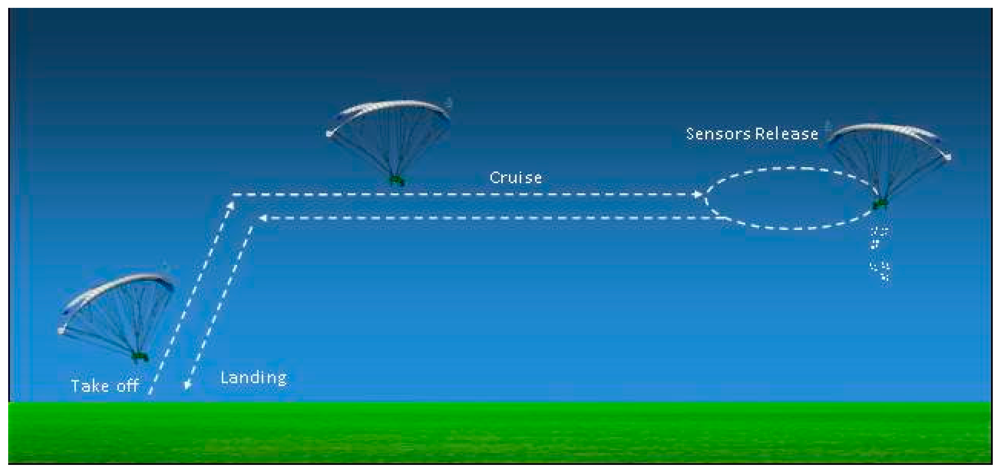
The parafoil (or “sail”) is connected to the fuselage by wires. The body hosts the flight control unit, the power supply, the engine, the payload and the landing gear system. All of the components are designed to keep the system mass and size at a minimum and to allow a compact packaging and a rapid deployment on the ground. The target vehicle is conceived to perform missions at low altitude (300 m at sea level) and limited endurance (1 h). A typical mission is sketched in
Figure 2. It can bring different payloads and sensors, depending on the selected mission (as fixed and mobile targets identification, border patrol, traffic control, and many others, also involving civil applications).
The device presented in this paper is aimed at storing and releasing sensors from the UAV. In this sense, it belongs to the robotic end effector family [
9], being in practice an interface between the UAV and the external environment. With reference to the standard classification of gripper-releasing devices (mechanical, thermo-mechanical, negative pressure, magnetic, and so on) [
10], it can be identified as a thermo-mechanical system in the sense that it is actuated through shape memory alloy (SMA), whose functioning requires heat supply. Moreover, the device was conceived to be employed for unknown environments. In fact, it is switched on during certain phases of flight, but it does not require any feedback on the status of its task.
SMAs are characterized by the co-existence of two different and distinct states or phases inside the same physical domain, namely martensite and austenite [
11]. The switch between these states may be continuous and depends on the stress and temperature levels. Microscopically, these variations are related to a re-arrangement of the crystal structure within the metal while macroscopically they give rise to relevant deformations, ranging up to several unit percentage almost reaching 10%. Together with this effect, some other material features vary, like the damping coefficient (moving from barely 1% to more than 10%) or the Young modulus (in certain cases increasing or decreasing by a factor 3—martensite to austenite, or vice versa). The reported numbers relate to NiTi-based SMA. For other compounds, those qualities may change; nevertheless, they give an idea of their strong potentiality in generating adaptive structural elements. In this article, shape memory alloys springs are used to construct a motor for deploying sensors, taking advantage of both the strain recovery (contraction) and the variable rigidity (stiffening) peculiarity. The non-linear—hysteretic nature of the SMA materials and the combined strong dependence on the applied load and temperature, make the modeling task very challenging and justify the several works focusing on the formalization of constitutive laws [
12,
13,
14] and on the empirical-experimental characterization [
15,
16].
The described system has been specifically designed to release environmental (temperature, pressure, etc.) or pollution sensors, in order to get more environmental information. In commerce, there is a quantity of such miniaturized devices, developed and applied by industry, academia and individual innovators. For instance, there are devices able to detect non-methane volatile organic compounds (NMVOC) emissions, smoke, and toxic gases, [
17]. During the mission, the UAV could work like an antenna, receiving and transmitting real-time data to a ground receiving station, or a data store, using a micro data recorder.
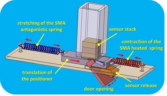
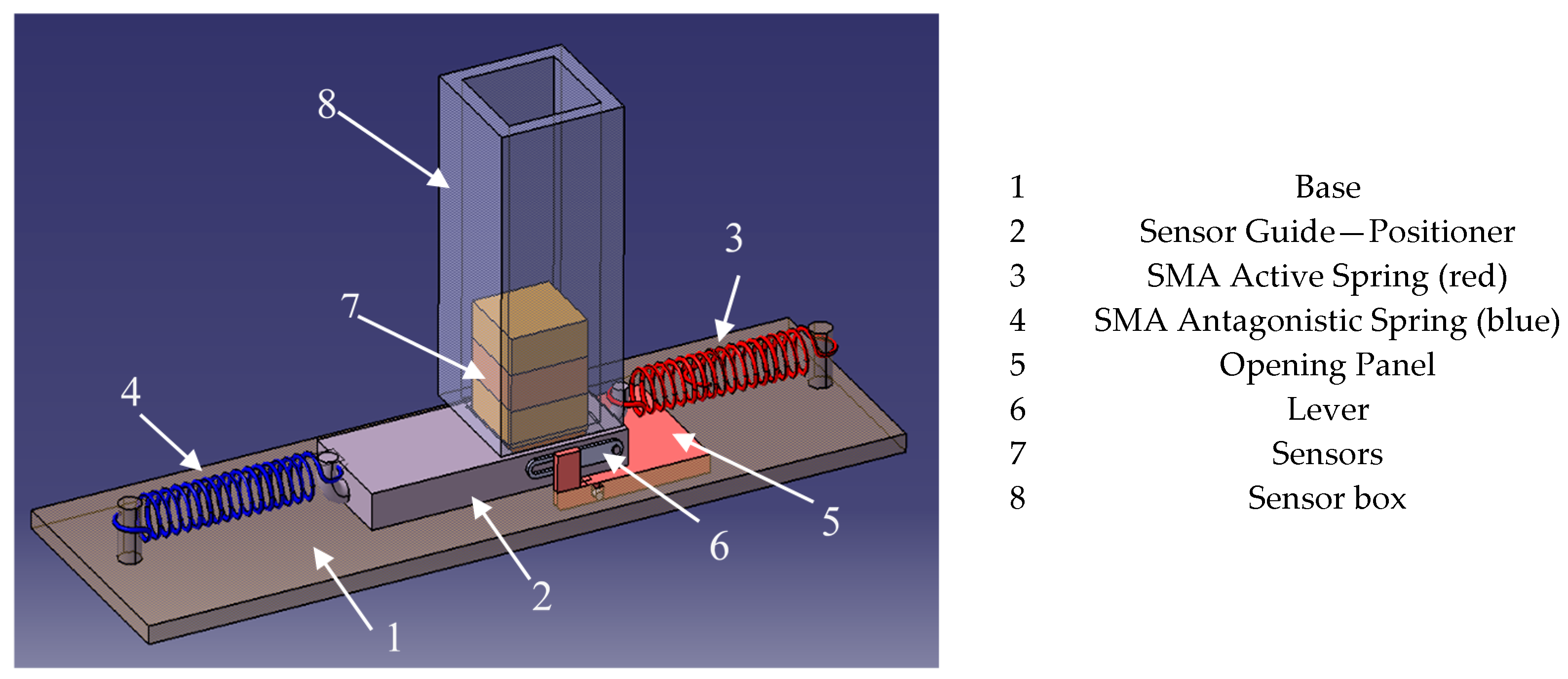
In order to give the UAS some further capability, a simple, affordable, low-cost deployment system was specified. This paper deals with the design of an environmental sensor spreader (ESS). The concept is shown in
Figure 3. It is made of a bottom door, an SMA-based sensor mover and a kinematic chain, devoted to ensure the due synchronization between the movement of the different elements and in particular the panel opening (from which the sensor is launched to the ground) and the settler displacement (that pushes the sensor to the door).
SMA actuators permit a strong reduction of the system parts and, then, its complexity. In similar applications, a servo actuator opens the panel [
18,
19], while another servo actuator grips and releases the objects [
20,
21]. The use of a bulk SMA component simplifies the overall architecture. The penalty that shall be paid for the related efficiency reduction (1 to 5) is well compensated by the decrease in the number of pieces (a good index for reliability and maintenance), weight savings, and compactness. This advantage can be also exploited for other on-board components like landing gears, deployable antennas and others [
22,
23,
24,
25,
26,
27,
28,
29,
30,
31].
Different aspects, like the power supply, the weight, the size, and the maintenance, play critical roles and must be carefully taken into account from the early stage of the design of this specific end effector. The application of SMA actuators offers some advantages, proved by several studies and patents [
32,
33,
34,
35], ranging from the industrial [
36], to the medical-surgery [
37], the aerospace [
38], and the automotive [
39], fields. The compactness and the high energy density favor lighter and solid design solutions for instance compliant with the typical aerospace weight and maintenance requirements [
40]. The large transmittable forces and displacements well meet often conflicting desiderata, like grasp and deployment specifications, typical of hand-like grippers [
32]. The possibility of tuning the electrical signal, used for the SMA heating, makes available a signal for a feedback control, applicable in the low frequency bandwidth [
41].
On the other hand, some general drawbacks and limitations must be necessarily considered. The low mechanical efficiency may limit the use of those actuator systems to small applications [
40]; the thermal inertia of the material may exclude any dynamic application (practically, ≥2 Hz); the electrical supply imposes the use of adequate thermal and electrical insulation strategies.
All of these aspects were taken into account during the early stage of the device design. In compliance with the drafted characteristics, the SMA actuators size (here used in the form of springs) were contained. The kinematic chain in charge of opening the panel and moving and dropping the sensor was optimized to assure an adequate movement synchronization and to guarantee a global simplification of the overall system architecture. Finally, the springs were supposed to be directly in contact with the calm air contained within the fuselage volume and, thus, in natural convection regime. Force convection strategies would speed up the cooling process, making the release task faster, but would also penalize the system in terms of power consumption (keeping the springs at a lower temperature). Numerical and empirical investigations aimed at enhancing the cooling process through inlets/outlets will be considered in future works with the scope of optimizing the system for specific missions and enhancing the technology readiness level (TRL).
The device development started from an investigation about its functionality, based on geometrical considerations and multi-body simulations. The model reproduced both the positioner translation and the door rotation. A concentrated force simulated the action of an active SMA spring working against an antagonistic SMA spring, whose reaction was estimated through the classic force-displacement curve, experimentally determined. This empirical approach was considered applicable to the device conceptual design task, while more sophisticated models (Finite Element, FE, integrated with dedicated constitutive laws [
42,
43]) will be taken into account for future works, focusing on the optimization of the different functional parameters. By correlating the active spring displacement to the door rotation, the kinematic frame was set. The force, necessary to achieve a certain configuration, was calculated by imposing the energy balance between the elastic energy stored in the antagonistic spring and the work done by the external actions (i.e., the active spring force and the sensors weight moment, evaluated with respect to the door pivot). Numerical simulations were related to experimental results, obtained through a test campaign on a functional mock-up (
Figure 3). The experiments allowed validating the theoretical model and verifying the system functionality; moreover, they permitted drafting a preliminary relationship between the SMA activation temperatures and the system kinematics. Finally, the achieved performance was compared to the original requirements.
3. Working Principle of the Environmental Sensor Spreader (ESS)
The equilibrium state between the two SMA springs, in turn modulated by their excitation levels, creates a certain ESS system configuration. Its mechanics follows these steps:
Step 1—“Initiation”: In this phase, the two SMA springs are in a pure elastic equilibrium (there is no activation by any external source). At their installation, the springs are stretched and connected each other, thus achieving the pre-load equilibrium. Their stretching induces the transformation of the initial full austenite into martensite. To this aim, a material was selected, characterized by a martensite start temperature (Ms) very close to the specific environmental conditions. Therefore, the necessary stress increment to induce the desired transformation may be kept at a minimum. On the other hand, it should be mentioned that this limit cannot be fully approached in order to avoid the insurgence of non-commended activations due, for instance, to a hot sunny day.
The martensite fraction, ξ, produced during the stretching can be expressed as a function of the curvilinear abscissa along the experimental black curve in
Figure 5. There, it shows the force-displacement history the springs undergo when they are integrated into the system. The initial linear slope of the curve corresponds to a classical material behavior, regulated by the austenite Young modulus. As the applied load arises, the gradual transformation into martensite occurs. The transformation process may continue up the phase transformation is completed. In the graph, this is evidenced by a relevant change of the line angle, characteristic of this transitional effect. The higher the martensite fraction in the pre-load condition, the wider the recoverable displacement through the activation. In the pre-load condition, the sensor is ready in the dispenser (guide-positioner,
Figure 6—top). Considering the relation among the rigidity,
K, of the springs and the wire diameter,
di, the winding diameter,
D, the number of windings,
N, and the shear modulus,
G:
and adapting the shear—normal elastic moduli relation to the ξ weighted average of the martensite,
Em, and austenite,
Ea, Young moduli:
An estimate of the martensite fraction can be obtained at each point of the curve. In particular, ξ results equal to the 85.5% in pre-load condition. This verification was experimentally performed by releasing the spring after having reached the target elongation. It moves then along a straight line, the slope of which is related to “K”, Equation (1). By using the Equations (1) and (2), an estimate of the effectively achieved ξ is easily produced.
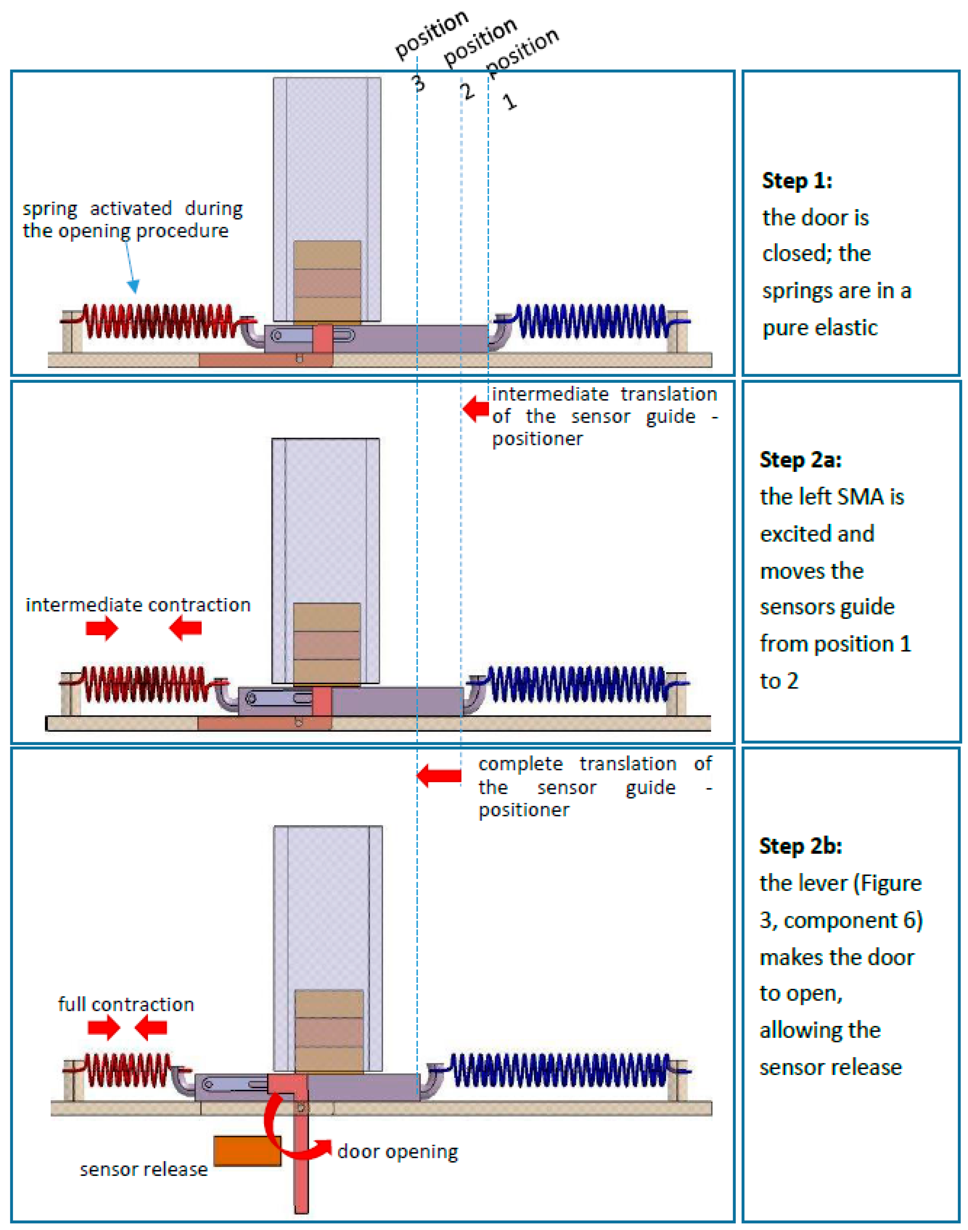
Step 2—“Door opening”: It is made of two coordinated movements: a translation of the sensors guide coupled to a rotation of the ejection panel. In particular:
At first, the active SMA spring (red in
Figure 6) is excited and pulls the sensors guide from position 1 to 2 (
Figure 6—middle);
At position 2, while the sensor guide continues its movement, a lever system (
Figure 3, component (6) opens the door and allows releasing the sensor (position 3,
Figure 6—bottom).
Step 3—“Door closing”: Once the sensor is dropped, the active SMA spring excitation is turned off and the antagonist elastic element (blue) returns the system in its original configuration; the process may be accelerated by activating this other spring, in turn. The switch rail is driving backward to close the door.
4. Modeling
The system was modelled according to the schematic reported in
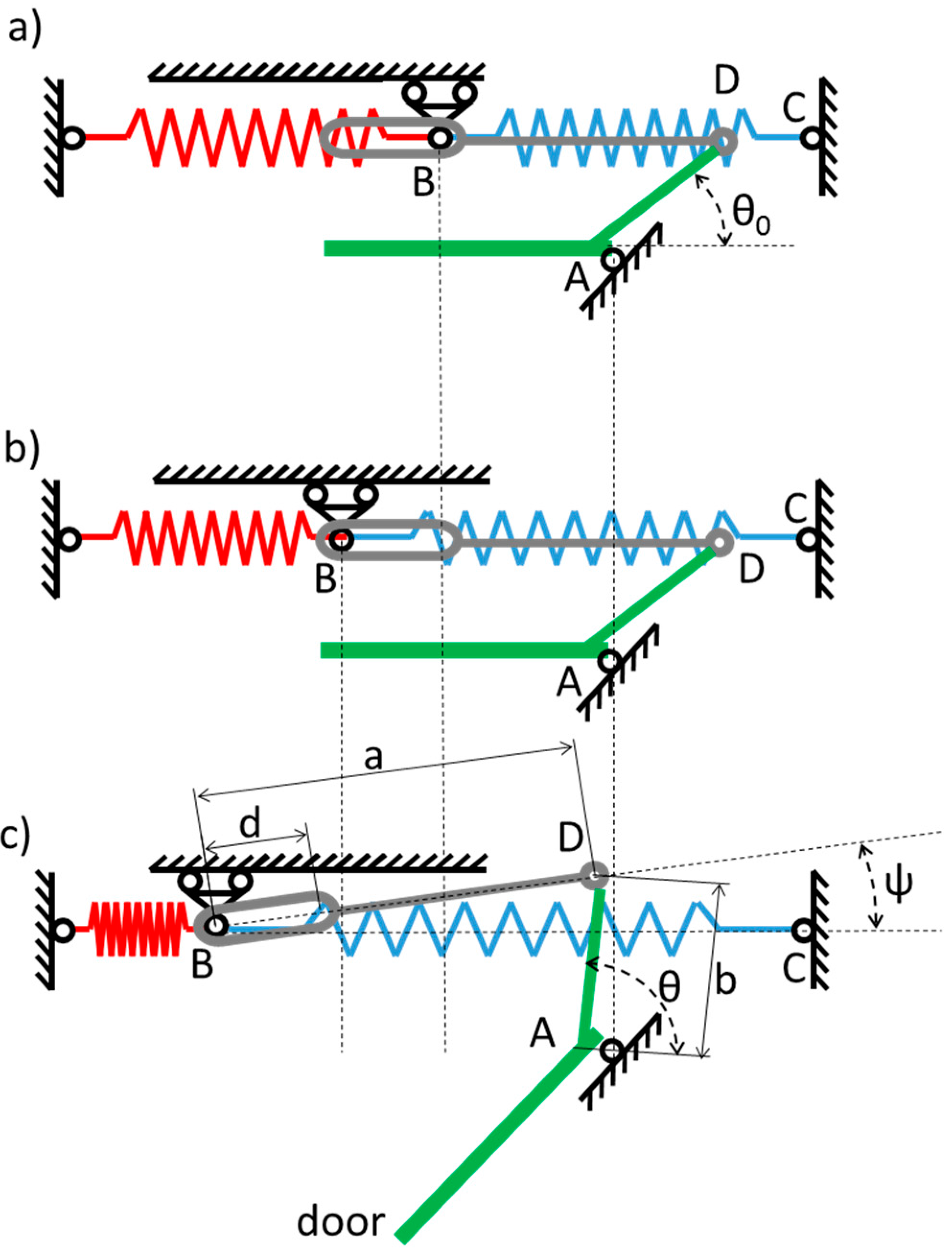
Figure 7. Therein, the “active” red and the “antagonistic” blue springs are shown as a joint in B. The positioner is not sketched; it is linked to the two elastic elements through the point B. As the red spring contracts, it moves to the left, within a slide (grey in the picture). The green segment AD represents a lever that is rigidly connected to the door, schematized as a further green line from A to the left. This couple is hinged in A, so that a motion of the point D causes its rotation. The first picture, (a), represents the initial state of the system: a closed door, non-excited and equilibrated springs, with point B at the right slide endpoint.
The activation of the red spring produces an initial translation of the point B, which moves to the left slide endpoint (
Figure 7b). Since this moment, a further contraction of the red spring forces the motion of the slide to the left; as it is rigidly connected to the point D (grey line), this causes a rotation of the lever (segment AD) and the door (
Figure 7c). It is important to remark that the blue spring and the grey connection are not interfering each other; they are just overlapped in the 1D drawing but they have no point in common. The movement may continue until the left spring reaches its max contraction. A block did, however, limit the door rotation at 75° from the initial value θ
0, following the specifications. In
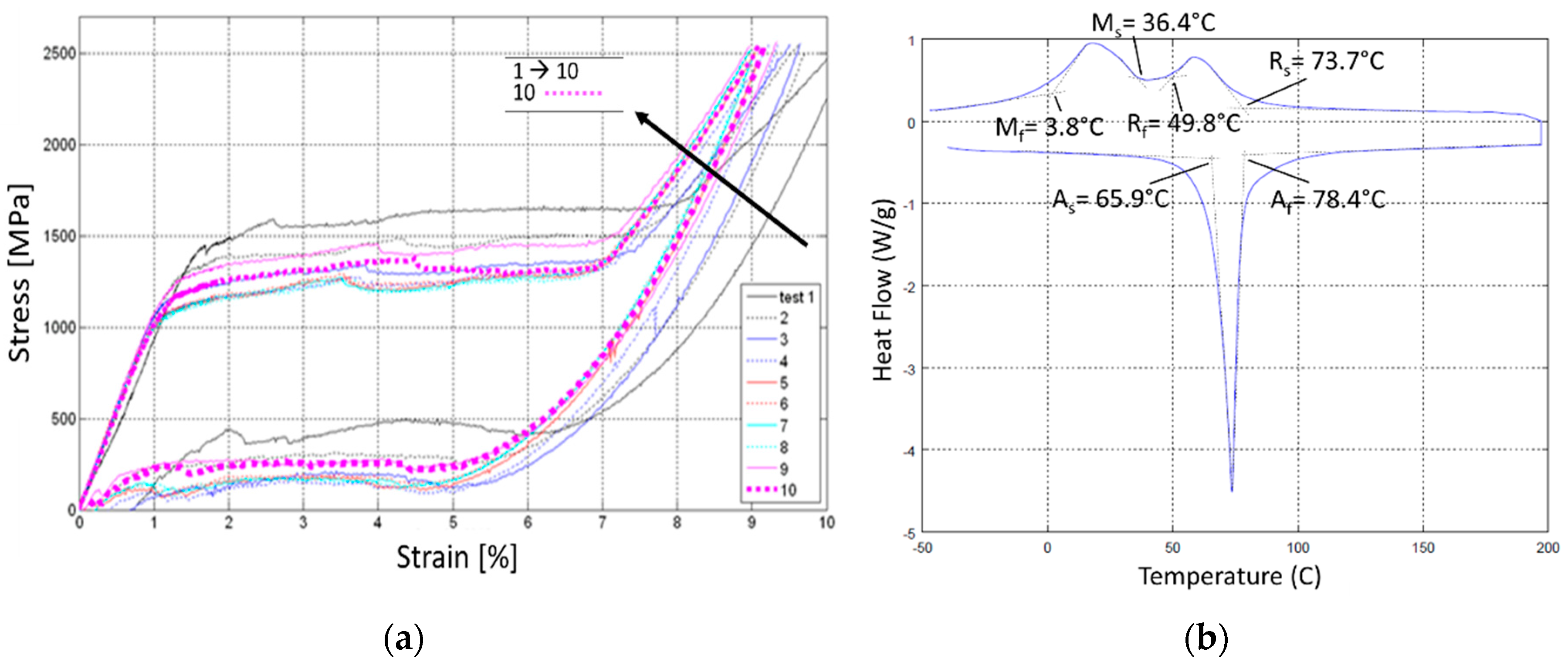
Table 2 and
Table 3, the main SMA spring parameters and the main overall system features are reported, in order. The selected NiTiNol alloy (Ni 49.8%) was experimentally characterized. Austenite and martensite Young moduli were determined through tensile tests and Differential Scanning Calorimetry, DSC, measurements at “0” load condition after the necessary stabilization cycles. The material underwent tens of mechanical cycles at room temperature (23 °C), and the last most significant cycles, in terms of convergence, are plotted in
Figure 8a.
The modelling started with the formalization of the non-linear relation between the door rotation, θ–θ
0 (respectively, current and initial angles between the lever AC and the ground line), and the point B translation. These are the main descriptors of the kinematic chain. For displacements that were lower than the slide length,
d,
Figure 7b, the angle was kept constant at θ
0 (closed door). For displacements larger than
d, a trial value is used to start the iteration to assess the running angle. The equation linking ψ, the angle between the slide and the ground line, and θ can be written as:
In the above formula,
b,
a, and
h represent the length of the segments AD (lever), BD (slider system), and the vertical distance between the point C and A, respectively. The relation between the longitudinal displacement of the point B,
xB, and the angle θ is, instead:
The sign of the estimated residual,
R, derives from the bisection method that generates a further value for θ used again in Equations (3) and (4) until convergence occurs (R ➜ 0). The resulting rotation—displacement curve is reported in
Figure 9, for θ ranging between 0° and 90°. Spring displacement is plotted with respect to its equilibrium length (zero displacement corresponds then to
x = 54 mm). A circular marker highlights this state in the picture. Moving from this point, displacements of B do not produce any rotation until they are lower than
d. After that, the door starts opening and the curve leaves the x axis. The spring activation force was computed by expressing the system energy balance, Equation (5). It takes into account the elastic energy stored in the antagonistic spring, left side, the active spring work, first term on the right side, and the work performed by the door weight momentum around A, second term on the right side:
In the equation above, W and rcg are the door weight and the distance of its center of gravity from the pivot, in order. The cosine function expresses the variation of the weight momentum arm with respect to A, as the door rotates. Fact represents the activation force, unknown, while Fantag relates the displacement of the antagonistic spring to its reaction. This relation between the applied force and the induced displacement is experimentally determined by measuring the spring displacement caused by different loads.
Equation (5) can be numerically solved for
Fact, in order to relate this parameter to the induced displacement,
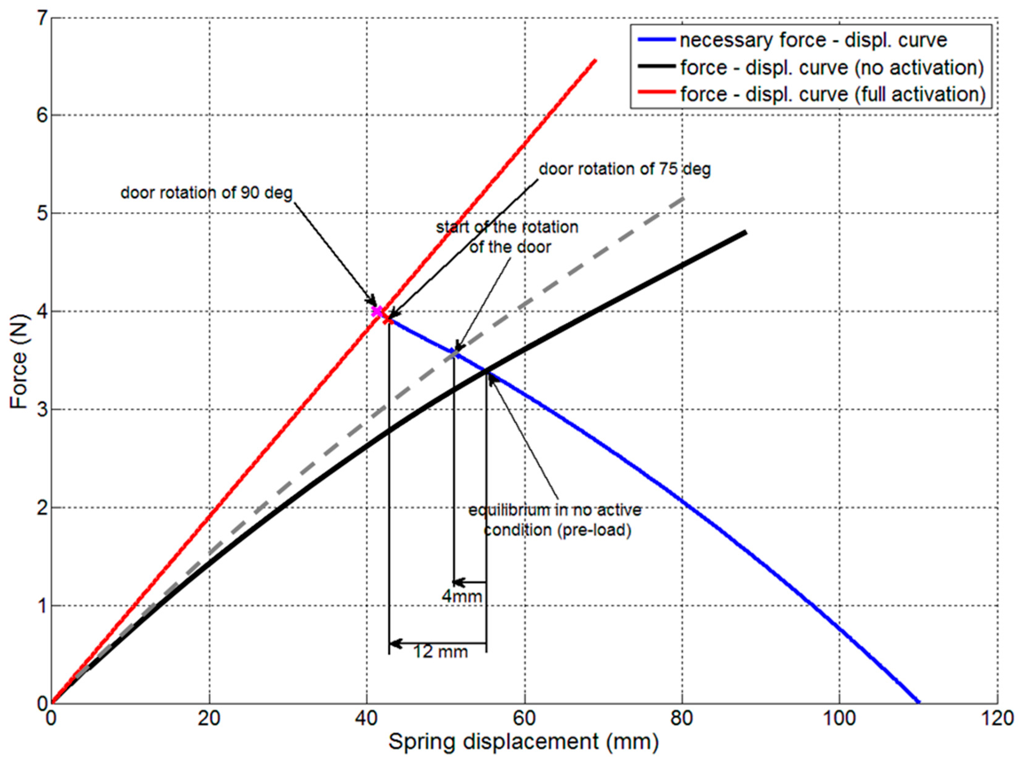
xB. The characteristic system working points (representing the non-activated and the fully-activated states) can be found by displaying three different curves onto a single graph,
Figure 5:
The just-mentioned “Fact-xB” curve (blue);
The force displacement curve (black) for the non-activated SMA spring; this curve was plotted at the environmental temperature, Tenv: as the load rises, the transformation into martensite is enforced;
The force displacement curve (red) for the fully activated SMA spring; this curve refers to a pure austenite phase and it was plotted under the assumption the temperature was sufficiently high to keep pure the austenite condition within the entire load range.
Moving from the pre-load point on the black curve (“equilibrium in no load condition”), any rise of the SMA temperature enforces its transformation into austenite, passing through intermediate configurations, like the one depicted by the grey dashed curve. The intersections between the blue and these curves represent initial and final equilibrium points of the global system. Since the pre-load condition is located on the constant slope part of the black curve, it is possible to assume that the spring works, moving from a full martensite condition. Full activation may lead to an 85° door rotation, well larger than the required one (75°). The device then has good operational margins.
The selected configuration allowed a remarkable simplification of the overall modelling process. In fact, once the two-spring system has been brought to its equilibrium state, the working philosophy moves the operational point up and down along the blue curve that is reported in
Figure 5 and was experimentally determined (indeed, the things are a bit more complex as will be explained below). The active spring cycles between a partial martensite (point
A,
Figure 10) and a full austenite state as its temperature grows (point
B,
Figure 10). At the cooling, the active spring mutates again and comes back to a partial martensite phase.
This description is strictly valid if a classical antagonistic elastic spring is considered. Since this last element is also made of the same shape memory alloy, after having moved from the initial point
A to the working point
B, the forced reverse transformation does not occur according to the blue curve,
Figure 5. Instead, because austenite is created, the return happens along a different, more inclined slope,
Figure 10 (
B ➜
C). As this other component cools, however, the working point moves up again to the initial one (
C ➜
A).
Furthermore, the segments
BC and
CA should not be considered as straight, but as part of curves, characteristic of the SMA change of phase. This takes place in theory. In the practical application, from one side the two segments are practically coincident and, on the other side, this event does not add any particular information. Then, for the scope of the present work, this behavior complication may be neglected (i.e., segments
AB and
BC are hardly distinguished and may be considered straight) and the system may be described by the curves already illustrated in
Figure 5.
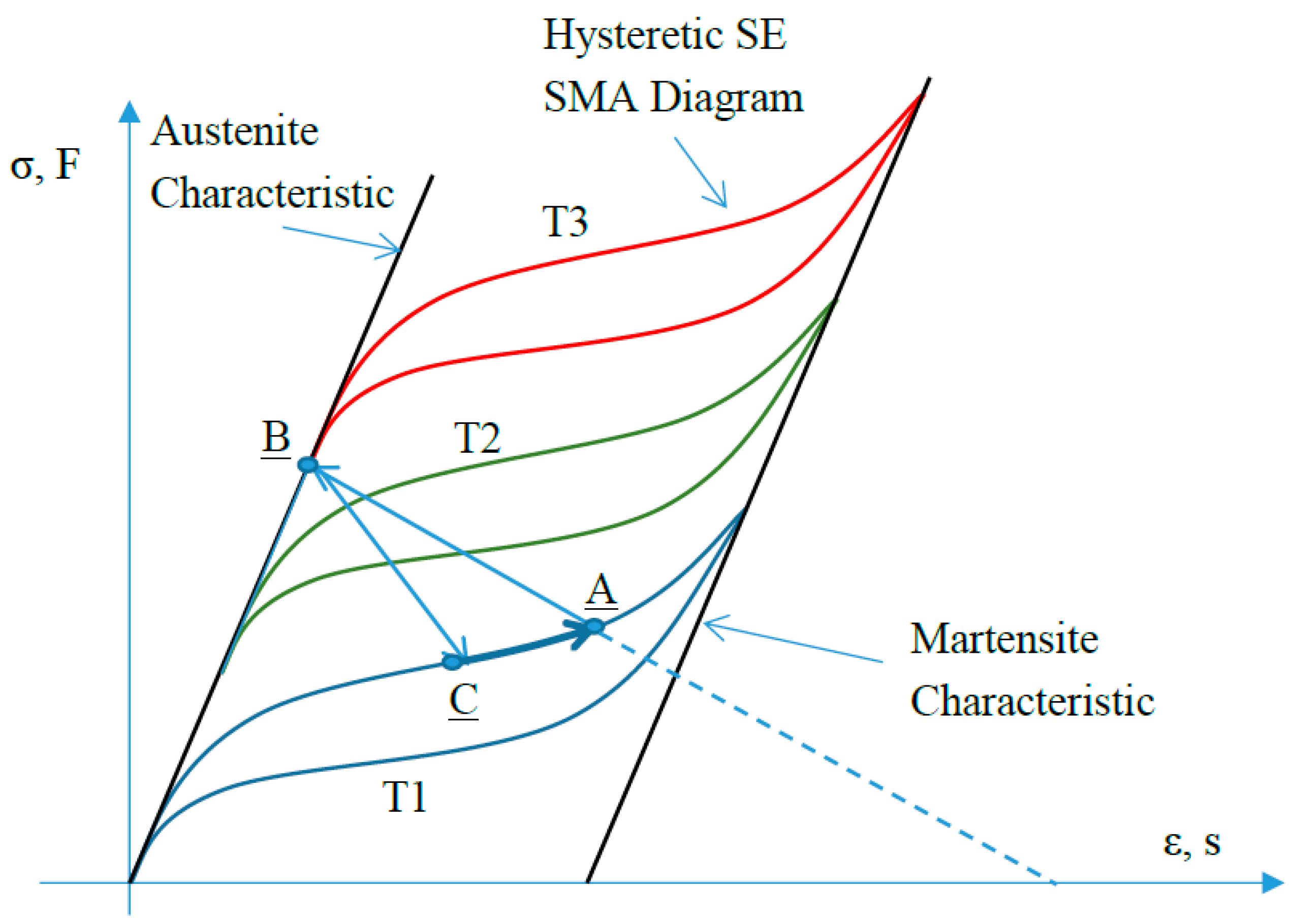
For the reader’s benefit, an ordinated description of
Figure 10 is reported. The equilibrium state,
A, is reached at temperature T1. The active spring is then warmed to temperature T3 (T2 is an intermediate value). The working point then moves from
A to
B. When the active spring is cooled and the antagonistic spring is excited, the working point moves from
B to
C, according to the partial to full austenitic characteristic (curve
BC). As the antagonistic spring also cools, the working point again approaches the original point
A. AB and
BC are not namely straight lines but they are represented in that way for the sake of clarity.
5. Manufacture and Test
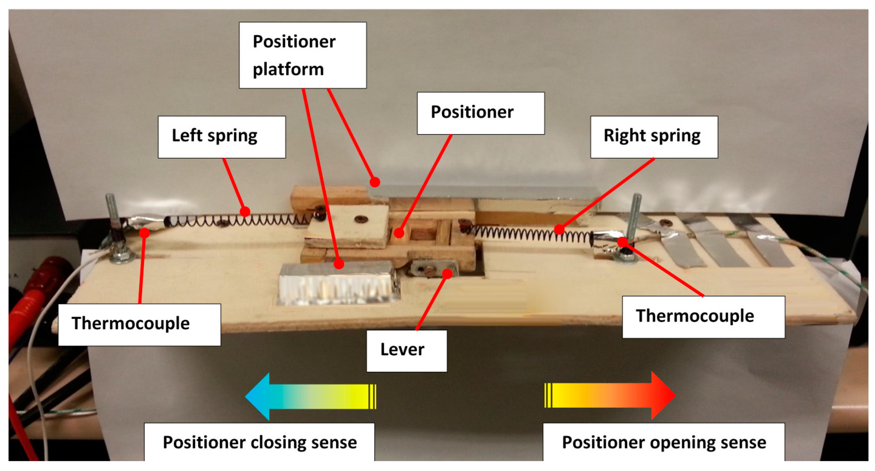
A conceptual prototype was then realized (
Figure 11). A dedicated experimental campaign was organized with the double aim of appreciating the real system ability in deploying the sensors and monitoring the main device parameters like the spring temperature and displacement, the door rotation, the supplied energy, and so on. In particular, two different test campaigns were performed:
Functionality tests, aimed at verifying the system operation;
Monitoring tests, for characterizing the device state and correlating the various descriptors.
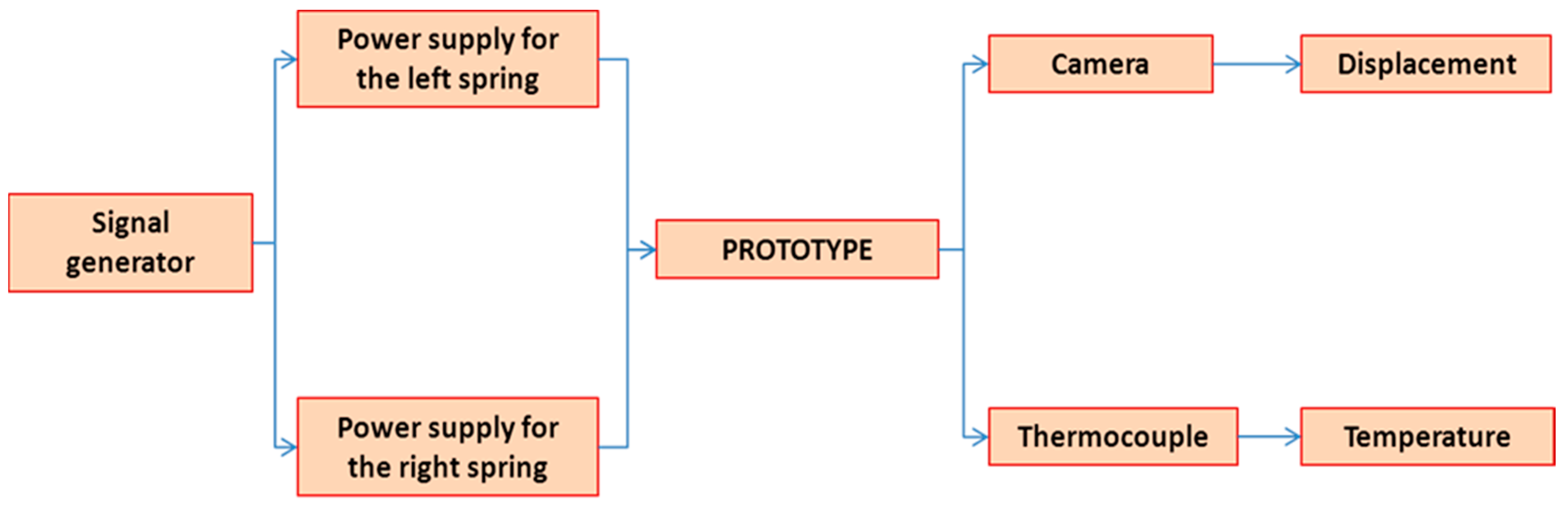
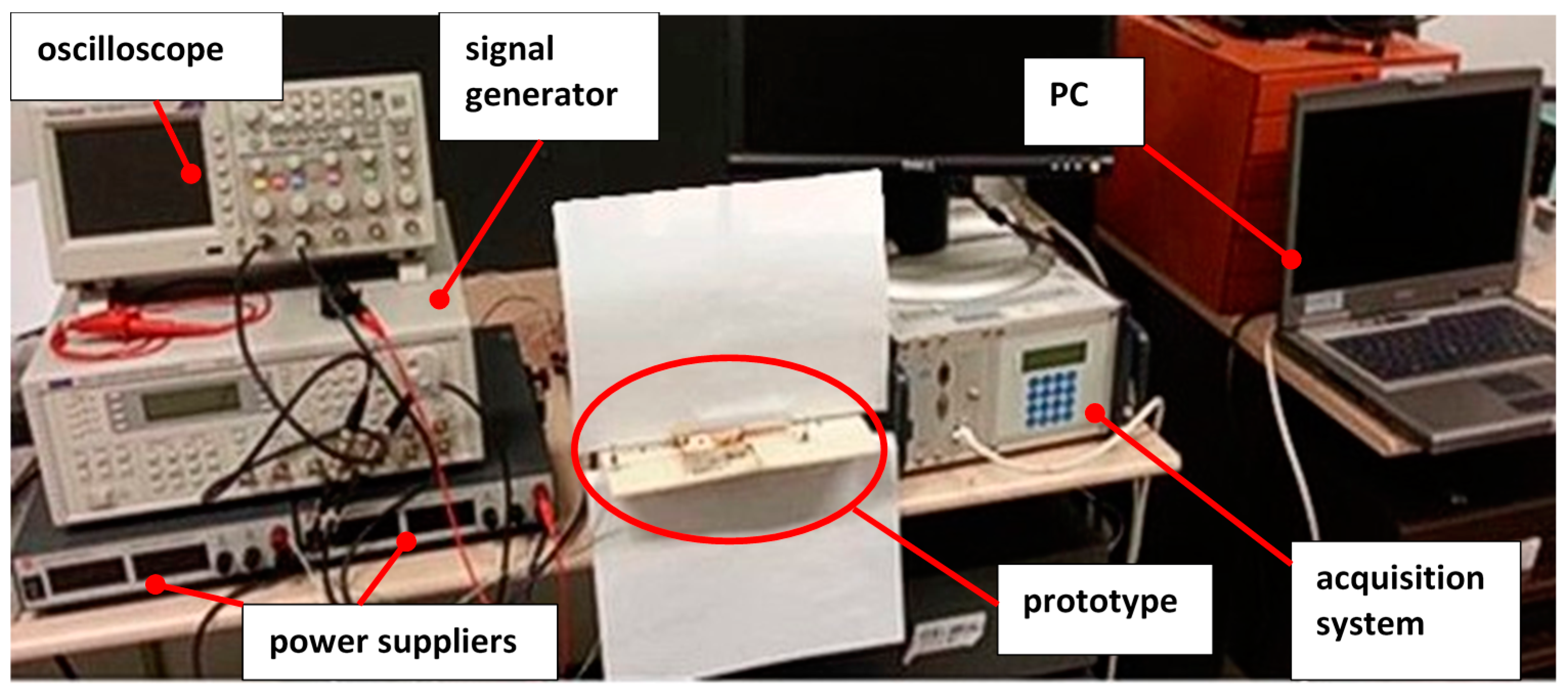
Pictures of the setup block diagram and the experimental setup are shown in
Figure 12 and
Figure 13, respectively. The following instrumentation was used:
The prototype of the sensor release system,
Figure 11, clamped on a supporting structure;
A four channel, 24 MHz signal generator, for the generation of the logical signals, necessary to drive the power suppliers that fed the SMA springs;
Two power supplies, operating within 0–30 V and 0–10 A current ranges;
An oscilloscope, dedicated to monitor the driving logical signals;
An acquisition system, to manage and store the output analogic signals (50 ms sample rate);
Two “K-type” thermocouples;
A digital camera to take pictures of the system, during the experiments.
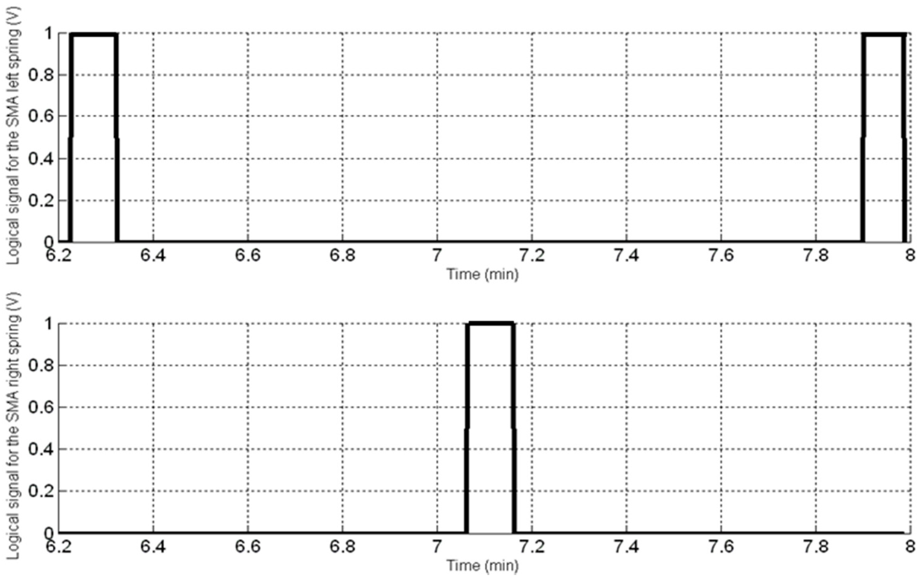
Both the functionality and the monitoring tests were performed by activating both of the springs, alternately. The operations were structured as follows. Two anti-phase logical step signals were produced to drive the active and antagonistic springs, separately. The two power suppliers were then activated in turn (
Figure 14). Each complete cycle (activation—deactivation) took 100 s and the springs were heated for 5 s. The power supplies provided a current of 2.5 A under a voltage of 1.2 V, corresponding to 3 W per spring (Direct Current, DC).
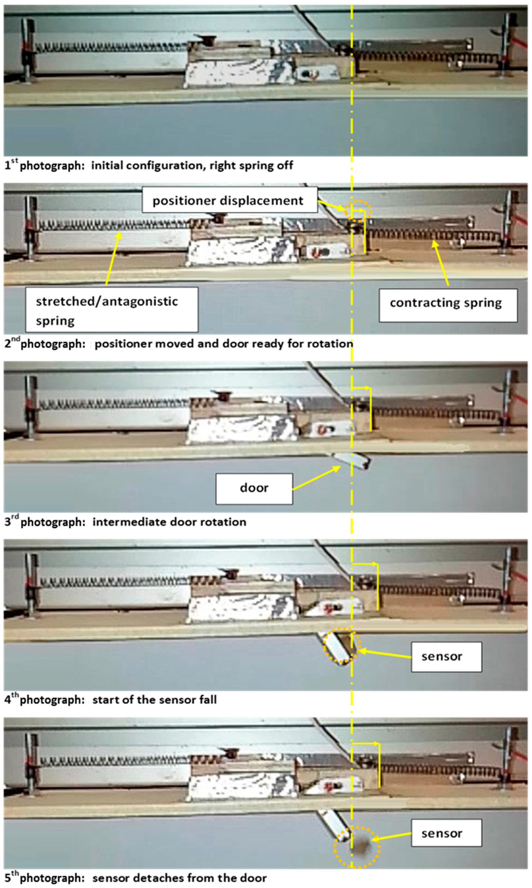
An example of the performed functionality tests is shown in
Figure 15. Therein, a sequence of video shots details the door opening and the sensor release. At first, the sensor moves horizontally, pushed by the positioner (first frame: start of the cycle; second frame: positioner moved and door ready for rotation). Then, the door starts opening (third and fourth frames: intermediate door rotation and start of the sensor drop). Finally, the sensor is released (fifth frame). The system operability was then proved. The vertical dashed line indicates the initial location of the positioner. A system characterization was then carried out for evaluating the main working parameters. The system was driven for several cycles. Two thermocouples monitored the spring temperature, while the camera captured different states of the working device. In
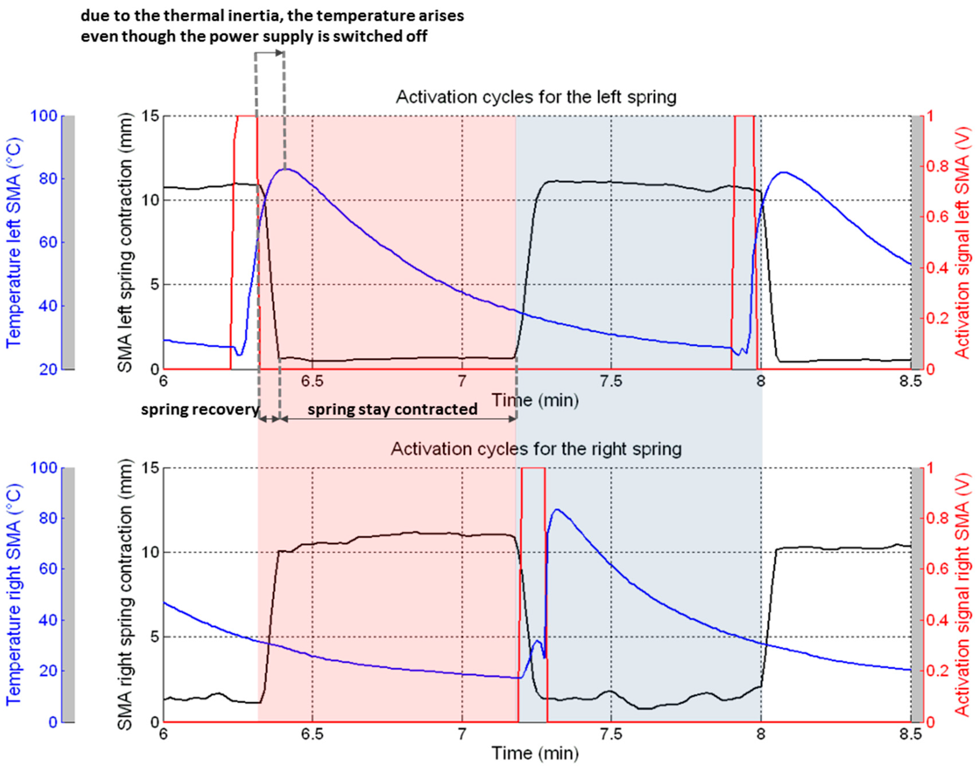
Figure 16, the activation signal, the temperature and the corresponding displacement are plotted along a complete activation-deactivation cycle for both the SMA elements over a period of 1.8 min.
The complete operation may be divided into two segments, each 0.9 min long. The first is related to the contraction of the left spring and its following subsequent freezing in this condition (door opening—pink area); the second refers instead to the contraction of the antagonistic SMA that brings the device back to the initial configuration (door closing—light blue area). In detail, the temperature of the left spring arises from the environmental condition up to 82 °C (
Figure 16—top). A certain inertia of the power supply could be observed for around 6 s, since the spring temperature continued growing even after it was switched off (dashed vertical lines,
Figure 16—top). The contraction started at the early supply start, as shown by the corresponding displacement curve (black): from 6.30 to 6.35 min, the length of the left spring passed from 10.1 to 1.0 mm. A specular behavior was observed for the right elastic element,
Figure 16—bottom, since they are connected to each other and as the one shrinks, the other stretches.
The sensor release is accomplished as the active SMA fully shrivels (“spring recovery” label,
Figure 16—top). Then, it remains for a while in this configuration, as indicated by the “spring stay contracted” label, up to the end of the pink area. In this phase, the door stays open while the active spring cools in a natural convection regime. When it reaches 40 °C the antagonistic device is activated. This temperature was considered a good compromise between two opposite requirements. The necessity of starting the deactivation cycle as soon as possible demanded a rapid activation of the other element to reverse the process. On the other hand, the lower the austenite percentage is within the left spring (and, thus, its temperature), the lower is the force, necessary to reset the system. In this second phase, the door closes and the positioner moves back. At this point, the system is ready for another operation.
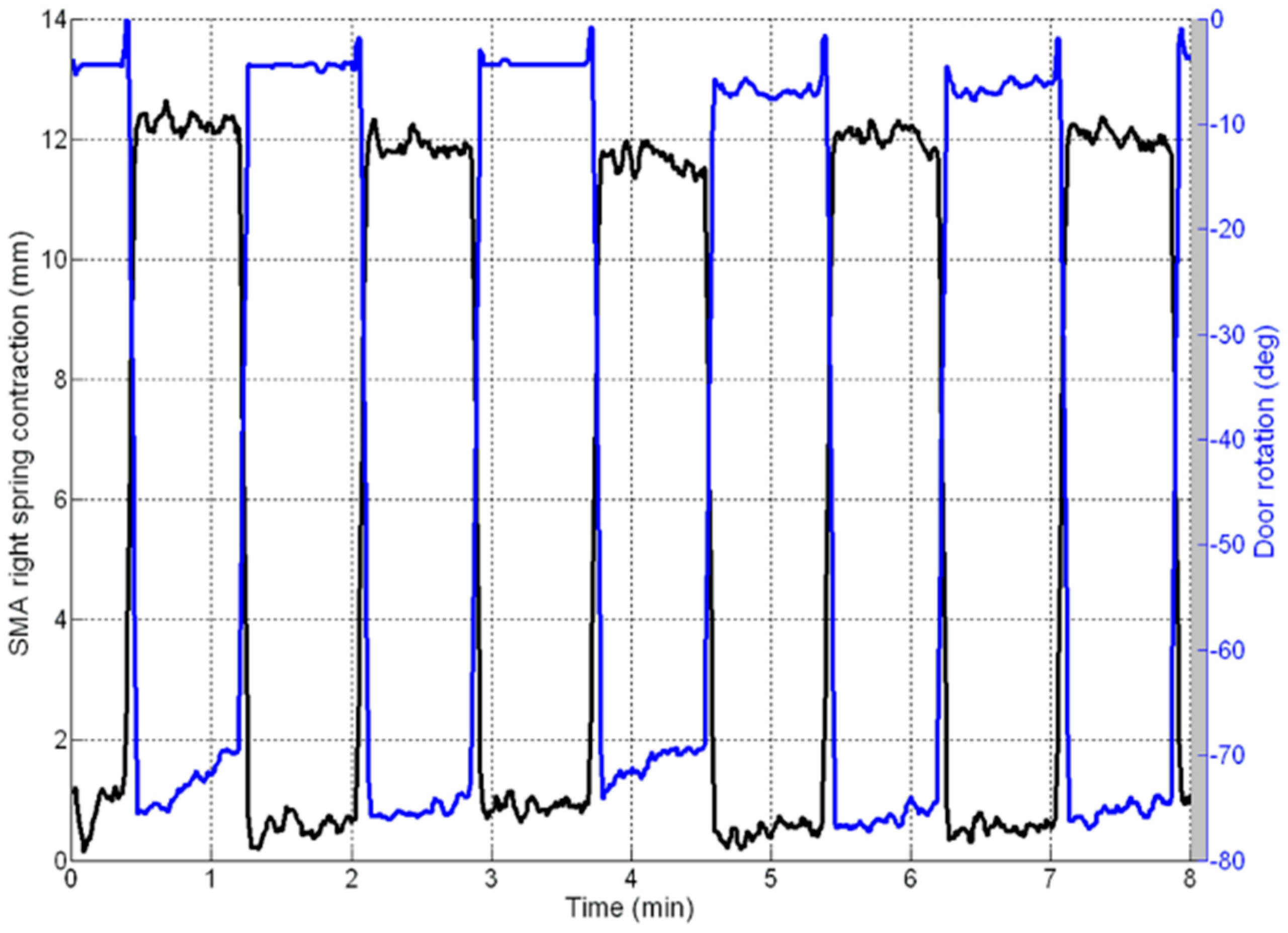
Time diagram,
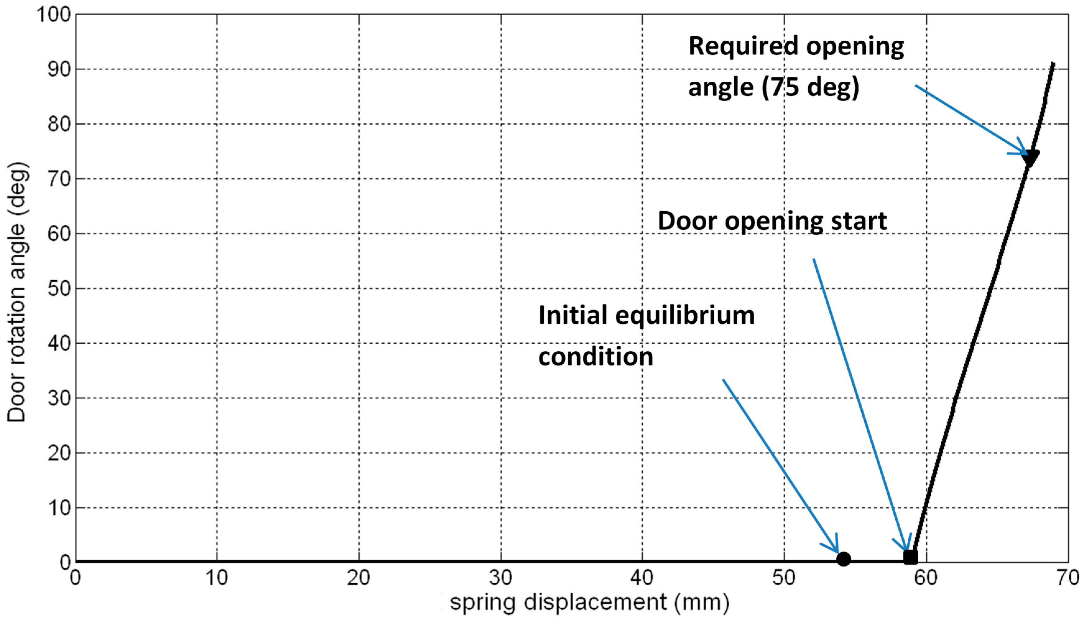
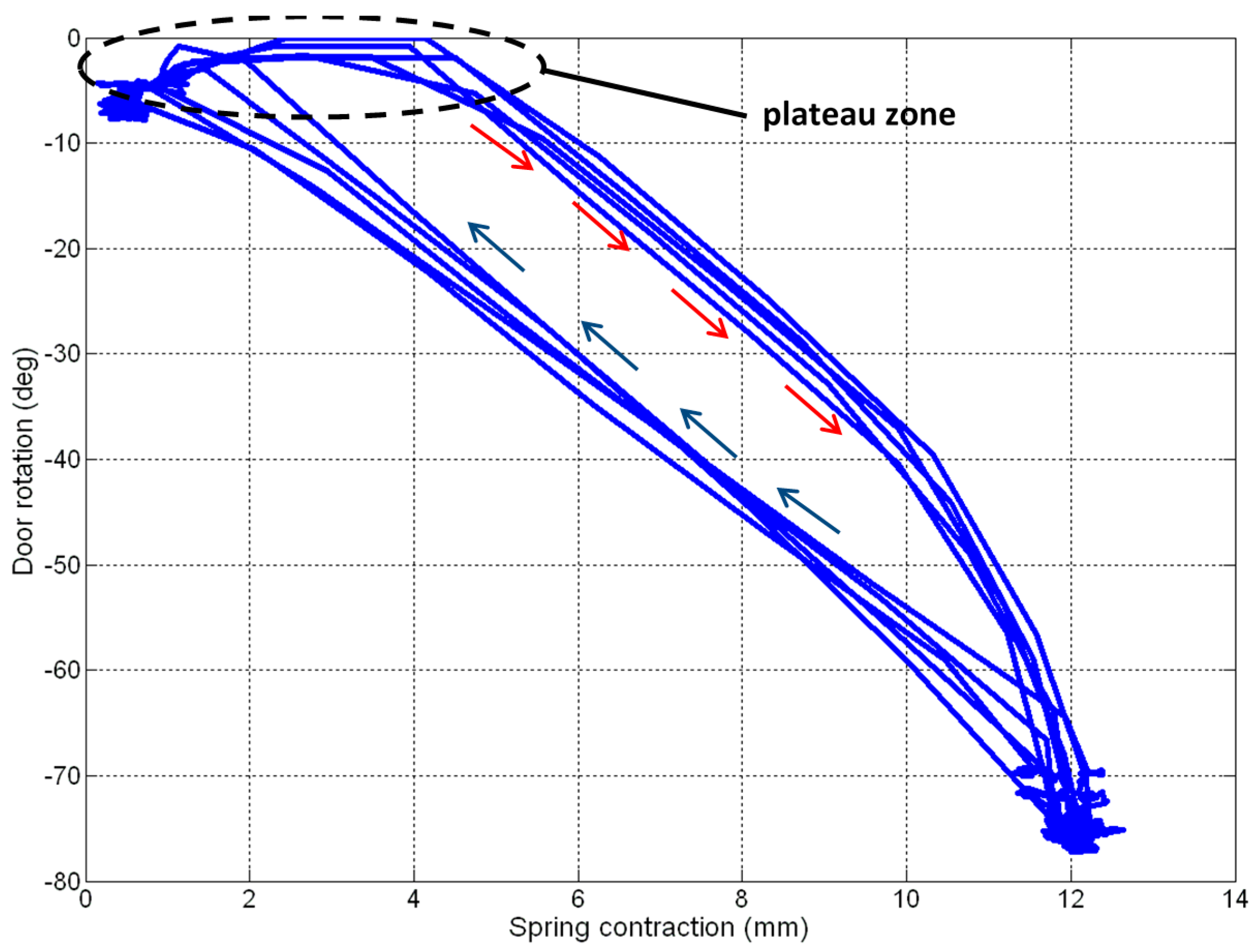
Figure 17, gives a measure of the process repeatability. During the experiment, a max negative angle of 76° was found, in good agreement with the numerical predictions and the specifications. The same cycles are reported in
Figure 18, on the displacement-rotation plane. A plateau ranging from about 0 to 4 mm is evident at the top of the graph, corresponding to the phase when the door remains closed. Both the positioner translation and the total cycle extension are in good agreement with the numerical predictions, previously shown in
Figure 9 (abscissa distance between the “initial equilibrium condition” and the “door opening start” or the “required opening angle of 75°” points, respectively).
A summary and a comparison of the main parameters (numerical and experimental) is provided in
Table 4. From those data, it resulted that a good agreement was found for the kinematic parameters: door opening angle (75° vs. 76°), spring total contraction (12 vs. 10.5 mm), and spring partial contraction until the opening start (4 vs. 3.7 mm). These deviations, due to gaps and free play angles among the system components, can then be easily explained and could be recovered in a controlled realization process.
On the contrary, a larger deviation was observed on the energy estimate per cycle, necessary to drive the SMA springs (11.8 vs. 30.0 J). The numerical prediction was obtained by dividing the mechanical work for stretching the antagonistic element (geometrically represented by the area under the blue line in
Figure 5, between the pre-load and the fully activated conditions) by the characteristic efficiency of 1% [
40]. The experimental value was instead derived by multiplying the fed power by the dispensing time (5 s). Different factors may concur to this deviation: first, the imperfections in this preliminary realization; second, the friction among the different parts; third, the generic dispersions (electrical and mechanical) of the complete system with the surrounding environment. Substantial improvements are then expected when more sophisticated prototypes will be released.


