Comparison of the Average Lift Coefficient ͞C_L and Normalized Lift ͞η_L for Evaluating Hovering and Forward Flapping Flight

Abstract

The capability of flapping wings to generate lift is currently evaluated by using the lift coefficient ${\overline{C}}_L$, a dimensionless number that is derived from the basal equation that calculates the steady-state lift coefficient C_L for fixed wings. In contrast to its simple and direct application to fixed wings, the equation for ${\overline{C}}_L$ requires prior knowledge of the flow field along the wing span, which results in two integrations: along the wing span and over time. This paper proposes an alternate average normalized lift ${\overline{\eta }}_L$ that is easy to apply to hovering and forward flapping flight, does not require prior knowledge of the flow field, does not resort to calculus for its solution, and its lineage is close to the basal equation for steady state C_L. Furthermore, the average normalized lift ${\overline{\eta }}_L$ converges to the legacy C_L as the flapping frequency is reduced to zero (gliding flight). Its ease of use is illustrated by applying the average normalized lift ${\overline{\eta }}_L$ to the hovering and translating flapping flight of bumblebees. This application of the normalized lift is compared to the same application using two widely-accepted legacy average lift coefficients: the first ${\overline{C}}_L$ as defined by Dudley and Ellington, and the second lift coefficient by Weis-Fogh. Furthermore, it is shown that the average normalized lift ${\overline{\eta }}_L$ has a physical meaning: that of the ratio of work exerted by the flapping wings onto the surrounding flow field and the kinetic energy available at the aerodynamic surfaces during the generation of lift. The working equation for the average normalized lift ${\overline{\eta }}_L$ is derived and is presented as a function of Strouhal number, St.

1. Introduction

The lift coefficient C_L is a dimensionless number that evaluates the capability of generating lift by a translating fixed wing subjected to steady state aerodynamics [1] (p. 24):

$$C_L=\frac{L}{\frac{1}{2}·\rho ·{v_{\infty }}^2·s_p}=\frac{L}{q_{\infty }·s_p}$$

(1)

This equation is applied directly to steady-state, fixed wings without further derivation, and the resulting C_L value, which allows for the comparison of dissimilar flyers (i.e., engineering, as well as biological flyers, with fixed wings during gliding) is obtained by normalizing (dividing) lift L by two variables that are widely accepted in the aerodynamic community: the dynamic pressure $q_{\infty }$ (i.e., $\frac{1}{2}·\rho ·{v_{\infty }}^2$) and a reference area, $s_p$, the wing planform area (note the use of lower case symbol $s_p$, to be explained later). This ubiquitous and practical Equation (1) has three peculiarities, the first peculiarity is that it uses the kinetic energy per unit volume of the mass of air, $q_{\infty }$, as it flows over a static airplane, to normalize lift L.

Equation (1) is referred to as a basal equation as the current average lift ${\overline{C}}_L$ that evaluates the ability of generating lift by flapping wings is derived from it. As an example, an average lift coefficient, ${\overline{C}}_{L DE}$, deduced by Dudley and Ellington [2] is shown below:

$$W- L_b={\overline{C}}_{L DE}·\rho ·f·{{\displaystyle \int }}_0^T{{\displaystyle \int }}_0^R{v_r}^2\left(r,t\right)·c\left(t\right)·\cos \mathsf{\Psi }·{\left(1-{\cos }^2\mathsf{\Phi } · {\sin }^2\beta \right)}^{\frac{1}{2}} drdt+ {\overline{C}}_{D DE}· \rho ·f· {{\displaystyle \int }}_0^T{{\displaystyle \int }}_0^R{v_r}^2\left(r,t\right)·c\left(t\right)·\sin \mathsf{\Psi }·{\left(1-{\cos }^2\mathsf{\Phi }·{\sin }^2\beta \right)}^{\frac{1}{2}} drdt$$

(2)

This equation is one of a system of two equations and can be found in [2] (p. 62). This system of equations is applied to hovering and translating flapping flight. A second example, also derived from Equation (1), is the lift average lift coefficient ${\overline{C}}_{L W-F}$, a quick estimate derived by Weis-Fogh [3] (p. 173) that is applied only to hovering flight:

$$L= \frac{1}{2}·\rho ·{\pi }^2·f^2·{\mathsf{\Phi }}^2·{\overline{C}}_{L W-F}·{{\displaystyle \int }}_{r=0}^{r=R}c\left(r\right)·r^{2}dr·{{\displaystyle \int }}_{t=0}^{t=\frac{1}{4}·n·t}{\cos }^2\left(2·\pi ·n·t\right)dt$$

(3)

Solving the above integral results in the following working equation:

$${\overline{C}}_{L W-F}=\frac{4·L}{\rho ·{\pi }^2·f^2·{\mathsf{\Phi }}^2·\sigma ·c·R^3}$$

(4)

Equations (2) and (3) are illustrative of current typical mathematical complications encountered during the derivation of ${\overline{C}}_L$ for flapping wings from the basal equation for C_L.

The complexity of these equations derives from a second peculiarity found in the basal Equation (1): the fact that it only accounts for the translation velocity $v_{\infty }$ but does not account for the average angular velocity $\overline{\omega }$ of flapping wings. The absence of the average angular velocity impedes the direct application of Equation (1) to evaluate the lift-generating capability of flapping wings. In order to apply the equation to flapping wings, the average angular velocity $\overline{\omega }$ must be inserted in Equation (1) by means of an artificial computational construct, the blade element method (BEM) [4] (p. 347), which result in Equations (2) and (3). This construct consists in dividing the flapping wing into a large number of chordwise elements along its span R. Each of these elements of infinitesimally small width are immersed in a unique local flow field that vary along the length of the flapping wing and must be defined a priori by adding the translation velocity vector $v_{\infty }$ (accounted for in Equation (1)) to the local average tangential velocity $v_{tg }$ due to average angular velocity $\overline{\omega }$ of the flapping wing (both velocities $v_{tg }$ and $\overline{\omega }$ are not accounted for in Equation (1)). The resultant of both of these velocities vary along the spanwise length of the wing r as well as with time t (hence, the integrands in Equations (2) and (3) are integrated with respect to dr and dt). In this way, the BEM is the tool that introduces the effect of the average angular velocity $\overline{\omega }$ of flapping wings in Equation (1).

This paper compares the average lift coefficient ${\overline{C}}_L$ with the average normalized lift ${\overline{\eta }}_L$, which has a physical meaning, does not resort to the BEM and is simple to apply to flapping wings during hover and forward flight [5,6].

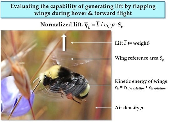
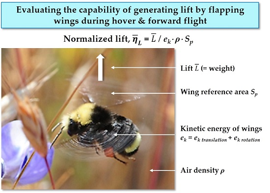
2. The Average Normalized Lift ${\overline{\eta }}_L$

The normalized lift ${\eta }_L$ evaluates the lifting capability of aircraft with a fixed wing during forward (translating) flight and uses the same variables for normalizing the steady state lift L in Equation (1), but reformatted in the following way: the specific kinetic energy available at the wing due to translation, $e_{k trans}$, or $\frac{1}{2}·{v_{\infty }}^2$, the density ρ, and a reference area S_p (note upper case S):

$${\eta }_L=\frac{L}{e_{k trans}·\rho ·S_p}$$

(5)

Note that the density ρ has been “dissociated” from the dynamic pressure $q_{\infty } \left(= \frac{1}{2}·\rho ·{v_{\infty }}^2\right)$ in Equation (1) resulting in the product of the specific kinetic energy, $e_{k trans}$, available at the translating wings, $\frac{1}{2}·{v_{\infty }}^2$, and the density ρ of the surrounding static flow field. This dissociation shifts the legacy reference coordinate system from being affixed to a static lifting surface, say, an aircraft model in a wind tunnel, from which the incoming airflow’s kinetic energy $q_{\infty }$ is being measured, to a new reference coordinate system that is affixed to the static air mass from which the aircraft’s kinetic energy $e_{k trans}$ (or $\frac{1}{2}·{v_{\infty }}^2$) is measured.

Note that Equation (5) has introduced a new definition of the reference area S_p (written in upper case) that differs from the lower case s_p in Equation (1). The original reference area S_p in Equation (1) is found to be its third peculiarity. More on this later.

The term representing the specific kinetic energy (per unit mass) of the flyer, $e_k$ in Equation (5), can be written in a more general format as the total specific kinetic energy available, say, at a lifting rotor that has a translating velocity $v_{\infty }$ and an angular velocity ω. As the presence of these two velocities are accompanied by the possession of corresponding kinetic energies, the total specific kinetic energy $e_k$ can be written as the sum of these two scalar components: the translating kinetic energy $e_{k trans}$ and the rotating kinetic energy $e_{k rot}$:

$$e_k={{\displaystyle \sum }}^{\text{}}{e}_{ki}=e_{k trans}+e_{k rot}= \frac{1}{2}·{v_{\infty }}^2+\frac{1}{2}·\frac{I}{m}·{\omega }^2$$

(6)

The term I/m is the specific moment of inertia (again, per unit mass) of the flapping wing and it accounts for the spanwise mass distribution along its length R. More on this ratio later. To write Equation (5) in a more general format, the kinetic energy term $e_{k trans}$ found in its denominator is replaced by Equation (6). This results in the equation for the normalized lift ${\eta }_L$ that can be applied directly to evaluate the lifting capability of, say, a lift rotor that generates lift L while translating at a velocity $v_{\infty }$ and rotates at an angular velocity ω:

$${\eta }_L=\frac{L}{{{\displaystyle \sum }}^{\text{}}{e}_{ki}·\rho ·S_p}=\frac{L}{\left[\left(\frac{1}{2}· {v_{\infty }}^2 + \frac{1}{2}·\frac{I}{m}·{\omega }^2\right)·\rho ·S_p\right]}$$

(7)

The average normalized lift ${\overline{\eta }}_L$ of flapping wings is obtained by replacing the steady state lift L and angular velocity ω in Equation (7) by the average lift $\overline{L}$ and the average angular velocity $\overline{\omega }$ due to flapping:

$${\overline{\eta }}_L=\frac{\overline{L}}{{{\displaystyle \sum }}^{\text{}}{e}_{ki}·\rho ·S_p}=\frac{\overline{L}}{\left[\left(\frac{1}{2}·{v_{\infty }}^2 + \frac{1}{2}·\frac{I}{m}·{\overline{\omega }}^2\right)·\rho ·S_p\right]}$$

(8)

Throughout this paper, the freestream velocity $v_{\infty }$ and the average angular velocity $\overline{\omega }$ are assumed to remain constant over time. Note that for gliding flight, ω = 0 in Equation (7) and $\overline{\omega }$ = 0 in Equation (8), and as a result, the normalized lift ${\eta }_L$ in Equation (7) and the average normalized lift ${\overline{\eta }}_L$ in Equation (8) equal the steady state lift coefficient C_L in Equation (1). In case of the average lift ${\overline{\eta }}_L$ for gliding or soaring flight, $\overline{\omega }$ = 0, we find that the normalized lift ${\overline{\eta }}_L$ equals the steady state lift coefficient C_L:

$${\overline{\eta }}_L=\frac{\overline{L}}{{{\displaystyle \sum }}^{\text{}}{e}_{ki}·\rho ·S_p}= \frac{\overline{L}}{\frac{1}{2}·{v_{\infty }}^2\rho ·S_p}=C_L$$

(9)

For small values of the average angular velocity $\overline{\omega }$ due to flapping, the quasi-steady state assumption for flapping flight can be invoked and the above steady state equation, Equation (9), can be applied. More on the quasi-steady assumption is given in Section 5.

The quasi-steady assumption tells us that the average normalized lift ${\overline{\eta }}_L$ ≈ lift coefficient C_L with one caveat: the definition of the reference area S_p (symbol in upper case) chosen for both ${\overline{\eta }}_L$ and C_L is the sum of all planform areas of the aerodynamic surfaces that (i) contribute to the net average lift $\overline{L}$ and (ii) are found (close to) perpendicular to the vector lift $\overline{L}$ (the contribution to lift by the fuselage or body is neglected in this paper). This definition of reference area is considered to be physically proper (upper case S_p) whereas the definition of a reference area that does not consider all surfaces contributing to lift (in a positive or negative sense) is considered a physically improper reference area (lower case s_p), as is the case of the legacy reference area s_p of an airplane in Equation (1) (which does not account for tail or canard surfaces, both contributing to lift). In the case of a bumblebee, the physically proper reference area S_p is its total wing area.

The average normalized lift ${\overline{\eta }}_L$ during hover ($v_{\infty }$ = 0 in Equation (8)) is:

$${\overline{\eta }}_L=\frac{\overline{L}}{\frac{1}{2}·\frac{I}{m}·{\overline{\omega }}^2·\rho ·S_p}$$

(10)

Whereas the legacy equations for ${\overline{C}}_L$ in Equations (2) and (4) require prior knowledge of the flow field surrounding a flapping wing (which implies the calculation of the velocity field ahead of each element of the wing along its span r and over time t by resorting to the BEM), Equations (8) (for forward flight) and (10) (for hovering flight) do not require such knowledge, and so, do not resort to the BEM as the average angular velocity $\overline{\omega }$ due to flapping is included in these equations. It is recalled that the sole function of resorting to BEM is to introduce $\overline{\omega }$ of the flapping wings into the basal Equation (1).

With the exception of the ubiquitous usage of the kinetic energy $q_{\infty }$ of a flowing mass of air, the field of aerodynamics does not made extensive use of the concept of energy as do the fields of strength of materials and structure design (i.e., elastic strain energy, Castigliano’s theorem, etc.). Nor has aerodynamics made frequent use of appropriate figures of merit a used in mechanics and thermodynamics. A figure of merit is defined here as a dimensionless number that (i) possesses a physical meaning, that of a ratio of work w and kinetic energy e_k; (ii) uses only physically proper parameters for normalizing (dividing) the average lift $\overline{L}$ (or average drag $\overline{D}$ and thrust $\overline{T}$, forces not covered in this paper), that is, parameters that have a dominant effect in the generation of lift $\overline{L}$; (iii) is associated with a maximum value ${\overline{\eta }}_{L \text{max}}$ which is usually empirical in nature, and (arguably) close to 1; and (iv) can be read on a stand-alone basis as a “high” or a “low” value.

The average normalized lift ${\overline{\eta }}_L$ is a figure of merit like the efficiency η used in mechanics and thermodynamics, and has the same physical significance: the ratio of work and energy.

The physical meaning of the average normalized lift ${\overline{\eta }}_L$ is the ratio of the work w (=$\overline{L}/\rho ·S_p$) exerted by the surface S_p and the kinetic energy e_k available at this reference surface S_p during the generation of the average net lift $\overline{L}$ [5]. This ratio w/e_k is made apparent by rewriting Equation (8) as:

$${\overline{\eta }}_L=\frac{\frac{\overline{L}}{\rho ·S_p}}{\frac{1}{2}·{v_{\infty }}^2 + \frac{1}{2}·\frac{I}{m}·{\overline{\omega }}^2}=\frac{w}{e_k}$$

(11)

Note that when the wing loading, $\overline{L}/S_p$, found in the numerator of Equation (11), is divided by the density ρ, it results in the specific work w exerted by the flapping wings.

Equation (11) does not imply that the average lift $\overline{L}$ generated by flapping is sensitive to the specific moment of inertia I/m of the flapping wings, but the average normalized lift ${\overline{\eta }}_L$ is. The above equation format (i.e.; w/e_k) allows for a novel physical interpretation of the normalized lift, an interpretation that is shared with all physically proper lift coefficients C_L, as applied, say, to a fixed-winged airplane (ω = 0 in Equation (11)) as it accelerates gradually during straight and level flight as it generates a constant amount of lift L (equal to its weight W) while gradually reducing its angle of attack. In this scenario, the work exerted by the fixed wing, L/ρ·S_p, remains constant (L = W = constant) whereas the kinetic energy $\frac{1}{2}·{v_{\infty }}^2$ available at the wing gradually increases. Its normalized lift ${\eta }_L$ (or lift coefficient C_L) measures the amount of work w done “per kinetic energy available” e_k that is found to reduce gradually as evidenced by the gradual reduction of the angle of attack. In other words, L/ρ·S_p remains constant in the numerator of Equation (11), whereas its denominator gradually increases, resulting in a decrease of the normalized lift ${\eta }_L$ (or lift coefficient C_L). This physical concept is applicable to the lift coefficient C_L as long as it is calculated by normalizing lift L by physically proper parameters only. The use of one or more physically improper parameters for calculating C_L will render it also physically improper and unfit for use for comparing different lifting surfaces (say, between flapping wings and rotating cylinders in Magnus effect). At this point, and possibly addressing the possible question raised by the reader on the purpose or validity of comparing such differing lifting systems, it is argued that the usefulness of a figure of merit may be seen to increase if these comparisons, however unlikely, are allowed as meaningful (in the same way the efficiency η of, say, the Otto cycle and a jet engine’s Brayton cycle can be compared in thermodynamics). The use of physically improper parameter(s) will result in physically improper legacy coefficients C_L and C_Do that do not allow for such meaningful comparisons, as is the case when comparing the lift coefficient C_L of different aircraft configurations (e.g.; flying wing against tail-configured aircraft) or when comparing the parasite drag coefficient C_Do of airplanes of different wing areas (e.g.; F-104 Starfighter against B-58 Hustler). When using these legacy coefficients, meaningful comparisons can still be made by limiting the comparison of C_L to airplanes of same configuration (flying wing against flying wing), or comparing the C_Do of airplanes with same physically improper reference area s_p [5].

Enter the third peculiarity of Equation (1): as mentioned above, a valid side-by-side comparison of the normalized lift ${\eta }_L$ of steady state lift systems (i.e., fixed-wing aircraft) as well as the average normalized lift ${\overline{\eta }}_L$ for time-dependent lift systems (i.e., bumblebees) requires a consistent, physically proper reference area: the reference surface S_p (upper case S) in Equation (5) (and onwards) is the total planform area found (close to) perpendicular and contributing to the net average lift $\overline{L}$. As discussed above, an expected application of a dimensionless coefficient, be it the lift coefficient C_L, the normalized lift ${\eta }_L$ or its average value ${\overline{\eta }}_L$ is the comparison of the ability of generating lift L by various types of lift systems, be these designed by engineers (i.e., tail or canard-configured airplanes, lift rotors, ornithopters) or researched by biomechanicists (i.e., flapping wings of bumblebees). As mentioned, the possibility of a side-by-side comparison of these differing systems has a valuable cross-pollination potential that unfortunately is not currently possible as the definition of a reference area selected for normalizing steady-state lift L of aircraft (with a reference area represented by a lower case s_p in Equation (1)) is not consistent with the definition of a reference area used for normalizing the time-dependent lift $\overline{L}$ in biological flight (with a reference area represented by an upper case S_p in Equation (5) and onwards). The average lift coefficient ${\overline{C}}_L$ of a bumblebee is obtained by normalizing its lift $\overline{L}$ by all the aerodynamic surfaces contributing to its generation, an all-inclusive definition made explicit by the use of the upper case symbol, S_p, as shown in Equation (5). In contrast, and here is the third peculiarity of C_L in Equation (1), the reference area used for a tail or canard-configured airplane considers only the main wing planform s_p. This definition of the legacy s_p, suggested by Munk in 1923 [6], excludes the tail surface and so, neglects its contribution to the net lift L (usually a negative one due to stability purposes) as well as the canard surface (and so, neglects its contribution to the net lift L, always a positive one). This non-inclusive definitions of reference area is a third peculiarity of Equation (1) that results in an physically improper parameter, and is made explicit in this paper by choosing for a lower case symbol, s_p, as shown in Equation (1).

The inconsistency in the definition of reference areas results in, say, the bumblebee having a relatively lower wing loading $\overline{L}/S_p$, whereas the tail and canard-configured airplanes will have a higher wing loading L/s_p (as tail and canard areas are not accounted for). This results in an “inflated” wing loading (as s_p < S_p, so L/s_p > $\overline{L}/S_p$) for the tail and canard-configured airplanes when compared to a bumblebee. This larger wing loading, when divided by the density ρ (as per Equation (11)) results, again, in an “inflated” work w exerted by the tail and canard-configured airplanes, which in turn results in an inflated ${\overline{\eta }}_L$ (and ${\overline{\eta }}_{L \text{max}}$) when compared to a bumblebee. This inflated value can be mistakenly reported as a result of a Reynolds number effect but is, instead, due to an inconsistency in the definition of reference areas. That an increase in the Reynolds number has an effect of an increase in C_{L max} is not in question: what is highlighted here is a significant contribution towards an increase in the lift coefficient C_L (and C_{L max}) that is a result of a more mundane problem: the neglect of the tail and canard areas. If comparisons between biological flyers and aircraft are necessary, the reader is encouraged to compare their legacy C_L (and C_{L max}) values using flying wings instead of tail and canard-configured airplanes. In other words: the comparison of the capability of generating lift by tail and canard-configured airplanes on one side and bumblebees on the other may be flawed due to the use of inconsistent definition of their reference areas that, by neglecting a large percentage of their lifting areas that contribute to net lift (≈ tail and canard are typically 20% of the total lifting planform) invalidates a meaningful comparison between lift coefficients, as results show an overestimate of the lift capability of tail and canard-configured by, typically, 20%. Although not related to flapping flight, the above-described situation also arises when comparing the (inevitably lower) C_{L max} of a flying wing with the C_{L max} of a tail or canard-configured aircraft. The normalized lift ${\eta }_L$ is a figure of merit that is not configuration-dependent and allows for the meaningful comparison of a large variety of lifting systems due to its use of a consistent, physically proper definition of reference area S_p [5].

Next, we evaluate two physically proper parameters found in Equation (11): the average angular velocity $\overline{\omega }$ and the specific moment of inertia I/m. From these parameters, other physically proper parameters will be derived, and their inclusions in Equation (11) will make this equation more practical.

The average angular velocity $\overline{\omega }$ of flapping wings in Equation (11) equals 2·f·Φ where f is the flapping frequency in cycles per second (a cycle is a downstroke followed by an upstroke) and Φ is the stroke angle (a stroke is the wing’s upstroke or downstroke).

The specific moment of inertia I/m in Equation (11) is the specific moment of inertia of a single flapping wing, a term that is not related to aerodynamics but to its spanwise (not chordwise) mass distribution. The specific moment of inertia I/m of a wing is related to the second moment of inertia, but from a “kinetic energy-during-flapping” standpoint that occupies us here, the chordwise placement of the wing’s center of gravity, CG, is neglected. This is so as is the wing pronation/supination involves a negligible amount of kinetic energy as the wing rotates about the wing’s long axis during each flapping cycle. So, the “second moment” scenario is now a “first moment” one, were the two-dimensional wing is substituted by a one-dimensional rod of constant density distribution along its length, a valid substitution as long as the wing’s spanwise CG location coincides with the rod’s CG (as the rod of length R has a constant density along its length R, its center of gravity is placed at R/2). From an inertial standpoint and from a “per unit basis” (and understanding that aerodynamics does not play a role in I/m) the flapping wing will have the same inertial property (i.e., I/m) as the rod, as long as both (i) share the same kinetic characteristics (wing pronation and supination during flapping are not considered) and (ii) the CG of the wing and rod are placed at the same spanwise distance dCG from the axis of rotation. Whereas the length R of the wing and the rod may be different, the distance of their CG to the axis of rotation dCG must be the same for this substitution to be valid (i.e., same dCG). So, if the CG of the wing is not known, the term I/m is obtained by replacing the wing by a cylindrical rod of the same length R as the wing’s span. It is not necessary to know the mass m of the wing as Equation (11) contains specific kinetic energy terms e_k, that is, energies per unit mass.

There are two cases to contemplate: as mentioned above, if the CG of the wing is not known, it can be assumed to be at half the wing’s length, R/2, and so, its specific moment of inertia I/m can be substituted by the moment of inertia per unit mass of a rod as it rotates about its end and equal to ⅓·R², a value found in [7] (p. 251, Figure 9f). The 1/3 value is what Weis-Fogh calls the shape factor for the second moment of the area, σ [3] (p. 173, Table 1, first row). The second case is when the center of gravity of the wing can be calculated and is not found to be at (or close to) R/2 on the wing but at a distance, say, dCG, from the axis of rotation. In this case, the rod substituting the wing will be of length 2·dCG, and its specific moment of inertia I/m of the wing becomes ⅓·(2·dCG)².

If the assumption of the placement of the center of gravity of the wing at R/2 is acceptable, then I/m in Equation (11) can be replaced with ⅓·R², and $\overline{\omega }$ is replaced by 2·f·Φ, and the fraction ½ is made a common factor and placed outside of the parentheses. With these changes made in the denominator of Equation (11), we define the total wing velocity V_w of a flapping wing as:

$$V_w={\left[{v_{\infty }}^2+\left(\frac{I}{m}\right)·{\overline{\omega }}^2\right]}^{\frac{1}{2}}={\left[{v_{\infty }}^2+\left(\frac{1}{3}·R^2\right)·{\left(2·f·\mathsf{\Phi }\right)}^2\right]}^{\frac{1}{2}}= {\left[{v_{\infty }}^2+ \frac{1}{3}·{\left(2·f·\mathsf{\Phi }·R\right)}^2\right]}^{\frac{1}{2}}$$

(12)

The product $\mathsf{\Phi }·R$ equals the peak-to-peak amplitude A travelled by the wing tip along a upstroke (or a downstroke) and if multiplied by the frequency 2·f, it results in the average tangential velocity v_tt of the wing tip (subscript tt stands for tip, tangential) during a stroke. Replacing in Equation (12), the total velocity V_w is:

$$V_w={\left[{v_{\infty }}^2+\frac{1}{3}·{\left(2·f·\mathrm{A}\right)}^2\right]}^{\frac{1}{2}}= {\left[{v_{\infty }}^2+ \frac{1}{3}·{v_{tt}}^2\right]}^{\frac{1}{2}}$$

(13)

For a non-zero translating flight velocity, $v_{\infty }$ ≠ 0 in Equation (13), the translation velocity v_∞ is made a common factor and, when taken out of the parentheses, the above expression is written as a function of the velocity ratio $v_{tt}/v_{\infty }$ that equals the Strouhal number, St [8]:

$$V_w=v_{\infty }·{\left[1+\frac{1}{3}·{\left(\frac{v_{tt}}{v_{\infty }}\right)}^2\right]}^{\frac{1}{2}}= v_{\infty }·{\left(1+\frac{1}{3}·S{t}^2\right)}^{\frac{1}{2}}$$

(14)

This definition of the total wing velocity V_w is based on kinetic energy considerations and varies from Lentink and Dickinson’s definition of the characteristic speed U, which derives from the kinematics of the flapping wing [9] (p. 2695).

In the same vane, the total dynamic pressure Q is defined as a function of total velocity V_w and the Strouhal number St:

$$Q=\frac{1}{2}·\rho ·{V_w}^2=\frac{1}{2}·\rho ·{v_{\infty }}^2·\left(1+\frac{1}{3}·S{t}^2\right)= q_{\infty }·\left(1+\frac{1}{3}·S{t}^2\right)$$

(15)

The total dynamic pressure Q results from the addition of the dynamic pressure due to the wing translation, $q_{\infty }$, and the dynamic pressure due to flapping, and should not be confused with the total pressure p₀, the sum of static and dynamic pressure. Note that for the translating flight of fixed wings (i.e., gliding flight), the flapping frequency f is 0, and so, the Strouhal number St is zero, and the total velocity V_w is then reduced to the freestream velocity at infinity, V_w = $v_{\infty }$, in Equation (14). Furthermore, the total dynamic pressure Q is reduced to the dynamic pressure $q_{\infty }$ in Equation (15).

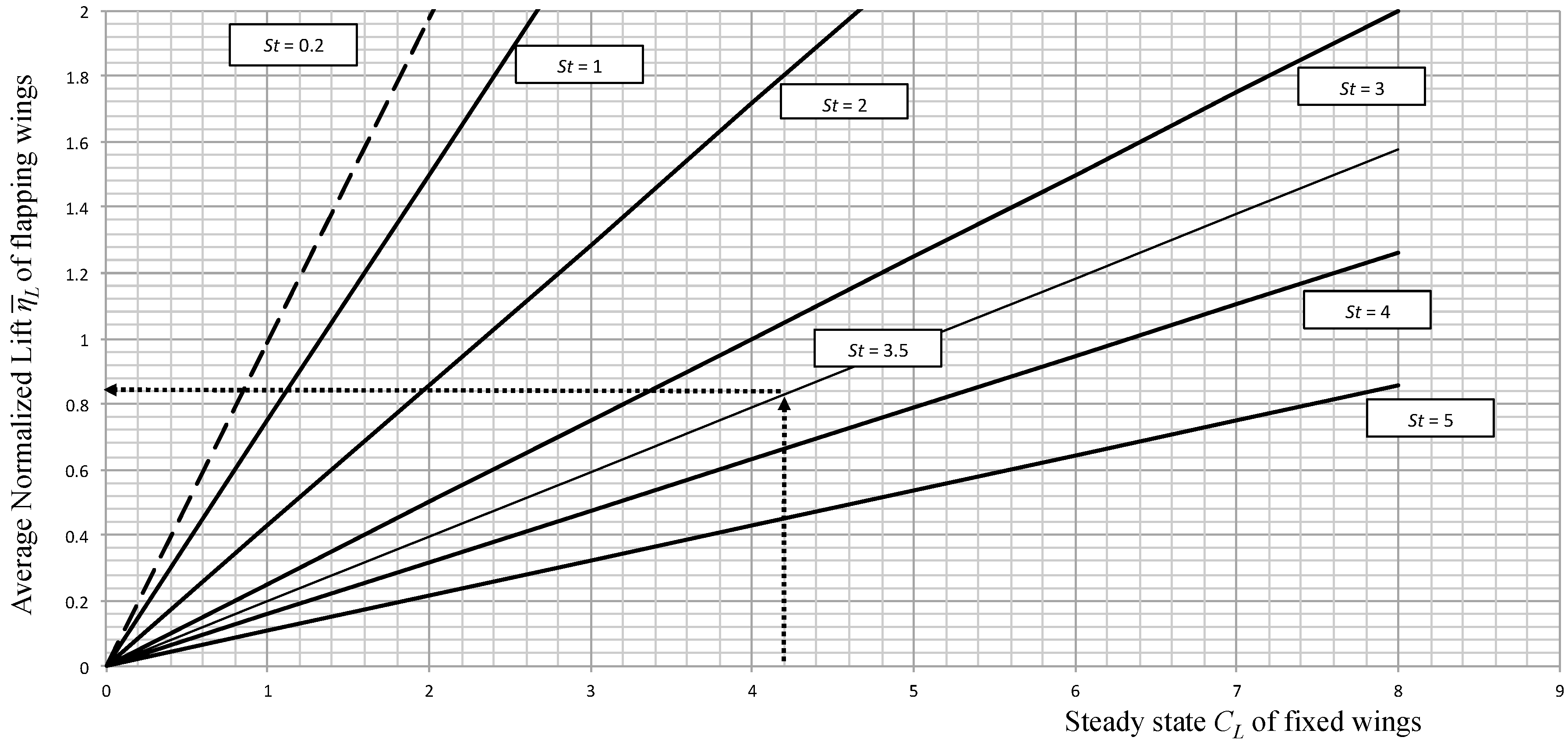
The average normalized lift ${\overline{\eta }}_L$ of flapping wings is next written as a function of Strouhal number:

$${\overline{\eta }}_L=\frac{\overline{L}}{\frac{1}{2}·\rho ·{v_{\infty }}^2·\left(1+\frac{1}{3}·S{t}^2\right)·S_p}$$

(16)

The relationship between the steady state lift coefficient C_L and the time-dependent average normalized lift ${\overline{\eta }}_L$ is evaluated by the ratio $C_L/{\overline{\eta }}_L$, or the ratio Equation (1)/Equation (16):

$$\frac{C_L}{{\overline{\eta }}_L}=1+ \frac{1}{3}·S{t}^2$$

(17)

As the flapping frequency f tends to 0 for a given forward velocity $v_{\infty }$, the Strouhal number St tends to 0 and ${\overline{\eta }}_L$ tends to C_L (f→0, then St→0 and $C_L/{\overline{\eta }}_L$→1). Equation (17) can be used to advantage to calculate the average normalized lift ${\overline{\eta }}_L$ in two steps: the first step calculates the coefficient C_L for the steady state flight (by assuming extended wings and simply not considering its flapping kinematics) using Equation (1). The second step “corrects” C_L for the time-dependent effects of flapping by dividing the steady state C_L by 1 + ⅓·St². The lift coefficient C_L in Equation (17) during flapping flight can be interpreted as the hypothetical steady-state lift coefficient C_L required from the extended, non-flapping wings as they generate an (unrealistic) lift L equal to the weight of the flyer as it translates at the same forward speed $v_{\infty }$ as the actual flapping flyer. This steady state C_L is unrealistic as the wings will stall at a much lower value. Correcting this steady-state fictitious C_L value by dividing it (1 + ⅓·St²) results in the average normalized lift ${\overline{\eta }}_L$ of the flapping wings of the flyer. A quasi-steady analysis of flapping flight can be contemplated when the values of the steady state lift coefficient C_L and the corresponding average normalized lift ${\overline{\eta }}_L$ are close (i.e.; C_L ≈${\overline{\eta }}_L$). More on this subject in Section 5.

The total velocity V_w defined in Equation (14) can be used to advantage to characterize the Reynolds number of flapping wings of characteristic chord c, surrounded by the air of kinematic viscosity, υ:

$$Re= \frac{V_w·c}{\upsilon }=\left(\frac{v_{\infty }·c}{\upsilon }\right)·{\left(1+\frac{1}{3}·S{t}^2\right)}^{\frac{1}{2}}= R{e}_{ss}·{\left(1+\frac{1}{3}·S{t}^2\right)}^{\frac{1}{2}}$$

(18)

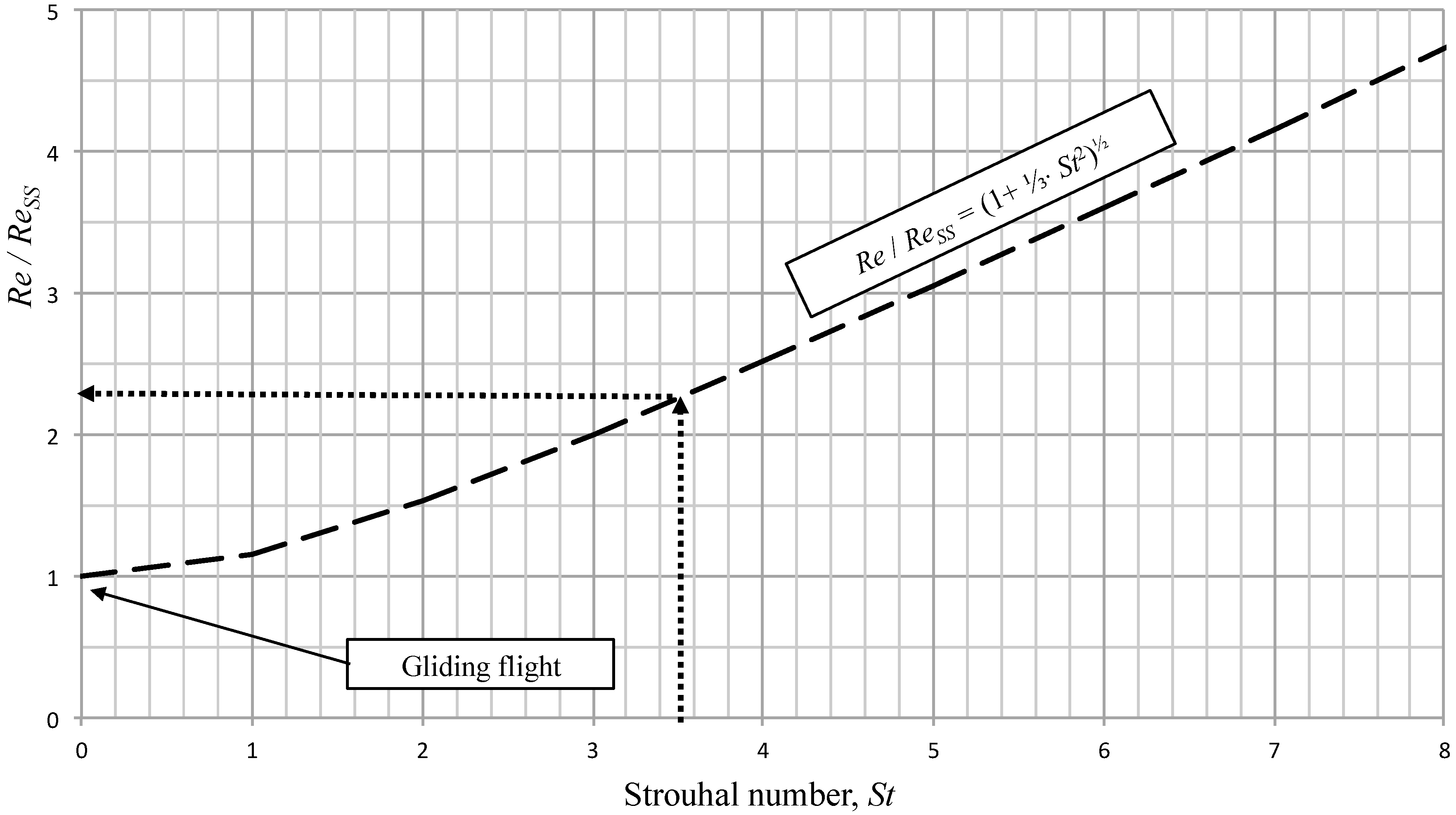
The Reynolds number Re due to flapping can be calculated in two steps: the first step calculates the steady state Reynolds number Re_ss (the subscript ss stands for steady state) contained in the leftmost parentheses, and the second step corrects Re_ss for flapping effects by multiplying it by (1 + ⅓·St²)^½. A closely-related approach to evaluating the Reynolds number of flapping wings has been suggested by Lentink and Dickinson [9] (p. 2696).

The average normalized lift ${\overline{\eta }}_L$ can be written in a familiar format, as a function of the total velocity V_w or the total dynamic pressure, Q,

$${\overline{\eta }}_L= \frac{\overline{L}}{\frac{1}{2}·\rho ·{V_w}^2·S_p}=\frac{\overline{L}}{Q·S_p}$$

(19)

The following

Table 1. Time-dependent variables obtained from steady state variables.

Time-Dependent Variable	Time-Dependent Variables as a Function of Steady State Parameters	Equation No.
Total velocity, Vw	Vw = v∞·(1 + ⅓·St2)½	14
Total dynamic pressure, Q	Q = q∞·(1 + ⅓·St2)	15
Average normalized Lift, ${\overline{\eta }}_L$	${\overline{\eta }}_L$ = CL·(1 + ⅓·St2)−1	17
Reynolds number, Re	Re = Ress·(1 + ⅓·St2)½	18

shows how the time-dependent variables V_w, Q, ${\overline{\eta }}_L$ and Re can be calculated by “correcting” the corresponding steady-state parameters $v_{\infty }$, $q_{\infty }$, C_L and Re_ss by the term (1 + ⅓·St²):

For illustration purposes,

Table 2. Strouhal number effect on total dynamic pressure Q and Reynolds number Re of flapping wings.

St	1 + ⅓·St2	Q/q∞	Re/Ress
0	1.00	1.00	1.00
1	1.33	1.33	1.15
2	2.33	2.33	1.53
3	4.00	4.00	2.00
4	6.33	6.33	2.52
5	9.33	9.33	3.06
6	13.00	13.00	3.61
7	17.33	17.33	4.16
8	22.33	22.33	4.73
9	28.00	28.00	5.29
10	34.33	34.33	5.86

shows how the correction factor (1 + ⅓·St²), the ratio of total dynamic pressure and dynamic pressure, Q/q_∞, and the ratio of the Reynolds number of a flapping wing and the corresponding steady state Reynolds number of the same wing, Re/Re_ss, vary with Strouhal number, St:

A desirable feature of the average normalized lift ${\overline{\eta }}_L$ is its association with an empirical maximum value, ${\overline{\eta }}_{L \text{max}}$, that makes it possible to read it on a stand-alone basis, as a “high” or “low” value, relative to ${\overline{\eta }}_{L \text{max}}$. In a similar way, the lift coefficient $C_L$ of a fixed lifting surface can also be read on a stand-alone basis (which does not necessarily imply it is a physically proper figure of merit). This feature should not be taken for granted as is illustrated by the ubiquitous drag coefficient $C_D$ of an airplane of, say, 0.0345 or 345 counts (calculated using the customary wing planform as a reference area). This value cannot be read on a stand-alone basis as this value is not associated to a common maximum value C_{D max}, and so, cannot be read as a “high” or low” value.

3. Evaluation of ${\overline{C}}_L$ and ${\overline{\eta }}_L$ of Hovering Bumblebees

This section compares the application of the normalized lift ${\overline{\eta }}_L$ against the two legacy and well known legacy coefficients ${\overline{C}}_L$ derived from the basal $C_L$ equation using the BEM. One lift equation is the one derived by Dudley and Ellington (subscript DE), Equation (2), and the second equation is derived by Weis-Fogh (subscript W–F), shown in Equations (3) and (4). In this section, these dimensionless numbers, ${\overline{\eta }}_L$, ${\overline{C}}_{L DE}$, and ${\overline{C}}_{L W-F}$ are calculated for three bumblebees during hovering flight. Data on weight W, reference area S_p and wing root-to-tip length R for the three bumblebees BB01, BB02, and BB03 are presented in

Table 3. Weight and wing geometric parameters of the three bumblebees.

ID	W (N)	Sp (m2)	R (m)
BB01	0.00172	0.00011	0.0132
BB02	0.0018	0.0001	0.0137
BB03	0.00583	0.0137	0.0154

and were obtained from Dudley and Ellington [10] (p. 32, Table 1):

Furthermore, kinematic data of these bumblebees are also given by Dudley and Ellington and are presented in

Table 4. Kinematic data of the flapping wings of the three bumblebees during hover.

ID	f (Hz)	Φ (rad)	$\overline{\omega }$ (1/s)
BB01	155	2.02	627.57
BB02	147	1.82	533.61
BB03	166	2.27	753.23

[2] (Figures 8–10, Part A, pp. 38–40). During hover, the air density ρ is 1.23 kg/m³ at sea level, and the kinematic viscosity υ is assumed to be 1.46 × 10⁻⁵ m²/s, corresponding to the according to the standard atmosphere [11].

The average lift coefficient ${\overline{C}}_{L DE}$ is calculated by Dudley and Ellington using Equation (2) and read from a graph in [2] (p. 72, Figure 10), and the quick estimates ${\overline{C}}_{L W-F}$ by Weis-Fogh’s using Equation (3), and the average normalized lift ${\overline{\eta }}_L$ is calculated using Equation (10). Results are presented in

Table 5. Averages of the two legacy average lift coefficients ${\overline{C}}_L$ and the average normalized lift ${\overline{\eta }}_L$ for the three bumblebees during hover. Note lower average value of 1.29 for average normalized lift ${\overline{\eta }}_L$.

ID	${\overline{C}}_{L DE}$	${\overline{C}}_{L W-F}$	${\overline{\eta }}_L$
BB01	1.2	1.87	1.15
BB02	2.1	2.35	1.45
BB03	2.65	2.09	1.29
Average	1.98	2.01	1.29

below.

.

The average normalized lift ${\overline{\eta }}_L$ has the lowest average.

4. Evaluating ${\overline{C}}_L$ and ${\overline{\eta }}_L$ of Forward Flying Bumblebees

This section compares the average lift coefficient ${\overline{C}}_{L DE}$ by Dudley and Ellington with the average normalized lift ${\overline{\eta }}_L$. Weis-Fogh’s lift coefficient as per Equation (4) is not included in this study as his equation is only fit for evaluating hovering flight. The forward velocity $v_{\infty }$, frequency f, and flapping stroke angle Φ, shown in the first three columns in

Table 6. Kinematic data of flapping wings, flight data, Dudley and Ellington’s average lift coefficient ${\overline{C}}_{L DE}$, average normalized lift ${\overline{\eta }}_L$ , and the ratio of flapping Re to steady-state Re_ss.

ID	$v_{\infty }$ (m/s)	f (Hz)	Φ (rad)	$\overline{\omega }$ (1/s)	vtt (m/s)	St	${\overline{\eta }}_L$	${\overline{C}}_{L DE}$	(1 + ⅓·St2)½	Re/Ress
BB01	0	155	2.02	627.57	–	–	1.15	1.2	–	–
	1	145	1.95	566.84	7.48	7.48	1.34	1.72	19.66	4.43
	2.5	152	2.18	663.18	8.75	3.50	0.83	1.28	5.09	2.26
	4.5	144	1.80	517.70	6.83	1.52	0.74	1.15	1.77	1.33
BB02	0	147	1.82	533.61	–	–	1.45	2.1	–	–
	1	132	1.73	456.13	6.25	6.25	1.84	2.18	14.02	3.74
	2.5	132	2.01	529.84	7.26	2.90	1.09	1.8	3.81	1.95
	4.5	143	1.66	474.17	6.50	1.44	0.75	1.05	1.69	1.30
BB03	0	166	2.27	753.23	–	–	1.29	2.65	–	–
	1	157	2.22	695.95	10.72	10.72	1.47	3.25	39.29	6.27
	2.5	141	1.68	472.46	7.28	2.91	2.42	2.1	3.82	1.96

represent data of the three bumblebees at the different forward velocities of 1, 2.5, and 4.5 m/s [2] (Figures 8–10, Part A, pp. 38–40). The next three columns show the calculated mean flapping angular speed $\left(\overline{\omega }=f·\mathsf{\Phi }\right)$, the tangential tip velocity $\left(v_{tt}=\overline{\omega }·R\right)$, and Strouhal number $\left(St=\frac{2·f·\mathsf{\Phi }·R}{v_{\infty }}\right)$. The next two columns show the average normalized lift, ${\overline{\eta }}_L$, Equation (16) and the average lift coefficient ${\overline{C}}_{L DE}$ by Dudley and Ellington using Equation (2). The final column shows the ratio of the actual Reynolds number of the flapping wing and the Reynolds number Re_ss corresponding to the steady state for the same wing as it flies at the same translating velocity $v_{\infty }$ as the flapping wing).

These tabular values in Table 6 values are represented graphically in Figure 1, showing the average lift coefficients ${\overline{C}}_{L DE}$ (dashed line data, copied from [2] (p. 72, Figure 10)) and average normalized lift values ${\overline{\eta }}_L$ (continuous lines) for hover ($v_{\infty }$ = 0, along the ordinate axis) and forward flight, as a function of forward speed $v_{\infty }$.

Table 7. The Dudley and Ellington’s average lift coefficient ${\overline{C}}_{L DE}$, and the average normalized lift ${\overline{\eta }}_L$, and corresponding averages for forward flight.

ID	${\overline{C}}_{L DE}$	${\overline{\eta }}_L$	${\overline{C}}_{L DE}$	${\overline{\eta }}_L$	${\overline{C}}_{L DE}$	${\overline{\eta }}_L$
	1 m/s		2.5 m/s		4.5 m/s
BB01	1.72	1.34	1.28	0.83	1.15	0.74
BB02	2.18	1.84	1.8	1.09	1.05	0.75
BB03	3.25	1.47	2.1	–	–	–
Average	2.38	1.55	1.73	1.89	1.89	1.89

shows results for ${\overline{C}}_{L DE}$ and ${\overline{\eta }}_L$.

Dudley and Ellington have stated that no good quality for the average lift coefficient ${\overline{C}}_L$ was obtained for bumblebee queen BB03 at $v_{\infty }$ of 4.5 m/s [10] (p. 35). According to their data though, no abnormality was found in the average lift coefficient of BB03 at the prior speed of 2.5 m/s, which measured a ${\overline{C}}_{L DE}$ of 2.1, as shown in Figure 1. At this speed, the average normalized lift ${\overline{\eta }}_L$ of BB03 is anomalously high, 2.42, as shown as a grey symbol “$●$” in Figure 1.

Based on this data, the normalized lift ${\overline{\eta }}_L$ may be better suited for diagnosis and detection of anomalous flight data.

5. Evaluating the Aerodynamics of Bumblebee BB01

The average normalized lift ${\overline{\eta }}_L$ of, say, bumblebee BB01 as it flies at a forward speed of 2.5 m/s has been found to be 0.83, as shown in the third row, seventh column in Table 6. This value can be easily computed with the aforementioned two-step approach and implied in Equation (17), repeated below for convenience,

$${\overline{\eta }}_L=\frac{C_L}{\left(1+ \frac{1}{3}·S{t}^2\right)}$$

(20)

When using this approach, both the normalized lift ${\overline{\eta }}_L$ and the steady state lift coefficient C_L are calculated using the same physically proper reference area S_p, as defined in Section 2 (i.e.; the total wing area of the bumblebee). The first step calculates the steady state (non-flapping) lift coefficient C_L of the bumblebee using Equation (1), using the following information: its weight W of 0.001715 N, its reference area S_p of 0.000106 m², the density at sea level of 1.23 kg/m³, and a forward velocity $v_{\infty }$ of 2.5 m/s. The resulting steady state lift coefficient C_L equals 4.2, an obviously unrealistic value that is much higher than the maximum value C_{L max} that can be possibly reached during steady state at these low (or any) Reynolds numbers (the steady state value for C_{L max} at this Reynolds numbers is likely < 1). The second step modifies this steady state lift coefficient C_L by dividing it by the “correction factor” (1 + ⅓·St²) to account for the effects of time-dependent flow. This correction factor is 5.08, where the Strouhal number St is 3.5 $\left(St=\frac{2·f·\mathsf{\Phi }·R}{v_{\infty }}=\frac{2·152·2.18·0.0132}{2.5}\right)$. The resulting average normalized lift ${\overline{\eta }}_L$ is 0.83 (= 4.2/5.08).

This second step can also be obtained graphically using Figure 2 by entering the steady state C_L of 4.2 and intersecting the isoline corresponding to a constant Strouhal number St of 3.5, and reading the resulting average normalized lift of ${\overline{\eta }}_L$ on the vertical axis: 0.83.

Figure 2 shows a region delimited by the (vertical) ordinate axis and the isoline for St = 0.2 (dashed line). This area represents the quasi-steady region where the average normalized lift ${\overline{\eta }}_L$ of flapping flight using Equation (16) is close to its steady-state C_L calculated using Equation (1). In other words, for flight conditions where the Strouhal number St is equal or less than 0.2, then ${\overline{\eta }}_L$ ≈ C_L and so, it can be estimated by C_L, and the actual average normalized lift ${\overline{\eta }}_L$ is smaller than C_L by 1.33%. If St = 0.3, ${\overline{\eta }}_L$ is smaller than C_L by 2.91% and for St = 1, ${\overline{\eta }}_L$ is smaller than C_L by 33%.

The ratio of the Reynolds number, Re, of a flapping wing and the Reynolds number Re_ss for the corresponding steady state, non-flapping flight, Re/Re_ss, is given by Equation (21). Following a similar aforementioned two-step procedure, the actual Reynolds number Re of flapping wings is calculated by first calculating its steady state Reynolds number Re_ss for the wing of BB01 of chord c of 0.002 m (span/aspect ratio = R/AR = 0.0132/6.56), flying at a forward velocity $v_{\infty }$ of, say, 2.5 m/s, at sea level. This results in a steady state Reynolds number Re_ss of 344, and when multiplied by (1+ ⅓·St²)^½ with St = 3.5, it results in Re of 777:

$$Re=\left(\frac{v_{\infty }·c}{\upsilon }\right)·{\left(1+\frac{1}{3}·S{t}^2\right)}^{\frac{1}{2}}= R{e}_{ss}·{\left(1+\frac{1}{3}·S{t}^2\right)}^{\frac{1}{2}}=344·2.26=777$$

(21)

The term (1+ ⅓·St²)^½ in Equation (21) is a multiplier that converts the Reynolds number from steady to time-dependent values. The multiplier can be computed graphically by using Figure 3: the Strouhal number St of 3.5 is entered on the abscissa (horizontal axis) and intercepting the curve, one reads the value for Re/Re_ss of 2.26 on the ordinate axis. Multiplying Re_ss by this number results in Re.

Flapping flight in the region delimited by St ≤ 0.2 may be considered quasi-static and so, the Reynolds number Re of the flapping wing may be approximated by its steady-state counterpart, Re_ss as Re ≈ Re_ss.

6. Conclusions

“Essentially, all models are wrong, but some are useful”. Little is there to argue against this statement, credited to the statistician George E. P. Box. This paper showcases the usefulness of the average normalized lift ${\overline{\eta }}_L$ of flapping wings, a figure of merit with a physical meaning that is easy to apply as it does not require prior knowledge of the surrounding flow field by the user and does not resort to the BEM for its computation.

The close lineage of ${\overline{\eta }}_L$ with the basal equation for C_L is evidenced by making the flapping frequency f approach zero in Equation (8): when f → 0, then $\overline{\omega }$ → 0, and ${\overline{\eta }}_L$. Furthermore, a quasi-steady regime for flapping flight can be defined quantitatively as a function of the Strouhal number. This region, shown in Figure 2 is bounded by 0 < St < 0.2, where the maximum difference between ${\overline{\eta }}_L$ and C_L in this region is never to exceed 1.33%. This suggestion of the quasi-steady regime boundary may only be accepted if this difference of 1.33% is acceptable. A reason the particular upper boundary for quasi-steady flight was suggested is that it coincides with the lower boundary of the Strouhal number that defines the region for high power efficiency for flying and swimming animals during cruise, namely, 0.2 < St < 0.4, as documented by Taylor et al. [8]. The equations for the average normalized lift ${\overline{\eta }}_L$ presented in this paper can also be applied to underwater locomotion for the calculation of the average thrust ${\overline{\eta }}_T$ and drag ${\overline{\eta }}_D$ by using the appropriate physically proper parameters (i.e.; the reference planform area of the caudal fin for calculating ${\overline{\eta }}_T$, and the reference frontal area for calculating ${\overline{\eta }}_D$) [5].

Normalizing the average lift $\overline{L}$for calculating the normalized lift ${\overline{\eta }}_L$ by dividing it by physically proper parameters assures the normalized lift to have a physical meaning: that of the ratio of work w exerted by the wing and the kinetic energy e_k available at the wing, a meaning that makes the normalized lift ${\overline{\eta }}_L$ independent of the configuration or type of lifting system. The average normalized lift ${\overline{\eta }}_L$ of a bumblebee can be compared meaningfully to the normalized lift ${\eta }_L$ of, say, a tail or canard-configured airplane, or the normalized lift ${\eta }_L$ of a rotating cylinder in Magnus effect, a lift rotor, a quadcopter or an ornithopter.

A final intriguing observation: Table 5 shows that the average value of the average ${\overline{\eta }}_L$ of the three hovering bumblebees is 1.29, a value that is referred here as a “maximum operating ${\overline{\eta }}_L$”. This value is numerically close to a typical “maximum operating ${\overline{\eta }}_L$” for aircraft (with no flaps, using a physically proper reference area S_p as the sum of all aerodynamic surfaces contributing to its net lift L, that is, including horizontal tail and/or canard planform areas in the case of aircraft). Here, the term “maximum operating ${\overline{\eta }}_L$” is a transparent means by the author of staying away from ${\overline{\eta }}_{L \text{max}}$ (stall). Additionally, it may be observed that the hovering bumblebees may not be flying at their ${\overline{\eta }}_{L \text{max}}$ as they may have some energy reserve for an upward vertical acceleration. In the same way, airplanes may have to fly at a higher normalized lift to effectively experience stall.

As the average normalized force set ${\overline{\eta }}_F$ containing the average normalized lift ${\overline{\eta }}_L$, drag ${\overline{\eta }}_D$ and thrust ${\overline{\eta }}_T$ share the same format of Equation (8) as well as subsequent derivations that include the Strouhal number, their common use in different fields may contribute to a consistent comparison of differing lift platforms, independent of configuration (wings vs. caudal fins) and favor cross-pollination across engineering, science, and biomechanics borders and help understand the effects of Reynolds numbers.

For reference purposes it is mentioned that an earlier paper introducing the normalized lift as L_N can be found in [12].