1. Introduction
Laminates and sandwiches increasingly find use as primary structural components in many engineering fields, owing to their excellent specific strength and stiffness. A further increased use of these materials could be registered in the next years thanks to the spread of composites with variable stiffness properties allowed by manufacturing technologies such as automated fiber-placement [
1,
2].
In fact, spatially variable property composites offer the possibility of designing and constructing structures that achieve the target design requirements with a lower mass than their counterparts with uniform stiffness, as shown by recent studies [
3,
4,
5,
6,
7].
These results pave the way to the development of variable stiffness composites, either in the form of curvilinear paths of fibers, or optimized lay-ups where appropriate patches are used in appropriate regions. However, in order to fully exploit all these potential advantages, structural models that accurately and efficiently account for the warping, shearing and straining deformations of the normal (the zigzag effect) and for the strong out-of-plane stresses (the layerwise effects) are required.
As already focused on by Lekhnitskii [
8] in 1935, later in 1957 by Ambartsumian [
9] and exhaustively explained by many recent studies cited forward, the zigzag and layerwise effects are the direct consequence of much bigger elastic moduli and strengths in the in-plane direction compared to those in the thickness direction, which are inherent to the multi-layered construction. As shown, e.g., by Liu and Islam [
10] and Vachon, Brailovski, and Terriault [
11], these effects adversely affect stiffness, natural frequencies, vibration behavior, buckling loads, the mechanisms of local damage formation and growth in service, as well as the failure and the post-failure behavior, as shown by Garnich and Akula Venkata [
12]. Their detrimental influence becomes very severe if the ratio of in-plane to transverse stiffness properties is high, the material properties of constituent layers abruptly change across the thickness, anisotropy is severe and structures are thick. Such a combination frequently occurs in primary structures made of advanced materials or when the variable stiffness option is considered.
The structural models, whose unknowns are independent of the material properties, like the equivalent single-layer models, should not be used in the simulations of these cases because they are unable to provide realistic predictions of displacement and stress distributions, as shown by the comparison with exact three-dimensional elasticity solutions [
13,
14]. In order to accurately account for the potentially harmful implications of layerwise effects on structural performances and service life, the models should feature continuous the three elastic displacements and the three out-of-plane stresses at the layer interfaces, as prescribed by the elasticity theory. In addition, the displacements should have appropriate discontinuous derivatives in the thickness direction at the interfaces.
Composite plate and shell theories having the appropriate piecewise variations of displacements and satisfying the interfacial stress continuity conditions for preserving equilibrium have been developed either in displacement-based or mixed form, using different approaches. The readers can find a complete list of publications with the most relevant contributions, a comprehensive discussion of their features and how these features reflect on their performances and computational effort in the papers by Chen and Wu [
15], Kreja [
16] and Gherlone [
17]. The advantage of mixed/hybrid models over displacements-based ones is the possibility of more easily enforce all the necessary physical interfacial and boundary constraint conditions, the stresses being treated as primary variables separately from displacements. As stresses are assumed separately, in general they are more accurately predicted. However, stability, convergence and solvability of finite elements based on mixed/hybrid models are much more complex than for their displacement-based counterparts. As examples of these models, the papers [
18,
19,
20] and the book by Hoa and Feng [
21], where finite elements are exhaustively overviewed, are cited.
Hereafter, the discussion will be limited to displacement-based models, as they still remain the most widespread.
The models used in the simulations of layerwise effects are here classified in a broad outline as: (i) three-dimensional finite element models [
22] and [
23]; (ii) discrete-layer models with a separate representation for each computational/physical layer [
24] and [
25]; (iii) high-order layerwise plate models based on a combination of global higher-order terms and local layerwise functions of various type (see, e.g., Frostig [
26], Plagianakos and Saravanos [
27], Zhen and Wanji [
28]); and (iv) zigzag plate models with fixed d.o.f. (degrees of freedom) that
a priori fulfill the stress continuity conditions through incorporation within an overall representation of functions that introduce the appropriate slope discontinuity [
29,
30,
31] through the enforcement of the physical stress continuity constraints at the interfaces.
The objective of recent studies is the development of more efficient models that require a low computational effort for providing accurate stress predictions. The results of a plenty of studies and assessments published in the literature indeed show that many models (i) to (iv) with the necessary accuracy are to date available, but their cost can considerably vary, depending on their number of unknowns. The distinctive feature is the number of d.o.f., so the discussion is hereafter focused on accuracy and computational costs.
Summing up, the models (i) to (iii) that feature the appropriate slope discontinuity of displacements at the interfaces through a separate representation in any computational layer are usually very accurate, since they can be refined in the regions where step gradients rise. As a direct consequence, these models accurately predict stresses from constitutive equations without any post-processing operation. However, as they have a number of variables that increases with the number of physical/computational layers, they could overwhelm the computational capacity in consequence of a too large number of unknowns. Owing to this, they can become computationally too expensive for the analysis of structures of industrial complexity and they can be unpractical even for analysis of components if nonlinear and progressive failure analyses are carried out. Moreover, due to the excessively large number of variables these models cannot be used for optimization of variable stiffness composites, because the computational effort required to carry out the study via gradient based search techniques or genetic algorithms becomes unaffordable when the fiber orientation angle varies throughout the plies and the core properties vary across the thickness.
As a consequence, a renewed interest have been registered in the in the recent past years to development of models (iii) which have a lower number of variables than models (i) and (ii), but a comparable accuracy, as shown by papers [
26,
28]. A considerable effort was reserved also to development of models (iv), as they combine accuracy to a low computational effort. A discussion of these models, which represent refined single-layer models, is given forward to put the present paper concerned with a model of type (iv) in the right perspective.
The zigzag models (iv) inspired by Di Sciuva [
29,
30] and retaken by many other researchers, e.g., [
31,
32,
33,
34,
35,
36], represent an interesting compromise between accuracy and affordable computational costs since their processing time and memory storage dimension are comparable to those of equivalent single-layer models, but accuracy is much better. In effects, these models are based on equivalent single layer models that are improved through incorporation of zigzag functions that do not introduce new unknown variables and whose expressions are computed once for all, making continuous
a priori the out-of-plane stresses through appropriate discontinuous derivatives of displacements.
Initially, just the piecewise variation of in-plane displacements across the thickness was considered, in order to account for the layer-wise distortion of the normal due to interlaminar shears that significantly influences the overall response. By using post-processing procedures for computing the interlaminar stresses, accurate predictions can be obtained at least when the length-to thickness is not extremely low and the properties of layers do not abruptly change. These models can also be successfully applied to analysis of sandwiches, whenever a detailed description of local phenomena in the cellular structure is unnecessary [
37,
38,
39,
40].
Sublaminate models (SBZZ) that combine the concepts of zigzag and discrete-layer models have been recently developed by Averill and coworkers [
41,
42], Icardi [
43] and Gherlone and Di Sciuva [
44] having kinematic variables at the top and bottom surfaces of computational layers as functional d.o.f., instead of classical mid-plane variables. With these models, the analysis can be carried out using a single computational layer, stacking several computational layers or even subdividing a physical layer into one or more computational layers.
Because cases exist whose solution can be still not accurate enough using post-processing techniques, as shown by Cho, Kim and Kim [
45], improved zigzag models based on a global-local superposition technique have been developed by Li and Liu [
46] for analysis of plates and, more recently, by Zhen and Wanji [
47] for analysis of shells considering 17 d.o.f. These models still assume a constant transverse displacement across the thickness, while the 6 d.o.f. global-local beam model developed by Vidal and Polit [
48] for analysis of thermo-elastic problems considers a parabolic transverse displacement. Another remarkable feature is represented by the use of the Murakami’s zigzag function [
49] to describe the zigzag effects. Based on this model, a conforming finite element with Lagrange interpolation for the rotation and extension displacements and Hermite interpolation for the transverse displacement has been developed [
50].
Thanks to these studies, the zigzag models have become an alternative to discrete-layer (ii) and high-order layerwise (iii) models, basically because they have a comparable accuracy and the advantage of a lower computational effort, having few functional d.o.f. and their processing time being much lower. In particular, they are suited for solving highly iterative problems (e.g., non-linear and low velocity impact analyses) and for optimization studies because the structural problem can accurately be solved with an affordable computational effort at any iteration.
As discussed by Gherlone [
17], the Murakami’s zigzag function that is just based upon kinematic assumptions is much easy to implement and requires a less effort than the physically consistent zigzag functions obtained through enforcement of physical conditions at the interfaces, but it is not always equally accurate. On the contrary, in the physically-based zigzag functions the slope is not forced to reverse at each interface, because as shown by exact solutions for undamaged and damaged sandwiches this neither occurs for the through-the-thickness distribution of the transverse displacement and it does not always necessarily occur for the in-plane displacement components. The assessments by Gherlone [
17] carried out for thin to thick monolithic, sandwich-like, symmetric, asymmetrical and arbitrary multilayered beams proven that Murakami’s zigzag function leads to the same results of physically based functions for periodical stack-ups, while less accurate results are obtained for arbitrary stacking sequences. In particular, better results are obtained by zigzag models with physically based functions when a weak layer is placed on the top or bottom and for asymmetrical sandwiches with high face-to-core stiffness ratios. Thus, to ensure always the maximal accuracy, physically-consistent zigzag functions should be considered.
Because the transverse normal stress has a significant bearing for keeping equilibrium when temperature gradients across the thickness cause thermal stresses and when describing the core’s crushing behavior of sandwiches, Icardi and coworkers [
43,
51,
52,
53,
54,
55,
56,
57,
58,
59] incorporated into zigzag models a variable kinematic representation of displacements across the thickness that can adapt to the variation of solutions, where a progressively refined description of the piecewise variation of the transverse displacement was also considered. Accordingly, the representation can be refined like with discrete layer models, though the functional d.o.f. are fixed. To this purpose, either the zigzag or the higher-order contributions to displacements are determined by enforcing physical conditions. In particular, as conditions of interest the local indefinite equilibrium equations as well as the stress boundary conditions can be enforced at selected points across the thickness. Because the representation can be locally refined as desired, post-processing or staking of computational layers are no longer required for obtaining accurate results. As a consequence, an always correct representation of the strain energy is obtained, from which accurate stresses are predicted directly from constitutive equations. Because the enforcement of the physical constraints is satisfied without increasing the number of unknowns, accurate results are obtained with a computational effort not considerably larger than for equivalent single-layer models, thus considerably lower than for the available discrete-layer and high-order layerwise models, as shown in [
55,
56,
57,
58,
59] and also by the results reported hereafter, where the processing time by the present model is compared to that by the first-order shear deformation theory—FSDPT. In many sample cases [
43,
51,
52,
53,
54,
55,
56], a successful application to variable stiffness composites was shown, which proven the progressively refined “adaptive” zigzag models based on enforcement of physical conditions suited to find solutions in closed form of static and dynamic cases.
i.e., natural frequencies, low velocity impact and blast pulse loading using overall trial functions,
i.e., Galerkin’s and Rayleigh-Ritz’s methods.
As the expressions of the zigzag functions and of higher-order “adaptive” contributions is obtained once for all in a physically consistent way enforcing differential equations like the continuity of interlaminar stresses, the boundary conditions and indefinite equilibrium equations, derivatives of various orders of the functional d.o.f. are incorporated in the displacement fields. Regrettably, derivatives are unwise contributions when finite elements are developed, since they should appear as nodal d.o.f. Consequently computationally inefficient interpolation function must be used. Techniques for eliminating derivatives such those proposed by Zhen and Wanji [
60], Sahoo and Singh [
61,
62], Xiaohui
et al. [
63], Pandey and Pradyumna [
64], and Mihir
et al. [
65] could be employed. In [
61] and [
62], a new Inverse Hyperbolic Zigzag Theory is developed. In [
65], an improved higher-order zigzag theory for vibration of soft core sandwich plates in random environment is developed, which includes the effect of core transverse normal strain. The effects of different boundary conditions, length-to-thickness ratio and geometric shape on the geometrically nonlinear mechanical responses of functionally graded plates are investigated by Yu
et al. [
66] using a novel approach based on isogeometric analysis and first-order shear deformation plate theory. Isogeometric buckling and free vibration analysis of thin laminated composite plates with cutouts is given by Yin
et al. [
67]. Mesh-free methods [
68,
69,
70] have recently been employed for analysis of composites obtaining accurate results.
Unfortunately, many techniques for obtaining C
0 formulations result in an increase of the nodal d.o.f. and in algebraic difficulties. In [
55] these difficulties have been overcome using symbolic calculus, in order to obtain closed form expressions once for all that consistently speeded up the computations.
The aim of the present paper is to develop and assess a technique based on the idea of updating the strain energy expression and the work of forces, as in [
53] and [
54], in order to overcome the drawback represented by the derivatives of the d.o.f. that appear in the model [
55]. The objective is finding
a priori corrections of displacements in closed form, which make the energy of the model [
55] with all the derivatives neglected equivalent to that of its initial counterpart model containing all the derivatives. This idea was already successfully applied in [
53] and [
54] where energy updating was developed as a post-processing technique to improve the predictive capability of shear deformable commercial finite plate elements. Here the idea is used for eliminating the derivatives of the functional d.o.f. directly from model [
54], so to obtain a C
0 equivalent model with just five d.o.f. able to account for zigzag and layerwise effects. Differently from [
53] and [
54], here Hermite’s polynomial representations of the d.o.f. are used over the domain, whose order depends upon the order of derivatives appearing in the model, instead of using the spline interpolating results of a preliminary finite element solution over a patch of elements. After equating strain energy and force work expressions, the obtained C
0 model that is equivalent by the standpoint of the energy to its counterpart [
55] can be used to develop a C
0 finite element, but this is left to a future study.
Here accuracy and efficiency of the updating technique are assessed comparing the results of the model [
55] to its equivalent counterpart free from derivatives, considering closed form solution of reference sample cases with intricate through-the-thickness displacement and stress distributions, for which exact elasticity solutions are available for comparisons. They are chosen because many models give poor predictions for such extreme test cases, or require a large number of variables across the thickness in order to be accurate. Extremely thick cases, which do not find applications are considered in order to enhance the zigzag and layerwise effects.
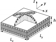
2. Structural Model
The middle surface Ω is assumed as the plate reference surface and a rectangular Cartesian reference frame (x, y, z) with (x, y) in Ω and z normal to Ω is assumed as reference system. The position of the upper+ and lower− surfaces of the kth layer are indicated as (k)z+ and (k)z−; the quantities that belong to a generic layer k are denoted with the superscript(k). The elastic displacements in the directions x, y and z are indicated with symbols u, v, w, respectively.
The through-the-thickness variation of displacements across the thickness is postulated as the sum of four separated contributions [
55]:
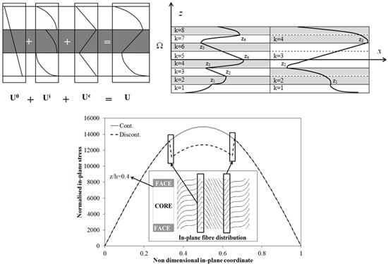
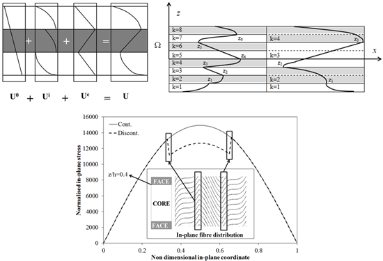
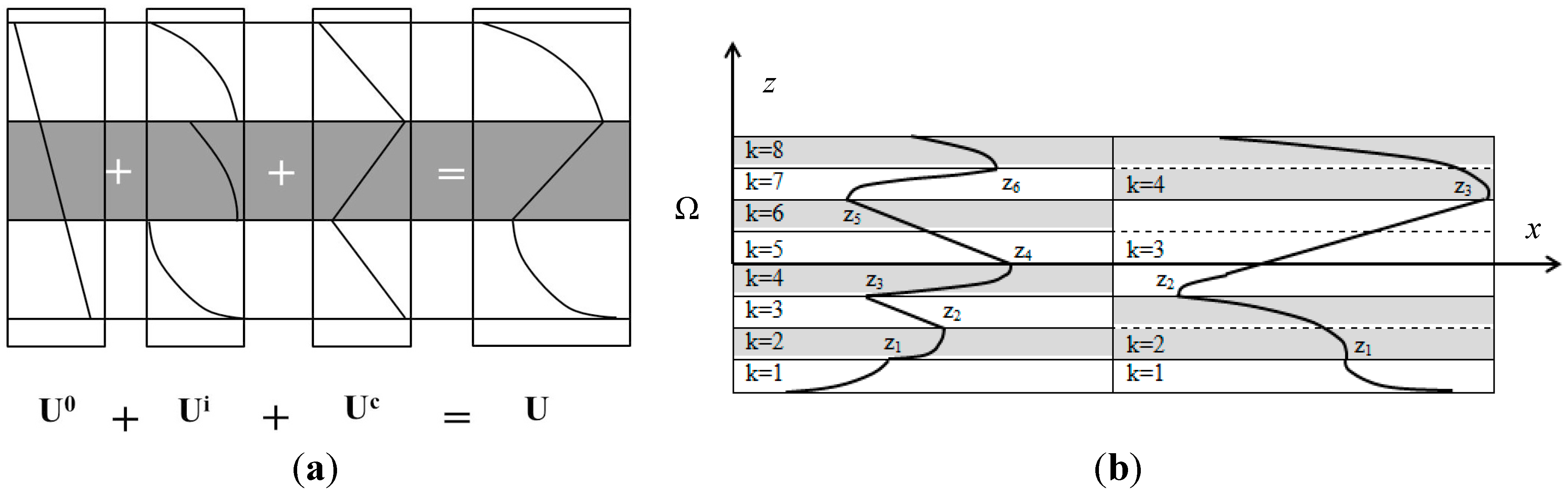
In order to make clearer the terms of Equation (1) their qualitative through-the-thickness variation for composite beams are reported in
Figure 1.
Figure 1.
(a) Through-the thickness variation of displacement contributions; (b) geometry considered to enforce in-plane continuity.
Figure 1.
(a) Through-the thickness variation of displacement contributions; (b) geometry considered to enforce in-plane continuity.
2.1. Basic Contribution Δ0
The contributions with superscript
0 that are indicated in compact form as
Δ0, contain just a linear expansion in
z that repeats the kinematics of the FSDPT model:
Having been used in so many applications, this part does not need further explanations. The displacements u0 (x, y), v0 (x, y), w0 (x, y) and the transverse shear rotations at the middle plane represent the functional d.o.f. of the zigzag model, in order to solve the structural problems with the minimal number of unknowns.
2.2. Variable Kinematics Contribution Δi
The contributions with superscript
i and symbol
Δi are terms whose representation can vary from point to point across the thickness:
These variable kinematics contributions are aimed at enabling a refinement across the thickness, in order to allow the model having the appropriate expansion order at any point, thus adapting to the local variation of solutions with the aim of accurately predict the stresses from constitutive equations. Owing to the correct representation of the strain energy achieved in this way, also accurate predictions of displacements are obtained.
The expressions of
Ax1…
Azn are determined as functions of the functional d.o.f. and of their spatial derivatives by enforcing the conditions:
Please notice that in this paper a comma is used to indicate differentiation, therefore for instance σzz,z represents the stress gradient σzz across the thickness. Likewise, the symbols (),x and (),y represent derivatives in x and y.
In addition, the equilibrium condition is imposed at discrete points across the thickness:
Thanks to these contributions and to the ones discussed forward, the transverse displacement is approximated with a high-order piecewise representation similar to that of in-plane displacements, determining the advantages discussed in the introductory section. As mentioned in the Introduction Section, this non-classical feature improves the predictive capability of the model since the transverse normal stress can play a primary role in keeping equilibrium in many cases.
The number of points at which indefinite equilibrium conditions Equation (8) are enforced depends on the expansion order considered. Indeed, a number of points np = Nlay ord_u − 2 have to be considered, Nlay being the number of computational layers and ord_u being the order of the expansion of displacements across the thickness. The position of the np points is chosen arbitrarily, paying attention to not consider points excessively near to the interfaces in order to avoid numerical problems (e.g., singular or badly scaled matrix). Indeed, as explained next, stress continuity conditions Equations (10) and (11) directly derive from equilibrium. Thus, imposing Equation (8) near to the interfaces could mean solving system with linearly dependent equations.
Numerical tests have shown that accurate results can always be obtained with just a third order expansion of the in-plane displacements, a fourth-order expansion of the transverse displacement and a number of computational layers across the thickness coincident with the number of physical layers. Accordingly, all the numerical results proposed in the paper will be obtained in this way.
Symbolic calculus is used to compute the expressions of Ax1…Azn through enforcement of physical constraints because the algebraic manipulations involved are rather cumbersome. In this paper all computation are carried out using MATLAB® symbolic software package.
No new displacement d.o.f. are incorporated during these operations, since symbolic calculus finds all expressions of Ax1…Azn in terms of the initially chosen d.o.f. u0, v0, w0, , and of their derivatives.
2.3. Zigzag Piecewise Contribution Δc
The expressions of the piecewise terms
Δc, which constitutes the zigzag contributions, are chosen as follows:
These terms are aimed at
a priori fulfilling the continuity of interlaminar stresses at the material interfaces, since they make the displacements continuous and with appropriate discontinuous derivatives in the thickness direction at the interfaces of physical and computational layers. In details, the two zigzag contributions
Φxk, Φyk are incorporated in order to satisfy:
The two zigzag contributions
Ψk,
Ωk are computed by enforcing:
which directly derive from the local equilibrium equations as a consequence of the continuity of transverse shear stresses.
The functions
Cuk,
Cvk and
Cwk are incorporated for making continuous the displacements at the points across the thickness where the representation is varied. Thus, their expressions in terms of the d.o.f. and of their derivatives are obtained at each interface of computational layers enforcing:
Like for Δi, in this case all the expressions of the continuity functions appearing in Equation (12) are also derived at each interface once for all using symbolic calculus, still being rather intricate expressions to manipulate.
2.4. Variable In-Plane Representation Δc_ip
In order to treat cases with material properties and/or lay-up that suddenly change moving along
x or
y, as it occurs using patches of different materials and across adherends and overlap of bonded joints, in this paper differently to [
55] it is supposed that the in-plane representation of displacements can vary. Such a variable representation is also necessary for treating different boundary conditions at different edges under the same analytical model.
The piecewise contributions Δc_ip are incorporated in order to make continuous the stresses and their gradients up the desired order at the interfaces of the regions where the in-plane representation is changed, which are here indicated as Θm. Notice that the d.o.f. u0, v0, w0, , formerly incorporated as the basic terms in Equation (2) already serve the purpose of making continuous the displacements u, v, w at Θm.
Because, in general, a different number of layers with different thickness and material properties could be found at Θ
m, the stress continuity should be enforced layer by layer at the right interfaces
S subdividing each physical layer in the right number of computational layers till the subdivisions match at the two sides of Θ
m (see, e.g.,
Figure 1b).
Contributions
Δc_ip to the displacements of the following type are incorporated in this paper:
where the summations are carried out at the
S interfaces mentioned above and the exponent of (
x −
xk)
n, (
y −
yk)
n is chosen in order to make continuous the stress gradient of order
n. For example, the continuity conditions
,
,
require just terms (
x −
xk), while the continuity of gradients
,
,
requires (
x −
xk)
2 and so on for higher-order gradients. Here the case of properties varying along
x is treated because just terms (
x -
xk)…(
x -
xk)
n are considered. Of course, when properties contemporaneously vary along
y, terms (
y −
yk)…(
y −
yk)
n should also be considered.
Thanks to its region-to-region variable representation, the present model can treat problems usually treatable only by a finite element scheme, becoming much more versatile than standard analytical models with a fixed representation.
As examples of the physical constraints that could be enforced, it is mentioned the case of clamped edges, for which equivalent single-layer models predict poor results because they are unable to account for a non-vanishing transverse shear while the three mid-plane displacements and the two shear rotations must vanish. In addition, of practical interest is the case of adhesively bonded joints with laminated adherends, which can be studied with the present displacement-based model, obtaining results as accurate as those obtained by the stress based models customarily used.
Applications to test cases (see, e.g., [
53,
55,
56,
57,
58,
71]) have proven that the present model can be used elsewhere, no special models being required for treating local geometry, loading and material variations. An applications to bonded joints having already been presented in [
71], in the numerical applications a sample case with clamped edges (Tessler, Di Sciuva and Gherlone [
72]) will be considered in order to show how non-classical boundary conditions can be easily satisfied.
However, the enforcement of all the physical constraints discussed above brings derivatives of the d.o.f. that are unwise for developing a finite element model, as discussed in the introductory section. Accordingly, a technique able to convert derivatives of any degree is developed and numerically assessed in the next sections, in order to give rise to a C0 equivalent model.
2.5. Equivalent C0 Model
The structural model of the former section is referred hereafter as the original model (OM), while its equivalent C
0 counterpart here developed as a refinement of the strain energy updating technique [
53,
54] is referred as the equivalent model (EM).
All the quantities that refer to OM are indicated with the superscript OM, while those referring to EM with the superscript EM. Therefore throughout this section the displacements appearing in Equation (1) are indicated as u(x, y, z)OM, v(x, y, z)OM, w(x, y, z)OM (in compact form ∀OM), while their counterparts obtained by the updating technique, which represent the equivalent C0 model, are indicated as u(x, y, z)EM, v(x, y, z)EM, w(x, y, z)EM (in compact form ∀EM). In a similar way, the strain energy of the model OM is indicated as SEOM, that of model EM as SEEM, and so on for all the other quantities.
The purpose of the strain energy updating technique (SEUPT) is to derive a modified expression ∀EM of displacements free from derivative of the d.o.f. through the energy balance, which makes equal strain energy, work of inertial forces and work of external forces of models OM and EM. The present refined version of SEUPT, whose peculiar features are discussed forward in this section, is developed with the purpose to be employed to construct computationally efficient finite elements with just the nodal d.o.f. of conventional shear-deformable plate elements and the predictive capability of layerwise plate elements.
It is postulated that the displacement field ∀
OM, can be expressed in a rearranged form
as the sum of expressions ∀
∅ that are just functions of the d.o.f. and expressions
containing the derivatives of the d.o.f.
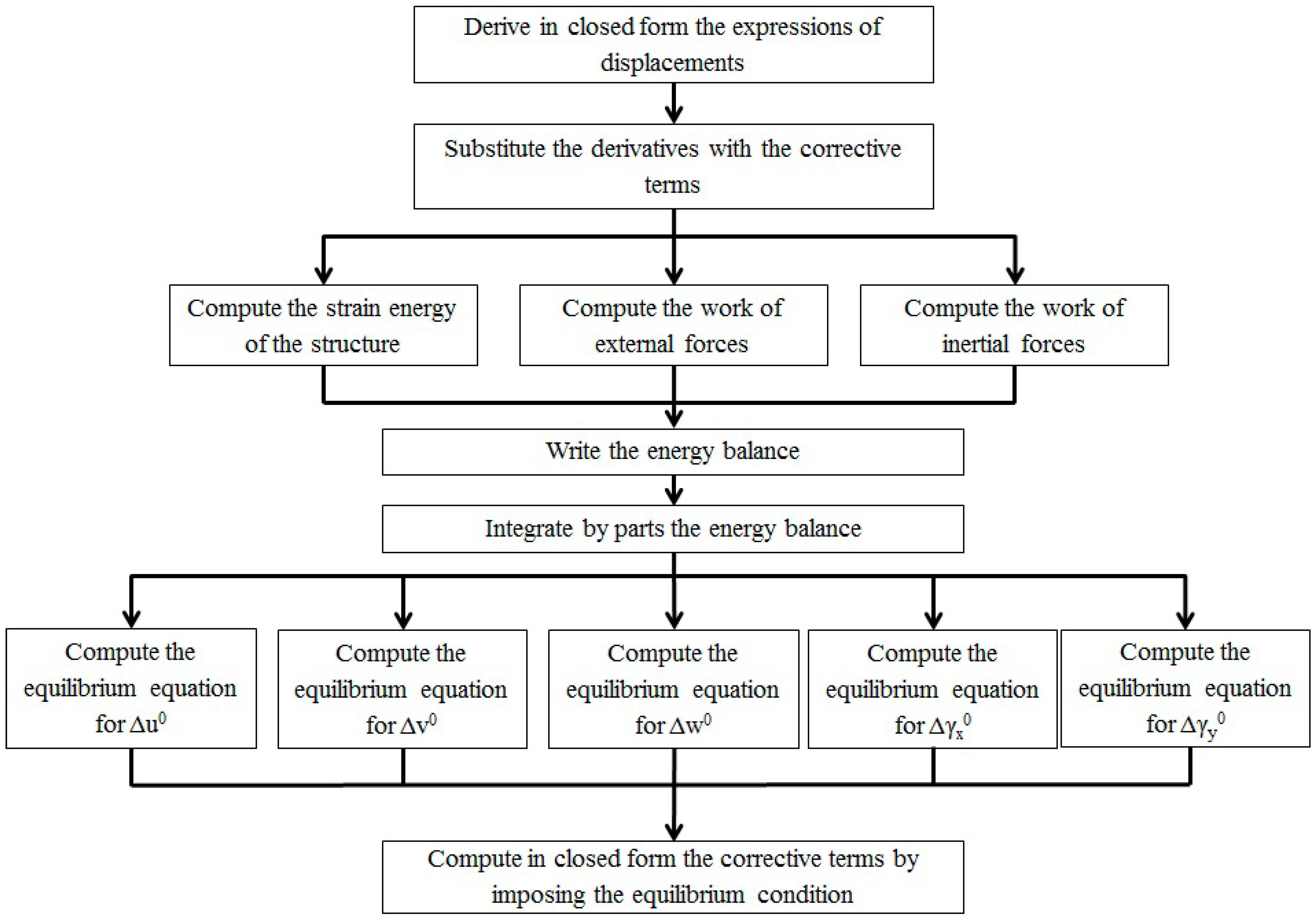
The steps for obtaining the model EM from the model OM are the following ones (see the flow chart of
Figure 2 for a synthesis).
- 1)
First, it is postulated that each derivative of the d.o.f appearing in
can be replaced by incorporating corrective terms ∆
u0, ∆
v0, ∆
w0, ∆
γx0, ∆
γy0 in ∀
∅, whose appropriate expressions will be derived from the energy balance. These corrective terms summed to each d.o.f.
u0,
v0,
w0,
,
, represent the variables of the equivalent model
*u0,
*v0,
*w0,
*,
* free from derivatives:
Figure 2.
Stages of the procedure employed to obtain the equivalent C0 model.
Figure 2.
Stages of the procedure employed to obtain the equivalent C0 model.
The appropriate expressions of the corrective terms will be obtained through the energy balance
= 0, which consists of the following contributions:
which represent respectively the strain energy
the work of external forces
and the work of inertial forces
as described forward. The symbols {
σij} and {
εij} represent the strain and stress vectors, respectively,
bi represents the body forces,
ti the surface forces,
ρ is the density and
ui are the displacements given by Equation (1) that are work conjugated to these forces of the OM model, or their counterparts of the EM model.
The previous equations giving the energy contributions are written in implicit form because their explicit form, which can be obtained in a straightforward, standard way substituting the expression of displacements of the model, cannot be reported being too lengthy.
The expressions of the energy contributions Equations (16)
i to (16)
iii contain derivatives of the displacement field variables that can be removed integrating by parts. Thus the energy balance Equation (16) can be split into five independent balance equations, one for each primary variable:
The previous symbols represent the energy contributions of the OM model. Their counterparts of the model EM are obtained substituting
u0,
v0,
w0,
,
with
u0,
*v0,
*w0,
*,
*.
- 2)
Once these five balance equations are written, they are used for obtaining the expressions of the five corrective terms ∆
u0, ∆
v0, ∆
w0, ∆
γx0, ∆
γy0 in a straightforward way. Indeed, each balance Equation (16)
iv should be either satisfied separately by the OM and EM models, or be used in order to equate separately the energy of each of the five contributions of the two models given by Equation (16)
iv under spatial distributions of the functional d.o.f. for the two problems,
i.e.,
u0,
v0,
w0,
,
and
u0,
*v0,
,
,
, respectively, under the same loading and boundary conditions. This constitutes the basic idea of SEUPT introduced in [
51,
52,
53,
54]. The difference is that the current version obtains once for all a closed form solution, thus it is no longer confined to the role of being a post-processing tool for improving the results of a finite element analysis carried out by standard shear-deformable elements, as the former version. The reason is that instead of using a spline interpolation of the nodal results, here an analytical general expression of the d.o.f. is used, as discussed forward, that enables obtainment of a solution in closed form, which can be used for developing C
0 finite elements. Each of the five expressions obtained equating the energy contributions Equation (16)
iv of the two models is here represented in implicit form as:
The five independent Equations (17) obtained from the energy balance can be used to compute the five unknowns ∆
u0, ∆
v0, ∆
w0, ∆
γx0, ∆
γy0 that define the updated displacement fields
*u0,
*v0,
,
,
of the C
0 model equivalent model EM.
The current version of SEUPT just requires to determine the expressions of the unknowns ∆
u0, ∆
v0, ∆
w0, ∆
γx0, ∆
γy0 once for all in closed form, instead of the numerical form used in [
51,
52,
53,
54]. As a result, the solution can be obtained in closed form and automatically using symbolic calculus. Since a direct solution instead of an iterative one is obtained, the processing time is speeded up with respect to the former version of SEUPT, which already appeared quite computationally efficient.
In order to find a solution from Equation (17), it is necessary to postulate how the d.o.f. vary in (x, y). Of course, when the solution of the structural problem can be found in closed form using trial functions defined over the whole domain, these functions can also be used for solving the updating problem. By this viewpoint, the trigonometric expansions considered in the sample cases reported in the numerical applications could be used. However it should be considered that in this case there is no need of removing the derivatives of the d.o.f., as they do not affect efficiency of the solving system. On the contrary, when the solution is found using a finite element scheme, the equivalent model EM is necessary to avoid use of inefficient high-order interpolation functions and displacement derivatives as nodal d.o.f. The present version of SEUPT is developed with the aim of being employed to create finite elements with just the nodal d.o.f. of classical efficient C0 shear deformable plate elements and the predictive capability of layerwise models.
Assume that the domain Ω is decomposed into subdomains, irrespectively of whether the problem will be solved by an analytic approach or via finite elements. In order to obtain from SEUPT a closed form solution once for all, an appropriate expression of the d.o.f. variation over a generic subdomain Ω* should be postulated, which allow a general solution in closed form. Though the numerical assessments will concern sample cases taken from the literature for which the solution can be found in closed form, in order to have the possibility to compare the solution of the OM and EM models free from errors inherent to the finite element scheme, here higher-order Hermite polynomials are considered. The order of these polynomials, which constitute the interpolation scheme employed to develop a conforming element from the model OM is determined by the order of derivation of each d.o.f. that is contained in the strain energy integral, which depends on the physical constraints enforced. Using these polynomials enables the continuity of the d.o.f. and of their derivatives till to the desired order at the bounds of the subdomains Ω*, so a regular solution is obtained in Ω by superposition. For example, a third-order expansion of the in-plane displacements and a fourth-order one for the transverse displacement give rise to third-order derivatives of the d.o.f. by the present model Equation (1) which requires a C2 continuity. Thus the d.o.f. should be expressed as the product of 5th order Hermite polynomials in
x and
y. Higher-order polynomials are required to ensure the continuity of stress gradients at the interfaces when an in-plane variable representation of the d.o.f. is assumed. The representation through Hermite polynomials constitutes the indefinite general solution of OM and EM irrespectively of the loading and boundary conditions, and it replaces the spline interpolation of finite element results for each specific case employed in the former version of SEUPT. Each d.o.f., represented by the symbol
, is expanded as the sum of Hermite’s polynomials
ρH
i in
x and
y as follows:
the index
i having been used to indicate the nodal values of
,
i.e., the values assumed at the vertices of the square sub-region Ω*, while the symbol
ρ has been used to indicate the specific polynomial related to a specific derivative of the d.o.f.
,
,
. Thus, the representation is continuous and has continuous derivatives inside Ω* and on its bound. Explicit terms have been reported only up to the second order of derivation, but additional similar terms can be included for obtaining the continuity also of higher-order derivatives.
Equating the energy of the OM model to that of the EM model corresponding to the representation Equation (18), the final expression of ∆u0, ∆v0, ∆w0, ∆γx0, ∆γy0 is obtained in closed form using symbolic calculus. This solution represents the C0 version of the model OM, since the arbitrary nodal values , , , of the d.o.f. (i.e., the values assumed at the vertices of the square sub-region Ω*) are converted into the equivalent ones form the standpoint of energy that do not contain derivatives.
As concluding observations, it is remarked that: (i) instead of defining each derivative of the d.o.f. itself as a new d.o.f., like it occurs with available techniques developed for achieving a C0 formulation, with the present technique the number of d.o.f. is kept fixed to five; (ii) being based on the search of an updated version of the functional d.o.f. free from derivatives that is equivalent by the energy standpoint to its consistent counterpart with derivatives, the current version of SEUPT can be used not only with the present structural model, but instead it can be used for updating any other model; and (iii) it is a useful technique in particular when the physical constraints concern stress gradients, since high order derivatives of the d.o.f are involved, that give rise to a large number of additional functional d.o.f. for achieving a C0 formulation with the other techniques.
3. Numerical Applications and Discussion
Numerical assessments will be presented with the aim of showing whether the present version of SEUPT provides an effective way for obtaining the EM C
0 equivalent version of the zigzag model OM [
55], without losing accuracy. It is reminded that in [
55] this model has been already proven to be accurate and computationally efficient when closed form solutions are considered, since it achieves the accuracy of layerwise models with just five d.o.f. Therefore, the aim of present numerical results is neither that of:
- a)
discussing the advantages of the zigzag modeling approach here used, nor discussing the advantages offered by its variable kinematics, as both aspects have been already comprehensively overviewed in [
43,
51,
52,
53,
54,
55,
56];
- b)
nor discussing the relative merits of a physically-based zigzag representation like the present one over the Murakami’s zigzag function just based upon kinematic assumptions, because both modeling options have been already compared and extensively discussed in [
17];
- c)
finally, nor comparing the available displacement-based and mixed theories incorporating zigzag functions to other existing models and nor to discuss their fidelity to 3D exact elasticity or finite element solutions, since assessments were already given among many others in the references quoted in [
17] that have shown their value.
Instead, the aim is just:
- d)
to assess the accuracy of the C0 equivalent EM model comparing its predictions to those of the OM model.
To reach this goal, as benchmark test cases multi-layered beams with simply-supported edges in cylindrical bending under sinusoidal transverse distributed loading are considered, which simulate laminated and sandwich beams with laminated faces. These apparently quite unrealistic test cases, owing to their loading and boundary conditions, are considered because the exact 3D elasticity solution is available, then it can be used as a reliable reference solution for comparing the predictions of EM and OM models. To this reason, these test cases are often considered in literature by researchers who assess the accuracy of available theories. Thus, in addition to exact results, also a large amount of approximate results by a variety of models is available for comparisons. Interest to these cases is also due to the possibility of obtaining results in closed form by the EM and OM models as Navier’s solutions, which do not suffer from round-off and discretization errors intrinsic of numerical solutions like finite elements. It could be observed that when analytical solutions can be found, as for the test cases here considered, there is no need of C0 models because the derivatives of the d.o.f. do not represent a drawback for this type of solution, while they are for finite elements. Thereby, analytical results by the EM model seam apparently meaningless, but instead they represent a necessary preliminary stage because before developing finite elements, the capability of the EM equivalent C0 model of preserving features and advantages of the OM model should be assessed.
The comparison between EM and OM models is extended also to damaged sandwich beams. The damage is simulated reducing the elastic moduli, according to the ply discount theory. Simply-supported, sandwich beams with damaged faces and/or core, undergoing sinusoidal transverse loading are considered and, in addition, the damage is assumed to be distributed over the entire length, because in this case the exact elasticity solution can be still found [
43] and used for comparisons. Owing to the reduction of elastic moduli used for simulating the damage rise, intricate through-the-thickness distributions of out-of-plane stresses take place as a consequence of asymmetric, distinctly different properties, which make the samples considered a very severe test case for the models.
Further objective is to assess whether the EM model preserves the accuracy of his counterpart OM model when variables stiffness properties are treated. Previous studies (see, e.g., [
53,
55,
56,
57,
58,
71]) have proven that the OM model is able to accurately and efficiently treat local geometry, loading and material variations. In particular, a successful application to adhesively bonded joints was presented in [
71] that demonstrated its capability of satisfying the quite complex stress-boundary conditions at the end of the overlap.
In order to show that the model EM preserves the capabilities of the OM model, an application will be presented to a laminate made of different constituent materials that requires a variable representation of the displacements. This case will show how the EM model can be used to efficiently convert all the d.o.f. derivatives consequent to the enforcement of the stress boundary conditions that are necessary for obtaining smooth solutions. As a further application, laminates incorporating curvilinear paths of fibers are considered. The sample cases presented in [
56] and [
58] using the OM model, which were obtained as the result of an optimization process aimed at finding the orientation at any point that minimizes the out-of-plane stresses at the critical interfaces, while maximizing the bending stiffness, are retaken in order to show the effectiveness of the equivalent EM model also in this case of practical interest.
As further assessment, the case of a cantilever beam will be considered in order to show how the EM model likewise the OM model can treat boundary conditions of practical interest that are difficult to satisfy.
3.1. Simply-Supported Edges and Sinusoidal Loading
As a preliminary assessment it is considered the simply supported <0°/90°/0°> laminated square plate analyzed in [
14,
61] and customarily considered as benchmark by many researchers. The constituent material has the following mechanical properties:
EL/
ET = 25;
GLT/
ET = 0.5;
GTT/
ET = 0.2; υ
LT = 0.25 each layer has the thickness equal to
h/3. Different length to thickness ratios are considered in
Table 1 where the stress field and the transverse displacement are reported normalized as follows:
The numerical results of
Table 1 show that the EM model is accurate and it does not suffer from locking.
Table 1.
Non-dimensional deflection and stresses of simply supported laminated <0°/90°/0°> plate under bi-sinusoidal loading.
Table 1.
Non-dimensional deflection and stresses of simply supported laminated <0°/90°/0°> plate under bi-sinusoidal loading.
![Aerospace 02 00637 i001]() |
|---|
| Lx/h | Model | w | σxx | σyy | σxy | σxz | σyz |
|---|
| 4 | Exact [14] | 2.006 | 0.755 | 0.556 | 0.0505 | 0.282 | 0.217 |
| Ref. [61] | 1.9597 | 0.7819 | 0.5195 | 0.051 | 0.2335 | 0.1885 |
| EM present | 1.9988 | 0.761 | 0.549 | 0.0508 | 0.275 | 0.212 |
| 10 | Exact [14] | 0.7405 | 0.59 | 0.288 | 0.0289 | 0.357 | 0.123 |
| Ref. [61] | 0.7316 | 0.596 | 0.2792 | 0.0288 | 0.3094 | 0.107 |
| EM present | 0.7402 | 0.591 | 0.285 | 0.0289 | 0.359 | 0.120 |
| 20 | Exact [14] | – | 0.552 | 0.2115 | 0.0234 | 0.385 | 0.094 |
| Ref. [61] | 0.5098 | 0.558 | 0.2088 | 0.0234 | 0.3286 | 0.084 |
| EM present | 0.5105 | 0.553 | 0.2110 | 0.0234 | 0.382 | 0.090 |
| 50 | Exact [14] | – | 0.541 | 0.185 | 0.0216 | 0.393 | 0.084 |
| Ref. [61] | 0.4439 | 0.5465 | 0.186 | 0.0218 | 0.3347 | 0.0766 |
| EM present | 0.4451 | 0.542 | 0.185 | 0.0216 | 0.390 | 0.085 |
| 100 | Exact [14] | 0.4347 | 0.539 | 0.181 | 0.0213 | 0.3947 | 0.083 |
| Ref. [61] | 0.4343 | 0.5448 | 0.182 | 0.0215 | 0.3355 | 0.0755 |
| EM present | 0.4346 | 0.538 | 0.181 | 0.0213 | 0.3949 | 0.083 |
3.2. Asymmetrical Cross-Ply Beam
As a subsequent test, it is considered the <0°/90°/0°/90°> asymmetrical cross-ply beam formerly analyzed in [
43,
60] having layers of equal thickness (0.25
h/0.25
h/0.25
h/0.25
h) and the mechanical properties of the constituent material equal to those of the previous case. Because the lay-up is asymmetrical, this sample case is suited to investigate whether the EM model provides accurate results, the stress fields being strongly asymmetrical too.
A length-to-thickness ratio of four being considered, which give rise to strong layerwise effects, several points should be considered across the thickness, in order to obtain accurate stress prediction from constitutive equations. This means that high-order terms should be considered in order to allow their coefficients to be determined by enforcing the indefinite equilibrium equations at some points across the thickness.
As already mentioned above, these results refer to an extremely thick case with a length-to-thickness ratio (
Lx/
h =
S) of 4 and simply-supported edges, undergoing a sinusoidal distributed transverse loading
Like in [
43] and [
60], in the present case, just a single component of the load,
i.e.,
M = 1 in Equation (20); is considered. Solution to this case is assumed as a series expansion as follow:
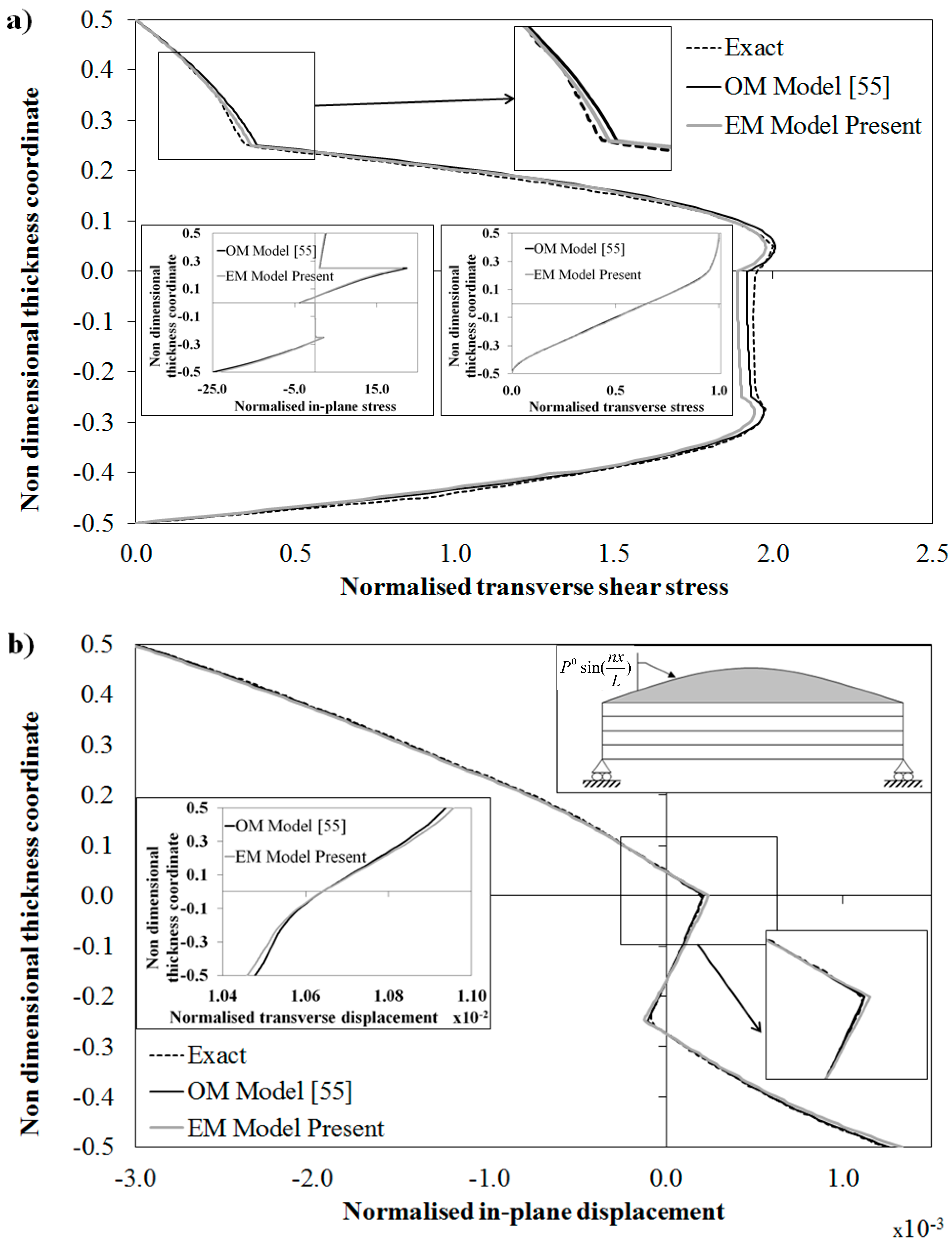
Figure 3.
Exact solution and through-the-thickness distribution of: (
a) normalized transverse shear stress; and (
b) normalized in-plane displacement by the OM Model [
55] and by the present EM Model for a laminated beam.
Figure 3.
Exact solution and through-the-thickness distribution of: (
a) normalized transverse shear stress; and (
b) normalized in-plane displacement by the OM Model [
55] and by the present EM Model for a laminated beam.
The trigonometric functions Equation (21) are chosen because they satisfy the simply-supported kinematic boundary constraint conditions
, whereas
Am,
Cm and
Dm constitute the unknown amplitudes. Once substituted in the governing equations, obtained applying the Rayleigh-Ritz method in standard form, the unknown amplitudes are computed in a straightforward way solving an algebraic problem. The results of
Figure 3 have been computed considering
M = 6 in Equation (21) and choosing a third order expansion of the in-plane displacement, a fourth-order expansion of the transverse displacement and a single computational layer for discretizing each physical layer. However, satisfactory results could even be obtained with
M = 1, as shown by the results of numerical test here not reported. For what concerns the computational time, the analysis with the model [
55] takes 3.96 s, while 4.01 s are required if the analysis is performed using the present EM model and 3.8 s are required when carrying out the analysis with FSDPT. It could be observed that the memory storage dimension is minimal, being almost the same of the FSDPT model, and that the processing time is also comparable, though an accurate 3D solution is obtained. It is reminded that nevertheless four different computational layers are considered, the number of functional d.o.f of the model does not increase. In the present case they are just three, like for the FSDPT model, since no variation rise in the
y direction. Of course, the overall number of d.o.f.,
i.e., the dimension of the algebraic system depends upon the expansion order chosen in Equation (21). In the present case it corresponds to a 18 × 18 system, having chosen
M = 6, while with
M = 1 it corresponds just to a 3 × 3 system.
The results of
Figure 3 are reported in the following normalized form:
Figure 3a represents the through-the-thickness variation of the shear stress
predicted by the OM model [
55] and by its equivalent C
0 counterpart EM, compared to the exact solution found in [
43] and [
60] applying the Pagano’s method [
13]. While
Figure 3b represents the through-the-thickness variation of the in-plane displacement
by the OM and the EM models and by [
43] and [
60]. These results show that the predictions of models OM and EM are in good agreement each and with the exact solution, thus demonstrating the effectiveness of the present technique in obtaining an equivalent C
0 model. It should be observed that the results of
Figure 3a are obtained directly from constitutive equations, thus as already shown in [
55], no post-processing techniques are required to obtain accurate results, as confirmed by the correct variation of the displacements of
Figure 3b. Note that the deviation between EM, OM and exact solution are more evident in the second layer, where the layerwise effects are stronger. This error could be reduced by further refining the representation of EM and OM through terms Equation (3). However, since deviations are lower than 5%, no refinements are adopted here, in order to keep lower computational effort.
3.3. Sandwich Beam
Now the sample case of a sandwich beam with asymmetrical properties is considered, in order to assess the quality of results provided by the EM model when the properties of the constituent layers are distinctly different.
It is here retaken the same sample case already considered in [
43], for which the exact 3D elasticity solution was obtained again applying the technique [
13]. Four constituent materials are considered, that are here indicated as MAT1 to MAT4, whose properties are reported hereafter. The face layers are made of materials MAT1 to MAT3, while the core is made of material MAT4. Thus, the sandwich beam is viewed as a 11-layer beam, having each face made of five layers, the lay-up sequence being chosen as (MAT 1/2/3/1/3/4)
s, with the following thickness ratios of the constituent layers (0.010/0.025/0.015/0.020/0.030/0.4)
s.
According to [
43], the following mechanical properties are chosen:
E1 =
E3 = 1 GPa,
G13 = 0.2 GPa, υ
13 = 0.25; MAT 2:
E1 = 33 GPa,
E3 = 1 GPa,
G13 = 0.8 GPa, υ
13 = 0.25; MAT 3:
E1 = 25 GPa,
E3 = 1 GPa,
G13 = 0.5 GPa, υ
13 = 0.25; MAT 4:
E1 =
E3 = 0.05 GPa,
G13 = 0.0217 GPa, υ
13 = 0.15. As it can be seen from these data, MAT1 is a rather compliant material, as compared to others, having weak properties in tension, compression and shear, MAT2 has high stiffness properties, MAT3 is stiff in tension and compression, but rather compliant in shear, while MAT4 as usual for core is very compliant. In this case, a length-to-thickness ratio (
Lx/
h =
S) of 4 is also considered.
The loading and boundary conditions, the series expansion used for representing the displacements Equation (21) and the normalization Equation (22) are still used.
Exact solution [
43] demonstrated that if the elastic moduli E
3 of the core and of the upper face layers are reduced by a factor 10
−2, strong layerwise effects rise due to asymmetry of properties and different moduli of adjacent constituent layers, thus making the out-of-plane stresses of this sample case difficult to capture. In particular,
shows an opposite behavior at the upper and lower face, which can be captured only if the models can be locally refined, e.g., by changing their representation across the thickness. Reduction of E3 implies a relevant increase of
in the upper face and in a region of the core close to it, while it decreases and changes sign at the lower face. Thus in order to treat this case, the models should be able to capture sudden variations. The results for this case obtained using the present structural model are reported in
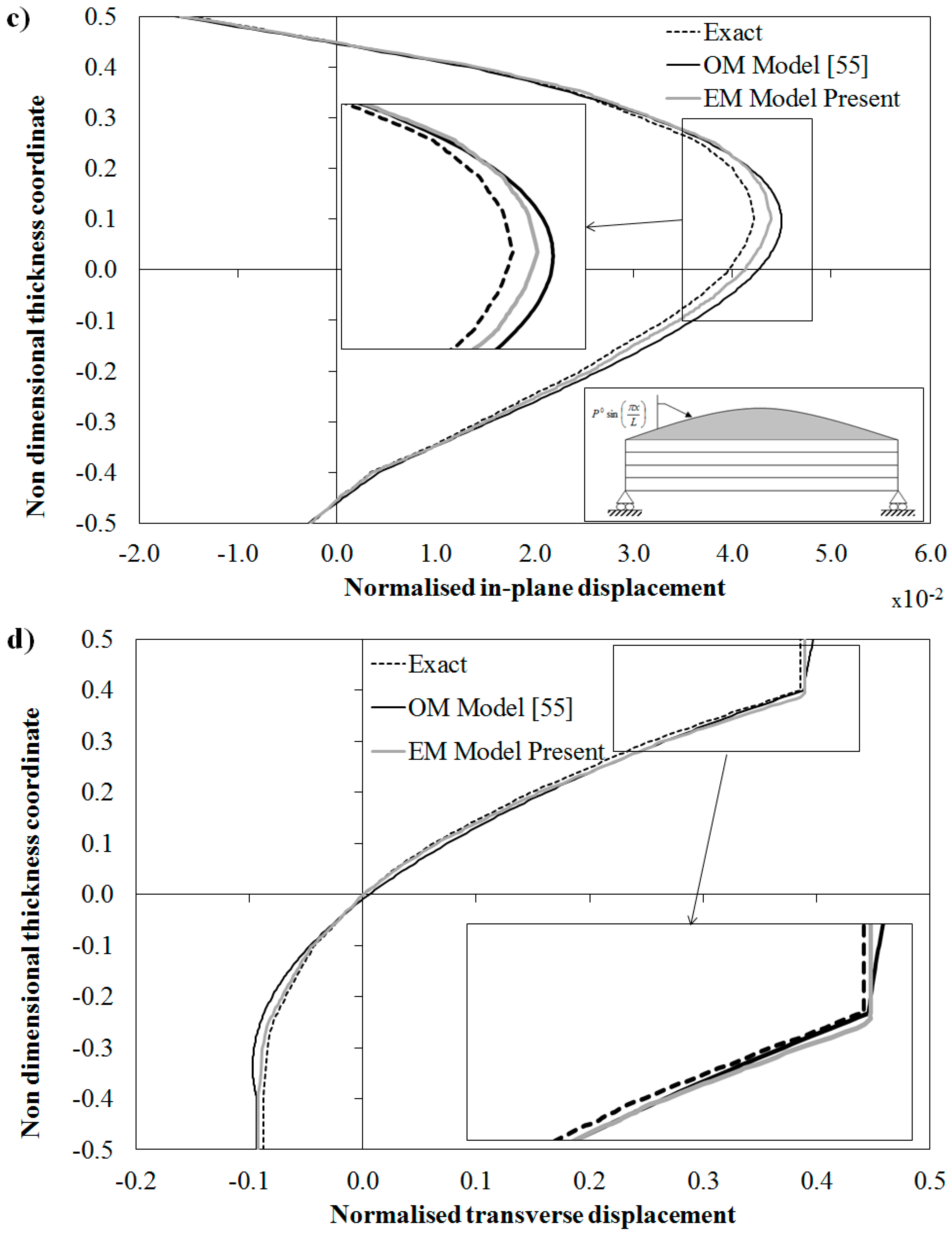
Figure 4 along with the exact solution.
The results of
Figure 4d, showing a strong variation across the thickness of
, point out that sandwiches require an accurate modeling of the transverse normal stress and deformation through a detailed description of the piecewise variation of the transverse displacement. The displacement of
Figure 4c also shows that the Murakami’s zigzag function [
49] based upon kinematic assumptions cannot appropriately represent the solution for this case, as the slope does not necessarily reverse at each interface, as shown by the exact solution. Thus, this could represent a further case where a physically based zigzag function should give better estimates, in addition to those discussed in [
44]. Note that deviations between EM, OM and exact solution are more evident in the core of the in-plane displacement, where the relatively poor mechanical properties of MAT4 enhance the deformability of the structure. As discussed above for
Figure 3a, this error could be reduced by further refining the representation of EM and OM through terms Equation (3). However, also for this case, no refinements are adopted here, in order to keep lower the computational effort, considering that deviations are still lower than 5%.
Figure 4.
Exact solution and through-the-thickness distribution of: (
a) normalized transverse shear stress; (
b) normalized transverse stress; (
c) normalized in-plane displacement; and (
d) normalized transverse displacement by the OM Model [
55] and by the present EM model for a sandwich beam with damaged upper face.
It can be seen from the results of
Figure 4 that the equivalent C
0 EM model gives as accurate results as the OM model also when the elastic modulus E
3 is reduced and, as a consequence, strong layerwise effects rise. In particular both models are shown to accurately predict the interlaminar stresses directly from constitutive equations even when the variations are rather intricate. The success of the EM model of this paper shows that a C
0 equivalent formulation can be obtained by SEUPT in order to overcome the derivatives of the d.o.f. that follows from the enforcements of the physical constraints inside any zigzag model.
3.4. Kinematics and Physically-Based Zigzag Functions
The test carried out in the previous section using a reduced E3 shows how the distributions of displacements and stresses can vary changing the properties of layers. This fact suggests that it could be quite hard to find appropriate a priori kinematic assumptions of general validity for the zigzag functions, while an always appropriate representation can be obtained with physically based zigzag functions like those employed for the OM and EM models. A further comparison among kinematically-based or physically-based zigzag functions is given next studying another test case.
Consider the sample case analyzed by Brischetto, Carrera and Demasi in [
73] dealing with a simply supported rectangular sandwich plate with a length to thickness ratio
Lx/
h = 4 and a length-side ratio
Ly/
Lx = 3 undergoing bi-sinusoidal loading. The two skins, which have a different thickness the ratios of upper (symbol us) and lower (symbol ls) faces and core (symbol c) being respectively
hls =
h/10;
hus = 2
h/10;
hc = 7
h/10 with respect to the thickness h of the plate, are made of different material. The constituent materials have the following mechanical properties:
Els/
Eus = 5/4,
Els/
Ec = 10
5, ν
ls = ν
us = ν
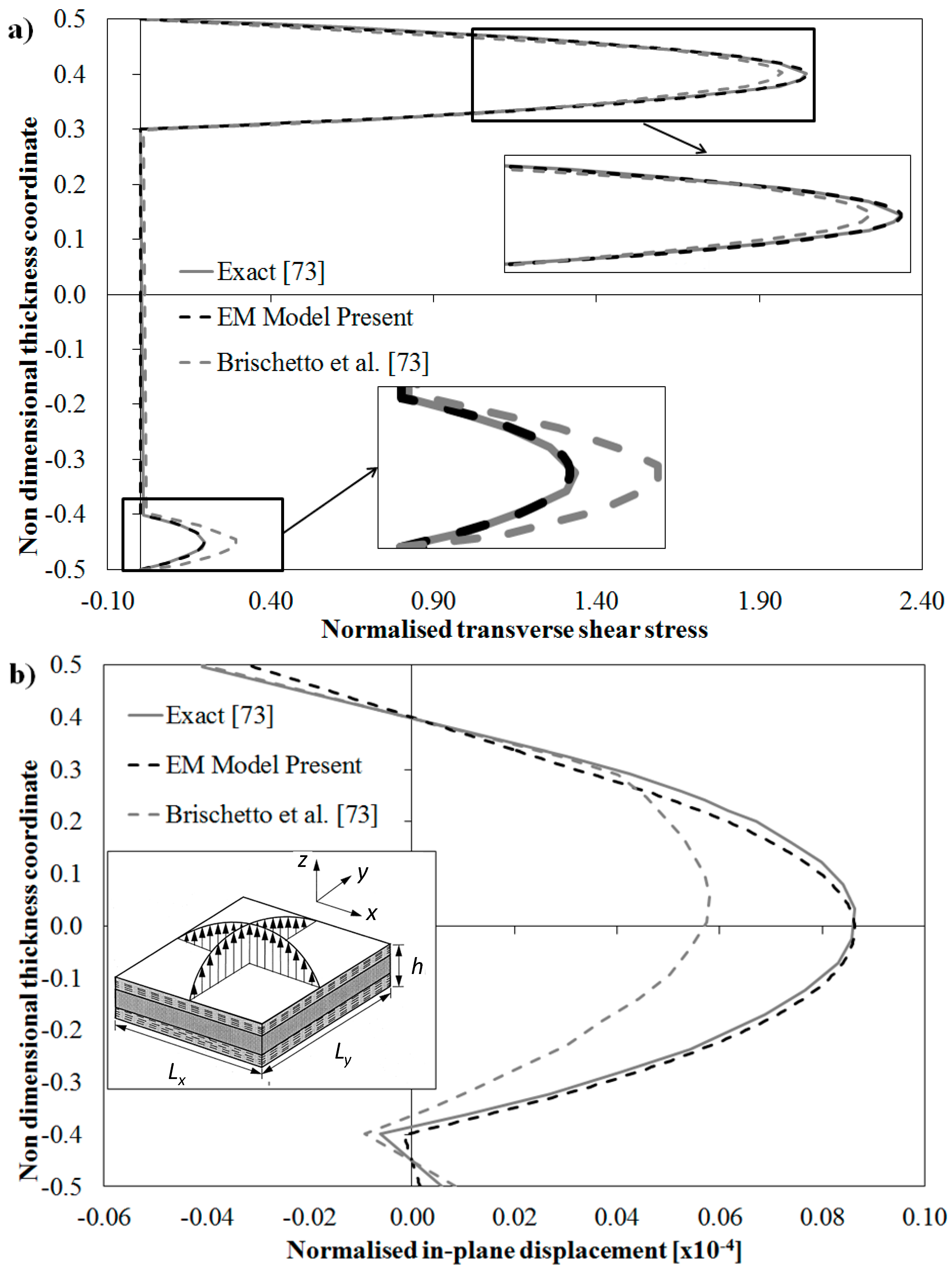
c = ν = 0.34. Owing to these asymmetrical, distinctly different geometric and material properties and to the high thickness ratio as well, strong layerwise effects rise making this sample case another severe test for the EM model. In addition, this model is of interest because the behavior of the physically based zigzag functions of the EM model can be compared with that of kinematic-based zigzag functions.
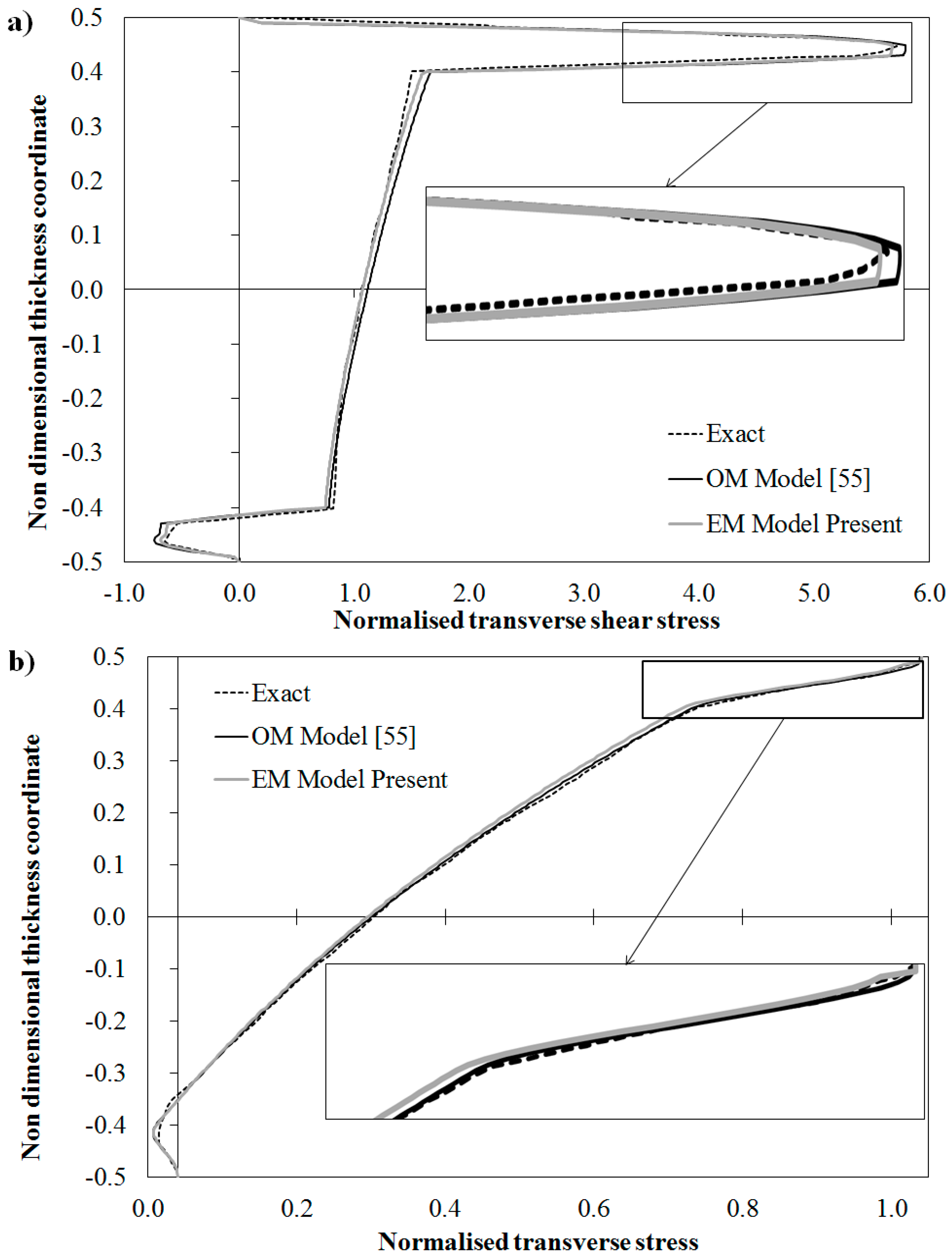
Figure 5 shows the comparison between the exact solutions for this test case presented in [
73] and the numerical results for this case predicted by the EM model and the model considered in [
73], which on the contrary of the EM model is based on use of Murakami’s zigzag function and a seventh order through-the-thickness representation. In
Figure 5a the variation of the transverse shear stress across the thickness is reported, while in
Figure 5b the variation of the in-plane displacement is given. According to [
73], these physical quantities are normalized as follows:
It can be seen that also for this case the EM model gives results always in a very good agreement with the exact 3D solution at any point, with the right gradients at the interfaces. Therefore it is confirmed that an accurate, equivalent C0 model can be constructed via SEUPT. As a measure of its efficiency, the processing time should be considered. To this regard it is reported that the entire process for the construction of the model, the computation of all coefficients and of continuity functions and for solution required just 6.028 s on a laptop computer.
As a reference result, the overall processing time required by the FSDT standard shear deformable model of 3.1 s on the same computer is reported. However it should be considered that the FSDT model that required a half of the time obtains totally wrong results, as it predicts a linear variation of the in-plane displacement and a piecewise linear, e.g., discontinuous and thus wrong transverse shear stress. No considerably better results are obtained for this stress when it is computed by integrating the local differential equilibrium equations. In this latter case the processing time was 4.06 s, thus close to that of the EM that on the contrary of the FSDT model always provides accurate results.
Figure 5.
Exact solution and through-the-thickness distribution of: (
a) normalized transverse shear stress and (
b) normalized in-plane displacement by the model [
73] and by the present EM model for a sandwich plate.
Figure 5.
Exact solution and through-the-thickness distribution of: (
a) normalized transverse shear stress and (
b) normalized in-plane displacement by the model [
73] and by the present EM model for a sandwich plate.
It is seen by the comparison with the reference solution [
73] obtained using the Murakami’s zigzag function, that the physically-based zigzag function by the EM model provides much more accurate results for the variation of the in-plane displacement across the thickness and only a little more accurate prediction of the shear stress, the reference model being already accurate for this quantity.
This result confirms that in some cases physically-based zigzag functions can be much accurate than their kinematics-based counterparts, as already focused in [
44], though the operations for developing models are much laborious and involve unwise derivatives of the displacements d.o.f. Because the EM model was shown to be accurate and efficient, SEUPT can be seen as a reliable tool for obtaining a C
0 model with physically-based zigzag functions suited for development of finite elements.
3.5. Clamped Edges
Because a distinctive feature of the OM model consists in the possibility of enforcing a non-vanishing transverse shear at clamped edges, where the mid-plane displacements and shear rotations must vanish, it should be tested whether this capability is preserved by the EM equivalent model. It could be noticed that once displacements and shear rotations are enforced to vanish within conventional models having the mid-plane displacements and shear rotations as functional d.o.f., a vanishing transverse shear is obtained that gives rise to poor results. On the contrary, the OM model can correctly enforce these boundary conditions because contributions Δi and Δc_ip can be determined by enforcing any desired set of boundary conditions, the coefficients appearing in these terms being computed through the enforcement of the desired conditions.
It is worthwhile to mention that the accuracy of the OM model in treating non-classical boundary conditions was already shown in [
71], considering a plate with a length to thickness ratio (
Lx/
h) of 5, that is simply supported on two opposite edges, clamped on the other two and it is undergoing a bi-sinusoidal normal load with intensity
p0 on the upper face, whereas the bottom one is traction free.
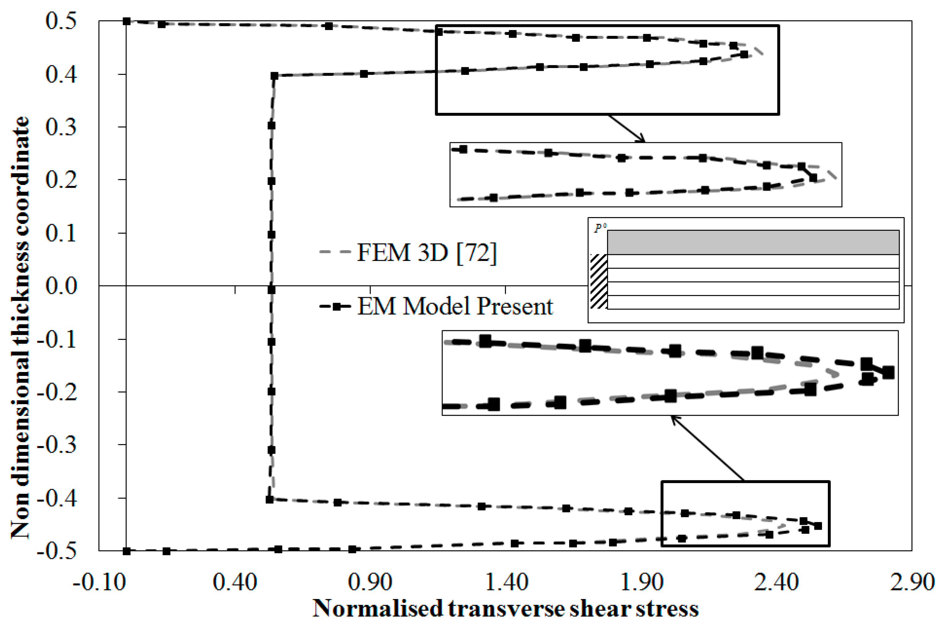
In order to assess whether the equivalent C
0 EM model can accurately describe the stress field with clamped edges, the cantilevered sandwich beam subjected to a uniform transverse loading of [
72] is considered. It has the faces made of unidirectional Carbon-Epoxy laminates (
E1 = 157.9 GPa,
E2 =
E3 = 9.584 GPa,
G12 =
G13 = 5.930 GPa,
G23 = 3.277 GPa, ν
12 = ν
13 = 0.32, ν
23 = 0.49) and a PVC foam core (
E = 0.1040 GPa, ν = 0.3) and a length-to-thickness ratio of 10, the thickness ratios of the constituent layers being 0.1
h/0.8
h/0.1
h.
According to [
72] the trial functions for the displacement d.o.f. are represented as products of orthogonal one-dimensional Gram–Schmidt polynomial in the
x and
y directions:
where
d is the generic d.o.f. (
i.e., {
d} = {
u0,
v0,
w0, γ
x0, γ
y0}),
are the unknown amplitude coefficients to be determined using the Rayleigh–Ritz method. According to [
72], the summations are truncated at
M = 7. The polynomials are as follow:
Figure 6 reports the through-the-thickness distribution of the transverse shear stress, which is normalized as follows:
Figure 6.
Normalized transverse shear stress by the present EM Model and by the 3D FEM [
72] for a cantilever beam.
Figure 6.
Normalized transverse shear stress by the present EM Model and by the 3D FEM [
72] for a cantilever beam.
Please notice that the results by the EM model are obtained employing three computational layers and enforcing the local equilibrium conditions at (−0.43h; −0.22h; −0.14h; 0; 0.09h; 0.23h; 0.44h).
The results show the OM model accurately predicts the through-the-thickness variation of the transverse shear stress at clamped edges. Being in a very good agreement with the results given in [
72], the equivalent EM model is still shown successful.
3.6. Variable Properties
Test cases with in-plane variable properties are here considered in order to assess whether the EM equivalent model preserves the capability of the OM model to treat these cases. Either a smooth continuous variation or a step variation are considered. The former case offers the possibility of showing how curvilinear paths of fibers can recover critical stresses. Many additional results are presented in [
56] and [
58] which show how this result can be achieved preserving a high bending stiffness. The latter case is considered in order to show how coefficients
Δc_ip can make continuous the stresses and their gradients up the desired order at the interfaces of the regions where properties suddenly change.
3.7. Smooth Variation
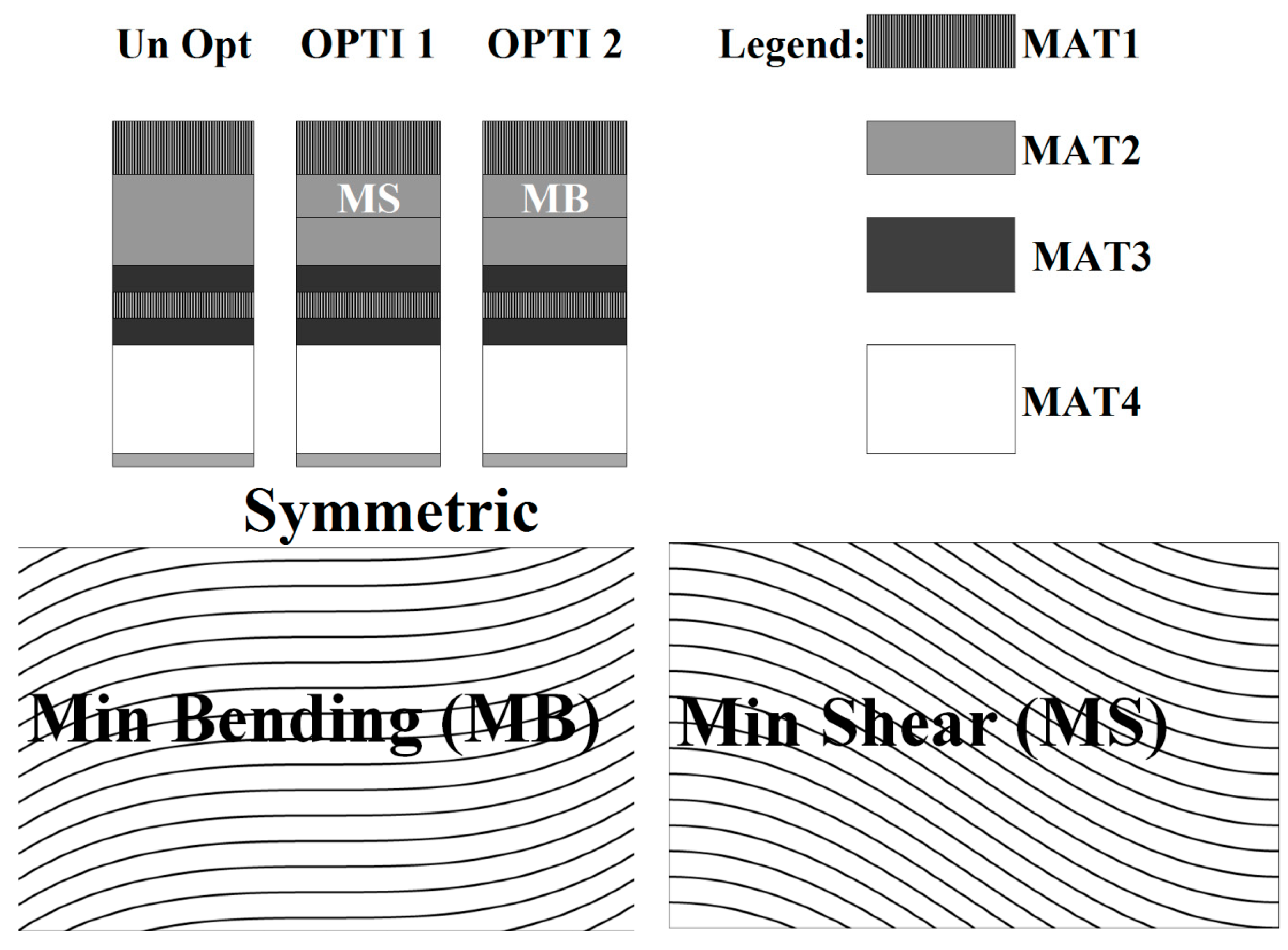
The curvilinear paths of fibers considered were obtained in [
58] as the solution of the Euler–Lagrange equations obtained by enforcing the contemporaneous extremization of the strain energy in bending and transverse shear under variation of the stiffness properties. The goal was to find a proper distribution of the stiffness properties that minimizes the energy absorbed through unwanted modes involving interlaminar strengths and maximizes that absorbed by modes involving membrane strengths. As a result, this process transfers energy from bending and shear to membrane modes through a suited distribution of stiffness properties that constitute the curvilinear paths of fibers. Coupling plies with opposite properties, the out-of-plane stress concentrations can be recovered at the critical interfaces without any stiffness loss. These plies, here referred to as Min Bending (MB) and Min Shear (MS) plies, are represented in
Figure 7. MB is characterized by a significant increase of
Q11 at the center of the ply, and a reduction at its edges. The local in-plane shear stiffness
Q12 is significantly higher at bounds of the ply than at the center, where it is equal to that of the straight-fiber case. This trend is also the same of the stiffness coefficient
Q22. As a result, plies MB contribute to give an increase of the bending stiffness at the center of a laminate and a decrease at the bounds, where the shear stiffness in the in-plane direction grows. The opposite occurs with MS. It could be observed that curvilinear paths of fibers similar to MB and MS from [
58] have been obtained by other researchers using different optimizations techniques (see, e.g., Khani
et al. [
4] and Nik
et al. [
7]).
Figure 7.
Lay-ups and fiber orientation considered.
Figure 7.
Lay-ups and fiber orientation considered.
In the numerical applications it is considered the case of a double-core sandwich beam undergoing a sinusoidal loading, with a length-to-thickness ratio of 4. It is made of the same constituent materials as in the former case,
i.e., materials MAT 1 to MAT 4 are considered. The stacking sequence is a (MAT 1/2/3/1/3/4/2)
s and the following thickness ratios of the constituent layers (0.010/0.025/0.015/0.020/0.030/0.4/0.01)
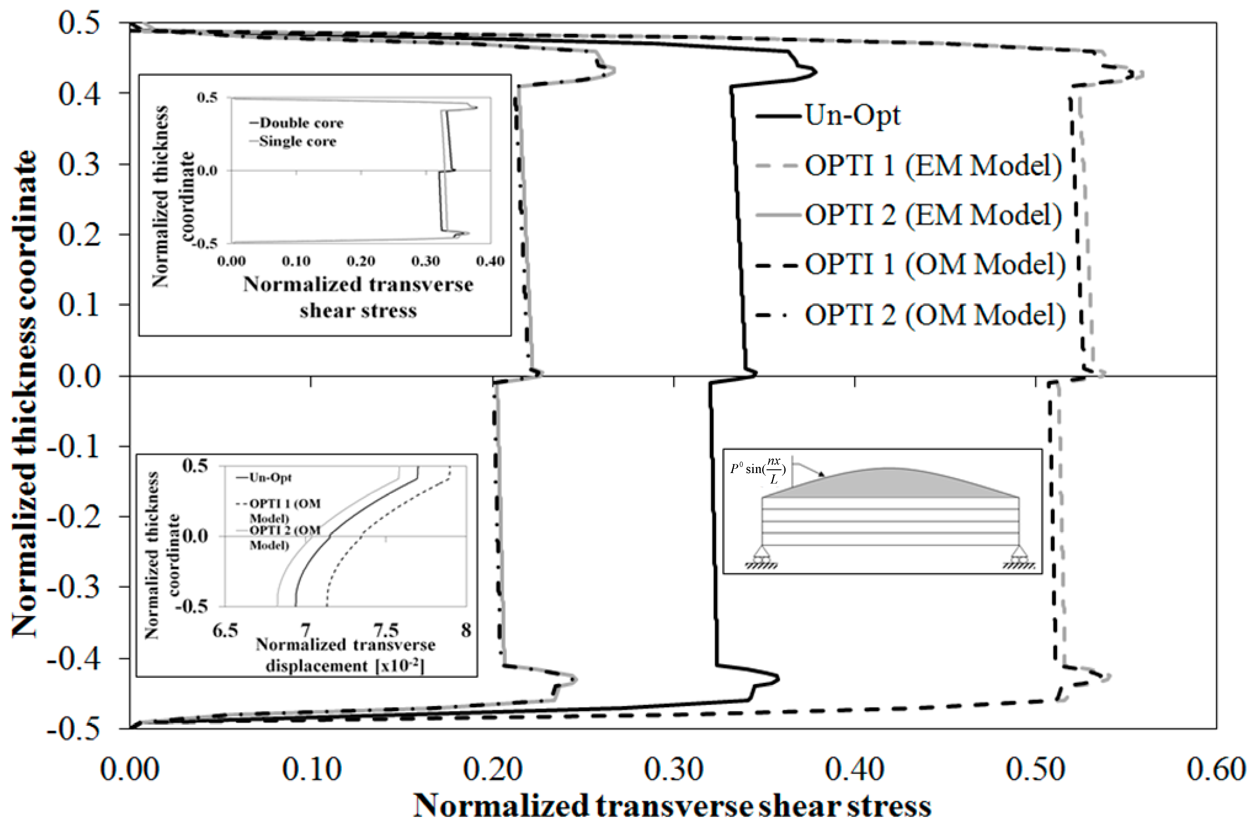
s is considered. Like in the former case, the sandwich beam is simulated as a multilayered beam. The results for this reference case are referred as Un-Opt in
Figure 8, where the through-the-thickness variation of transverse shear stress, normalized according to Equation (22), is reported. The results by the EM model are indicated as OPTI 1 SEUPT and OPTI 2 SEUPT. Of course, the aim being to assess the behavior of the EM model with curvilinear paths of fibers, the result with straight-fibers by the EM model is omitted. Lay-ups OPTI 1 and OPTI 2 are obtained from the straight-fiber case Un-Opt by incorporating a layer of type MB or MS having a thickness that is a half of the thickness of layer in MAT2. As an inset, the comparison with a single-core sandwich beam with the same outer faces is reported showing that the core is a little less stressed than its counterpart, while faces are a little more stressed (straight-fibers case). As shown in [
59], the advantage of double-core sandwiches over their single-core counterparts is that they can bear the stresses due to loading also when failed because the intermediate face inhibits the deleterious spreading of failure and damage. Thus, although the intermediate face does not contribute to the bending stiffness, it does not necessarily increase the weight, because the single-core needs to be over-sized in order to tolerate the damage.
Figure 8 shows that the EM model obtains results always in a good agreement with those by the OM model also when variable-stiffness faces are considered (results are normalized as in Equation (22)). As a further test, next a sudden variation of properties is considered.
Figure 8.
Normalized transverse shear stress by the OM Model and by the present EM Model for a simply-supported double core sandwich beam with spatially variable stiffness faces.
Figure 8.
Normalized transverse shear stress by the OM Model and by the present EM Model for a simply-supported double core sandwich beam with spatially variable stiffness faces.
3.8. In-Plane Step Variation of Properties
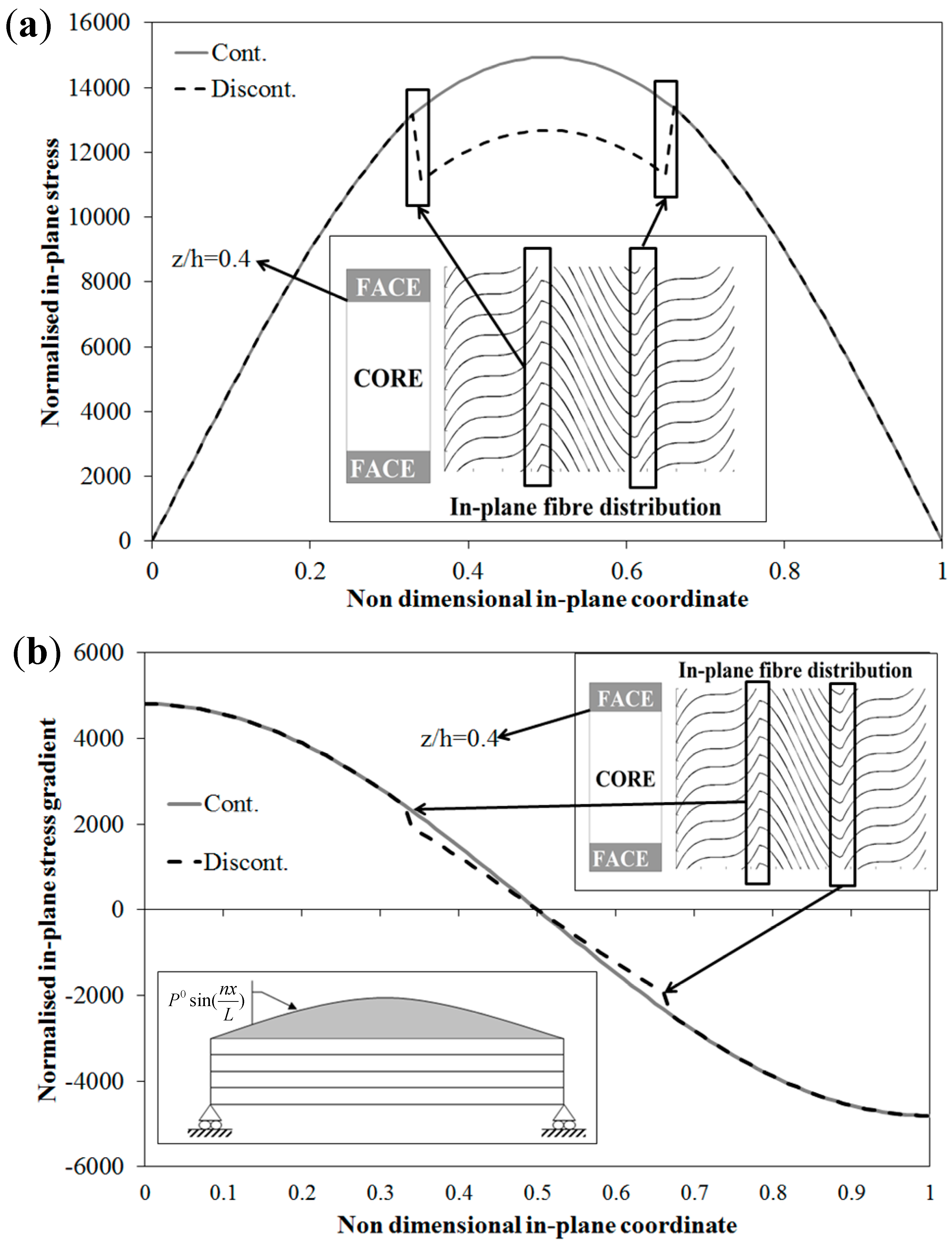
The sample case now considered is again that of a sandwich beam undergoing distributed sinusoidal loading. The structure is simulated as a three-layer beam, the faces being the outer layers, which are assumed to be made of an homogenous, orthotropic material with elastic moduli E1 = 25 GPa, E3 = 1 GPa, G13 = 0.5 GPa, υ13 = 0.25, and the core being the inner layer, which is assumed as an homogeneous isotropic material with E1 = E3 = 0.05 GPa, G13 = 0.0217 GPa, υ13 = 0.15.
Because the purpose is to show the capability of the EM model to achieve continuous in-plane stress distributions across the interfaces of regions where the elastic properties suddenly change, e.g., when patches are used for repairing damage, or as a result of optimization studies aimed at achieving specific local properties without use of curvilinear paths of fibers, a length-to-thickness ratio of 10 is considered that gives rise to sufficiently large bending deformations. Thus, in this case, attention is focused on the bending stress,
i.e., the in-plane stress
at
z /
h = 0.4. The faces are assumed to be 2 mm thick, while the core is 6 mm thick.
Figure 9 shows how the principal material orientation 1 is assumed to vary along the span. It can be seen that such orientation angle suddenly changes at the two interfaces
x/
Lx = 1/3 and
x/
Lx = 2/3, while it smoothly varies elsewhere. Three regions are considered where face plies of type MB or MS are used, then at the interfaces of these regions the material orientation angle suddenly changes.
Figure 9.
Sandwich beam with step variation of fiber orientation: non-dimensional in-plane variation of (a) in-plane stress and (b) in-plane stress gradient.
Figure 9.
Sandwich beam with step variation of fiber orientation: non-dimensional in-plane variation of (a) in-plane stress and (b) in-plane stress gradient.
If one carries out the analysis with the OM model not properly setting the continuity functions
to
in Equation (13),
i.e., not enforcing the continuity of the stress
and of its gradients in
x, a discontinuous wrong stress distribution of
is obtained by the equivalent EM model at the interfaces along the span, as shown in
Figure 9, while setting these functions in the proper way the right smooth variation is obtained. It is worthwhile to mention that in this case, in order to restore the in-plane continuity of the membrane stress gradient, it is sufficient to consider continuity functions up to the third order in
x. This is due to the fact that the difference between the stiffness coefficients at the interfaces is rather mild.
Thus, the results of
Figure 9 show the capability of the C
0 equivalent model EM to correctly predict the stresses even when the material properties suddenly vary in the in-plane directions. This is a direct consequence of the capability of the OM model to treat in-plane discontinuities, as shown in [
71]. Again the results have shown that the EM model preserves features and advantages of the OM model.


