Acoustic Radiation by 3D Vortex Rings in Air

Abstract

Acoustic radiation emitted by three-dimensional (3D) vortex rings in air has been investigated on the basis of the unsteady Navier–Stokes equations. Power series expansions of the unknown functions with respect to the initial vorticity which is supposed to be small are used. In such a manner the system of the Navier–Stokes equations is reduced to a parabolic system with constant coefficients at high derivatives. The initial value problem is as follows. The vorticity is defined inside a toroid at t = 0. Other gas parameters are assumed to be constant throughout the whole space at t = 0. The solution is expressed by multiple integrals which are evaluated with the aid of the Korobov grids. Density oscillations are analyzed. The results show that the frequency band depends on the initial size of the vortex ring and its helicity. The presented data may be applied to the study of a flow in a wake region behind an aerodynamic body.

1. Introduction

Vortical structures (vortex rings and cylindrical vortices) play an important role in the sound radiation of gaseous flows. These structures convert a fraction of their rotational energy into sound waves [1]. The case of the three-dimensional (3D) vortex is of special interest. In this case we have three velocity components ($v_r,v_{\phi },v_{\theta }$), with $r,\phi ,\theta$ being spherical coordinates. The aim of the present investigation is to determine the frequency band of acoustic radiation emitted by 3D vortex rings in air. The analysis is based on the unsteady Navier–Stokes equations. A new method for solving the equations is set forth. It uses power series expansion of the unknown functions with respect to the initial vorticity which is supposed to be small. By applying this procedure the Navier–Stokes equations are reduced to a parabolic system with constant coefficients. As a result we get the solution in the form of a power series, with multiple integrals being appropriate coefficients. The first term of the series is the main one that determines the properties of acoustic radiation at small vorticity. General questions of sound generation by vortex structures were considered in [2,3]. Acoustic radiation by a solitary vortex ring in incompressible and weakly compressible fluid was analyzed in [4]. There are investigations of the acoustic radiation during the interaction of two vortex rings [5,6]. Linear problems of sound production by vortices are considered in [1]. The influence of vortex rings on properties of turbulent flows is confirmed by numerous experiments [7,8] and by computations [9,10]. Nevertheless, further investigations are necessary in the field of acoustic radiation by a solitary vortex ring in viscous heat-conducting gas. The topic of this paper is the study of the frequency band of acoustic radiation by a 3D solitary vortex ring in air and the evolution of the radiation.

2. Governing Equations

We use the Helmholtz decomposition of the velocity field as a potential part and a solenoidal one:

$$\begin{array}{c}v\left(x,t\right)=-\frac{\nabla }{4\pi }{\displaystyle {\int }_{R^3}\frac{s\left(\xi ,t\right)}{\left|x-\xi \right|}d\xi }+\frac{\nabla }{4\pi }\times {\displaystyle {\int }_{R^3}\frac{\mathrm{\Omega }\left(\xi ,t\right)}{\left|x-\xi \right|}d\xi ,}\\ s=\nabla v,\mathrm{\Omega }=\nabla \times v,\nabla =\left\{\frac{\partial }{\partial x_1},\frac{\partial }{\partial x_2},\frac{\partial }{\partial x_3}\right\}\end{array}$$

(1)

Taking into account Equation (1), the Navier–Stokes equations in dimensionless form can be written as follows:

$$\begin{gathered} \frac{\partial {\mathrm{\Omega }}_i}{\partial t}=\nu \Delta {\mathrm{\Omega }}_i+\frac{3}{4}{\epsilon }_{ijl}\nu \left(\frac{\partial v_l}{\partial x_m}+\frac{\partial v_m}{\partial x_l}\right)\frac{{\partial }^{2}h}{\partial x_j\partial x_m}-v_j\frac{\partial {\mathrm{\Omega }}_i}{\partial x_j}+{\mathrm{\Omega }}_m\frac{\partial v_i}{\partial x_m}+f_{1i}, \\ \frac{\partial w}{\partial t}=-v_j\frac{\partial w}{\partial x_j}+s, \\ \frac{\partial s}{\partial t}=\frac{1}{\gamma }\exp \left(h\right)\Delta w+\frac{4}{3}\nu \Delta s-\left(\frac{1}{\gamma }\exp \left(h\right)+0.5\nu s\right)\Delta h-v_j\frac{\partial s}{\partial x_j}+1.5\nu \frac{\partial v_i}{\partial x_j}\frac{{\partial }^{2}h}{\partial x_i\partial x_j}+f_2, \\ \frac{\partial h}{\partial t}=\frac{\gamma }{\mathrm{Pr}}\eta \Delta h-\left(\gamma -1\right)s-v_j\frac{\partial h}{\partial x_j}+f_3, \\ \Delta =\frac{{\partial }^2}{\partial x_j\partial x_j},w=-log\rho ,h=logT,\nu =\mu /\rho ,\eta =\lambda /\rho ,i=1,2,3;j=1,2,3;l=1,2,3;m=1,2,3 \end{gathered}$$

(2)

Here, ${\epsilon }_{ijl}$ is the antisymmetrical tensor; $\rho ,T,v$ are the dimensionless density, temperature, velocity (divided by ${\rho }_0,T_0,c_0,$ respectively); $\mu ,\nu ,\lambda ,c$ are the viscosity, kinematic viscosity, heat conductivity, and low-frequency sound speed; $\gamma$ is the adiabatic exponent; Pr is the Prandtl number. The functions $f_{1i},f_2,f_3$ are non-linear terms with respect to the first derivatives over coordinates. Subscript “0” refers to the initial state. The system Equation (2) was made dimensionless by using the characteristic length $l_0={\nu }_0/c_0$ and the characteristic time $t_0={\nu }_0/c_0^2.$

2.1. Initial Value Problem

At the initial instant the vorticity has non-zero values only within a gaseous toroid [11]:

$$\begin{array}{c}{x}_1=\left(r_{00}{u}_1\sin u_2+R_c\right)\cos u_3,x_2=\left(r_{00}{u}_1\sin u_2+R_c\right)\sin u_3,x_3=r_{00}{u}_1\cos u_2,\\ 0<u_1<1,0<u_2,u_3<2\pi ,\end{array}$$

(3)

$r_{00},R_c$ being the initial dimensions of the vortex ring, namely $r_{00}$ is the radius of its cross-section, $R_c$ is the radius of the ring. The problem is considered under the assumption that the dimensionless initial vorticity ${\omega }_0$ is small: ${\omega }_0<<1.$ The initial conditions are

$${\mathrm{\Omega }}_1=-{\omega }_0\sin u_3,{\mathrm{\Omega }}_2={\omega }_0\cos u_3,{\mathrm{\Omega }}_3=\alpha {\omega }_0$$

(4)

inside the initial toroid,

$$w\left(x,0\right)=s\left(x,0\right)=h\left(x,0\right)=0$$

(5)

in the whole space. The parameter $\alpha$ refers to helicity. The value of $\alpha$ is $\alpha =0$ (no helicity) and $\alpha =1$ (there is the presence of helicity).

2.2. Solution to the Problem

Equation (2) represents a non-linear parabolic system. We seek the solution of the parabolic system as a power series expansion. Taking into account Equation (1) and the initial conditions, we get:

$$\begin{array}{l}{\mathrm{\Omega }}_i\left(x,t\right)=\epsilon {\mathrm{\Omega }}_i^{\left(1\right)}\left(x,t\right)+{\epsilon }^2{\mathrm{\Omega }}_i^{\left(2\right)}\left(x,t\right)+{\epsilon }^3{\mathrm{\Omega }}_i^{\left(3\right)}\left(x,t\right)+\mathrm{...}\\ v_i\left(x,t\right)=\epsilon v_i^{\left(1\right)}\left(x,t\right)+{\epsilon }^2{v}_i^{\left(2\right)}\left(x,t\right)+{\epsilon }^3{v}_i^{\left(3\right)}\left(x,t\right)+\mathrm{...}\end{array}$$

(6)

Inserting Equation (6) into Equations (1) and (2) gives

$$\begin{gathered} w\left(x,t\right)={\epsilon }^2{w}^{\left(1\right)}\left(x,t\right)+{\epsilon }^3{w}^{\left(2\right)}\left(x,t\right)+{\epsilon }^4{w}^{\left(3\right)}\left(x,t\right)+\mathrm{...} \\ s\left(x,t\right)={\epsilon }^2{s}^{\left(1\right)}\left(x,t\right)+{\epsilon }^3{s}^{\left(2\right)}\left(x,t\right)+{\epsilon }^{\left(4\right)}{s}^{\left(3\right)}\left(x,t\right)+\mathrm{...} \\ h\left(x,t\right)={\epsilon }^2{h}^{\left(1\right)}\left(x,t\right)+{\epsilon }^3{h}^{\left(2\right)}\left(x,t\right)+{\epsilon }^4{h}^{\left(3\right)}\left(x,t\right)+\mathrm{...} \end{gathered}$$

(7)

We have for the lowest-order functions:

$$\frac{\partial {\mathrm{\Omega }}_i^{\left(1\right)}}{\partial t}=\Delta {\mathrm{\Omega }}_i^{\left(1\right)},$$

$$\frac{\partial w^{\left(1\right)}}{\partial t}=s^{\left(1\right)},$$

$$\frac{\partial s^{\left(1\right)}}{\partial t}=\frac{1}{\gamma }\Delta w^{\left(1\right)}+\frac{4}{3}\Delta s^{\left(1\right)}-\frac{1}{\gamma }\Delta h^{\left(1\right)}+{\psi }_3^{\left(1\right)},$$

(8)

$$\frac{\partial h^{\left(1\right)}}{\partial t}=\frac{\gamma }{\mathrm{Pr}}\Delta h^{\left(1\right)}-\left(\gamma -1\right)s^{\left(1\right)}+{\psi }_4^{\left(1\right)},$$

$${\psi }_3^{\left(1\right)}=\frac{\partial v_m^{\left(1\right)}}{\partial x_j}\frac{\partial v_j^{\left(1\right)}}{\partial x_m},{\psi }_4^{\left(1\right)}=\frac{1}{2}\gamma \left(\gamma -1\right)D_{mj}{v}^{\left(1\right)}{D}_{mj}{v}^{\left(1\right)},D_{mj}{v}^{\left(1\right)}=\frac{\partial v_m^{\left(1\right)}}{\partial x_j}+\frac{\partial v_j^{\left(1\right)}}{\partial x_m}$$

From Equation (1) one deduces:

$$\begin{array}{c}{v}^{\left(1\right)}\left(x,t\right)=-\frac{0.03125}{{\pi }^{5/2}{t}^{3/2}}{\displaystyle {\int }_{R^3}d\xi {\displaystyle \underset{0}{\overset{\infty }{\int }}d{r}^{\prime }}{\displaystyle \underset{0}{\overset{\pi }{\int }}\sin {\theta }^{\prime }d{\theta }^{\prime }{\displaystyle \underset{0}{\overset{2\pi }{\int }}d{\phi }^{\prime }{\mathrm{\Omega }}^{\left(1\right)}\left(\xi ,0\right)\times n}}}\exp \left(-\frac{0.25}{t}{\left|x+x^{\prime }-\xi \right|}^2\right),\\ n=\left\{\sin {\theta }^{\prime }\cos {\phi }^{\prime },\sin {\theta }^{\prime }\sin {\phi }^{\prime },\cos {\theta }^{\prime }\right\},x^{\prime }=\left\{r^{\prime }\sin {\theta }^{\prime }\cos {\phi }^{\prime },r^{\prime }\sin {\theta }^{\prime }\sin {\phi }^{\prime },r^{\prime }\cos {\theta }^{\prime }\right\}\end{array}$$

(9)

The system Equation (8) consists of three homogeneous parabolic equations with respect to ${\mathrm{\Omega }}_i^{\left(1\right)}$ and a non-homogeneous parabolic subsystem. All equations have constant coefficients at higher derivatives. The solution to the subsystem can be obtained with the aid of the Fourier transform.

The first Equation (8) yields

$${\mathrm{\Omega }}_i^{\left(1\right)}\left(x,t\right)=\frac{0.125}{{\left(\pi t\right)}^{3/2}}{\displaystyle {\int }_{R^3}{\mathrm{\Omega }}_i^{\left(1\right)}\left(\xi ,0\right)}\exp \left(-\frac{0.25}{t}{\left|x-\xi \right|}^2\right)d\xi$$

(10)

Equation (9) allows us to determine the terms ${\psi }_3^{\left(1\right)},{\psi }_4^{\left(1\right)}.$ The Fourier transform of the homogeneous parabolic subsystem in Equation (8) gives

$$\frac{d{\tilde{w}}^{\left(1\right)}}{dt}={\tilde{s}}^{\left(1\right)},$$

$$\frac{d{\tilde{s}}^{\left(1\right)}}{dt}=-\frac{k^2}{\gamma }{\tilde{w}}^{\left(1\right)}-\frac{4}{3}{k}^2{\tilde{s}}^{\left(1\right)}+\frac{k^2}{\gamma }{\tilde{h}}^{\left(1\right)},$$

(11)

$$\frac{d{\tilde{h}}^{\left(1\right)}}{dt}=-\frac{\gamma }{\mathrm{Pr}}{k}^2{\tilde{h}}^{\left(1\right)}-\gamma \left(\gamma -1\right){\tilde{s}}^{\left(1\right)}$$

The wavy line denotes the Fourier transform, k being the wave number.

The characteristic equation of the system in Equation (11) is [12]

$$f^3+k^2\left(\frac{4}{3}+\frac{\gamma }{\mathrm{Pr}}\right)f^2+k^2\left(\frac{4\gamma }{3\mathrm{Pr}}{k}^2+1\right)f+\frac{k^4}{\mathrm{Pr}}=0$$

(12)

At $0<k<k_{\ast },k_{\ast }\approx 1$ for air, the roots of Equation (12) are

$$f_1={\sigma }_1\left(k\right),f_{2,3}={\sigma }_2\left(k\right)\pm i{\omega }_r\left(k\right);{\sigma }_1,{\sigma }_2<0$$

(13)

At $k>k_{\ast }$ all roots are real ones and decay rapidly in a very short time, so we do not take this case into account. The dispersion curve ${\omega }_r\left(k\right),0<k<k_{\ast }$ has two branches. We consider only the branch that refers to smaller values of the attenuation coefficients ${\sigma }_1,{\sigma }_2.$

The fundamental solution matrix A of the subsystem in Equation (11) is given by

$$\begin{gathered} A=\left[a_{jl}\right],a_{j1}\left(k,t-\tau \right)=c_{j1}\left(k\right)\exp \left\{{\sigma }_1\left(k\right)\left(t-\tau \right)\right\}, \\ {a}_{j2}\left(k,t-\tau \right)=c_{j2}\left(k\right)\exp \left\{{\sigma }_2\left(k\right)\left(t-\tau \right)\right\}\cos \left\{{\omega }_r\left(k\right)\left(t-\tau \right)\right\}, \\ {a}_{j3}\left(k,t-\tau \right)=c_{j3}\left(k\right)\exp \left\{{\sigma }_2\left(k\right)\left(t-\tau \right)\right\}\sin \left\{{\omega }_r\left(k\right)\left(t-\tau \right)\right\} \end{gathered}$$

(14)

Here $c_{jm}\left(k\right)$ must be defined from the initial conditions. Our goal is to investigate the density evolution. We get for the function $w^{\left(1\right)}$:

$$w^{\left(1\right)}\left(x,t\right)=\frac{1}{{\left(2\pi \right)}^{3/2}}{\displaystyle \underset{0}{\overset{t}{\int }}d\tau {\displaystyle \underset{R^3}{\int }dk}}{\displaystyle \underset{R^3}{\int }d\xi }\exp \left\{ik\left(x-\xi \right)\right\}\left\{a_{12}{\psi }_3^{\left(1\right)}\left(\xi ,\tau \right)+a_{13}{\psi }_4^{\left(1\right)}\left(\xi ,\tau \right)\right\}$$

(15)

Let us introduce a new variable:

$$X=\xi -x,X=\left\{R_3\sin {\theta }_3\cos {\phi }_3,R_3\sin {\theta }_3\sin {\phi }_3,R_3\cos {\theta }_3\right\}$$

(16)

The change of the variables yields:

$$w^{\left(1\right)}\left(x,t\right)={\left(\frac{2}{\pi }\right)}^{1/2}{\displaystyle \underset{0}{\overset{t}{\int }}d\tau {\displaystyle \underset{0}{\overset{\infty }{\int }}kdk{\displaystyle \underset{0}{\overset{\infty }{\int }}\sin \left\{k{R}_3\right\}{R}_3}d{R}_3{\displaystyle \underset{0}{\overset{\pi }{\int }}\sin {\theta }_{3}d{\theta }_3}{\displaystyle \underset{0}{\overset{2\pi }{\int }}d{\phi }_3}}}\left\{a_{12}{\psi }_3^{\left(1\right)}\left(x+X,\tau \right)+a_{13}{\psi }_4^{\left(1\right)}\left(x+X,\tau \right)\right\}$$

(17)

The density deviation from its initial value can be written as:

$$\left({\rho }_d-{\rho }_0\right)/{\rho }_0\approx -w\approx -{\omega }_0^2{w}^{\left(1\right)}$$

(18)

Here the subscript “d” denotes a dimensional value.

The function $w^{\left(1\right)}$ does not depend on ${\omega }_0$ and neither does the frequency of density oscillations. The functions $w^{\left(n\right)}\left(x,t\right),s^{\left(n\right)}\left(x,t\right),h^{\left(n\right)}\left(x,t\right),n>1$ can be obtained analogously. Thus, the Navier–Stokes equations have been reduced to a parabolic system with constant coefficients at the derivatives. As a result, we get a power series in ω₀. The coefficients of the series are known functions of x,t (multiple integrals). The first terms of the series can be used for the analysis of the frequency band of the density oscillations in the case of small vorticity.

3. Results and Discussion

Equation (17) was used for the investigation of density evolution. The multiple integral was evaluated with the aid of the Korobov grids [13]. The density field has been studied in the neighborhood of a vortex ring. The parameters of the ring are as follows: R_c = 0.15 cm; r₀₀ = 0.03 cm, the ratio of the radius of the ring cross-section to the ring radius is equal to 0.2. The value ω₀ = 0.000045 was used in computations. The density values were analyzed within the initial domain of the toroid (at the point x₁ = r₀₀, x₂ = x₃ = 0) as well as outside it (at the point x₁ = x₂ = 0, x₃ = 0.046 cm).

Figure 1 and Figure 2 show the dependence of the density on time at the point outside the initial toroid for two cases: (i) there is no helicity (Figure 1); (ii) the helicity is present (Figure 2).

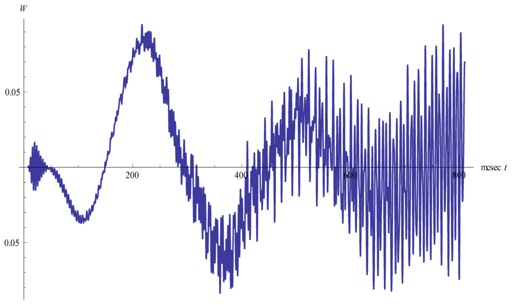
Figure 1. Density oscillations for the case of no helicity.

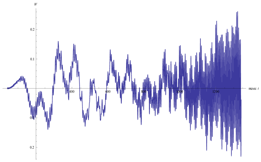
Figure 2. Density oscillations for the case of present helicity.

As seen, density oscillations arise. High-frequency oscillations (f = 266 kHz) are modulated by a low-frequency signal (f = 3.3 kHz). First of all, the amplitude of the oscillations increases, then decreases. Later on, the amplitude of the low-frequency oscillations grows and the picture becomes a chaotic one. Figure 3 and Figure 4 show the density oscillations as they decay.

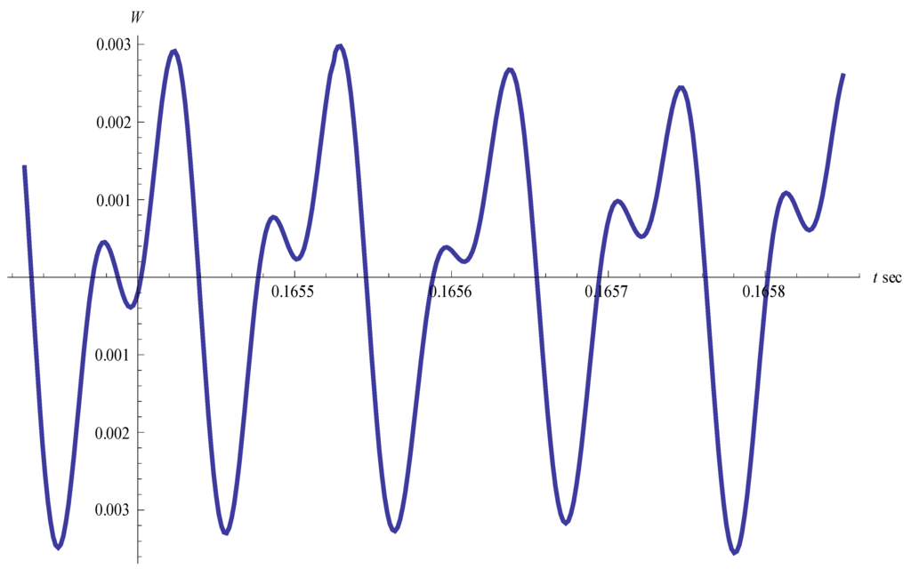
Figure 3. Density oscillations at the final stage of the process (no helicity).

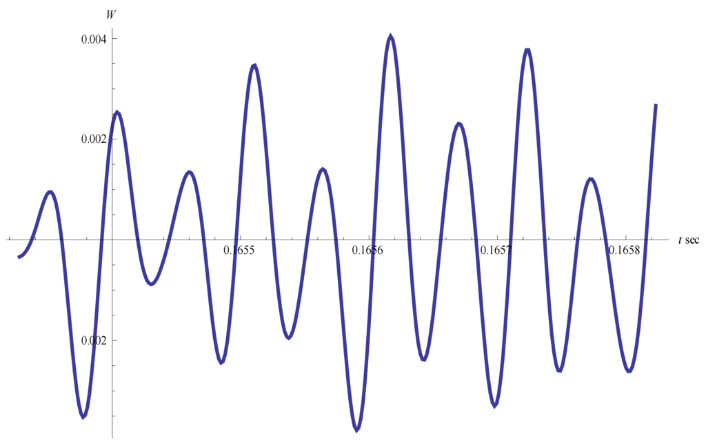
Figure 4. Density oscillations at the final stage of the process (helicity is present).

Figure 5 and Figure 6 represent the density oscillations inside the initial domain of the toroid.

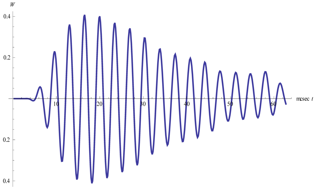
Figure 5. Density oscillations inside the initial vortex ring (no helicity).

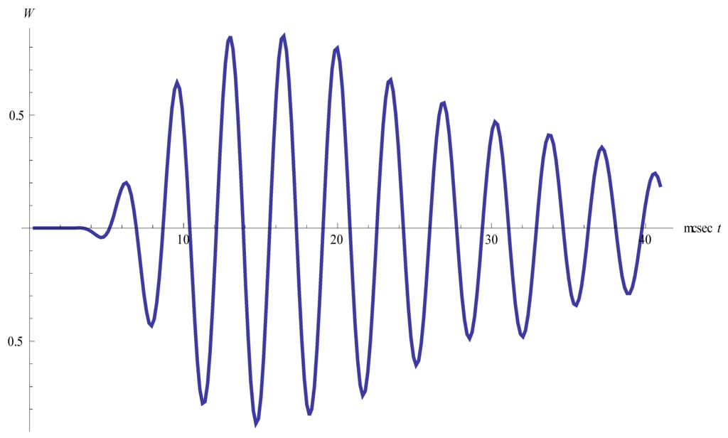
Figure 6. Density oscillations inside the initial vortex ring (helicity is present).

One can see that the high-frequency component of the oscillations does not depend on helicity. The presence of helicity has an effect only on the amplitude of the oscillations increasing it. The value of high frequency remains constant during the whole process excluding the final stage of the process (see Figure 3 and Figure 4). The value of high frequency corresponds satisfactorily to the experimental data in [14]. In these experiments an unstable vortex ring appeared behind a shock wave reflected from a concave body. The radius of the ring was equal to 0.1 cm, the frequency of oscillations was 170–220 kHz.

4. Conclusions

A new method is set forth which allows us to investigate the frequency of acoustic radiations by 3D vortex rings. As shown, helicity has no effect on the frequency of the high-frequency component. The results may be of interest for aeroacoustics.

References

- Howe, M.S. Theory of Vortex Sound; Cambridge University Press: Cambridge, UK, 2003. [Google Scholar]
- Lighthill, M.J. On sound generated aerodynamically. Proc. Roy. Soc. A 1952, 211, 564–587. [Google Scholar] [CrossRef]
- Powell, A. Theory of vortex sound. J. Acoust. Soc. Am. 1964, 36, 177–195. [Google Scholar] [CrossRef]
- Kopiev, V.F.; Chernyshev, S.A. Vortex ring eigen oscillations as a source of sound. J. Fluid Mech. 1997, 341, 19–57. [Google Scholar] [CrossRef]
- Verzicco, R.; Iafrati, A.; Riccardi, G.; Fatica, M. Analysis of the sound generated by the pairing of two axisymmetric corotating vortex rings. J. Sound Vibr. 1997, 200, 347–358. [Google Scholar] [CrossRef]
- Inoue, O. Sound generation by the leapfrogging between two coaxial vortex rings. Phys. Fluids 2002, 14, 3361–3364. [Google Scholar] [CrossRef]
- Maxworthy, T.J. Turbulent vortex rings. J. Fluid Mech. 1974, 64, 227–240. [Google Scholar] [CrossRef]
- Maxworthy, T.J. Some experimental studies of vortex rings. J. Fluid Mech. 1977, 81, 465–495. [Google Scholar] [CrossRef]
- Liu, C.; Yan, Y.; Lu, P. Physics of turbulent generation and sustenance in a boundary layer. Comput. Fluids 2014, 102, 353–384. [Google Scholar] [CrossRef]
- Yan, Y.; Chen, C.; Fu, H.; Liu, C. DNS study on Λ-vortex and vortex ring formation in flow transition at Mach number 0.5. J. Turbul. 2014, 15, 1–21. [Google Scholar] [CrossRef]
- Morton, T.S. The velocity field within a ring with a large elliptic cross-section. J. Fluid Mech. 2004, 503, 247–271. [Google Scholar] [CrossRef]
- Truesdell, C. Precise theory of the absorption and dispersion of forced plane infinitesimal waves according to the Navier–Stokes equations. J. Ration. Mech. Anal. 1953, 2, 643–721. [Google Scholar] [CrossRef]
- Korobov, N.M. Theoretical and Numerical Methods in Approximate Analysis; Moscow State University: Moscow, Russian, 1963. [Google Scholar]
- Shugaev, F.V.; Shtemenko, L.S. Propagation and Reflection of Shock Waves; World Scientific Publishing: Singapore; Hackensack, NJ, USA; London, UK; Hong Kong, China, 1998. [Google Scholar]
© 2015 by the authors; licensee MDPI, Basel, Switzerland. This article is an open access article distributed under the terms and conditions of the Creative Commons Attribution license (http://creativecommons.org/licenses/by/4.0/).