Article

East–West GEO Satellite Station-Keeping with Degraded Thruster Response

Aerospace Engineering, Texas A&M University, College Station, TX 77843, USA
*
Author to whom correspondence should be addressed.
Aerospace 2015, 2(4), 581-601; https://doi.org/10.3390/aerospace2040581
Submission received: 6 April 2015 / Revised: 21 August 2015 / Accepted: 11 September 2015 / Published: 29 September 2015
(This article belongs to the Special Issue Feature Papers in Aerospace)

Abstract

:
The higher harmonic terms of Earth’s gravitational potential slowly modify the nominal longitude of geostationary Earth orbit (GEO) satellites, while the third-body presence (Moon and Sun) mainly affects their latitude. For this reason, GEO satellites periodically need to perform station-keeping maneuvers, namely, east–west and north–south maneuvers to compensate for longitudinal and latitudinal variations, respectively. During the operational lifetime of GEO satellites, the thrusters’ response when commanded to perform these maneuvers slowly departs from the original nominal impulsive behavior. This paper addresses the practical problem of how to perform reliable east–west station-keeping maneuvers when thruster response is degraded. The need for contingency intervention from ground-based satellite operators is reduced by breaking apart the scheduled automatic station-keeping maneuvers into smaller maneuvers. Orbital alignment and attitude are tracked on-board during and in between sub-maneuvers, and any off nominal variations are corrected for with subsequent maneuvers. These corrections are particularly important near the end of the lifetime of GEO satellites, where thruster response is farthest from nominal performance.

Graphical Abstract

1. Introduction

Over time, a geostationary Earth orbit (GEO) satellite will drift both in longitude and latitude because of the presence of various perturbations. These perturbations mainly are the gravitational forces caused by Earth longitudinal mass variations, the gravitational presence of the Moon and Sun and the solar radiation pressure [1,2]. The persistent gravitational perturbations create two stable and two unstable equilibrium points along the GEO belt at 75.91 east and 102.92 west and 164.1 east and 10.62 west, respectively. Because of these perturbations, the nominal location of a GEO satellite, in the Earth-centered Earth-fixed (ECEF) reference frame, changes as the satellites drift away from the unstable equilibrium points towards the stable equilibrium points. To maintain the GEO satellite within its specified longitudinal and latitudinal bounds, periodic corrective impulses must be applied (satellite station keeping), with satellites nearer the unstable equilibrium points requiring more vigorous station keeping. Current methods of station keeping rely on a single maneuver, which corrects the longitude and longitude drift rate once the satellite drifts near the edges of the acceptable longitudinal range, as shown in Figure 1. The effect of the maneuver is illustrated in Figure 2.
Figure 1. East–west (E–W) station-keeping deadband of a GEO satellite.
Aerospace 02 00581 g001
Figure 2. Phase trajectory of the GEO E–W station-keeping using a stable thruster under λ ¨ < 0 .
Aerospace 02 00581 g002
However, station-keeping maneuvers will provide unreliable or unexpected results if the thruster performance changes from its expected nominal behavior. This leads to an imperfect correction and potentially to extreme longitudinal drift of the satellite, causing loss in communications quality. It is especially dangerous if the satellite operators are not aware of the degraded thruster response and have not accounted for the imperfect correction in their control scheme. The degradation of thrusters’ performance (electrical or chemical) is especially noticeable at the end of the GEO lifetime. Furthermore, thruster mounting deviations, installation bias, shock shift, thermal deformation, etc., may all lead to non-nominal and/or asymmetric thrusts.
In these cases, the east–west (E–W) maneuver strategy to adjust the mean longitude must be re-formulated, and a new model is needed to still provide efficient control. The design of this model is the main purpose of this paper. In other words, this paper provides an answer to the following question: “How can a GEO satellite still performing E–W maneuvers using unreliable and degraded thrusters?”. To solve this problem, the following issues must be resolved:
  • Modeling the effect of degraded thruster response on longitudinal station keeping;
  • The new control approach is more complex and, therefore, is at higher risk of performing the wrong maneuvers;
  • The number of satellite operations increases, as well as extra work is required from ground operators;
  • In some cases, the thrusters generate unexpected orbital deviations; in these cases, the on-board program must be able to eventually interrupt and alter the control strategy;
  • Orbital elements and satellite dynamics must be tracked during and between maneuvers in order to ensure correct station keeping.
This paper investigates a potential solution to this problem by analyzing the variation of angular momentum in the satellite’s momentum wheels to estimate the change of orbital elements, such as the semi-major axis and eccentricity. Once these variations are known, a correcting maneuver loop is constructed and executed. A concise work-flow, which follows this methodology for performing reliable E–W station keeping under degraded thrusters, is presented at the end of this paper.

2. Nominal East–West GEO Satellite Drift

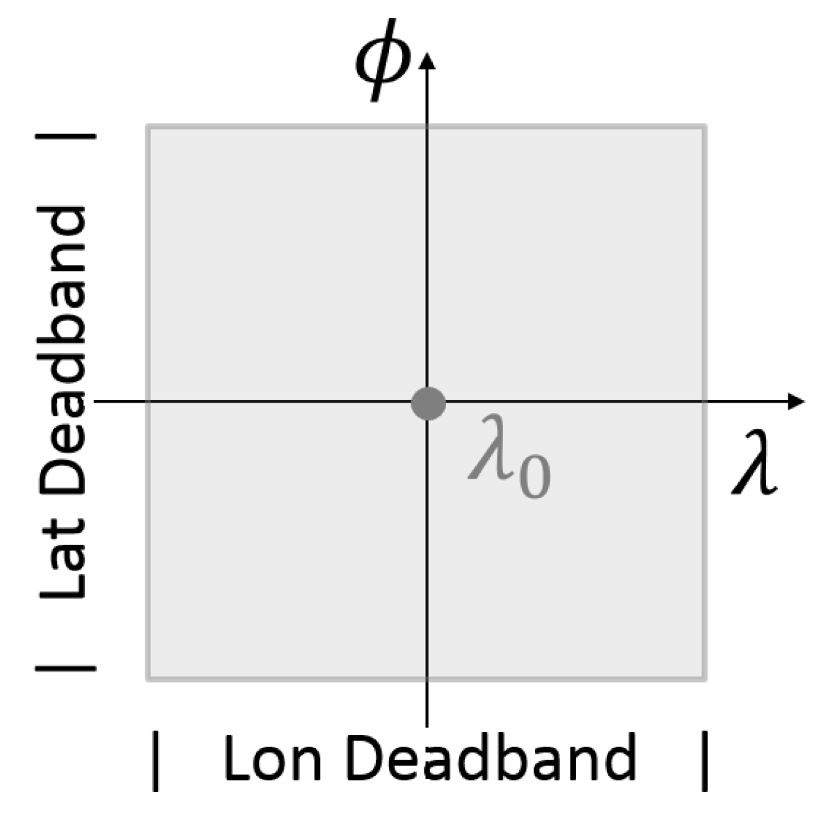
2.1. Longitudinal “Deadband”

Figure 1 shows the latitudinal and longitudinal range (deadband) within which a GEO satellite is supposed to remain during its operative time. This box is usually small, because ground users do not want to re-point their communications antenna and because the GEO belt is becoming very crowded in terms of frequency allocation [3]. By going outside that deadband, the communications quality degrades (or even gets lost), and the communications may interfere with the communications of neighbor GEO satellites. However, the asymmetric distribution of the Earth’s gravitational field creates persistent perturbation forces pushing the GEO satellite outside the assigned deadband.
The purpose of GEO station keeping is to keep the GEO satellite longitude and latitude point inside the rectangular “deadband” box [4]. Let Δ λ D B be the E–W maximum allowed longitudinal excursion. This means that the satellite longitude is constrained to be in the longitude range λ [ λ 0 - Δ λ D B , λ 0 + Δ λ D B ] , where λ 0 is the assigned GEO satellite’s nominal longitude. Depending on the λ 0 value and on the communications constraints, the E–W deadband ranges from a fraction to a few degrees.

2.2. Lagrange’s Equations of Drift Rate

The main perturbing forces acting on GEO satellites are: (1) the “third body” (Moon and Sun gravitational presence); (2) the solar pressure (GEO satellites usually have large solar arrays); and (3) the tangential forces generated by the non-axially symmetric distribution of the Earth’s mass. While the third body and the solar pressure are periodic perturbations, the higher harmonic terms of the Earth gravitational potential have a persistent perturbing effect on the GEO satellites, because their nominal positions should be, in theory, fixed in the ECEF reference frame [5]. The orbital parameters that mainly change are: inclination (i), eccentricity (e) and semi-major axis (a). Variation of e and a cause variations of the geographic longitude [6].
The perturbing potential generated by the non-axially symmetric distribution of the Earth’s mass can be described by a limited set of coefficients describing the Earth gravitational potential:
R = μ r { - 1 2 J 2 R e r 2 + 3 J 22 R e r 2 cos 2 ( λ - λ 22 ) + - 3 2 J 31 R e r 3 cos ( λ - λ 31 ) + 15 J 33 R e r 3 cos 3 ( λ - λ 33 ) + + 3 8 J 4 R e r 4 }
where R e is the mean equatorial radius of the Earth, r is the geocentric distance of the satellite, μ is the Earth’s central gravity constant and J 2 , J 22 , J 31 , J 33 and J 4 are the zonal harmonic coefficients of the Earth’s gravity potential field.
The vector { a , λ } , made by the semi-major axis and the mean longitude, is used to describe the drift of the GEO satellite. In particular, the mean longitude can be expressed as:
λ = ω + Ω + M - θ ( t )
where ω is the argument of perigee, Ω is the right ascension of the ascending node, M is the mean anomaly and θ ( t ) is the true anomaly.
The rate of change of the drift vector can be described by the Lagrange planetary equations, which can be written as (with eccentricity and inclination expanded to the first order):
d a d t = 2 n a R λ = - 2 3 a c n c λ ¨ d λ d t = ( n - ω e ) - 2 n a R a = - 3 2 n c a c ( a - a c )
where a is the perturbed semi-major axis (affected by the harmonic terms of the Earth potential), n c = 2 π / 86 , 164 . 09 is the Earth’s rotation rate and λ ¨ is the longitudinal acceleration:
λ ¨ = - 3 n c 2 { - 6 J 22 R e a c 2 sin 2 λ - λ 22 + 3 2 J 31 R e a c 3 sin λ - λ 31 - 45 J 33 R e a c 3 sin 3 λ - λ 33 }
Consider the equations of the longitudinal dynamics with some specific initial values:
d d t λ = d λ d t = λ ˙ λ | t = t 0 = λ 0 d d t d λ d t = d d t λ ˙ = λ ¨ n = const d λ d t | t = t 0 = λ ˙ 0
Under the practical assumption that the longitude variation over one cycle is small (the typical longitudinal range, or deadband, for the E–W cycle is usually lower than ± 0 . 5 ), it is reasonable to consider as constant the longitudinal acceleration during a cycle. The solution for the longitudinal variation under constant acceleration is then obtained by integrating Equation (5):
λ = λ 0 + λ ˙ 0 t + 1 2 λ ¨ n t 2 λ ˙ = λ ˙ 0 + λ ¨ n t
where the subscript “0” indicates values evaluated at time t = 0 . Equation (6) describes a parabolic motion in the phase space, as seen in Figure 2.
The initial drift velocity, λ ˙ 0 , is an initial condition, and the required bound, Δ λ D B , is the assigned deadband requirement in which the satellite must remain. The drift time between two consecutive E–W maneuvers,
T = 4 Δ λ | λ ¨ | ,
and Δ V , the impulse provided at each cycle, are computed as specified in [7] and Equation (8).
Over the drift time, T, the GEO satellite changes the drift rate from λ ˙ 0 to - λ ˙ 0 , as seen in Figure 2. The associated impulse, Δ V , for each maneuver is:
Δ V = 11 . 32 Δ λ | λ ¨ |

2.3. Nominal Single E–W Maneuver

Figure 2 shows the nominal E–W station-keeping maneuver of a GEO satellite, subject to the constant longitude drift acceleration (here assumed negative, λ ¨ < 0 ), with assigned nominal longitude λ 0 . Every time the longitude reaches the value λ 0 - Δ λ D B , the E–W thruster provides an impulse changing the longitude velocity from - λ ˙ to + λ ˙ . This burn brings the GEO satellite to reach the other edge of his E–W deadband, λ 0 + Δ λ D B , with longitude velocity λ ¨ = 0 . This cycle is then repeated, and the GEO satellite is kept within the deadband limits, λ 0 ± Δ λ D B . The perturbing longitudinal acceleration λ ¨ is known from Equation (4).
Figure 3. Simple control scheme near the stable node with λ ¨ < 0 .
Aerospace 02 00581 g003
Figure 4. Simple control scheme using incorrect thrust near the unstable node with λ ¨ < 0 .
Aerospace 02 00581 g004
Control schemes require different levels of thrust depending on the nominal latitude of the satellite. More thrust is required to maintain latitude within the deadband for satellites near the unstable longitude nodes. Figure 3 demonstrates how a nominal repeated control scheme would work near the stable node. Figure 4 demonstrates a control scheme that uses the same thrust applied near the unstable node. The satellite latitude still remains within the deadband; however, much more frequent thrusting is required. A degraded thruster might respond in a similar fashion, leading to the more frequent need for emergency thrusts to keep the satellite within the required deadband. Settling near one edge of the deadband might also reduce the utility of the satellite or decrease the communication signal strength. Obviously, if the degraded thruster response is unpredictable, it is possible to over-correct, sending the satellite out beyond the permissible deadband.

2.4. Station-Keeping Strategy Using a Degraded E–W Thruster

The proposed station-keeping strategy consists of a cyclic procedure using the following steps:
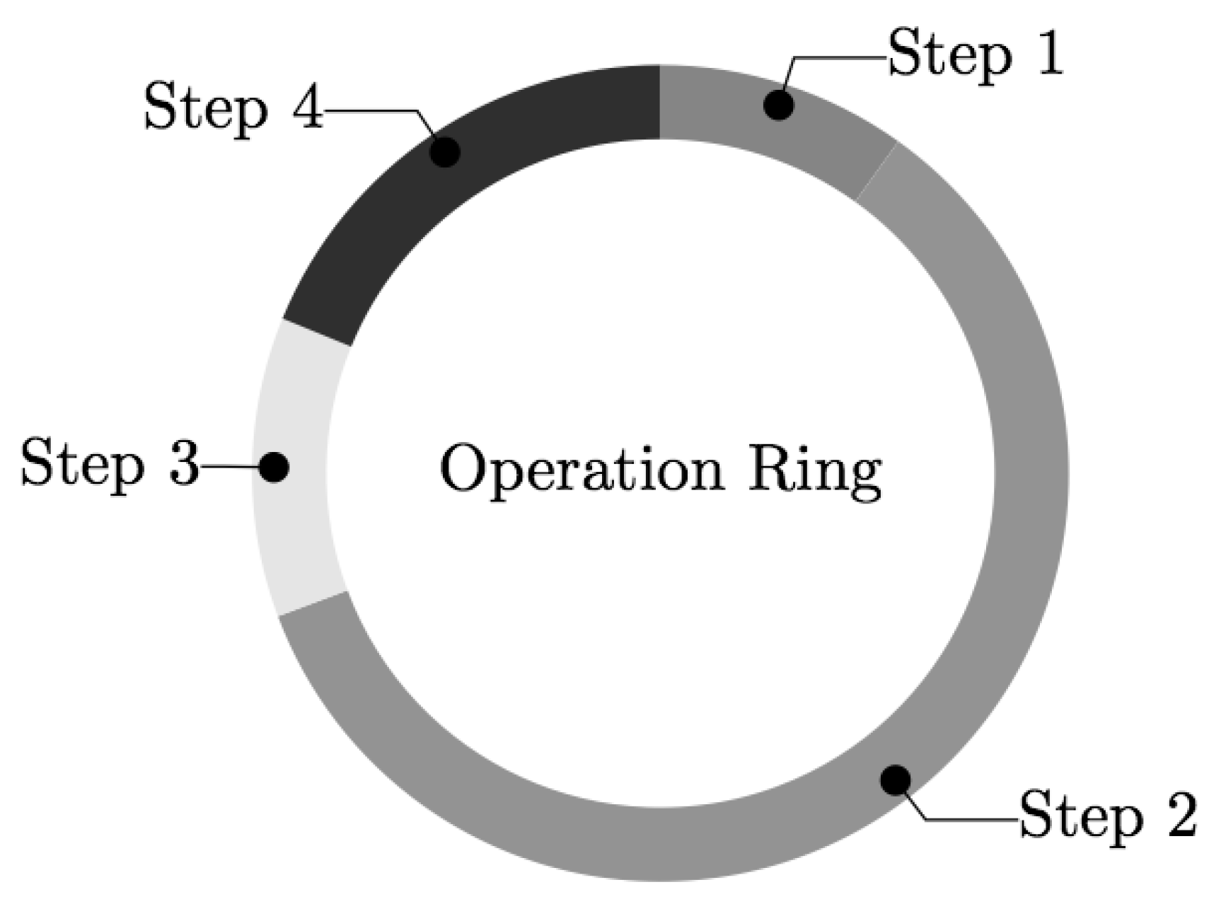
  • Step 1: Station-keeping. In this phase, the on-board control thrusters execute the orbital maneuvers to keep the GEO satellite in its assigned deadband. These maneuvers can be evaluated on-board or at ground stations.
  • Step 2: Longitude drift. In this phase, the GEO satellite, subject to the Earth’s tesseral harmonics, drifts in its longitude toward east or west, depending on where the closest stable longitude point sits.
  • Step 3: Orbit measurements. In this phase, all of the input data for the orbit determination algorithms are measured. These measurements can be obtained by ground-based observers, telescopes or radars. These data usually consist of time, azimuth, elevation, range and/or range rate. Usually, to obtain enough accuracy for orbit determination, measurements should be taken over at least one full day.
  • Step 4: Orbit determination. Specific orbit determination algorithms are used to estimate the orbit. These algorithms can be run on the ground or simplified versions can be run on-board. The difference between the expected orbit (before the impulse) and the measured orbit (after the orbit determination phase) constitutes the error. The analysis of this error then dictates the next station-keeping strategy as more reliable knowledge is obtained on the effectiveness of the thrusters.
The above station-keeping strategy is simplified in the cyclic activities shown in Figure 5.
Figure 5. Ideal cycle of the E–W station-keeping operation.
Aerospace 02 00581 g005
The cycle described above is repeated until the velocity reaches the nominal curve in the phase plane. This may require several cycles. Just to show an example, Figure 6 shows the resulting variations of velocity ( Δ λ ˙ ) obtained by five cycles to reach the curve in the phase plane.
Figure 6. Example of five loops of the operation ring of E–W station-keeping.
Aerospace 02 00581 g006
The nominal single E–W maneuver is split here into five smaller E–W maneuvers. Between any two consecutive maneuvers, there will be a short drifting time and then a period of time dedicated to the orbit measurements to perform the orbit determination.

2.5. Control Equations of the E–W Maneuver

The equation of the dynamics of a GEO satellites can be linearized by introducing the variation in geographical longitude with respect to the nominal value [7]. Under the assumption that the impulse is planar ( Δ V r = 0 , Δ V n = 0 and Δ V t 0 ), the linearized equations of motion describing E–W orbit maneuvers yield the following equations ruling the orbital parameter variation:
Δ r = a s 2 3 Δ λ ˙ + Δ e x cos b + Δ e y sin b Δ λ = Δ λ D B + Δ λ ˙ b - 0 + 2 Δ e x sin b - Δ e y cos b Δ V r = V s Δ e x sin b - Δ e y cos b = 0 Δ V t = V s Δ λ ˙ + 2 Δ e x cos b + 2 Δ e y sin b
where a s = 42 , 168 . 74 km is the semi-major axis of the geosynchronous orbit, b is the sidereal angle to the GEO satellite position, V s = 3 . 0747 km/s is the orbital velocity of the GEO satellite and Δ e x and Δ e y are the first and second components of the eccentricity vector.
If the impulse is tangential and instantaneous, then Δ r = 0 and Δ λ = 0 . Therefore, Equation (9) can be rewritten in matrix form:
2 / 3 0 cos b cos b b - 0 1 2 sin b - 2 cos b 0 0 sin b - cos b V s 0 2 V s cos b 2 V s sin b Δ λ ˙ Δ λ D B Δ e x Δ e y = 0 0 0 Δ V t
whose solution is:
Δ λ ˙ = - 3 Δ V t V s τ [ deg/day ] Δ λ D B = 3 Δ V t V s b - 0 [ deg ] Δ e x = 2 Δ V t V s cos b Δ e y = 2 Δ V t V s sin b
where τ = 360 . 985647 deg/day is the Earth’s rotation angle per mean sidereal day and 0 is the sidereal angle at the thrust firing time t b .

3. Degraded Thruster Response

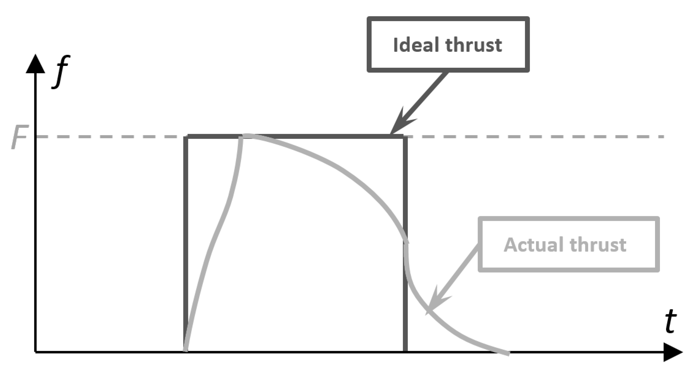
3.1. Comparison of the Time-Domain Output of the Thruster Pulse

The thrust performing the E–W maneuver usually fires for a short time (about a minute) as compared to the GEO orbital period. For this reason, this maneuver is considered impulsive. Unfortunately, an impulsive thrust (constant thrust during the firing time) is an idealization that approximates the thrust behavior only at the beginning of its lifetime (see Figure 7).
Thruster performance degrades over time, especially near the end of the mission lifetime (see Figure 8).
Figure 7. Thruster response at the beginning of its lifetime.
Aerospace 02 00581 g007
Figure 8. Thruster response at the end of its lifetime.
Aerospace 02 00581 g008
In Figure 7 and Figure 8, the dark curves indicate the ideal thruster responses (or the electrical “ON” command), while the lighter curves describe the actual thruster responses.

3.2. E–W Maneuver with Degraded Thruster Response

The complexity of system Equation (10) is due to the existence of the parasitic unstable thrust response. This effect can be removed from the equations and instead treated as mere disturbance, which must be considered during the analysis stage of the maneuver operation. This analysis would be done in between maneuvers, such as the ones shown in Figure 6.

4. Attitude Dynamics of the Momentum-Biased GEO Satellites

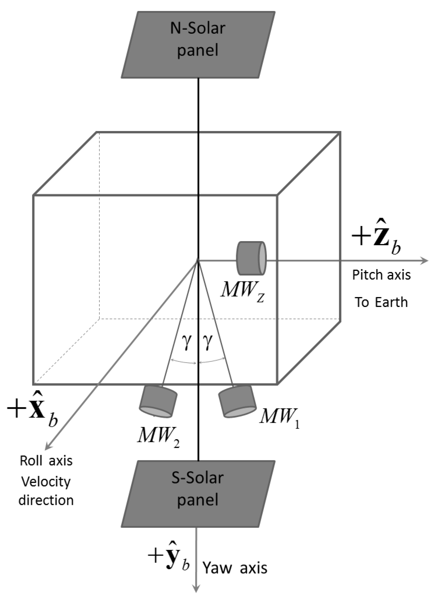
4.1. Momentum-Biased Wheel Configuration

Let us consider a typical momentum-biased GEO satellite, as shown in Figure 9, where MW indicates the momentum wheels. The satellite body frame is indicated by the three orthogonal axes x ^ b , y ^ b and z ^ b . The pitch axis, z ^ b , is kept pointing to nadir (to Earth) and is the axis along which the communication antenna is aligned. The roll axis, x ^ b , is the orbit tangential axis, which is aligned with the orbital velocity vector, and the yaw axis, y ^ b , which is the axis orthogonal to the orbital plane, is aligned with the orbital angular momentum. The typical attitude control of this GEO satellite involves three momentum wheels. Two of them, which are the nominal control wheels, are mounted in a “V” configuration with the two spinning axes on the y ^ b z ^ b plane and displaced form the y ^ b axis by an angle γ.
Figure 9. Momentum-biased wheel configuration.
Aerospace 02 00581 g009
In this type of satellite, a constant momentum bias, h w y 0 , is applied along the y ^ b axis to keep the GEO spin rate (around the y ^ b axis) equal to the orbit mean motion. The two momentum wheels in the “V” configuration provide E–W inertial angular stability and are dedicated to controlling yaw angle. A third smaller momentum wheel, M W Z , is mounted with its spin axis aligned along the z ^ b body axis. If one of the primary wheels ( M W 1 or M W 2 ) fails, then this backup wheel, which is nominally kept inactive, can now be used to provide the momentum bias in place of the failed wheel.
The two primary wheels, M W 1 and M W 2 , provide a total momentum bias of H w = 2 H 1 cos γ aligned along the y ^ b axis. The torques, T y c and T z c , provided by these wheels are related to the angular momentum rate components, H ˙ 1 and H ˙ 2 , by the equation:
T y c T z c = cos γ cos γ sin γ - sin γ H ˙ 1 H ˙ 2
This means that, to obtain the torque commands (as required by the attitude control law), the wheels should provide the angular momentum rates:
H ˙ 1 H ˙ 2 = 1 2 1 / cos γ 1 / sin γ 1 / cos γ - 1 / sin γ T y c T z d
The angular momentum of the wheels is related to the wheels’ moment of inertia, I w x , I w y and I w z , and to the wheels’ angular velocities, ω w x , ω w y and ω w z , by:
h w x = I w x ω w x , h w y = I w y ω w x + h w y 0 , and h w z = I w z ω w z .
Thus, we have:
h w y h w z = cos γ cos γ sin γ - sin γ H 1 H 2 and h ˙ w y h ˙ w z = cos γ cos γ sin γ - sin γ H ˙ 1 H ˙ 2
The angular momentum vector in body coordinates is:
h = h x h y + h w y h z + h w z = h x h y + ( H 1 + H 2 ) cos γ h z + ( H 1 - H 2 ) sin γ
If the wheels’ momentum biases are equal, H 1 ( 0 ) = H 2 ( 0 ) = H ( 0 ) , we can write:
H 1 + H 2 = 2 H ( 0 ) + T y c cos γ d t
and:
H 1 - H 2 = T z c sin γ d t
Euler’s moment equation, M = h ˙ I = h ˙ + ω × h , can be written with h w x 0 , since there is no momentum wheel projection on the x ^ b axis. In this equation, subscript “I” indicates the derivative evaluated in the inertial frame, while h ˙ is the derivative of the angular momentum vector, h , in the body frame. This yields the equations used to simulate the body attitude dynamics:
T x c + T x d = h ˙ x + ω y ω z ( I z - I y ) + ω y ( H 1 - H 2 ) sin γ - ω z ( H 1 + H 2 ) cos γ T y c + T y d = h ˙ y + ω x ω z ( I x - I z ) + ( H ˙ 1 + H ˙ 2 ) cos γ - ω x ( H 1 - H 2 ) sin γ T z c + T z d = h ˙ z + ω x ω y ( I y - I x ) + ( H ˙ 1 - H ˙ 2 ) sin γ + ω x ( H 1 + H 2 ) cos γ
Consider that the products of inertia are zero and h w x = h ˙ w x = 0 . Under these assumptions, the linearized attitude dynamics equations from [12] are derived:
T x c + T x d = I x ψ ¨ + 4 ω 0 2 ( I y - I z ) ϕ + ω 0 ( I y - I z - I x ) ψ ˙ - ω 0 ( H 1 - H 2 ) sin γ T y c + T y d = I y θ ¨ + 3 ω 0 2 ( I x - I z ) θ + ( H ˙ 1 + H ˙ 2 ) cos γ T z c + T z d = I z ψ ¨ + ω 0 ( I z + I x - I y ) ϕ ˙ + ω 0 2 ( I y - I x ) ψ + ( H ˙ 1 - H ˙ 2 ) sin γ
In these equations, the angular velocity vector, ω, is provided by its components, ω x , ω y and ω z , along the body axes, and ϕ, θ and ψ are the Euler angles defined about the coordinate axes x ^ b , y ^ b and z ^ b , respectively.

4.2. Orbital Element Estimation Based on the Angular Momentum Wheel Variations

For an elliptical orbit, the orbital energy conservation equation (vis-vivaequation) is written as:
v 2 2 - μ r = - μ 2 a where r = a ( 1 - e cos E ) .
Using this energy equation, it is easy to derive the relationship between applied velocity variation, Δ v , and semi-major axis variation:
Δ a = 2 a 2 μ 2 r - 1 a Δ v
For a geostationary satellite, we have r a a s = 42 , 164 . 2 km and ω s ω e = 7 . 2921158479 · 10 - 5 rad/s. Furthermore, using Δ V T = Δ v for the impulsive velocity variation, Equation (22) can be rewritten as:
Δ a = 2 ω e Δ V T
Let J x , J y and J z , be the three principal moments of inertia of the satellite body. Ω x , Ω y , Ω z are the angular velocities defined about the body axes. Considering two equally-balanced momentum wheels with angular momentum H w , the net effect is:
J x = J z = 0 , J y = J and Ω y = Ω , Ω x = Ω z = 0 .
The momentum bias of the wheel about the y ^ b axis is denoted by h w , with its radius R w , so that:
h w = J Ω = J R w v w
Next, we differentiate Equation (25); this yields:
Δ h w = J Δ Ω = J R w Δ v w
From which, together with R w = h 0 J v 0 , we find that:
Δ h w Δ v w = h 0 v 0
where h 0 denotes the nominal angular momentum of an MW with respect to its nominal speed v 0 .
For practical reasons, the total torque T y , acting on the y ^ -axis in the body frame, is broken down into two principal parts: T y c , the control moments to be used for controlling the yaw attitude motion of the satellite, and T y d , the moments due to different environmental disturbances. The total torque vector is thus T y = T y c + T y d . According to Equation (20), the MW’s momentum change (e.g., h ˙ w ) will produce an equal and opposite angular torque on the body about its y ^ b body axis, T y c = - h ˙ w . If Ω ˙ is the angular acceleration of the y ^ b axis wheel, then h ˙ w = J Ω ˙ is the negative of the angular moment that the y ^ b wheel exerts on the satellite about its y ^ b axis.
Assuming that the net torque on the satellite is zero, we have:
T y c + T y d = 0
This means that, if a torque is induced by a thrust vector on the body about the y ^ b axis, a torque in the opposite direction must be produced by the rotor of the electrical motor. Thus, T y c = - T y d . In the momentum differential expression, we get:
Δ h w = T y d d t = T y d Δ t = l x f z Δ t
The term Δ h w is the angular moment that the wheel exerts on the satellite along the y ^ b body axes. In Figure 10, the thrust vector f along the z ^ b body axis is denoted as f z i ^ , which is perpendicular to the corresponding equivalent torque arm l x j ^ , where l x f z Δ t is the torque impulse generated by thrust component f z j ^ .
Figure 10. Thruster output of longitudinal station-keeping (westward) defined in the body frame.
Aerospace 02 00581 g010
Let us denote m the entire mass of the satellite. Assuming that β is the satellite yaw angle and based on the theorem of momentum, we get:
m Δ V T = f x Δ t where f x = f z tan β
Moreover, substituting Equations (27) and (30) into (29), we derive:
h 0 v 0 Δ v w = l x tan β m Δ V T
from which it follows that:
Δ V T = h 0 tan β v 0 m l x Δ v w κ Δ v w
Knowing the tangential velocity change, we can calculate the change of corresponding orbital elements from Equations (11) and (23); it is easily found that:
Δ a = 2 ω e Δ V T = 2 κ ω e Δ v w K a Δ v w Δ λ ˙ = - 3 τ V s Δ V T = - 3 τ κ V s Δ v w K D Δ v w | Δ e | = 2 V s Δ V T = 2 κ V s Δ v w K e Δ v w
with K a , K d , K e and κ defined as follows:
κ h 0 tan β v 0 m l x K a 2 κ ω e K D - 3 τ κ V s K e 2 κ V s
Substituting all known m, l x , β, h 0 , ω e , v 0 and V s into Equation (34) yields the constants K a , K D , K e and κ. Equation (33) is the desired result, because it gives the expression of the variation in orbital elements with respect to the variation in MW velocity.

5. Simulation Case

The following steps describe the application of the theoretical models described so far.
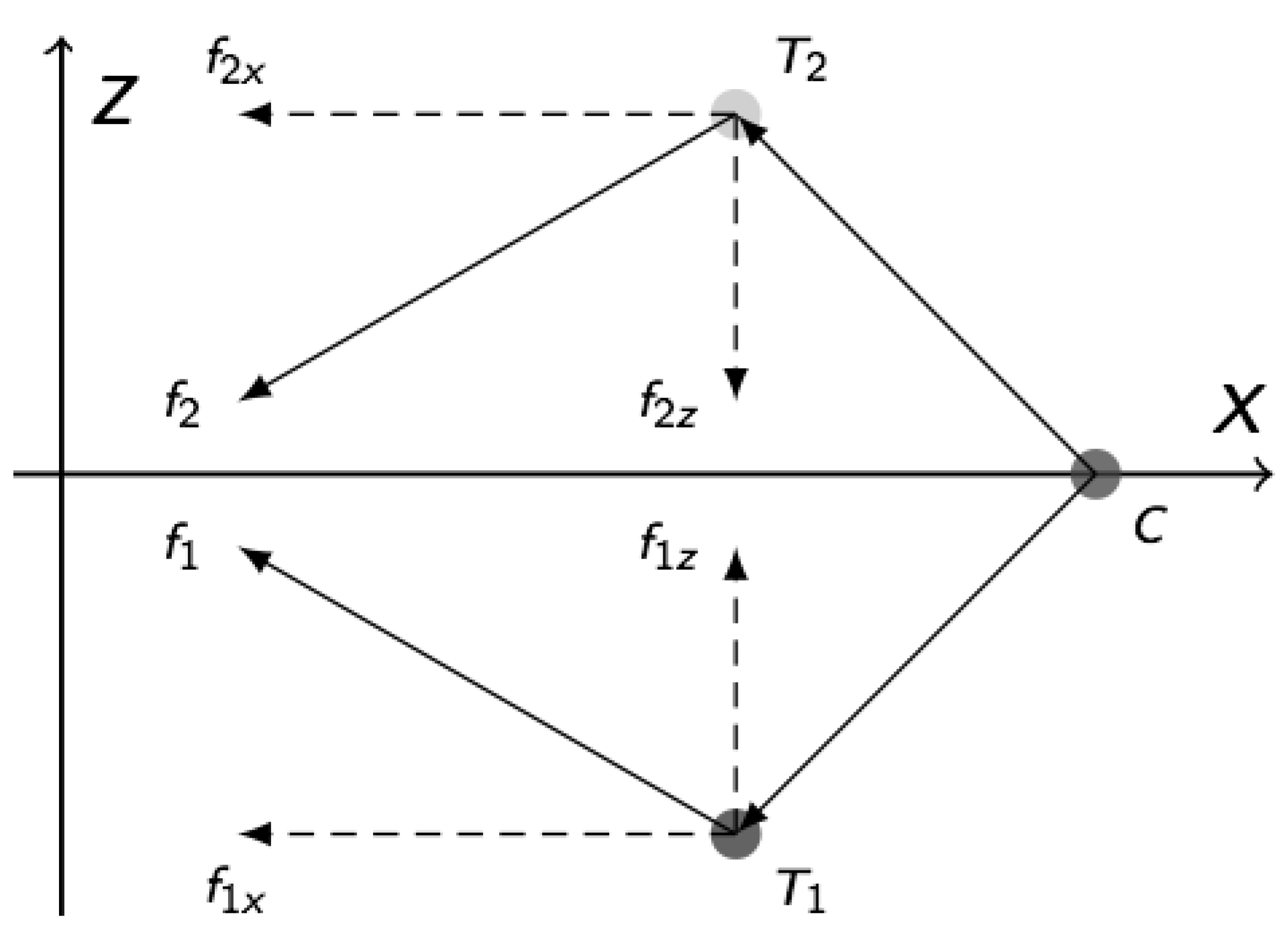
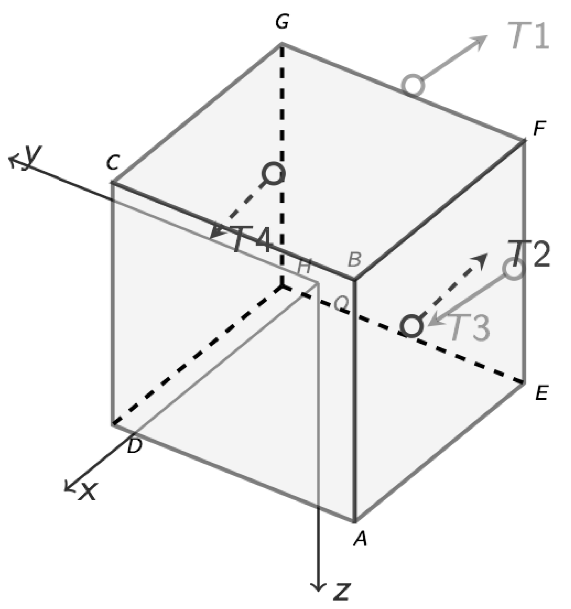
  • Scenario and inputs: Let us adopt the following values for the purposes of simulation: mean east longitude = 80.0 E, satellite mass = 2400 kg, cross-sectional area = 10 m 2 and reflectivity constant = 1.85. The momentum biases in the wheels, H 1 and H 2 , have both been determined to be 10 N·m·s; the installation inclination angle γ = 25 is a reasonable choice. To provide momentum bias attitude control, the momentum wheels are spun with an angular velocity of 1000 rpm, which is inside the permitted bounds for the MWs. A reaction bipropellant low-thrust system consists of two 10 N thruster pairs. Illustrated in Figure 11, the thrusters are arranged so that they provide the necessary torques for attitude control about the three body axes, as well as the necessary thrust for station keeping. Thruster pairs of T 1 and T 2 , T 3 and T 4 are used for E–W (longitude) station keeping and also for eccentricity corrections. Thrusters T 1 and T 2 provide the positive and the negative yaw control torques respectively about the y ^ b axis; likewise, thrusters T 3 and T 4 yield the positive and the negative torques individually about the z ^ b axis.
    Figure 11. Possible thruster setup for a GEO satellite.
    Figure 11. Possible thruster setup for a GEO satellite.
    Aerospace 02 00581 g011
  • Dynamics: From Equation (4), we can obtain the longitude drift acceleration, λ ¨ = - 3 . 628 · 10 - 4 deg/day 2 . Then, we calculate the needed Δ V from Equation (8) for the entire sequence of corrections. This is useful for giving a rough estimate for how much fuel will be spent during the maneuvering sequence. Substituting all constants into Equation (34) and simplifying, we obtain Δ a 1 = 1.44927 · 10 - 4 Δ v 1 w km, Δ a 2 = 1.492537 · 10 - 4 Δ v 2 w km. We also get the desired correction in longitude drift rate Δ λ ˙ . After each thruster firing, Δ v 1 w and Δ v 2 w will be measured, and Δ a 1 and Δ a 2 will be calculated and used to determine how much more correction is needed.
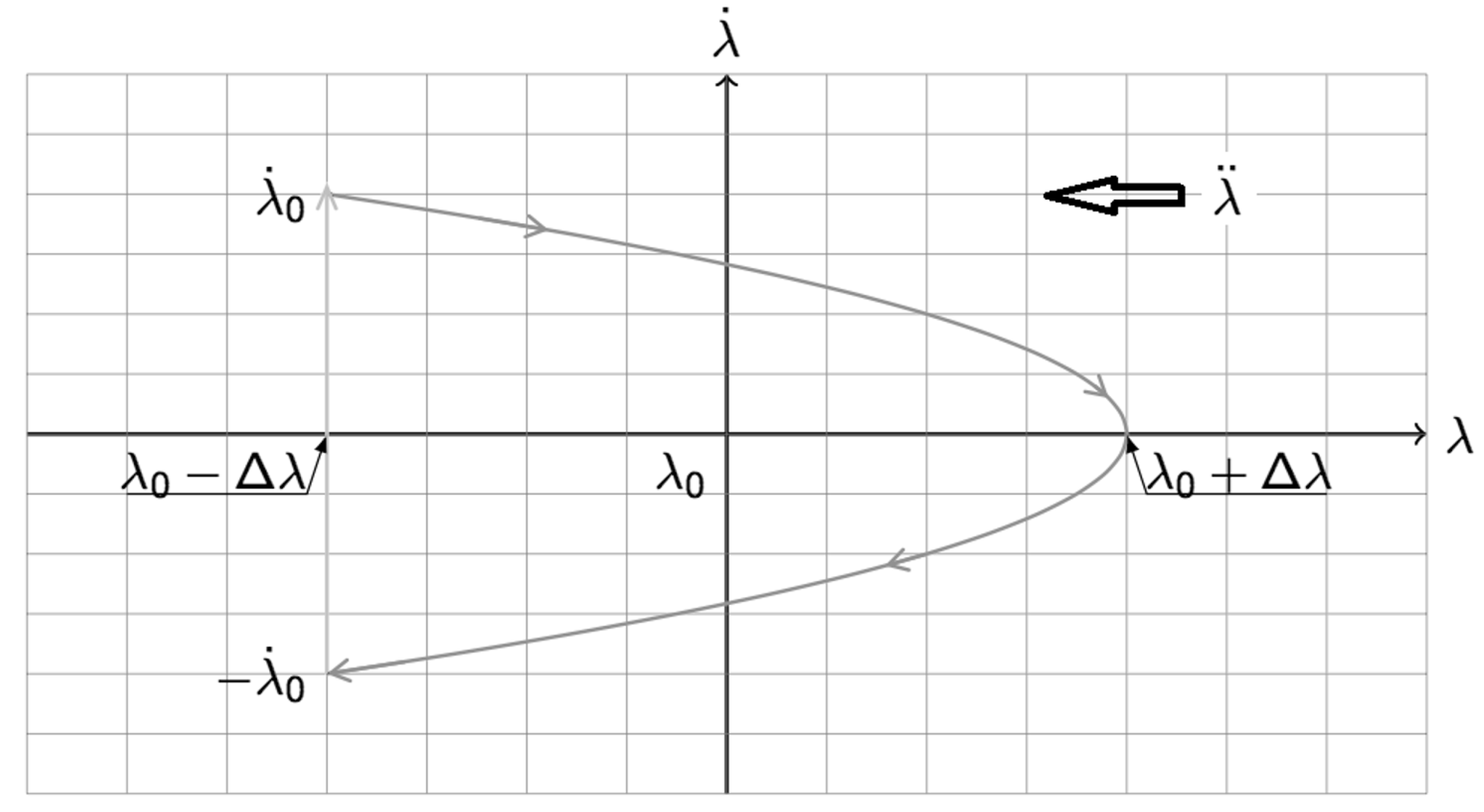
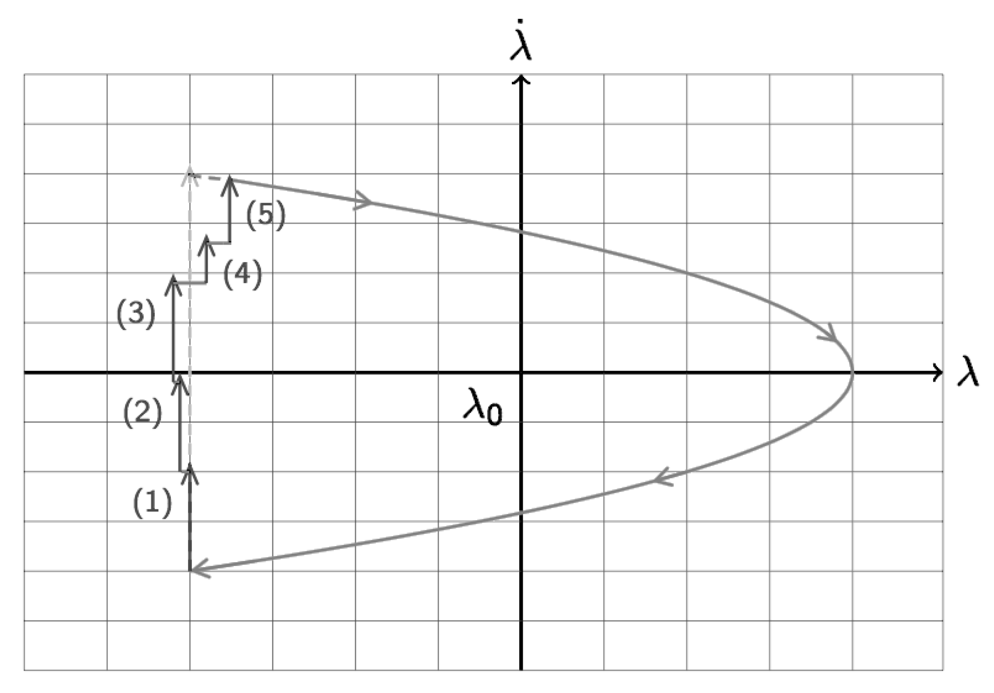
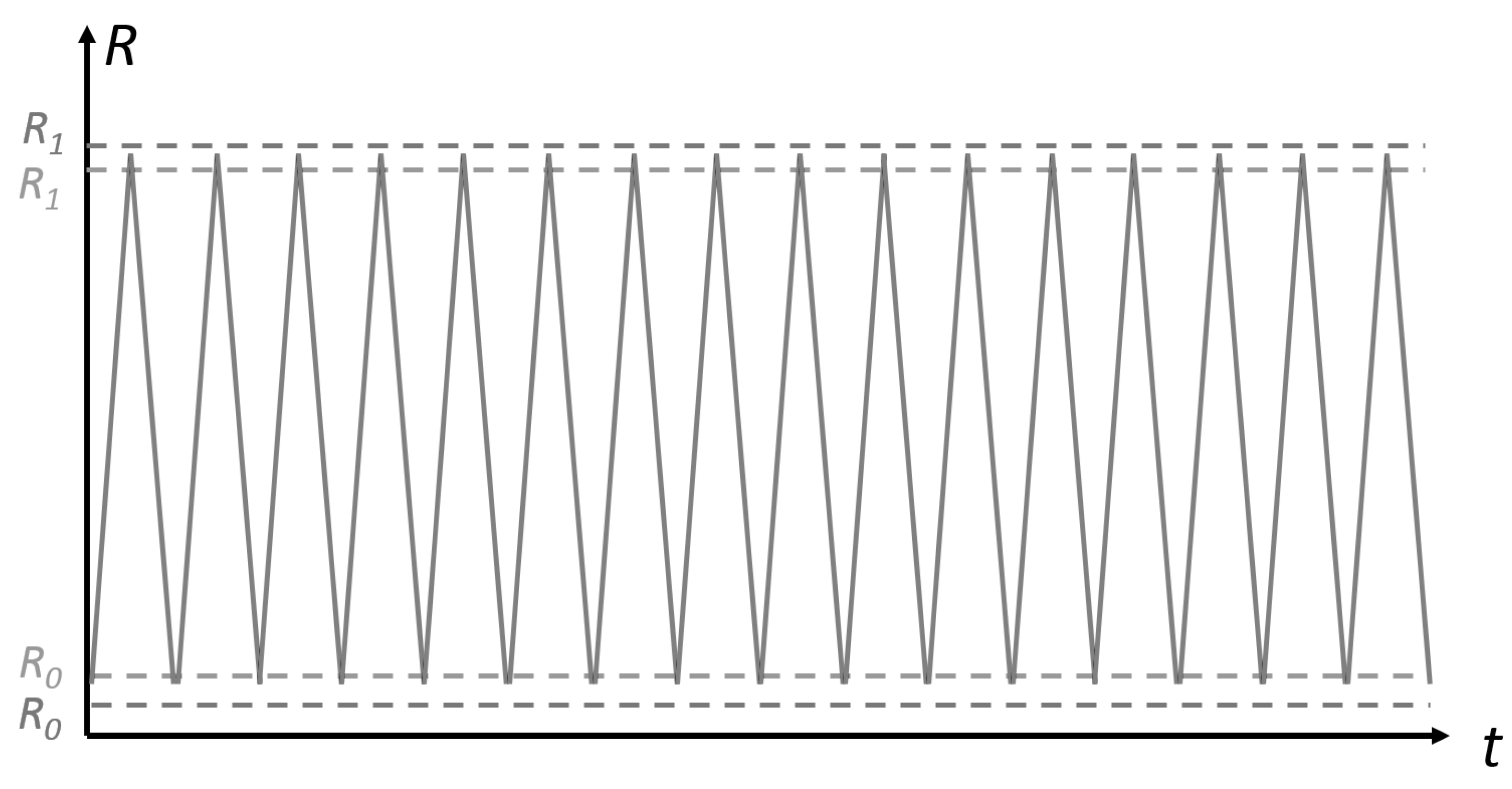
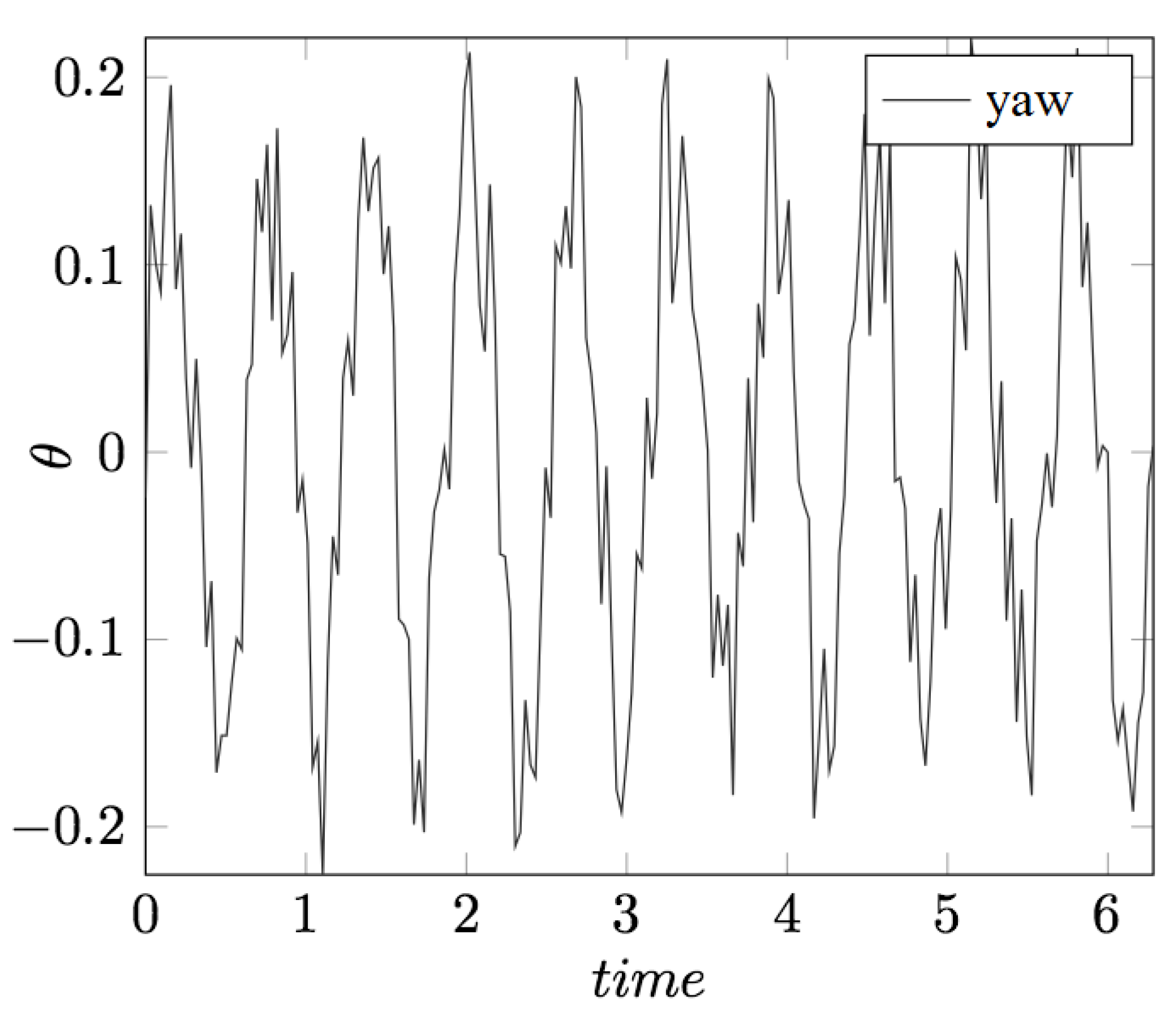
  • Thruster control: According to Euler’s moment equations, a thruster pulse in the correct direction from thruster T 1 or T 2 can increase the angular momentum of spacecraft about the + y ^ b or - y ^ b axis. With no active attitude control, the body accumulates angular velocity as the angular momentum of the spacecraft increases, changing the attitude of the spacecraft. However, if momentum wheels are used to stabilize the attitude, then the accumulated angular momentum will be transferred to the wheels. As shown in Figure 12, alternating the ignition of thruster T 1 or T 2 will produce cyclic variations in MW speed. In Figure 12, the lighter solid line indicates the increasing MW speed when T 1 fires, and the dark line is the decreasing MW speed when T 2 fires. R u and R l are the speed limits corresponding to the control overshoot limits R ^ u and R ^ l . Figure 13 demonstrates that the evolution of the yaw is bounded by the thrusting maneuvers. Therefore, it is possible to implement thruster attitude control while still keeping MW speed within acceptable bounds. The measured change in wheel speed induced by thruster firing can then be used to calculate the variation in the semi-major axis. Furthermore, this method works even under degraded thruster response.
    The whole process is shown in Table 1; a longitudinal or east–west thrust changes both the longitudinal drift rate and the eccentricity of the orbit. The net semi-major axis variation is 1 . 25 km, which produces a drift rate of D = - 0 . 016 deg/day. The maneuver provides good longitudinal correction while also ensuring that the attitude remains within bounds.
Figure 12. Momentum wheel (MW) rotation rate.
Aerospace 02 00581 g012
Figure 13. Yaw evolution.
Aerospace 02 00581 g013
Table 1. Simulation showing the correction of orbital elements using thruster firing.
FiringThruster Δ n w Δ a Δ λ ˙ | Δ e |
(rpm)(km)(deg/day)
1T21000 - 0.145 0.192 3.54 · 10 - 4
2T11000 - 0.149 0.186 3.44 · 10 - 4
3T21000 - 0.145 0.192 3.54 · 10 - 4
4T11000 - 0.149 0.186 3.44 · 10 - 4
5T21000 - 0.145 0.192 3.54 · 10 - 4
6T11000 - 0.149 0.186 3.44 · 10 - 4
7T21000 - 0.145 0.192 3.54 · 10 - 4
8T11000 - 0.149 0.186 3.44 · 10 - 4
9T2503 - 0.073 0.094 1.73 · 10 - 4

6. Workflow

In summary, the E–W station-keeping maneuver consists of the following four steps:
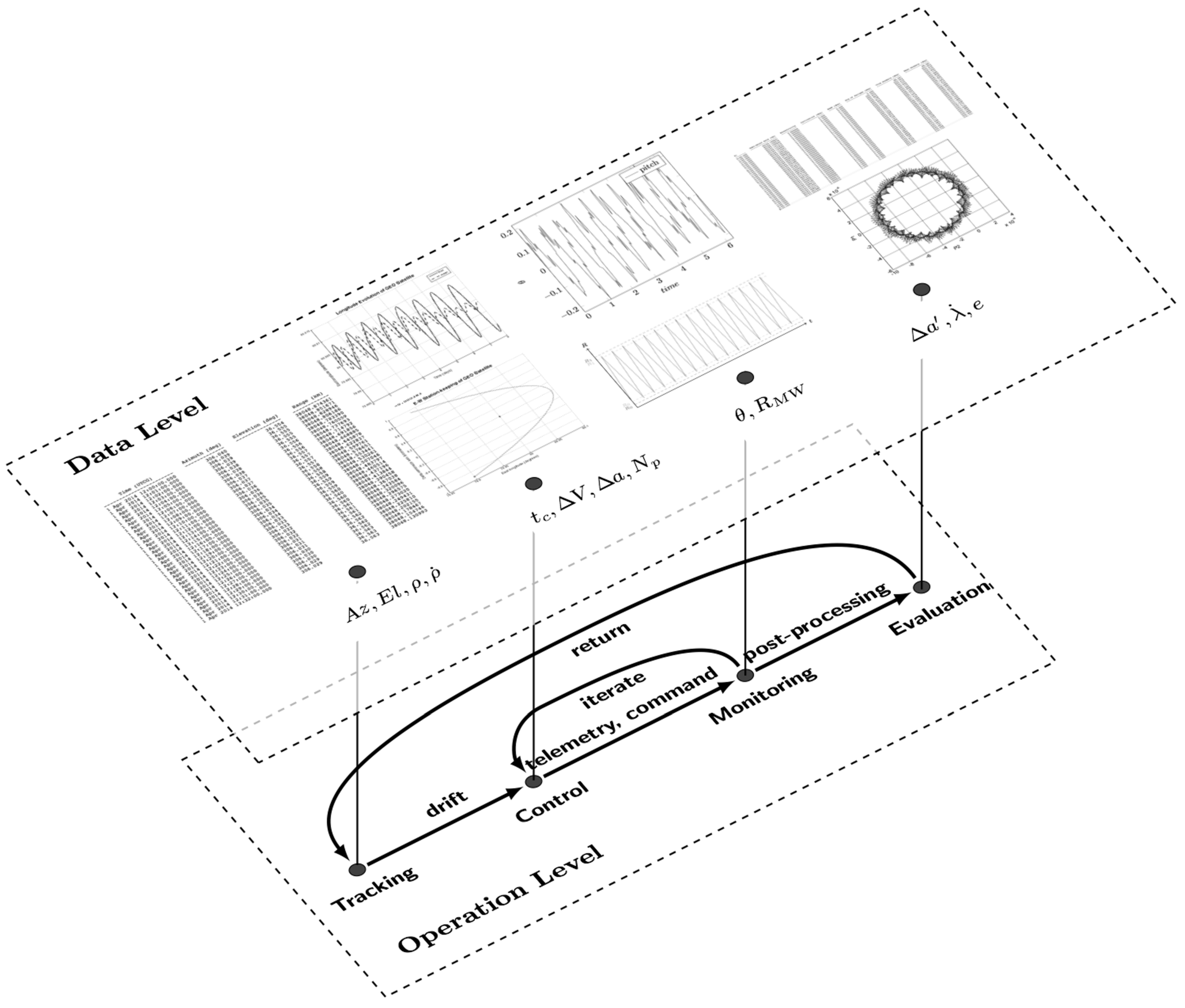
  • Step 1: Preliminary spacecraft tracking gives initial data consisting of range (ρ) and/or antenna angles azimuth ( A z ), elevation ( E l ) measured from one or more ground stations at discrete time points. The range rate ( ρ ˙ ) is of less interest for geostationary orbits. The precisely-determined and predicted orbit can be estimated using the most recent available tracking data.
  • Step 2: Subsequently, the prescribed longitude boundary must be used to design the E–W station-keeping maneuver. From the prescribed longitude boundary, the thruster ignition start time t c , the change of the semi-major axis Δ a , the executed velocity increment Δ V , the mean fuel consumption and other variables are calculated. Performing longitude maneuvers near apogee (or perigee), we can prevent eccentricity from becoming too great due to a single thrust. At the beginning, some short impulses (quarter or half width) are fired to evaluate the thrusters’ performance and to calibrate the system.
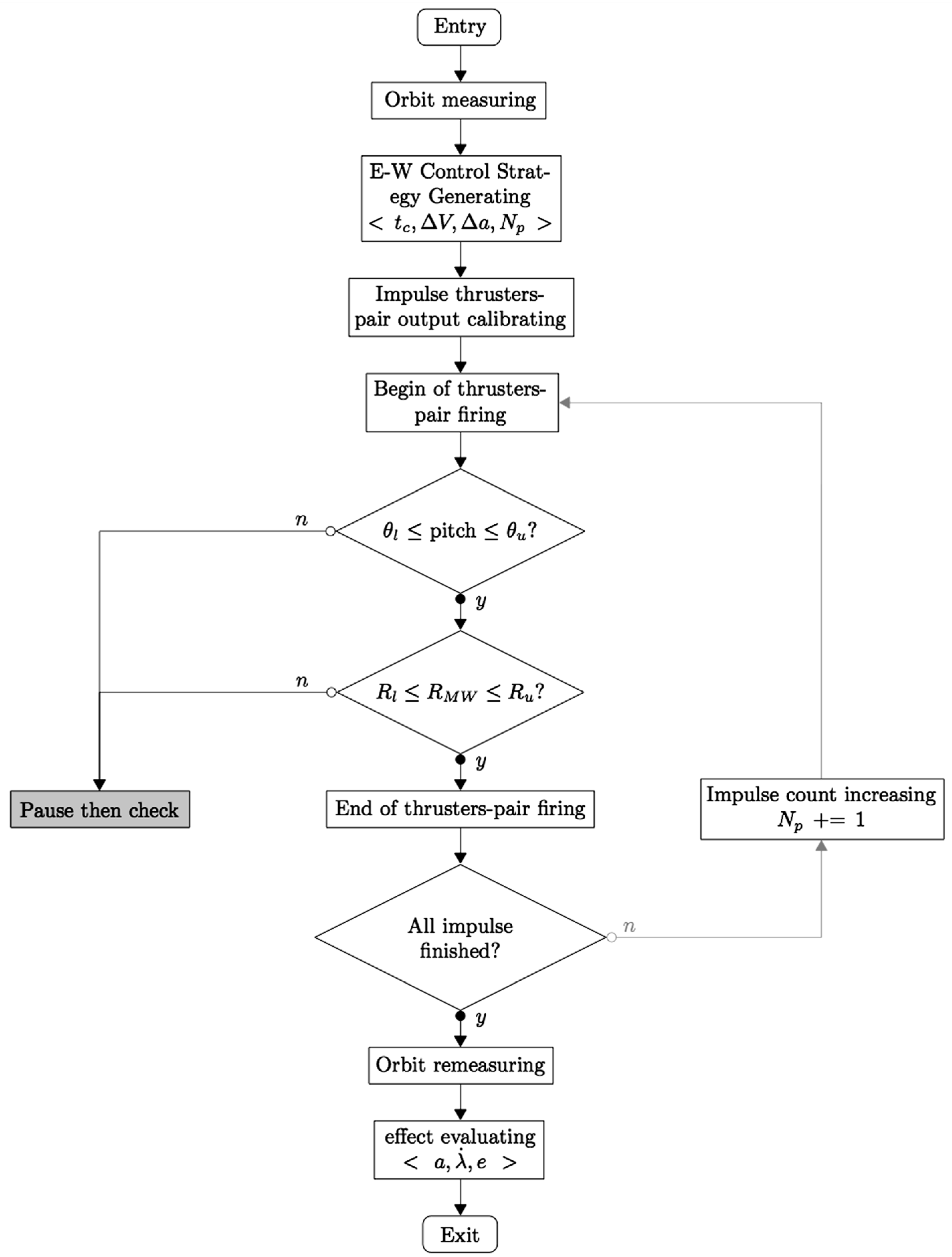
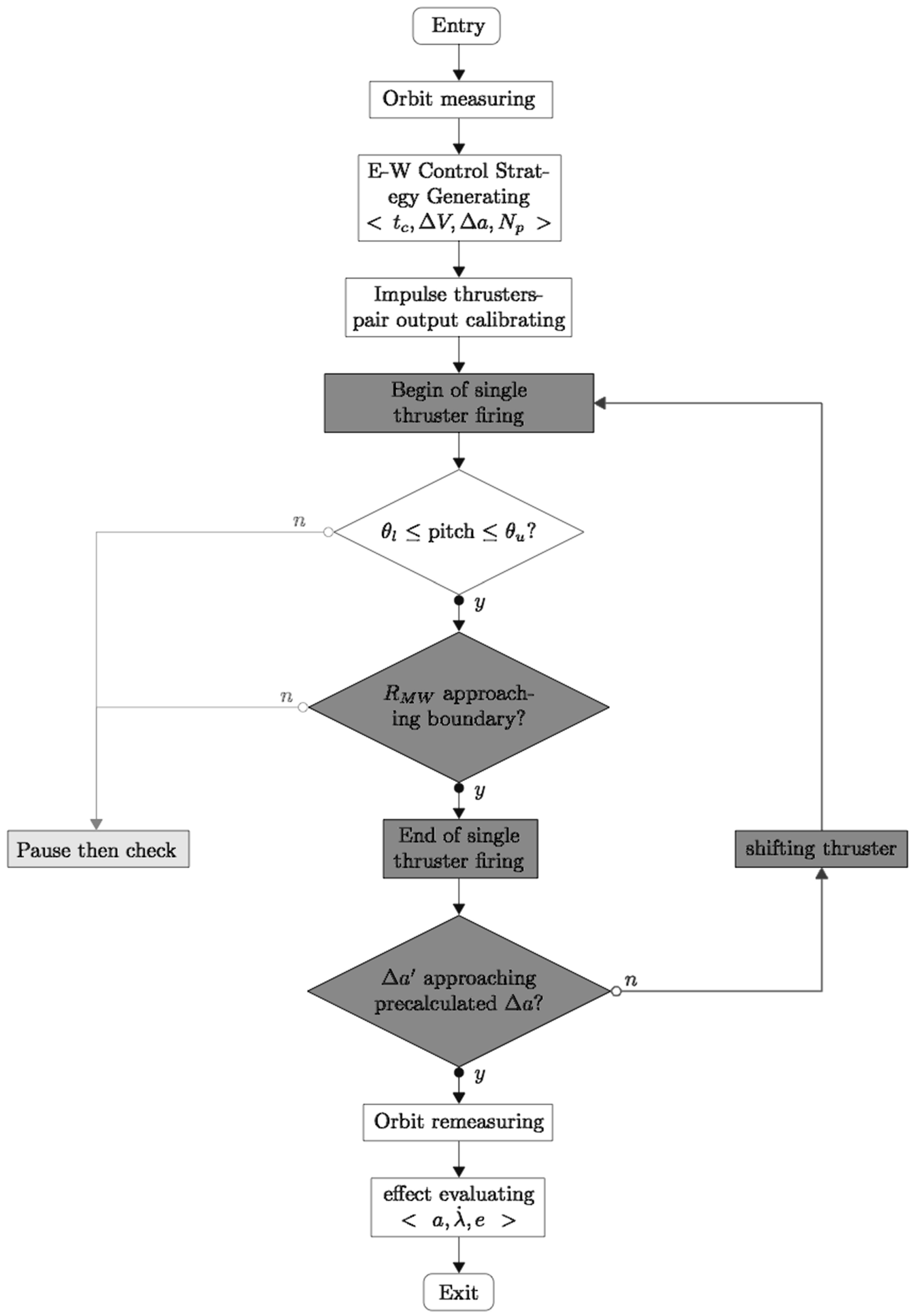
  • Step 3: Next, Figure 14 gives the workflow for performing station keeping assuming nominal thruster performance. At the start time t c , thruster pair T 1 , T 2 fires. In order to prevent large yaw attitude errors, the yaw θ must be monitored. Thruster firing must be modified when thruster performance is degraded. A modified workflow assuming degraded thruster performance is shown in Figure 15. The main difference between the nominal and modified workflow is marked with dark grey. Instead of simultaneous firing of thrusters T 1 and T 2 , firing is alternated, while keeping angular wheel velocity R M W between the lower and upper bounds. Furthermore, in order to prevent the wheel momentum from approaching the permitted limits, the length of single thruster firings must be confined. Moreover, the workflow loop termination condition is affected by how far Δ a is from its desired value.
  • Step 4: In the end, for orbit re-estimation, the new orbital elements can be determined from the latest tracking data. Through data post-processing, the updated orbital Δ a , D and e can be used to estimate the effect of the maneuver. Finally, the next station-keeping maneuver can be started with a new thruster firing scheme.
In reference to Figure 16, the modified workflow procedure can be conceptually divided into a “data level” and an “operation level”.
Figure 14. Nominal thruster workflow.
Aerospace 02 00581 g014
Figure 15. Modified workflow for degraded thruster performance.
Aerospace 02 00581 g015
Figure 16. Illustration of the workflow.
Aerospace 02 00581 g016

7. Conclusions

In this paper, we present an approach for longitudinal station keeping of a GEO satellite with degraded thrusters and with momentum wheels or gyros for attitude control. The approach introduces a procedure for station keeping that reduces the need for last minute contingency maneuvers being performed by satellite operators. A simulation implementing the proposed approach is presented with results summarized in Table 1. The results show that tight control of the orbital elements can be achieved with degraded thruster response when control moment gyros are used for correcting attitude dynamics and measuring deviations in the orbital elements. The proposed method requires more maneuvers to be performed in order to maintain correct station keeping. The extra maneuvers require more involvement from satellite operators on the ground with additional maneuver cost and risk increased. However, the need for last minute correction is reduced in the case of excessive longitudinal drift, especially for satellites near the unstable longitudinal nodes, which experience the most drift. Furthermore, tighter control minimizes excessive unwanted variation in orbital elements due to degraded thruster firing, thus providing higher quality communications. This increases mission robustness by ensuring that GEO satellites remain within the required operational deadband.

Author Contributions

Yunhe Wu has conceived of the problem and initially developed part of the derivations with the help of Daniele Mortari. Stoian Borissov has completed the theory and the derivations. Daniele Mortari has supervised in detail the theory and, along with Stoian Borissov, has improved the use of English in the manuscript.

Conflicts of Interest

The authors declare no conflict of interest.

References and Notes

  1. Circi, C. Simple Strategy For Geostationary Stationkeeping Maneuvers using Solar Sail. AIAA J. Guid. Control Dyn. 2005, 28, 249–253. [Google Scholar] [CrossRef]
  2. Shrivastava, S.K. Orbital Perturbations and Stationkeeping of Communication Satellites. J. Spacecr. Rockets 1978, 15, 67–78. [Google Scholar] [CrossRef]
  3. Lee, B.S.; Hwang, Y.; Kim, H.Y.; Park, S. East–West Station-Keeping Maneuver Strategy for COMS using Iterative Process. Adv. Space Res. 2011, 47, 149–159. [Google Scholar] [CrossRef]
  4. Romero, P.; Gambi, J.M. Optimal Control in the East–West Station-Keeping Manoeuvres for Geostationary Satellites. Aerosp. Sci. Technol. 2004, 8, 729–734. [Google Scholar] [CrossRef]
  5. This problem affects all satellites on compatible orbits (also called resonant orbits) and GEO satellites are in the 1-1 compatible orbit.
  6. Ostrander, N.C. Longitudinal Station Keeping of Nearly Geostationary Satellites; Rand Corporation: Santa Monica, CA, USA, 1969. [Google Scholar]
  7. Soop, E.M. Handbook of Geostationary Orbits; Springer: Dordrecht, The Netherlands, 1994; Volume 3. [Google Scholar]
  8. Crouch, P.E. Spacecraft Attitude Control and Stabilization: Applications of Geometric Control Theory to Rigid Body Models. Trans. IEEE Autom. Control 1984, 29, 321–331. [Google Scholar]
  9. Hardacre, S. Control of Colocated Geostationary Satellites; Cranfield University: Bedford, UK, 1996. [Google Scholar]
  10. Hughes, P. Spacecraft Attitude Dynamics; Courier Dover Publications: Mineola, NY, USA, 2012. [Google Scholar]
  11. Romero, P.; Gambi, J.M.; Patiño, E. Stationkeeping Manoeuvres for Geostationary Satellites using Feedback Control Techniques. Aerosp. Sci. Technol. 2007, 11, 229–237. [Google Scholar]
  12. Sidi, M.J. Spacecraft Dynamics and Control: A Practical Engineering Approach; Cambridge University Press: Cambridge, UK, 1997; Volume 7. [Google Scholar]

