Aerodynamic Effects of Measured Leading-Edge Geometric Deviations on Highly Loaded Low-Pressure Turbine Blades

Abstract

Geometric deviations can considerably degrade the aerodynamic performance of low-pressure turbine blades, especially as blade loading is increased for reduced blade count and weight. Stronger suction-side adverse pressure gradients then make the boundary layer more sensitive to leading-edge disturbances. In this work, 1781 measured leading-edge deviation samples are mapped onto the T106D-EIZ low-pressure turbine blade. The resulting profiles are compared with a Gaussian-process-based smooth deviation set. At the Zweifel coefficient Zw = 1.28, the measured deviations increase the mean loss by 5.1% relative to the nominal value, with a relative standard deviation of 14.2% and a 2.9% probability of a loss increase exceeding 30%. This impact is amplified at Zw = 1.30, where open suction-side separation occurs in 9.4% of the measured profiles. Leading-edge thickness variation is a major contributor to the loss variation. Leading-edge thinning strengthens the suction-side pressure spike, promotes local separation and transition, increases downstream friction loss, and weakens the boundary-layer momentum before the trailing edge. However, thickness reduction does not fully account for the high-loss risk observed in the measured profiles. For a pair with comparable leading-edge thickness, the loss coefficient is 0.1556 for the measured sample and 0.0469 for the corresponding smooth Gaussian process sample at Zw = 1.30. The additional risk is associated with measured local non-smoothness and irregular curvature variation, which disturb the leading-edge pressure-gradient development, increase suction-side cumulative loss and wake-mixing loss, and can trigger earlier large-scale separation. These results indicate that realistic leading-edge shape quality should be considered in tolerance assessment and robust aerodynamic design of highly loaded low-pressure turbine blades.

1. Introduction

Low-pressure turbines (LPTs) in civil high-bypass-ratio turbofan engines are continuously required to provide high aerodynamic efficiency with reduced blade count and module weight [1,2]. High-lift and ultra-high-lift blade designs offer an effective route to this objective by increasing the work output of each blade row. Practical aeroengine-related LPT developments have shown that increased blade loading can support compact turbine modules, with a 20% reduction in blade number reported for the BR715 high-lift LPT and an approximately 38% lift increase reported relative to Trent 700 blades [3,4,5,6]. However, the higher blade loading also produces a stronger suction-side acceleration and a more severe adverse pressure gradient. The suction-side boundary layer then becomes more sensitive to the leading-edge pressure spike and to the subsequent transition and separation processes. Under these conditions, small leading-edge geometric deviations may lead to a significant decline in aerodynamic performance [7,8]. Therefore, uncertainty quantification and risk assessment based on realistic leading-edge deviations are needed for highly loaded LPT blades [9].

Manufacturing geometric variations have been widely recognized as an important source of aerodynamic uncertainty in turbomachinery [7,10,11,12]. Previous studies on turbines and compressors have shown that geometric variability can cause overall performance deterioration, considerable performance scatter, and high-loss tail events [8]. Garzon and Darmofal delineated critical characteristics of the influence of machining deviations on compressor performance: overall performance decline, substantial scatter, and the risk of severe performance degradation [13]. Wang et al. further showed that for highly loaded low-pressure turbines, unfavourable geometric deviations, such as leading-edge thinning, can cause a pronounced deterioration in aerodynamic performance, whereas opposite deviations, such as leading-edge thickening, provide only limited aerodynamic benefit. As a result, the overall performance tends to degrade, and a clear high-loss risk appears, with nonlinear and non-Gaussian characteristics [14]. In addition, operational deterioration has been shown to increase the sensitivity of blade performance to random perturbations. For instance, Razaaly et al. [15], Wang et al. [16], and Guo et al. [17] showed that an increase in loading or incidence could considerably amplify this sensitivity to geometric variations. Bertini et al. also emphasized that as LPT aerodynamic loading increases in modern high-loading designs, blade performance becomes more sensitive to deviations from the design intent, including geometric variations, leading to reduced aerodynamic robustness [18]. Therefore, it is necessary to investigate the nonlinear uncertainty effects of geometric deviations on highly loaded LPTs and assess the consequent aerodynamic performance scatter and the risk of significant decline.

Previous studies have shown that geometric details and deviations in the leading-edge region have a significant aerodynamic impact [19,20]. For example, Davis pointed out that the curvature continuity between the leading edge and the main body directly affects the pressure spike and significantly changes the local boundary-layer flow [21]. Hodson et al. [22] emphasized the importance of transition and separation near the leading edge in determining the subsequent development of the suction-side boundary layer over turbine blades. Benner [23] also reported that the leading-edge geometry of turbine blades, especially the curvature continuity between the leading edge and the blade surface, has a strong nonlinear influence on the leading-edge flow. Zhang et al. [24] weakened the pressure spike and suppressed the leading-edge separation bubble on the suction side by optimizing the leading-edge profile of a turbine blade, leading to an efficiency improvement of approximately 0.6% in a five-stage low-pressure turbine. Leading-edge geometric deviations can also have a pronounced effect [25]. Ma et al. investigated the influence of real leading-edge manufacturing errors on the aerodynamic performance of a high-subsonic compressor cascade and showed that the total-pressure loss is highly sensitive to leading-edge errors, especially at high incidence [26]. Wang et al. similarly indicated that local geometric deviations, such as leading-edge thickness variations, strongly affect the suction-side boundary-layer flow and loss of turbine blades and that this effect is significantly amplified as the aerodynamic loading increases [14]. These studies indicate that the leading-edge region should be treated as a key source of aerodynamic sensitivity when realistic manufacturing deviations are assessed for highly loaded LPT blades.

Regarding research on the aerodynamic impact of geometric deviations, uncertainty modelling of geometric deviations is essential for generating sufficient profile samples for subsequent quantitative analysis. The key requirement is to represent the real-world characteristics of manufacturing deviations, and a sufficient number of measured blade geometries provides an important basis for this modelling [27,28]. Garzon and Darmofal introduced a principal component analysis (PCA) model for the decomposition, analysis, and reconstruction of measured geometric variations, representing a pioneering study on the systematic quantitative assessment of the effects of overall profile variations on turbomachinery performance [13]. Owing to the limited availability of measured blade geometries, several studies have focused on prescribed probability distributions of geometric variations [7]. For example, a Gaussian-process-based random field can represent smooth spatially correlated perturbations with a prescribed standard-deviation distribution. This model can produce numerous smooth and continuous profile samples and is also compatible with PCA-based deviation modelling, which is commonly used in geometric deviation modelling [29]. However, measured geometric deviations may contain non-ideal local features that are difficult to represent using smooth stochastic processes, and deviation models based on selected parameter distributions may underestimate the risk associated with actual deviations outside the prescribed parameter space. For example, Wang et al. indicated that manufacturing deviations can introduce pronounced non-smooth geometric errors near the leading and trailing edges, which can directly increase aerodynamic loss, but are difficult to represent using a Gaussian process model [30]. Similarly, Li et al. showed that PCA-type low-order deviation models may omit aerodynamically sensitive but low-variance geometric modes and therefore underestimate the scatter of aerodynamic performance, emphasizing the importance of using measured deviations directly for reliable robustness assessment [31,32]. As a result, considering the LPT design trend with increasingly high loading, it is necessary to assess the high-loss risk induced by measured manufacturing deviations in order to effectively evaluate aerodynamic robustness in real operating conditions.

Previous studies have shown that leading-edge geometry can strongly affect turbine boundary-layer development. However, the aerodynamic response to measured leading-edge deviations under high loading has not been fully quantified. In measured profiles, leading-edge deviations may include both thickness changes and local shape irregularities in the leading-edge region, and their respective aerodynamic roles remain unclear. Accordingly, this work aims to quantify the loss and separation response of a highly loaded LPT blade to measured leading-edge deviations and to clarify how thickness variation and local shape irregularity contribute to this response. The measured deviations are mapped onto a common T106D-EIZ profile, and a Gaussian-process-based smooth deviation set is constructed as a reference. The analysis is arranged from statistical response to flow mechanism. First, the load-dependent aerodynamic response of the measured leading-edge deviations is quantified. Second, the role of leading-edge thickness is examined by comparing the measured profiles with the smooth reference set. Finally, representative measured and smooth profiles with comparable leading-edge thickness are compared. This final comparison is used to clarify the effects of local non-smoothness and irregular curvature variation on suction-side boundary-layer development and loss generation. Through this progression, the role of realistic leading-edge shape quality is assessed for tolerance evaluation and robust aerodynamic design of highly loaded LPT blades.

2. Methods

A comparative computational framework is used to isolate the aerodynamic effects of measured leading-edge deviations. The T106D-EIZ blade profile is first used as a common reference geometry, and measured wall-normal deviations are mapped to its leading-edge region. A smooth Gaussian-process-based deviation set with comparable pointwise magnitude is then generated as a reference. The measured and smooth deviation sets are evaluated under identical CFD settings and loading levels so that the load-dependent response, the thickness-related trend, and the additional effect of measured local shape irregularity can be compared consistently.

2.1. Research Object and CFD Method

The T106D-EIZ profile [33] is adopted as the reference highly loaded LPT blade. The profile and curvature distribution are shown in Figure 1, where a regular and continuous curvature distribution can be observed. This profile is selected because it has publicly available experimental data for numerical validation and has been widely used in studies of LPT transition and separation. In the T106D-EIZ test case, the pitch-to-chord ratio was increased to 1.05, which increased the lift coefficient by approximately 30% and produced a large suction-side separation bubble [33]. Therefore, this profile is a suitable benchmark for studying the aerodynamic sensitivity of highly loaded LPT blades. In the present study, the chord length is set to b = 30 mm. Three pitch settings are applied while the blade profile is kept unchanged, corresponding to Zweifel coefficients Zw = 1.25, 1.28, and 1.30. This range is selected to represent a high-loading regime relevant to high-lift LPT design studies [5,6].

The basic operating condition follows the Point 2 condition of the T106D-EIZ test case reported in ref. [33]. The inlet total temperature, inlet total pressure, outlet static pressure, inlet flow angle, and inlet turbulence intensity are listed in

Table 1. Main operating parameters for the basic condition.

Parameter	Value
Inlet total temperature	287 K
Inlet total pressure	5.7 × 104 Pa
Outlet static pressure	4.5 × 104 Pa
Inlet flow angle	37.7°
Inlet turbulence intensity	2.5%

. Based on the chord length and the exit velocity under isentropic expansion, the outlet Reynolds number is approximately 2.0 × 10⁵ and the outlet Mach number is approximately 0.59. The total-pressure loss coefficient, denoted by ζ, is used as the main aerodynamic performance parameter and is defined by Equation (1), where P_ti is the inlet total pressure and P_to and P_so are the outlet total pressure and outlet static pressure, respectively.

$$\zeta ={\displaystyle \frac{P_{\mathrm{ti}}-P_{\mathrm{to}}}{P_{\mathrm{to}}-P_{\mathrm{so}}}}$$

(1)

The aerodynamic performance is simulated using the 2D steady Reynolds-averaged Navier–Stokes solver MAP [34]. This solver supports automated case setup, mesh generation, and flow-field solution, making it suitable for the large-scale numerical simulations of the impact of geometric deviations on LPT aerodynamic performance in this work. The shear stress transport (SST) turbulence model is coupled with the γ-Re_θt transition model to predict the transition and separation behaviour of the LPT boundary layer. As shown in Figure 2, the computational domain consists of one 2D blade passage, with the inlet and outlet boundaries located one axial chord upstream of the leading edge and two axial chords downstream of the trailing edge, respectively. A static, body-fitted structured mesh is generated independently for each blade geometry. Six meshes with the same topology and grid-point numbers ranging from 1.74 × 10⁴ to 4.34 × 10⁴ are used for the grid-independence assessment. All wall-adjacent grid points are arranged with y⁺ below 1. The assessment included the nominal profile at Zw = 1.28, a representative thin-leading-edge profile at Zw = 1.28, and the same thin-leading-edge profile at Zw = 1.30. The last case exhibits a large-scale open separation and provides a more demanding test of grid sensitivity. As shown in Figure 3, ζ decreases monotonically with increasing grid density. Beyond Grid 4, the differences in ζ are approximately 0.0005–0.0010 for the first two cases and approximately 0.002 for the open-separation case. These differences remain substantially smaller than the loss variations among the representative geometries. The distributions of the surface isentropic Mach number Ma_is derived from Grid 4, Grid 5, and Grid 6 are also closely matched. Therefore, Grid 4 is adopted for the large-sample calculations in this work, and the total grid number is 3.17 × 10⁴.

The CFD method is further assessed against published T106D-EIZ experimental data under the Point 2 and Point 3 conditions [33]. The comparison of the surface isentropic Mach number Ma_is in Figure 4 indicates that the main surface-loading characteristics, including the pressure spike, the suction-side pressure distribution, and the pressure plateau and recovery associated with boundary-layer separation, can be predicted with sufficient accuracy. The comparison supports the capability of the numerical method to reproduce the principal loading and separation characteristics over the investigated operating range.

Additional 3D calculations are conducted to assess the applicability of the 2D simplification. A straight linear cascade with an aspect ratio of 3 is constructed using the same blade section. The nominal and thin-leading-edge profiles are examined at selected Zw values covering both a small closed separation bubble and large-scale open separation. The operating conditions, turbulence and transition models, and numerical settings are kept consistent with those used in the 2D calculations. The hub and shroud are treated as no-slip walls, and the 3D mesh contains approximately 2.1 × 10⁵ grid points with 81 layers in the spanwise direction. For all examined cases, the midspan total-pressure loss coefficients predicted by the 2D and 3D simulations differ by less than 3%. The distribution of surface Ma_is is compared in Figure 5. It can be seen that the main loading characteristics are closely reproduced, and the change from limited separation to large-scale open separation as the loading is increased is identified in both simulations. These comparisons support the use of the 2D framework for assessing the effect of geometric deviations on the relative trend of profile loss and high-risk geometry identification.

The present work focuses on the effect of leading-edge geometric deviations on profile loss. Based on the above experimental comparison, grid-independence assessment, and 2D–3D comparison, the 2D steady framework retains the principal loading differences and separation regimes among the representative geometries. It is therefore adopted for the large-sample aerodynamic evaluation. The conclusions are restricted to profile-loss trends and do not include endwall and secondary-flow losses. The additional 3D calculations are limited to selected representative cases because of the high computational cost. The off-design incidence analysis in Section 3.1 is performed for all 1781 measured-deviation samples at Zw = 1.28, with two representative incidence angles, −3° and +3°, selected to examine the response under negative and positive-incidence conditions. Broader 3D verification and off-design assessments over more cases and operating conditions are left for future work.

2.2. Mapping of Measured Leading-Edge Deviations

The measured leading-edge deviation database is obtained from the turbine blade measurement data reported in the previous research work [30]. The measured object is a low-pressure turbine rotor blade from a small gas turbine engine, and the chord length of the measured blade section is approximately 20 mm. The surface profiles of 1781 manufactured blades are measured using a coordinate measuring machine, with a measurement error of approximately 0.01 mm. In this study, the leading-edge deviation patterns of these measured profiles are mapped onto the T106D-EIZ reference profile so as to evaluate the aerodynamic effects of realistic measured deviations under a common highly loaded LPT configuration.

Because the source profile is different from the T106D-EIZ reference profile in global shape and scale, the measured deviation is first expressed as a scalar wall-normal displacement relative to its own nominal profile. This representation separates the local manufacturing deviation from the absolute coordinate system of the source blade and allows the deviation to be transferred to another blade profile.

The deviations are mapped according to the relative surface circumferential position along the blade contour. The surface circumferential coordinate s is defined as a signed surface arc-length coordinate on the 2D blade profile. The leading-edge point is taken as s = 0. The positive and negative directions are taken along the pressure side and suction side, respectively, and |s| represents the arc length from the leading-edge point to the local surface point along the corresponding blade surface. For plotting, a relative circumferential position S is used and defined as S = (1 + s/L) × 100%, where L is the profile perimeter, as shown on the horizontal axis in Figure 6a. The leading-edge region is determined based on the signed surface arc-length coordinate of the nominal T106D-EIZ profile. Starting from the leading-edge point, the region extends to S = 109.7% on the pressure side and to S = 90.0% on the suction side. This region covers the curvature-dominated leading-edge portion and excludes the main blade-body region. The leading-edge thickness t is defined as the Euclidean distance between the pressure-side and suction-side boundary points of the leading-edge region. The normalized leading-edge thickness t/b is used in the following analysis.

For each measured sample, the wall-normal deviation distribution is resampled to the discrete surface points of the T106D-EIZ profile. The mean deviation is removed so that the mapped samples mainly reflect random manufacturing variation rather than a systematic offset. A scale factor of 2.0 is then applied to match the representative tolerance level of the reference blade size. The measured source blade has a chord length of approximately 20 mm, and the characteristic leading-edge wall-normal deviation level is approximately 0.1 mm. For the present T106D-EIZ reference profile with b = 30 mm, a representative profile tolerance of 0.2 mm is adopted according to the machining handbook [35,36]. Therefore, the measured deviations are scaled by 2.0 before being imposed on the reference profile. In this way, the mapped deviations preserve the measured local shape characteristics while remaining consistent with a realistic tolerance level for the target LPT leading edge.

Only the leading-edge region is perturbed in the present study because the objective is to isolate the aerodynamic influence of measured leading-edge geometry. In the marginal area of the leading edge, the imposed deviation is smoothly reduced to zero through a finite transition zone. This treatment avoids an artificial discontinuity between the perturbed leading edge and the unperturbed blade body. The final surface coordinates of the i-th perturbed profile are obtained by imposing the mapped normal displacement on the nominal profile as Equation (2), where x₀(s) is the nominal surface coordinate vector, n₀(s) is the outward unit normal vector vector, δ_i(s) is the scaled signed wall-normal deviation of the i-th measured sample, and w(s) is a dimensionless window function used to retain the leading-edge deviation and gradually suppress it to zero outside the leading-edge region. Therefore, the mapped profiles are used to evaluate the aerodynamic sensitivity to measured leading-edge deviation patterns on a common LPT reference profile. The circumferential distributions of the mapped measured deviations are shown in Figure 6a, and the resulting profile samples with applied leading-edge deviations are shown in Figure 6b. The pointwise standard deviation used for the Gaussian process model is compared in Figure 7a.

$${\mathit{x}}_i\left(s\right)={\mathit{x}}_0\left(s\right)+w\left(s\right){\delta }_i\left(s\right){\mathit{n}}_0\left(s\right),i=1,2,\dots ,1781$$

(2)

2.3. Gaussian-Process-Based Smooth Leading-Edge Deviation Model

A Gaussian-process (GP)-based smooth deviation model is constructed as a reference set with a pointwise deviation level comparable to that of the mapped measured deviations. This reference set is used to examine how much of the aerodynamic response can be represented by spatially smooth leading-edge perturbations. It is not intended to reproduce the local non-smoothness and irregular curvature variation observed in the measured profiles. Therefore, comparison between the measured-deviation set and the smooth GP reference set helps identify the additional aerodynamic effects associated with realistic local leading-edge shape irregularity.

The wall-normal deviation in the leading-edge region is modelled as a zero-mean GP along the signed surface circumferential coordinate s. The pointwise standard deviation σ(s) is specified according to the measured-deviation statistics after mapping. Since the objective of the GP model is to provide a spatially smooth reference set, a local smoothing treatment is applied to the narrow standard-deviation spike near the leading-edge point. The standard-deviation distribution away from this local spike is kept unchanged. The resulting smoothed distribution preserves the overall magnitude level of the measured deviations while avoiding the direct introduction of highly localized measured irregularities into the smooth reference model. The original and smoothed standard-deviation distributions are compared in Figure 7a. This smoothing treatment is applied only to construct the Gaussian process reference set, while the measured-deviation samples used in the aerodynamic simulations are not smoothed.

A squared-exponential covariance kernel cov is used to impose spatial smoothness between point s and point s’ along the leading-edge arc, as given in Equation (3). The distance between the two points is normalized by the chord length b, and the coefficient in the exponential term, −5, is selected following the smooth deviation model used in ref. [8]. The same leading-edge window function w(s) and the same transition treatment used for the measured deviations are applied to the GP samples. Further, the covariance matrix of the wall-normal deviations is constructed at the discrete leading-edge surface points. The covariance matrix is then decomposed using a PCA representation [13], and the random coefficients of the retained modes are sampled by Latin hypercube sampling to generate 400 smooth GP-based leading-edge profiles. The resulting profile samples with applied leading-edge deviations are shown in Figure 7b. Compared with the measured-deviation samples in Figure 6b, the GP-based profiles have a similar pointwise deviation level but are smoother and contain less local waviness. Therefore, under the present settings, the response difference is mainly related to the difference between measured local irregularity and smooth stochastic deviation.

$$\mathrm{cov}\left(s,s^{\prime }\right)=\sigma \left(s\right)\sigma \left(s^{\prime }\right)\exp \left[-5{\left({\displaystyle \frac{s-s^{\prime }}{b}}\right)}^2\right]$$

(3)

3. Results and Discussion

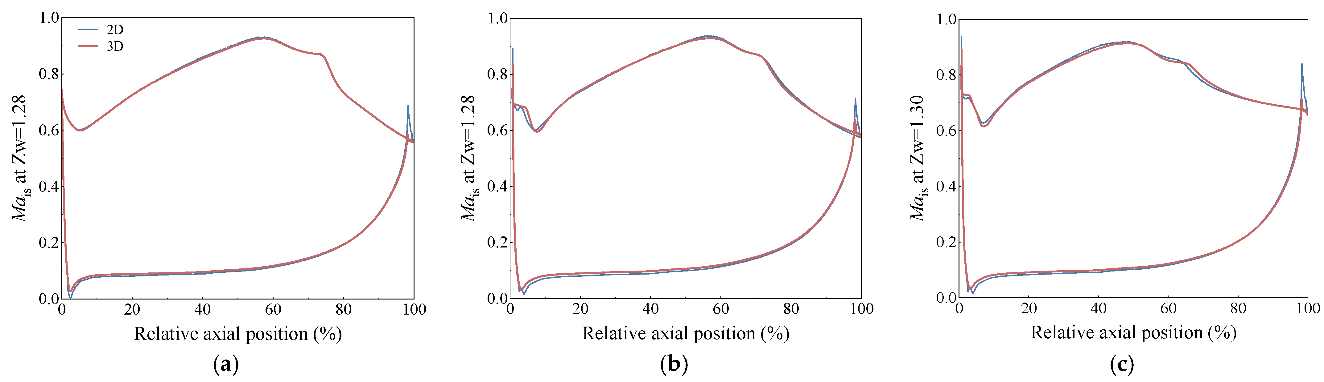
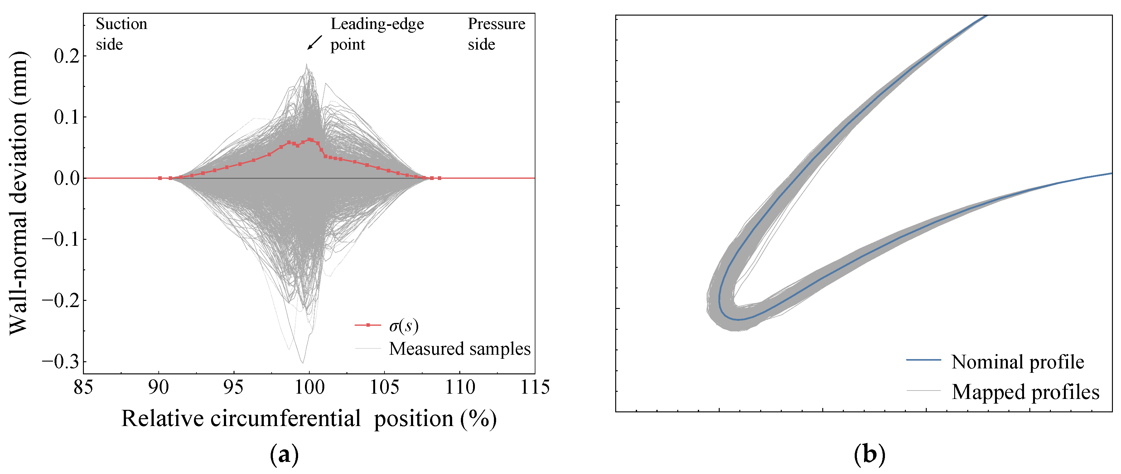
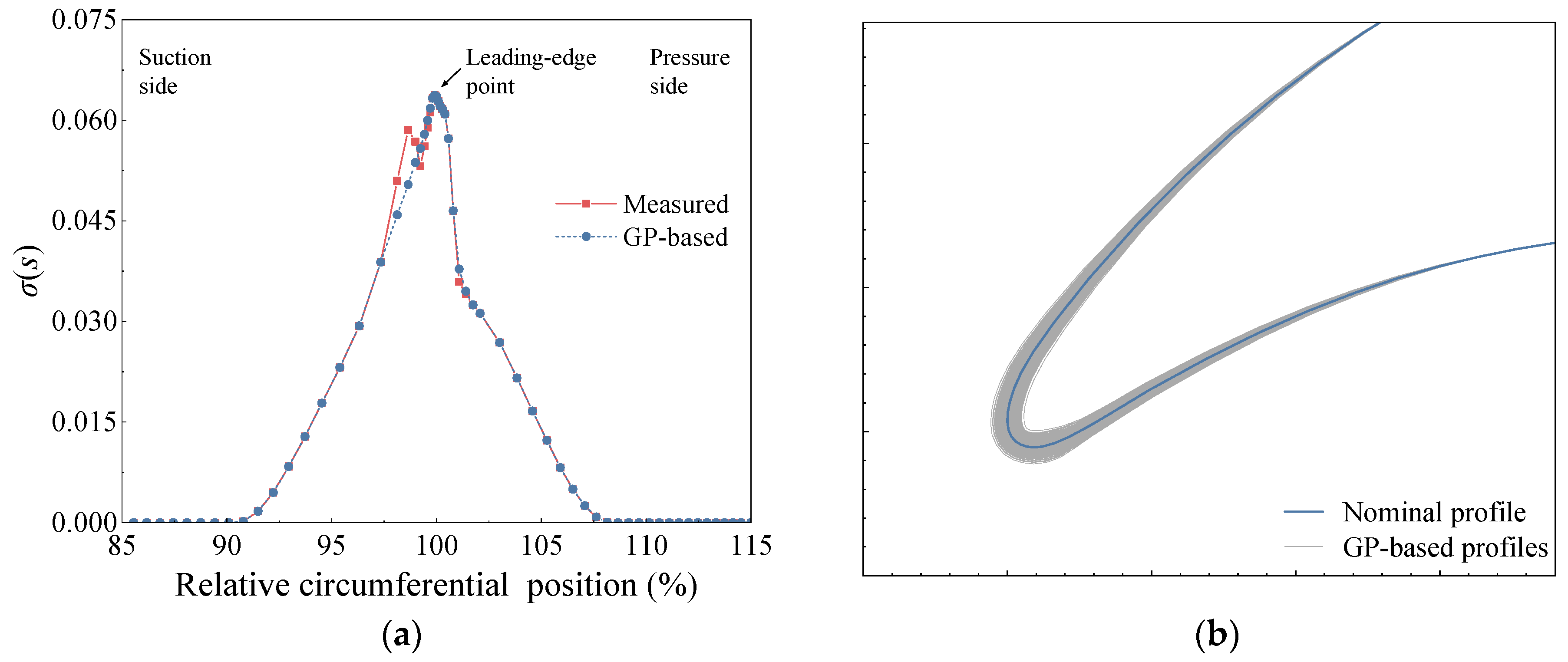
The aerodynamic influence of leading-edge deviations is discussed through a progressive analysis from overall loss statistics to local flow mechanism. The measured-deviation samples are first used to quantify the load-dependent changes in mean loss, loss scatter, high-loss tail risk, and open-separation occurrence. The results are then compared with those of the smooth GP-based deviations so that the response caused by smooth thickness-related perturbations can be distinguished from that caused by measured local shape irregularity. After this overall comparison, the relationship between leading-edge thickness and loss is examined to identify the first-order geometric trend. The remaining loss under comparable thickness is then analysed using representative measured and GP-based samples. This sequence is used to connect measured leading-edge geometry, local loading and pressure-gradient variation, suction-side boundary-layer development, and final loss formation.

3.1. Aerodynamic Impact of Measured Leading-Edge Deviations

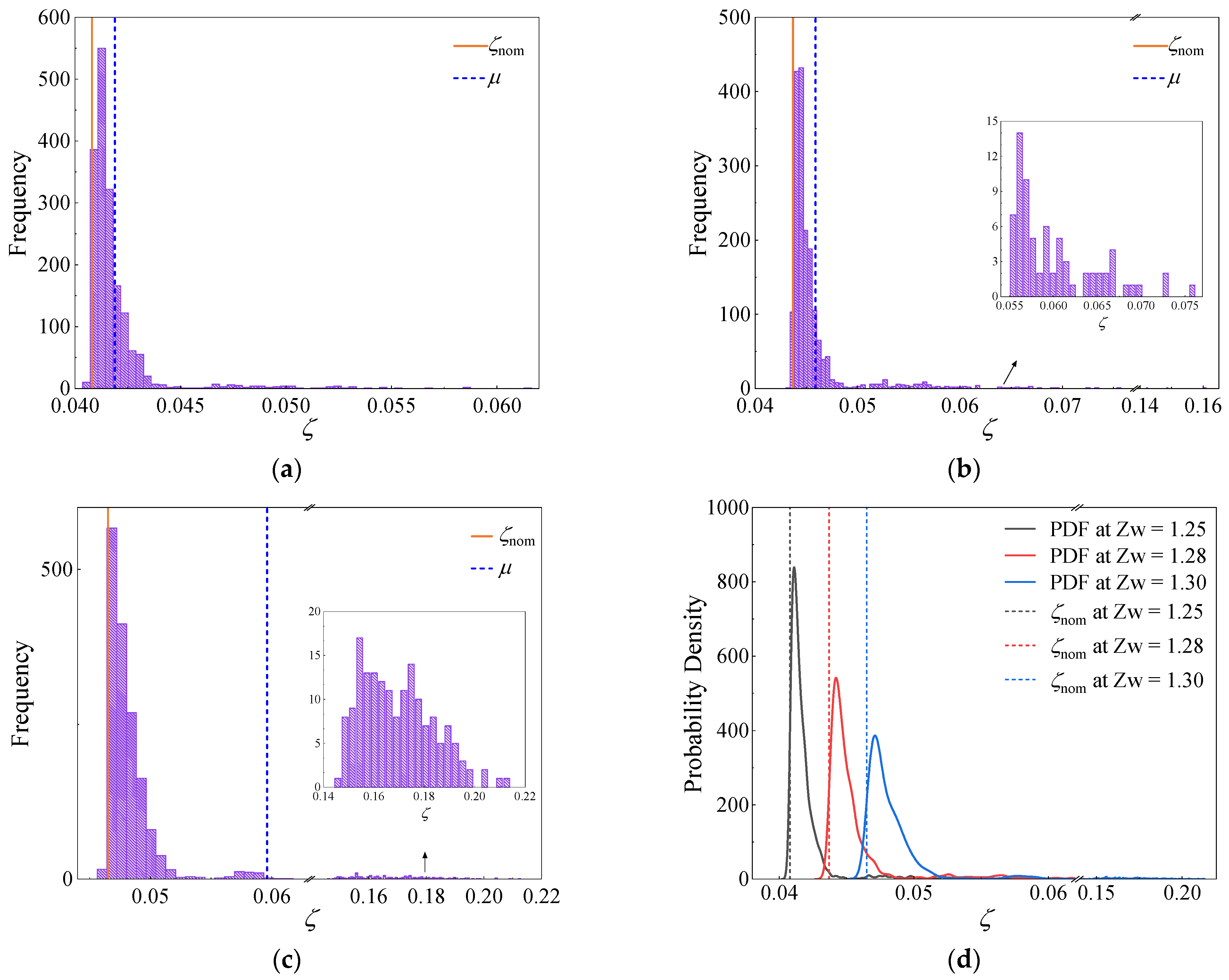
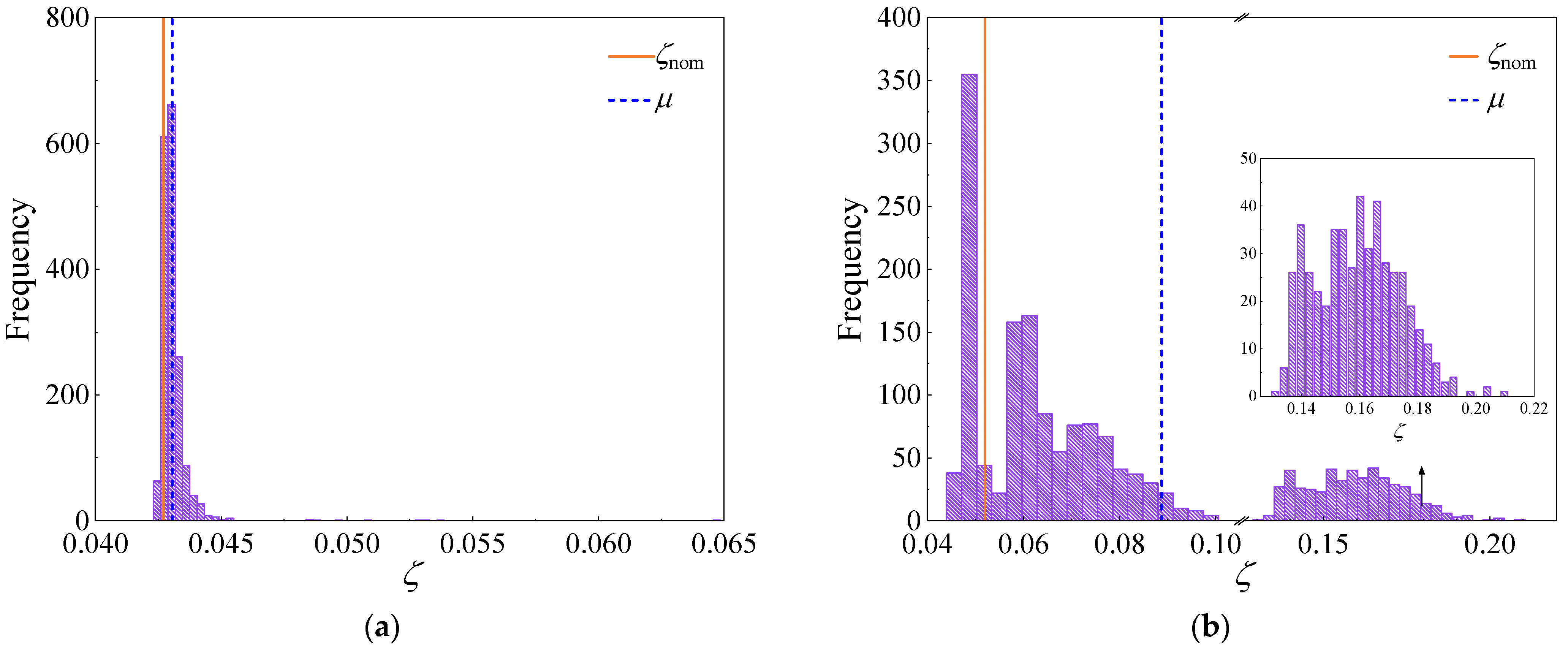
The computed loss ζ for the nominal T106D-EIZ geometry (ζ_nom) and the 1781 cases with measured leading-edge geometric deviations at the three loading levels are shown in Figure 8. The corresponding statistics are summarized in

Table 2. Aerodynamic statistics of measured leading-edge deviation samples under different loading levels.

Zw	ζnom	μ	σ/ζnom	Skewness	Kurtosis	P(Δζ/ζnom > 20%)	P(Δζ/ζnom > 30%)	Open-Separation Samples
1.25	0.0408	0.0419	4.6%	5.0	33.3	2.0%	0.6%	0
1.28	0.0437	0.0459	14.2%	12.5	208.8	6.1%	2.9%	4 (0.2%)
1.30	0.0465	0.0596	77.0%	2.8	9.3	11.7%	9.5%	168 (9.4%)

. The mean, standard deviation, and probability density curve of ζ are abbreviated as μ, σ, and PDF, respectively. The histograms indicate that ζ is strongly affected by the leading-edge geometric deviations. This effect is reflected by an overall increase in loss, a broader sample-to-sample scatter, and a pronounced upper-tail risk. A clear loading dependence is observed, and the deviation-induced loss penalty becomes more severe as the loading increases.

At Zw = 1.25, the mean value of loss, μ, increases by 2.7%, and the relative standard deviation, σ/ζ_nom, is 4.6%. Most samples remain close to ζ_nom. However, a distinct right-skewed tail is observed in the histogram. The skewness and kurtosis are much higher than the values of 0 and 3 associated with a Gaussian distribution, respectively, indicating a right-skewed distribution with a non-negligible upper tail. This shows that the response to measured leading-edge deviations is already nonlinear at Zw = 1.25, although most samples still remain close to the nominal loss level. These results suggest that the effect of measured leading-edge deviations is nonlinear. Deviations that are detrimental to aerodynamic performance can cause a strong increase in ζ, and their effects cannot be offset by deviations in the opposite direction. Consequently, a non-Gaussian distribution is obtained, with a mean value higher than the nominal loss and a noticeable risk of performance deterioration. This nonlinear response becomes more evident at higher loading. At Zw = 1.28, the mean profile loss increases by approximately 5.1% relative to the nominal value, and the standard deviation reaches 14.2% of the nominal value. The probabilities of a loss increase larger than 20%, 30%, and 40% are approximately 6.1%, 2.9%, and 1.3%, respectively. It is also noted that open separation appears in the adverse-pressure-gradient region on the suction side for four samples, and the loss rises abruptly to approximately 0.15. When the loading is further increased to Zw = 1.30, the distribution becomes much broader, and a distinct high-loss group appears. The mean value of ζ increases by 28.2%, and the relative standard deviation reaches 77.0%. The large increases in the mean loss and standard deviation are mainly caused by the enhanced nonlinear effect of the deviations, since many deviation cases lead to severe loss growth. In total, 168 samples, corresponding to approximately 9.4% of the measured-deviation set, exhibit open separation on the suction side. As a result, a bimodal loss distribution is formed, depending on whether open separation occurs. The aerodynamic performance is therefore severely degraded for this subset of manufactured geometries.

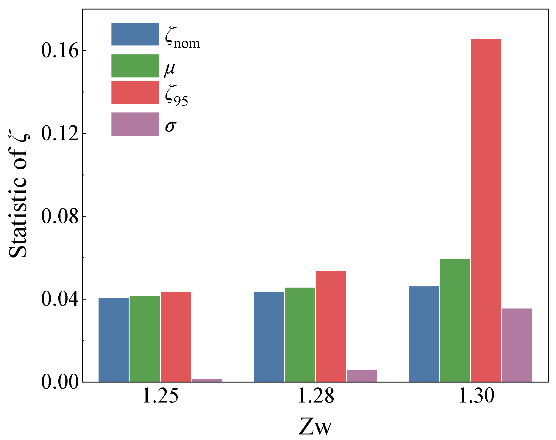
The above quantitative results show that as Zw increases from 1.25 to 1.30, the mean value and standard deviation of the loss increase sharply, whereas the nominal loss increases only slightly. The high-loss risk is also greatly amplified, as shown in Figure 9, where ζ₉₅ denotes the 95% percentile of ζ, and σ is plotted as the absolute standard deviation of ζ. At lower loading, the influence of actual manufacturing deviations is mainly reflected by a moderate increase in the loss level and its scatter. Under high-loading conditions, however, the aerodynamic performance of the low-pressure turbine becomes highly sensitive to small geometric deviations. The primary consequence of actual manufacturing deviations is then expressed as an amplified upper-tail loss risk, together with premature open separation for part of the manufactured geometries while the nominal geometry still remains in a weakly separated state. Therefore, a blade row that appears acceptable based on the nominal geometry may still contain a non-negligible fraction of high-loss manufactured geometries. In addition to the mean loss, statistical quantities such as the standard deviation, upper-tail quantiles, and high-loss event probabilities should be used to evaluate the aerodynamic effects of leading-edge deviations.

To examine whether the effect of the measured leading-edge deviations remains evident under off-design incidence conditions, additional calculations are performed at ±3° incidence for Zw = 1.28. The incidence range is selected because open suction-side separation begins to occur for the nominal geometry at approximately +4.5° to +5°, and +3° therefore represents a positive-incidence condition before this open separation occurs. As listed in

Table 3. Aerodynamic statistics of measured leading-edge deviation samples under different incidence conditions.

Incidence Angle (°)	ζnom	μ	σ/ζnom	Skewness	Kurtosis	P(Δζ/ζnom > 20%)	P(Δζ/ζnom > 30%)	Open-Separation Samples
−3	0.0427	0.0431	1.9%	0.9	2.2	0.22%	0.06%	0
0	0.0437	0.0459	14.2%	12.5	208.8	6.1%	2.9%	4 (0.2%)
+3	0.0520	0.0887	87.3%	14.4	307.4	56.8%	49.8%	489 (27.5%)

and shown in Figure 10, the negative-incidence case reduces both the nominal loss and the overall loss level of the measured-deviation set. The mean loss decreases to 0.0431, the relative standard deviation is reduced to 1.9%, and no open-separation sample is observed, indicating that the high-loss risk caused by measured leading-edge deviations is notably weakened. In contrast, the positive-incidence case greatly amplifies the aerodynamic sensitivity to the same measured deviations. The nominal loss increases to 0.0520, while the mean loss of the measured samples rises to 0.0887, with a relative standard deviation of 87.3%. Moreover, 56.8% and 49.8% of the samples show loss increases larger than 20% and 30%, respectively, and open suction-side separation occurs in 489 samples, corresponding to 27.5% of the database. This deterioration is much stronger than the loading increase from Zw = 1.28 to Zw = 1.30 at zero incidence, for which the mean loss is 0.0596 and the open-separation probability is 9.4%. These results indicate that positive incidence can significantly amplify the sensitivity of highly loaded LPT blades to measured leading-edge geometric deviations.

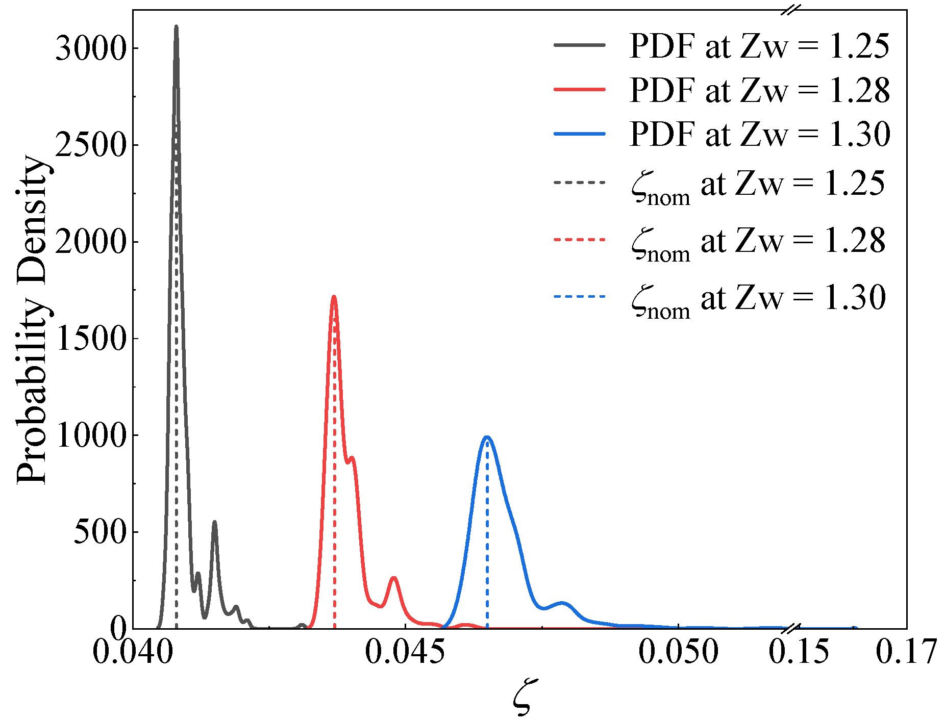
Apart from the effects of measured geometric deviations, the aerodynamic effects of the smooth GP-based leading-edge deviations are also given in Figure 11 and

Table 4. Aerodynamic statistics of GP-based leading-edge deviation samples under different loading levels.

Zw	ζnom	μ	σ/ζnom	Skewness	Kurtosis	P(Δζ/ζnom > 20%)	P(Δζ/ζnom > 30%)	Open-Separation Samples
1.25	0.0408	0.0409	0.8%	2.3	10.2	0	0	0
1.28	0.0437	0.0440	1.5%	8.3	114.2	0.25%	0	0
1.30	0.0465	0.0471	12.3%	19.5	385.3	0.25%	0.25%	1 (0.25%)

for comparison. The GP samples exhibit much narrower loss distributions than the measured-deviation samples. The mean loss remains close to the nominal value at all three loading levels, and the probabilities of a loss increase exceeding 20% or 30% are very small. Although the skewness and kurtosis of the GP results can be affected by a few rare outlying samples, the overall loss scatter and high-loss probability are far lower than those obtained from the measured deviations. This indicates that the present smooth GP model can represent part of the thickness-related response, but it does not reproduce the broad high-loss tail observed in the measured-deviation set. Therefore, for this database, using only a smooth GP deviation model may lead to a non-conservative evaluation of the upper-tail loss risk under high loading.

3.2. Thickness-Governed Loss Trend and Its Limitation

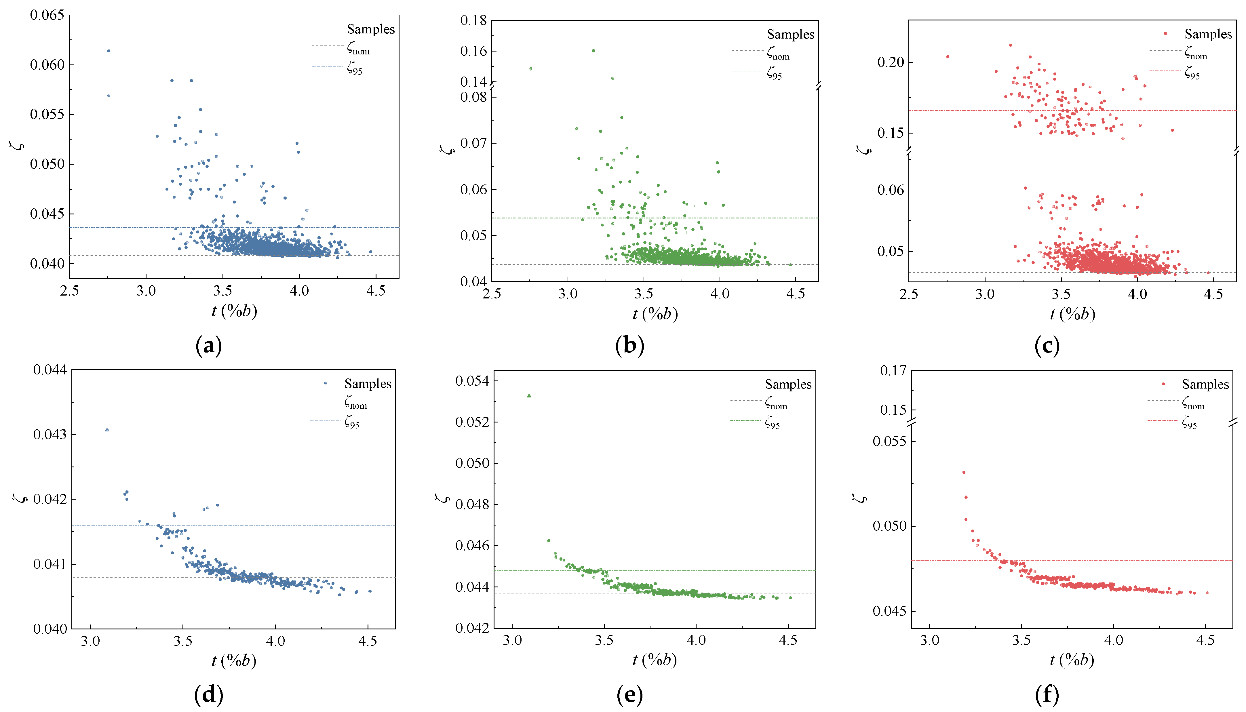
Based on existing studies, the leading-edge thickness has a significant impact [14,19,20], and its influence is first examined before more detailed measured-geometry effects are discussed. The loss coefficient ζ is plotted against the leading-edge thickness t for the measured-deviation samples in Figure 12a–c and for the smooth GP-based samples in Figure 12d–f.

For the measured samples, a clear thickness-related trend is observed. Samples with a thinner leading edge generally produce higher loss, whereas samples with a thicker leading edge tend to remain closer to the nominal loss level. This tendency becomes stronger as Zw is increased, and the high-loss tail is mainly formed on the thinner-leading-edge side. This indicates that leading-edge thickness acts as a first-order factor governing the loss variation.

The same analysis is performed for the smooth GP-based leading-edge deviation samples, and the results are given in Figure 12d–f. For the GP-based samples, the thickness-related trend is smoother and the vertical scatter is smaller, especially under higher loading. This trend is expected because smooth stochastic perturbations can still modify the local leading-edge scale, the suction-side acceleration, and the boundary-layer state. Representative GP samples with thin and thick leading edges, as well as the nominal blade profile, are used to analyse the mechanism by which thickness affects the flow field and performance. A comparison of leading-edge thickness and ζ is listed in

Table 5. Comparison of leading-edge thickness and ζ of three typical profile samples.

Profile	Leading-Edge Thickness	ζ at Zw = 1.20	ζ at Zw = 1.25	ζ at Zw = 1.28	ζ at Zw = 1.30
Nominal	3.80% b	0.0375	0.0408	0.0437	0.0465
Thicker	4.51% b	0.0375	0.0406	0.0435	0.0461
Thinner	3.09% b	0.0386	0.0431	0.0533	0.1621

. Because the GP perturbations are spatially smooth, this comparison mainly reflects the aerodynamic consequence of changing the local leading-edge scale, with limited interference from local non-smoothness or irregular curvature variation. The comparison therefore provides a useful reference for separating the first-order thickness effect from the additional measured-geometry effects discussed later.

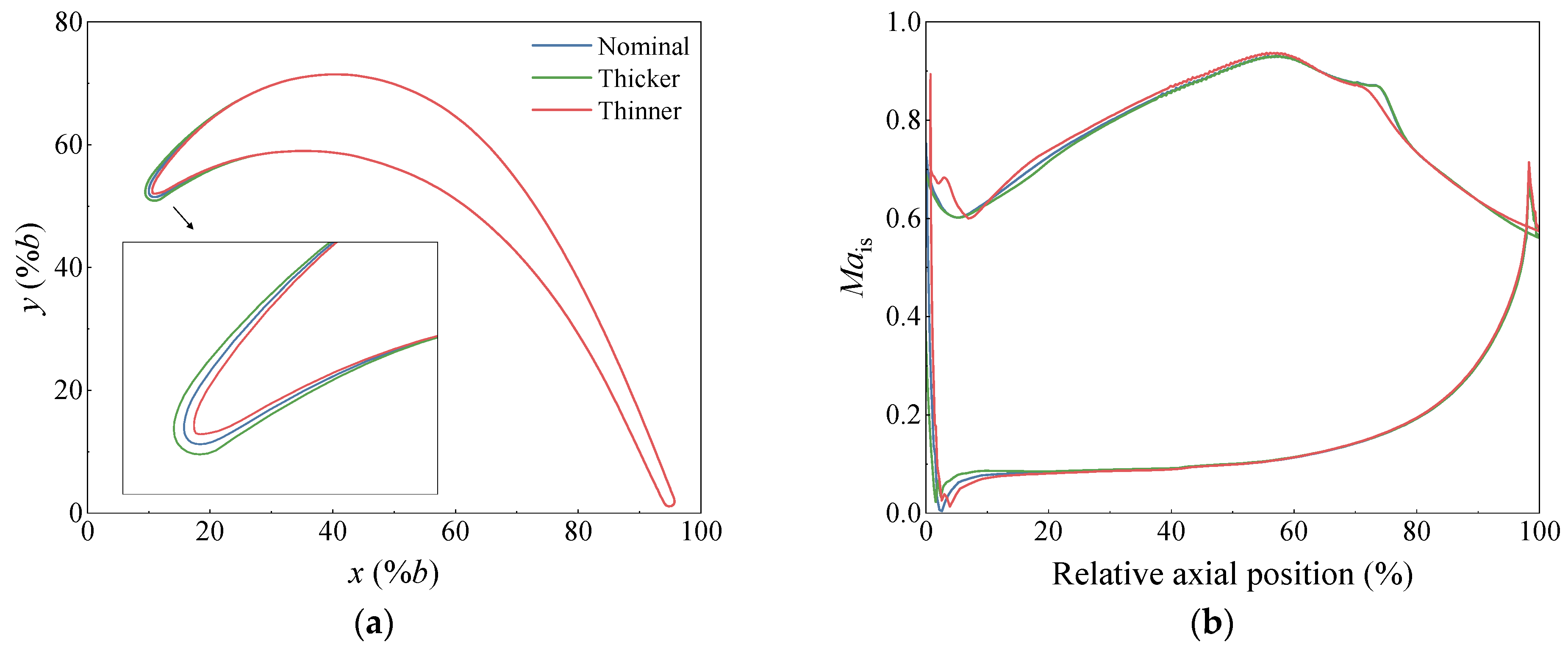
The comparison in Table 5 and Figure 13 is used to isolate the first-order effect of leading-edge thickness under smooth GP-based perturbations. The three profiles have different leading-edge scales but no notable local non-smoothness. Thus, the difference in their aerodynamic response is mainly related to the change in the leading-edge pressure-gradient development. The thinner leading edge forms a sharper front contour and a smaller local radius, whereas the thicker leading edge gives a blunter leading-edge region. 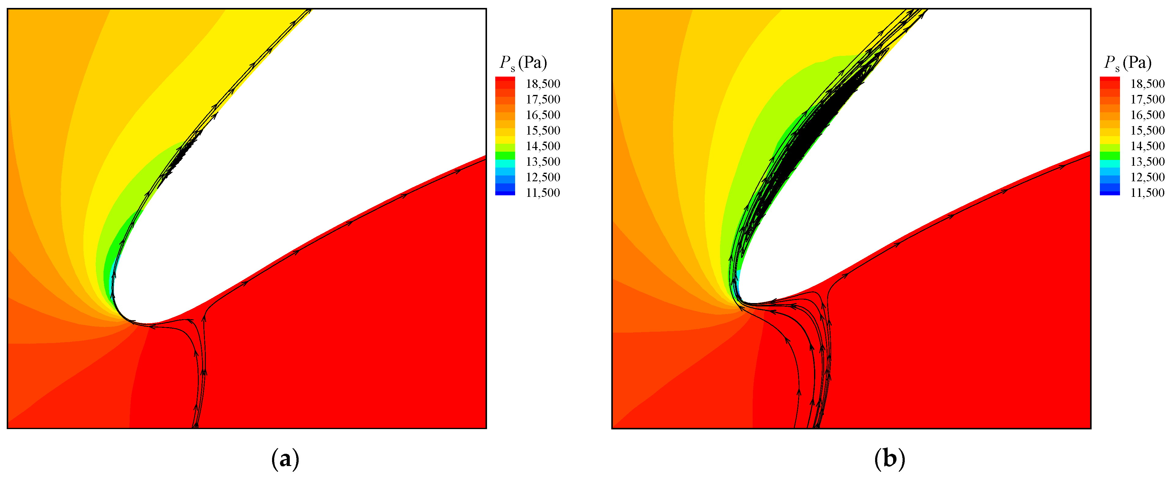As shown by the isentropic Mach number distribution in Figure 13b, the overall suction-side loading remains similar among the three cases. Clear differences are mainly observed near the suction-side leading edge. For these highly loaded LPT profiles, the near-leading-edge flow is deflected toward the suction side, as reflected by the streamline pattern and static-pressure field in Figure 14. The local acceleration is followed by a short adverse-pressure-gradient region. Under this condition, leading-edge thinning strengthens the suction-side pressure spike and produces a more abrupt pressure recovery immediately downstream. In contrast, leading-edge thickening slightly weakens the leading-edge response and gives a smoother initial acceleration.

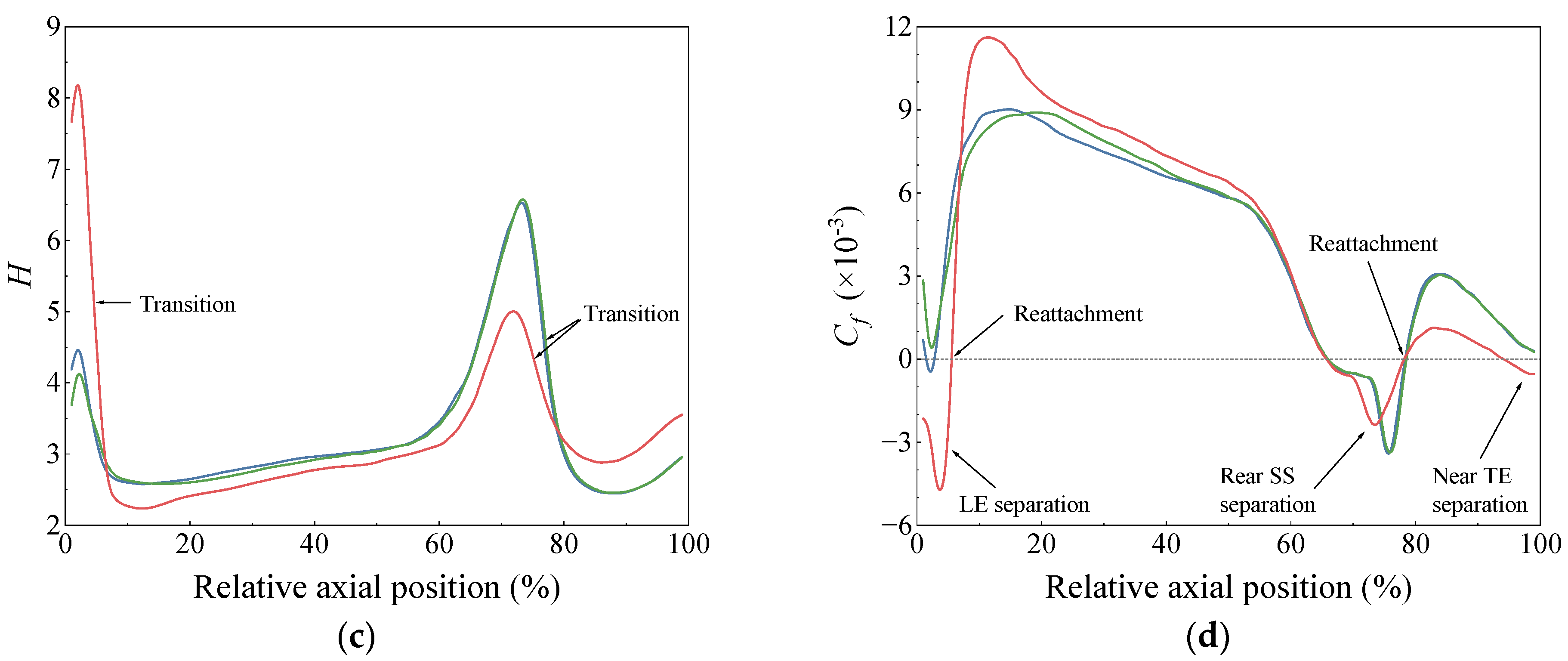
These local loading differences are reflected in the boundary-layer parameters on the suction side shown in Figure 13c,d. In Figure 13d, LE separation, rear SS separation, and near TE separation denote leading-edge separation, rear suction-side separation in the adverse-pressure region, and near-trailing-edge separation, respectively. For the thinner leading edge, the shape factor H has a higher peak near the leading edge, and the skin-friction coefficient C_f shows a negative region followed by a rapid recovery. These features indicate a stronger leading-edge separation bubble and a more pronounced separation-induced transition response near the front part of the suction side, as marked in Figure 13c. After reattachment, C_f remains at a higher level over the front and middle suction side. This indicates stronger wall-shear development over a longer streamwise distance so that more friction loss is accumulated before the rear adverse-pressure-gradient region is reached. For the nominal and thickened profiles, the leading-edge response is weaker. Their H peaks on the front suction side are lower, and the early skin-friction recovery is less abrupt. The main boundary-layer response is then more closely associated with the rear adverse-pressure-gradient region. This is shown by the downstream increase in H and the negative C_f region near the rear suction side. The marked transition-related locations indicate that the nominal and thickened profiles mainly show transition and recovery behaviour in the rear separated-flow region, whereas the thinner profile has already experienced a stronger leading-edge separation-induced transition. After this leading-edge separation bubble, the following acceleration region weakens the near-wall turbulent activity, so the rear transition-related response becomes less dominant for the thinner profile. Thus, leading-edge thinning changes not only the local pressure spike but also the downstream boundary-layer development.

The static-pressure fields and streamlines in Figure 14 provide further support for this interpretation. Compared with the nominal profile, the thinner leading edge produces a stronger low-pressure region near the suction-side leading edge and a clearer local separation response. This agrees with the higher leading-edge shape factor, the negative skin-friction region, and the earlier transition-related location shown in Figure 13c,d. The subsequent high skin-friction level over the front and middle suction side explains the larger accumulated loss of the thinner profile. When the flow enters the rear adverse-pressure-gradient region, the boundary layer has already been altered by the leading-edge separation and transition process. Therefore, the downstream recovery becomes less favourable, and the boundary layer before the trailing edge has lower momentum. This increases the wake-mixing loss and explains why the thinner profile gives a much larger loss at high loading and reaches large-scale open separation at Zw = 1.30.

The thickened leading edge shows the opposite tendency, but the improvement is limited. Its leading-edge pressure spike is slightly weakened, and the front-suction-side skin-friction level remains lower than that of the thinner case. The rear separation and recovery behaviour are also closer to the nominal condition. However, the downstream adverse-pressure-gradient region is still mainly determined by the overall cascade loading. As a result, the benefit from moderate thickening does not increase symmetrically with the penalty caused by thinning. This asymmetric response is consistent with the loss statistics in Figure 11 and Table 4. At low loading, the loss difference between the three representative profiles is small. As the loading is increased, the thinner leading edge produces a rapidly increasing loss penalty and triggers large-scale open separation at Zw = 1.30, whereas the thickened leading edge gives only a modest reduction in loss. Therefore, leading-edge thickness provides the first-order geometric trend of the loss variation, but this trend is strongly nonlinear under high loading.

The GP-based thickness comparison therefore provides two roles in the present analysis. First, it indicates that smooth leading-edge perturbations can capture the aerodynamic consequence of changing the local leading-edge scale since the variations in loading, shape factor, and skin friction follow the expected thinning and thickening trends. Second, it provides a reference for judging whether a measured profile produces a loss higher than that expected from thickness alone. If a measured sample has a leading-edge thickness comparable to a GP-based sample or another measured sample but still produces a much larger loss, the additional penalty should be related to local measured-geometry features rather than to the first-order thickness effect. In this sense, thickness is regarded as the background geometric scale, while local non-smoothness and irregular curvature variation are examined as additional sources of high-loss risk.

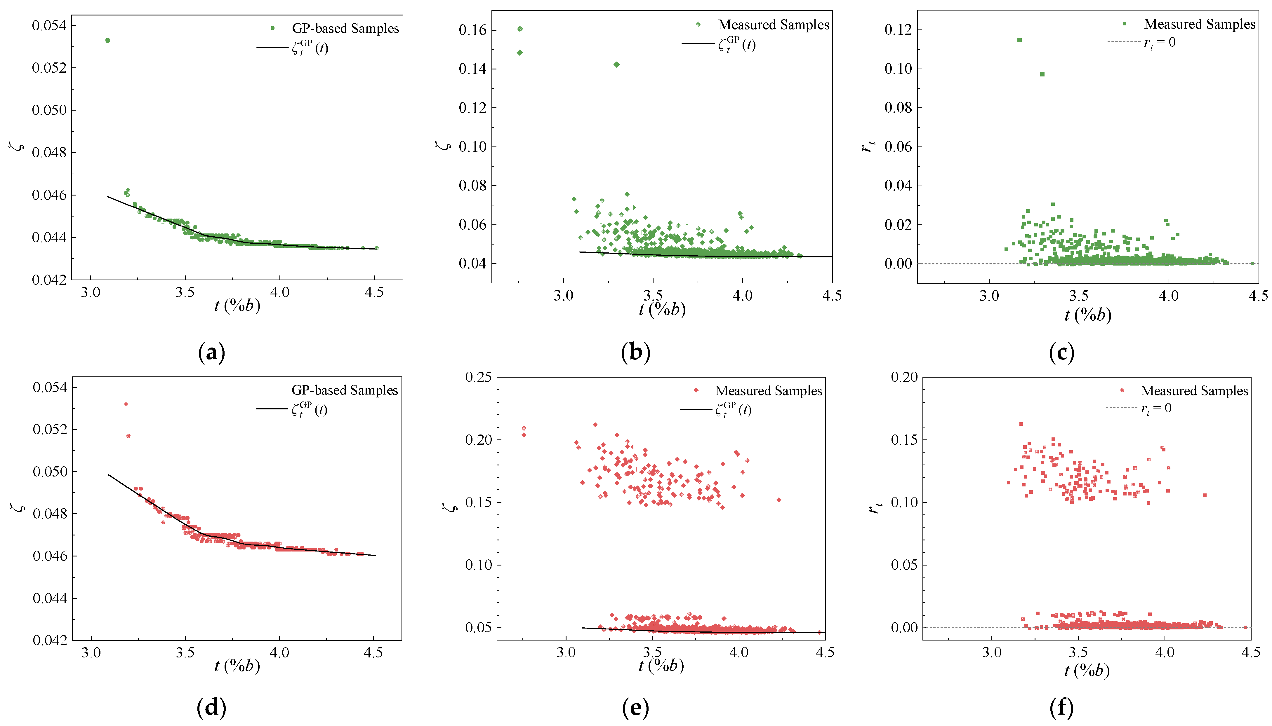
To separate the first-order thickness effect from the additional loss caused by measured local geometry, a smooth thickness baseline is defined from the GP-based deviation samples at Zw = 1.28 and 1.30. The same procedure can be applied at Zw = 1.25. Because the residual difference and high-loss risk are much weaker at this loading level, only Zw = 1.28 and 1.30 are shown in Figure 15 to focus on the high-loading amplification effect. The GP samples are used for this purpose because their leading-edge perturbations are spatially smooth and mainly reflect the change in local leading-edge scale. For each Zw, the relation between the leading-edge thickness t and loss coefficient ζ is fitted from the GP-based samples using robust locally weighted regression with tricube distance weighting and iterative bisquare reweighting. The fitted curve is denoted as ${\zeta }_{GP}^t$(t). The residual of each measured sample is then defined as r_t = ζ − ${\zeta }_{GP}^t$(t). A positive rt means that the measured geometry produces a loss higher than the value expected from the smooth thickness-controlled trend.

The thickness-conditioned ζ residuals are presented in Figure 15. Panels (a) and (d) show the GP-based thickness baseline at Zw = 1.28 and 1.30, respectively. Panels (b) and (e) place the measured samples against the same baseline, showing that many measured profiles lie far above the smooth thickness trend. Panels (c) and (f) present the corresponding residuals. The much wider positive-residual tail of the measured samples indicates that leading-edge thickness explains the primary trend but cannot account for the high-loss measured profiles. This residual behaviour gives the statistical motivation for the same-thickness comparison in Section 3.3, where the additional loss mechanism is examined using representative measured and GP-based profiles.

3.3. Additional Loss Induced by Measured Local Geometry Under Comparable Thickness

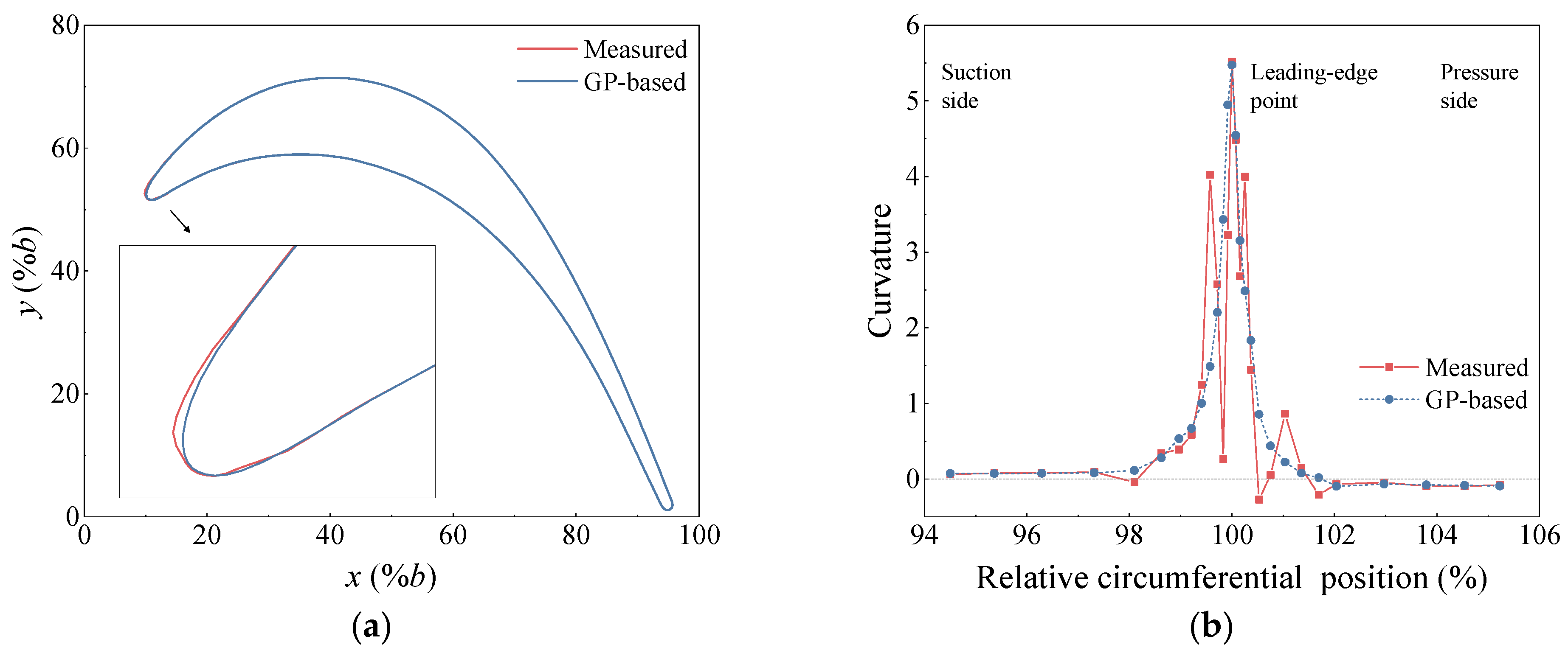
The above analysis indicates that the thickness effect is important but incomplete. To examine the loss component beyond thickness, one measured profile and one GP-based profile with the same leading-edge thickness of 3.67% b are selected. This pair allows the local shape effect to be compared under an approximately identical leading-edge scale. Their profiles and curvature distributions are shown in Figure 16. Although the two samples have the same thickness, the measured sample produces a much larger loss as the loading is increased, as listed in

Table 6. Comparison of leading-edge thickness and ζ of measured and GP-based samples.

Profile	Leading-Edge Thickness	ζ at Zw = 1.20	ζ at Zw = 1.25	ζ at Zw = 1.28	ζ at Zw = 1.30
Nominal	3.80% b	0.0375	0.0408	0.0437	0.0465
Measured	3.67% b	0.0382	0.0426	0.0526	0.1556
GP-based	3.67% b	0.0375	0.0409	0.0440	0.0469

. At Zw = 1.30, large-scale open separation already appears for the measured sample, whereas the GP-based sample still remains close to the nominal loss level. This comparison indicates that a local measured geometry other than thickness can still introduce a substantial additional loss.

The leading-edge comparison in Figure 16 shows that the difference between the two profiles is mainly associated with local shape regularity and curvature variation. The GP-based profile gives a smooth deformation along the leading-edge arc. Its curvature changes regularly from the suction-side leading-edge segment to the pressure-side leading-edge segment. By contrast, the measured profile contains a less regular leading-edge contour and a more nonmonotonic curvature distribution. Additional curvature extrema and local oscillations appear near the transition from the leading edge to the adjacent blade surfaces. These geometric features have small coordinate amplitudes, but they modify the curvature continuity experienced by the near-wall flow. For a highly loaded LPT blade, where the suction-side leading edge is already exposed to strong acceleration followed by an adverse pressure gradient, such local curvature-variation irregularities can change the local pressure-gradient continuity and make the early boundary-layer response more sensitive to the measured geometry.

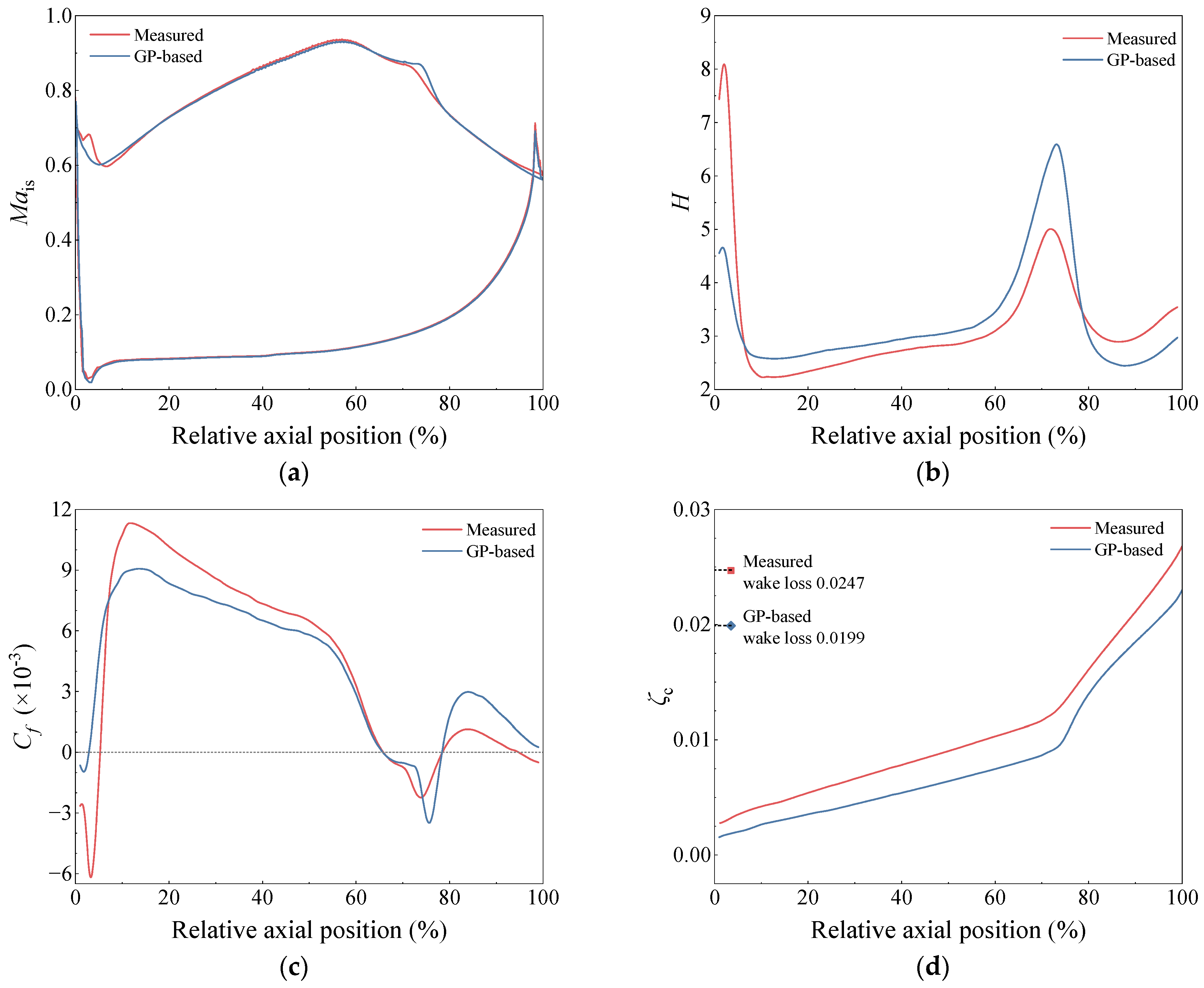
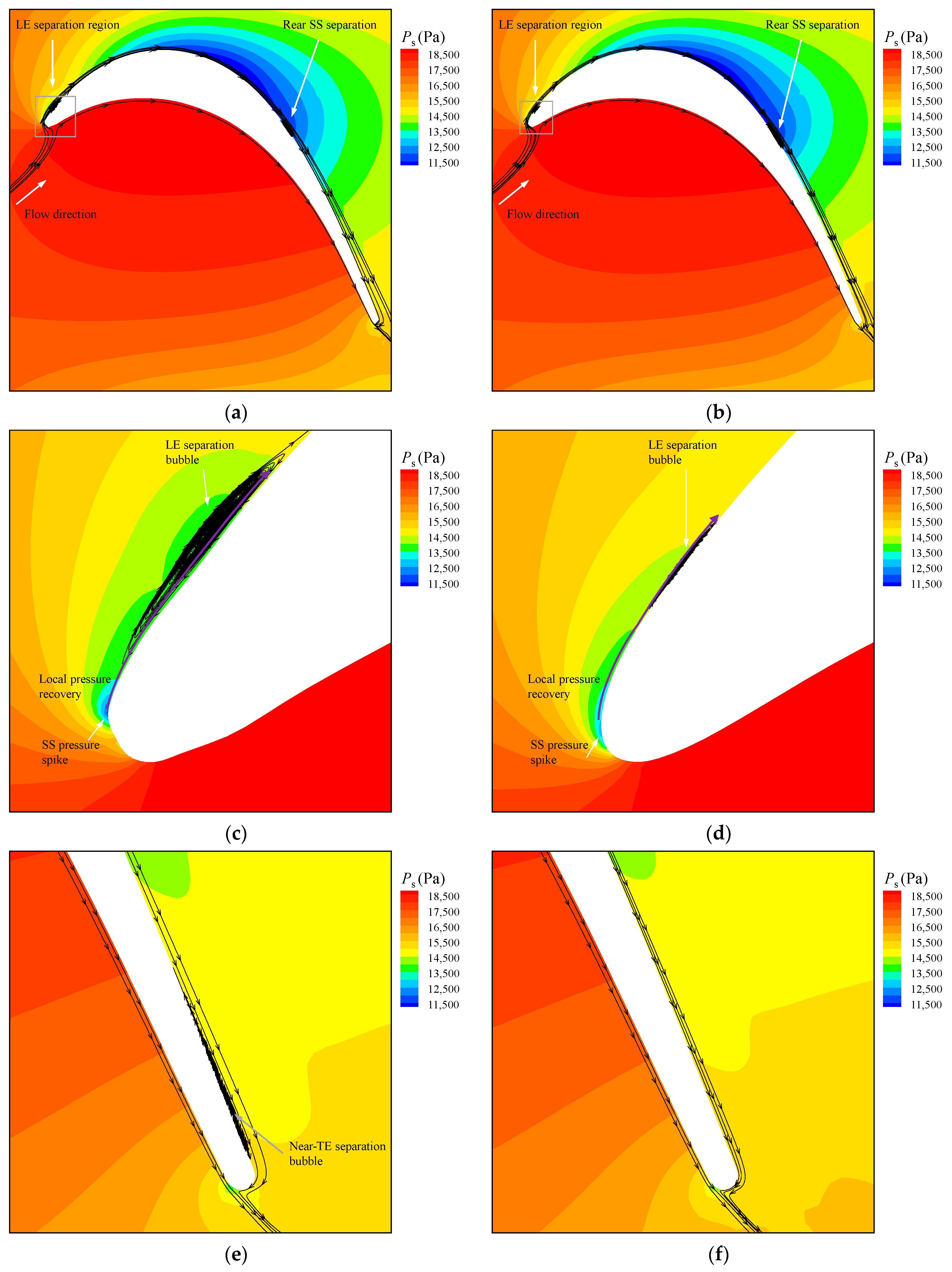
The flow parameters and static-pressure fields at Zw = 1.28 in Figure 17 and Figure 18 explain how this local geometric difference is converted into loss. Here, ζ_c denotes the cumulative total-pressure loss coefficient on the suction side from the leading edge to the current streamwise position, which is defined by Equation (4), where ρ, v_t, and P_t denote the local density, tangential velocity, and total pressure within the boundary layer, respectively; δ_bd is the local boundary-layer thickness, and ṁ is the passage mass flow rate per unit span used for normalization. The numerator represents the mass-flow-weighted total-pressure deficit within the local boundary layer. Therefore, ζ_c describes the streamwise development of the suction-side boundary-layer loss using the same pressure scale as the overall loss coefficient in Equation (1). The measured and GP-based profiles have similar overall loading over most of the blade surface. The main difference appears in the local pressure-gradient history near the suction-side leading edge and in the subsequent development of the suction-side boundary layer. For the measured profile, the less regular curvature variation strengthens the local pressure-gradient nonuniformity around the leading-edge pressure spike. This promotes earlier local separation and transition near the leading edge, producing a larger initial loss and modifying the boundary-layer state before the flow enters the middle suction-side region.

$${\mathsf{\zeta }}_{\mathrm{c}}\left(x\right)={\displaystyle \frac{{\displaystyle {\int }_0^{{\mathsf{\delta }}_{\mathrm{bd}}\left(x\right)}\rho v_{\mathrm{t}}\left(P_{\mathrm{ti}}-P_{\mathrm{t}}\right)\mathrm{d}y}}{\dot{m}\left(P_{\mathrm{to}}-P_{\mathrm{so}}\right)}}$$

(4)

The full-passage views and the local zoom-in plots in Figure 18 provide complementary evidence for this upstream-to-downstream effect. The LE zoom-in shows that the measured sample produces a stronger suction-side pressure spike, followed by a local pressure-recovery region and a clearer leading-edge separation bubble. This early disturbance is then reflected in the full-passage view by a more disturbed suction-side boundary-layer development downstream. A closed separation region is observed in the downstream adverse-pressure-gradient region, corresponding to the rear SS separation marked in Figure 18a. Further downstream, the near-TE zoom-in in Figure 18e shows that a thin separation bubble remains near the end of the suction side for the measured sample. For the GP-based sample, the leading-edge response is smoother and weaker. Although a separated-flow region is also present in the downstream adverse-pressure-gradient region, no comparable near-TE separation bubble is observed. Therefore, the larger loss of the measured sample is associated with the boundary-layer development imposed by the stronger leading-edge disturbance, rather than with the intensity of the separation in the downstream adverse-pressure-gradient region alone.

After this leading-edge response, the measured profile develops with a higher wall-shear level over the front and middle part of the suction side. This is reflected by the higher C_f level and the faster growth of ζ_c in Figure 17. Thus, the loss is accumulated as the disturbed boundary layer develops downstream. When the flow reaches the rear adverse-pressure-gradient region, the boundary-layer state has already been changed by the upstream leading-edge separation and transition process. This is reflected by the lower boundary-layer momentum and the larger shape factor H of the measured profile. Further downstream, the near-TE zoom-in in Figure 18e shows a thin separation bubble near the end of the suction side, whereas no comparable near-TE separation bubble is observed for the GP-based sample. This small near-TE separation bubble indicates that the downstream recovery of the measured profile remains less favourable, with lower boundary-layer momentum and a larger shape factor H. As the loading is increased to Zw = 1.30, this near-TE separation develops rapidly, extends upstream along the suction side, and finally forms large-scale open separation. This thicker and lower-momentum boundary layer strengthens the wake-mixing process [37], which is consistent with the larger wake loss shown in Figure 17d.

Figure 17 and Figure 18 therefore support one continuous mechanism. Local measured-geometry irregularity disturbs the leading-edge pressure-gradient development, modifies the suction-side boundary-layer state, increases cumulative friction loss over the front and middle suction side, weakens the rear suction-side recovery, and finally increases wake-mixing loss.

The loading comparison in Table 6 further confirms this amplification process. At Zw = 1.20 and 1.25, the adverse pressure gradient on the suction side is weaker, so the boundary layer can tolerate the leading-edge disturbance to a larger extent and the additional loss remains limited. At Zw = 1.28, the same local geometry difference produces a clear loss increase because the suction-side boundary layer becomes more sensitive to the leading-edge pressure-gradient disturbance and the subsequent downstream recovery. When Zw is further increased to 1.30, the rear suction-side boundary layer operates under a more severe adverse-pressure-gradient condition. The boundary-layer difference originating from the measured leading edge is then amplified rapidly, and the rear separation extends upstream into a large-scale separated state. The GP-based profile has the same leading-edge thickness, but its smoother local contour and more regular curvature variation produce a weaker leading-edge disturbance. Its downstream boundary-layer recovery is therefore better preserved, and its loss remains close to the nominal level.

The mechanism can be summarized from the perspective of upstream-to-downstream boundary-layer development. Leading-edge thickness determines the first-order scale of the local acceleration. Beyond the first-order thickness effect, measured local non-smoothness and irregular curvature variation alter the continuity of the near-wall pressure-gradient development at the leading edge. In a highly loaded LPT blade, this local loading disturbance changes the initial suction-side boundary-layer state. The disturbance is then amplified through local separation and transition, front-to-middle suction-side friction accumulation, rear adverse-pressure-gradient response, and wake mixing. Under moderately high loading, the consequence is mainly a larger loss scatter. Under higher loading, the same mechanism can produce a heavier high-loss tail and earlier large-scale suction-side separation.

This same-thickness comparison also clarifies the limitation of smooth GP-based perturbations. Such perturbations can reproduce the overall spatially correlated change in leading-edge geometry and can capture the thickness-related loss trend. However, the local non-smoothness and irregular curvature variation observed in measured profiles are not effectively represented by the smooth GP samples. These local features introduce additional pressure-gradient nonuniformity and make the suction-side boundary layer more sensitive to increasing loading. Therefore, for highly loaded LPT blades, leading-edge tolerance assessment should not rely only on thickness range or smooth random-field deviations. The regularity of the local leading-edge shape should also be considered when assessing deviation-induced high-loss risk.

The present results are generally consistent with previous studies showing that increased loading and positive incidence can amplify the aerodynamic sensitivity of turbine blades to geometric variations [15,16,17,18]. Earlier investigations have often focused on idealized or parametrically defined geometric changes, such as leading-edge radius, or smooth stochastic deviations based on a Gaussian process [8,12]. These studies have shown that leading-edge geometry can significantly affect suction-side acceleration, transition, separation, and profile loss. The present work further extends this understanding by using a large set of measured leading-edge deviations and by comparing them with a GP-based smooth stochastic reference. The comparison indicates that leading-edge thickness provides the major loss trend, while measured local non-smoothness and irregular curvature variation can introduce additional high-loss risk at the same thickness level. Therefore, the measured-deviation effect observed here is complementary to previous idealized or smooth-deviation studies and highlights the need to consider realistic local leading-edge regularity in tolerance assessments and robust blade design.

The present findings can be used to guide robust aerodynamic optimization of highly loaded LPT blades. In addition to reducing the nominal profile loss, the optimization objective should also include the reduction in loss sensitivity to measured leading-edge deviations, especially local non-smoothness and irregular curvature variation. Such robustness may be improved through both leading-edge geometry control and optimization of the whole profile. A suitable leading-edge thickness can help avoid an excessive suction-side pressure spike. Meanwhile, whole-profile optimization may provide additional freedom to moderate the suction-side loading and reduce the downstream amplification of leading-edge disturbances. This strategy is expected to reduce the probability of deviation-induced high loss and early open separation while maintaining low nominal loss.

4. Conclusions

The aerodynamic effects of measured leading-edge geometric deviations on a highly loaded LPT blade have been investigated. A set of 1781 measured leading-edge deviations is mapped onto the T106D-EIZ profile and compared with a GP-based smooth stochastic deviation model. The main conclusions are as follows.

(1)

Measured leading-edge geometric deviations produce a clear load-dependent increase in loss scatter and high-loss risk in the highly loaded LPT blade. At Zw = 1.28, the mean loss increases by 5.1% relative to the nominal value, and the relative standard deviation is 14.2%. The loss distribution is right-skewed, with a 2.9% probability of an increase exceeding 30%. When the loading is further increased to Zw = 1.30, open suction-side separation is triggered in approximately 9.4% of the measured profiles, and the probability of a loss increase exceeding 30% reaches 9.5%. These results show that the aerodynamic impact of realistic leading-edge deviations shifts from moderate loss scatter at lower loading to pronounced high-loss and premature-separation risks under higher loading.

(2)

Leading-edge thickness is identified as a major geometric factor contributing to the loss variation. Both the measured and GP-based deviation samples show that thinner leading edges generally produce higher loss, whereas thicker leading edges remain closer to the nominal performance. Flow analysis indicates that leading-edge thinning strengthens the local suction-side pressure spike and adverse pressure gradient, induces local separation and transition, increases downstream friction loss, and reduces the momentum within the boundary layer before the trailing edge. The aerodynamic penalty caused by thinning is therefore larger than the benefit obtained from moderate thickening, which explains the right-skewed loss distribution.

(3)

The same-thickness comparison further shows that measured local geometric irregularity can induce additional loss. In the representative same-thickness comparison, the measured sample reaches ζ = 0.1556 at Zw = 1.30, whereas the GP-based sample remains close to the nominal level with ζ = 0.0469. This difference is associated with local non-smoothness and irregular curvature variation in the measured leading edge. These features disturb the near-wall pressure-gradient development, modify the early suction-side boundary-layer state, and increase both cumulative suction-side loss and wake-mixing loss. These results indicate that realistic leading-edge shape quality should be considered in tolerance assessments and robust aerodynamic design of highly loaded LPT blades.

Several scope restrictions should be noted. The present conclusions are mainly derived from 2D midspan profile-loss analysis of leading-edge deviation patterns mapped onto the T106D-EIZ reference profile. Endwall effects, secondary flows, and spanwise-varying measured deviations are not included in the large-sample calculations. The 3D verification is limited to representative cases, and the off-design incidence analysis is conducted at Zw = 1.28 for two representative incidence angles. Broader 3D and off-design assessments should be considered in future work.