A TCN-FEP Hybrid Model with Multi-Scale Feature Interaction Network for Departure Runway Occupation Time Prediction

Abstract

Currently, improving runway utilization under operational safety constraints has become a critical concern for small and medium airports. Existing research focuses primarily on landing-phase runway occupation time, while predictive studies on the takeoff phase remain limited. Analysis of 1749 Quick Access Recorder (QAR) records from ten airports reveals that departure runway occupation time is strongly correlated with ground speed at liftoff (0.72) and airport elevation (0.67) but weakly correlated with aircraft weight and meteorological conditions, providing guidance for feature engineering. To address the prediction of departure runway occupation time, this study proposes a TCN-FEP hybrid model. The model employs an enhanced Temporal Convolutional Network (TCN) module with multi-scale convolutions (kernel sizes 3, 5, 7) and dilated convolutions (rates 2, 4, 8) to capture multi-scale feature interactions, alongside a Feature Enhancement Projection (FEP) module that maps local features into a high-dimensional latent space for implicit relationship mining and global information integration. Experimental results demonstrate that the proposed TCN-FEP model achieves an MSE of 90.20, RMSE of 9.49, MAE of 5.84 s, MAPE of 3.80%, and R² of 0.97, outperforming Informer (MSE 117.95), Longformer (MSE 132.11), XGBoost (MSE 92.30), and LightGBM (MSE 91.45). Under 5% outlier injection, MSE increases by 7.9%, compared to 24.3% for LSTM and 18.4% for Informer. With 94% of prediction errors within ±5 s, the model’s accuracy may offer a useful reference for runway resource optimization at small and medium airports.

1. Introduction

As of the end of 2025, small and medium-sized airports in China account for over 80% of the total number of transport airports. Most of these airports operate with a single runway and feature a simple runway–taxiway configuration. When operating in a specific direction, the majority of these airports require aircraft to perform a runway turn before takeoff or after landing. The time aircraft spend taxiing on runways and taxiways far exceeds air traffic control separation intervals and wake turbulence separation requirements, making it the primary factor limiting runway capacity at small and medium-sized airports. Therefore, the Departure Runway Occupation Time (DROT) serves as a key indicator for assessing runway operational efficiency, and its accurate prediction holds significant value for optimizing airport operational capacity [1]. Existing research has primarily focused on runway occupation time during the landing phase, with limited studies dedicated to predicting it during the takeoff phase. In actual operations, however, take-off and landing are interrelated and mutually influential, jointly determining overall runway efficiency. According to SESAR research [2], runway capacity is largely constrained by runway occupation time, a parameter influenced by multiple factors, including taxi route design, meteorological conditions, runway status, and aircraft type. In this context, constructing an accurate prediction model for departure runway occupation time based on airport operational characteristic data is of great importance for enhancing operational efficiency.

In recent years, researchers worldwide have explored the optimization of airport operational efficiency and runway capacity. In terms of model optimization, Xie Yubing et al. [3] employed a GA-PSO hybrid optimization for BP neural networks, significantly improving prediction accuracy. Liu Tao et al. [4] applied feedforward neural networks to runway capacity assessment, establishing a direct link between prediction results and operational efficiency. Pan Weijun et al. [5] integrated runway radar surveillance data, achieving an 8% improvement in BP neural network prediction accuracy. In recent years, with the advancement of machine learning techniques, Zhang Kexin et al. [6] proposed a KPCA-IWOA-ELM model that limits prediction errors to within 5%. Gu Runping et al. [7] developed a classification prediction model based on BP neural networks, effectively addressing the impact of aircraft type variations. Li Nan et al. [8] introduced a prediction model combining the grey wolf optimizer and random forest algorithm, achieving a prediction accuracy of 92% during peak flight operation periods—an improvement of approximately 15% over traditional random forest models. Chen Yaqing et al. [9] developed the SSA-CNN model, which, through intelligent optimization algorithms, not only adapts to different runway–taxiway configurations but also increases runway utilization at Shanghai Pudong International Airport by 12%. Internationally, Stamatopoulos et al. [10] developed an aviation decision support system, which, in real-world operational tests, was shown to accurately predict runway occupation duration. Ghalebsaz Jeddi et al. [11] conducted statistical analyses of runway usage data at Detroit Metropolitan Airport, finding that the probability distribution of runway occupation time more closely follows a mixed beta distribution. Gao et al. [12] constructed a prediction model for aircraft arrival runway occupation time (ROT) using machine learning techniques, enabling the model to automatically learn nonlinear relationships between ROT and multiple variables, outperforming traditional statistical methods. Nikoleris et al. [13] demonstrated through the development of a recursive queuing model that accurate prediction of runway occupation time is critical to improving four-dimensional trajectory precision. These studies have progressively advanced from theoretical approaches to engineering applications, collectively driving the development of runway occupation time prediction technologies toward higher accuracy and greater adaptability.

In parallel with the aviation-specific studies reviewed above, the broader machine learning community has made substantial progress in tabular data modeling—the category to which departure runway occupation time (DROT) prediction belongs. Unlike images or text, tabular data lacks explicit spatial or temporal structure, presenting unique challenges for deep neural networks. Traditional tree-based ensemble methods have long been considered the gold standard for tabular tasks due to their efficiency and robustness. Chen and Guestrin [14] proposed XGBoost, a scalable tree boosting system that incorporates regularization to prevent overfitting, achieving competitive results across numerous competition benchmarks. Ke et al. [15] introduced LightGBM, which employs gradient-based one-sided sampling (GOSS) and exclusive feature bundling (EFB) to dramatically reduce training time while maintaining accuracy. These methods, however, rely on feature engineering and lack the end-to-end representation learning capability of neural networks.

Recent deep learning architectures have begun to close the performance gap with tree-based methods on tabular data. Arik and Pfister [16] proposed TabNet, a canonical tabular learning architecture that employs sequential attention to select salient features at each decision step. TabNet’s design enables interpretable feature attributions and efficient learning by focusing computational capacity on the most relevant features, and further incorporates self-supervised pretraining to leverage abundant unlabeled data—a particularly valuable capability in aviation scenarios where labeled QAR data are expensive to annotate, but unlabeled recordings are plentiful. Popov et al. [17] developed Neural Oblivious Decision Ensembles (NODE), which bridges neural networks and decision trees by introducing a differentiable oblivious decision tree layer that enables end-to-end gradient-based optimization while preserving the inductive bias of tree ensembles. Gorishniy et al. [18] conducted a systematic revisit of deep learning for tabular data, proposing Feature Tokenizer Transformer (FT-Transformer) that treats each feature as a separate token and applies transformer attention across features. They demonstrated that FT-Transformer achieves competitive performance with proper regularization, establishing a strong baseline for attention-based tabular learning.

Beyond tabular-specific architectures, temporal sequence modeling methods also inform our approach, as DROT emerges from a sequential process (taxi → hold → takeoff roll). Bai et al. [19] proposed Temporal Convolutional Networks (TCN), demonstrating that convolutional architectures with causal and dilated convolutions can effectively capture long-range dependencies while enabling parallel training, outperforming recurrent networks on various sequence modeling benchmarks. Zhou et al. [20] introduced Informer, which addresses the quadratic complexity of Transformer on long sequences through ProbSparse attention and self-attention distilling, achieving significant improvements in long-term time series forecasting. Wu et al. [21] proposed Autoformer, which incorporates series decomposition and auto-correlation mechanisms to enhance the Transformer’s ability to capture seasonal-trend patterns.

While these advances provide valuable building blocks, none directly address the specific characteristics of DROT prediction: moderate feature dimensionality (9 dimensions), features originating from different phases of the departure process (taxi, hold, takeoff roll), and the need for robust generalization under real-world operational noise. It is worth noting that although DROT fundamentally follows physical laws such as kinematics and aircraft performance, idealized physical models (e.g., constant acceleration assumptions) struggle in practice to capture the complex nonlinear interactions among factors such as altitude, wind conditions, and pilot operating procedures. This is precisely where data-driven AI methods can provide value—not by replacing physical laws but by learning residual patterns from large amounts of real-world operational data to compensate for the limitations of purely physical models in complex environments. Based on this understanding, this study proposes a hybrid architecture that combines TCN’s capability for capturing local interactions (through multi-scale convolutions along the feature dimension) with a lightweight feature enhancement projection module. Unlike TabNet’s sequential attention, which is designed for high-dimensional tabular data, our projection module efficiently maps local features to a high-dimensional latent space without introducing quadratic complexity. The model first captures local feature variations at multiple scales through an enhanced TCN module, employing multi-scale convolutional kernels (sizes 3, 5, and 7) and a dilated convolution strategy (dilation rates 2, 4, and 8) to effectively extract multi-grained feature interactions during the departure phase. Subsequently, the model introduces a Feature Enhancement Projection (FEP) layer that maps the extracted local features into a high-dimensional latent space, enabling deep exploration of implicit correlations among features and global integration of key semantic information, thereby enhancing the model’s comprehensive representation capability for complex departure scenarios. This design reflects a fusion of artificial intelligence and traditional aviation engineering: physical models provide an interpretable foundational framework (such as the purely kinematic baseline we introduced), while deep learning models improve prediction accuracy by learning nonlinear residual patterns from data—the two are complementary rather than adversarial.

The practical implications of this research are threefold. First, the proposed model can be integrated into tower control automation systems to provide real-time DROT predictions, enabling controllers to optimize departure separation intervals. Second, the model supports scenario simulation: by inputting different meteorological and taxiing conditions, operators can anticipate runway occupancy under various operational scenarios. Third, the model facilitates runway capacity assessment based on historical prediction results, helping airports identify peak-hour congestion patterns and adjust flight release strategies accordingly. These applications collectively contribute to improved runway utilization at small and medium airports.

2. Analysis of Factors Influencing Departure Runway Occupation Time

The Quick Access Recorder (QAR), as an advanced flight data recording device, is capable of storing over 600 h of flight parameters, including critical flight indicators such as aircraft weight, airspeed, fuel status, and meteorological conditions [22]. Compared to conventional surveillance systems, which suffer from limitations such as large sampling intervals and incomplete data, the QAR system collects data at a sampling frequency of 1 Hz, offering advantages in terms of high data integrity and low missing rates. Utilizing QAR data enables a more accurate analysis of the entire aircraft process from takeoff to runway vacating, thereby providing a reliable data foundation for prediction research on departure runway occupation time.

2.1. Data Processing

To achieve accurate prediction of departure runway occupation time (DROT) at small and medium-sized airports, this study follows the standardized definition specified in the International Civil Aviation Organization (ICAO) Air Traffic Management Manual [23]. DROT is defined as the time interval from the moment the aircraft’s nose crosses the runway holding line until the main landing gear completely lifts off the runway surface.

Based on this definition, data preprocessing was conducted on 1749 departure QAR records provided by the airline.

(1)

Data Cleaning and Outlier Treatment: Missing values were filled using multiple imputation. For outlier detection, we adopted an airport-wise rather than global strategy, recognizing that values considered outliers at one airport may represent normal operating conditions at another. Specifically, for each airport, the interquartile range (IQR) method was applied to each feature. Flagged samples were then examined manually and corrected using multiple imputation rather than direct deletion, preserving maximum valid information. After removing missing, anomalous, duplicate, and invalid data, 1745 valid samples were obtained from the original 1749 records, yielding a data validity rate of 99%.

(2)

Feature Engineering: First, aircraft type information was converted into specific weight parameters to quantify weight variations during the departure phase. Second, to account for differences in runway configurations at small and medium-sized airports, a classification coding strategy for departure airports was adopted to construct feature variables encompassing dimensions such as the number of runways and layout configuration, effectively capturing the impact of the airport’s physical environment on DROT. Finally, the integration of multi-airport data enabled the model to be trained across operational scenarios with varying altitudes and taxiway configurations, thereby enhancing model adaptability in complex small and medium-sized airport environments.

(3)

Influencing Factor Extraction: Nine categories of influencing factors were extracted, including airport elevation, runway holding time before takeoff, ground speed at liftoff, departure runway, wind direction, wind speed, takeoff gross weight, distance from the taxiway intersection to the runway threshold, and whether a 180° turn was performed at the runway end during takeoff.

(4)

Data Source and Multi-Airport Aggregation: The QAR data were collected from ten small and medium-sized airports in Southwest China, operated by the cooperating airline. These airports span elevations ranging from 67.7 m to 849.4 m and feature various runway–taxiway configurations, including different runway lengths, intersection taxiway distances, and turn-back requirements.

Table 1. Processed QAR (Quick Access Recorder) data.

Airport	Elevation/m	DROT/s	V_LOF/kt	Runway	WD	WS/kt	TOW/lb	Distance/m	Whether to Turn Back
A	67.7	82	157	19	122	1	138,600	0	0
B	325	177	166	19	186	2	141,760	1168	1
C	100	126	164	31	186	4	150,080	0	0
D	820.4	219	159	13	107	7	134,120	0	1
E	727	234	171	1	196	1	143,200	0	1

presents representative samples from five different airports (A–E) to illustrate the data diversity.

The integration of multi-airport data into a single dataset is a deliberate choice, which can be justified from the following perspectives. First, airport elevation is explicitly included as an input feature, allowing the model to learn elevation-dependent patterns rather than treating elevation as a batch effect. Second, the diversity of operational scenarios across airports enhances model generalization, enabling the trained model to perform robustly at new airports without retraining. Third, small and medium airports often share similar operational characteristics (e.g., single runway, simple taxiway configuration), making cross-airport learning feasible. Nevertheless, to account for potential data heterogeneity, we employ airport-wise outlier detection and normalization (see Data Cleaning below) and include airport elevation as a key feature to control for airport-specific effects.

A sample of the normalized QAR data is presented in Table 1. The resulting structured feature system provides a high-quality data foundation for subsequent deep training of the TCN-FEP hybrid model.

2.2. Correlation Analysis

Correlation analysis is a statistical method used to quantify the degree of linear association between two or more variables, revealing the coordinated patterns of variation among variables through mathematical computation. Following preprocessing procedures such as data cleaning and feature engineering, conducting correlation analysis enables the quantification of the degree of association between each feature and the departure runway occupation time, facilitates the selection of key influencing factors, and eliminates redundant features, thereby reducing model complexity and mitigating the risk of overfitting.

2.2.1. Regression Analysis

The Pearson correlation coefficient is a commonly used statistical indicator for measuring the degree of linear association between two continuous variables [24]. The value of this coefficient ranges from −1 to 1, where an absolute value closer to 1 indicates a stronger linear correlation. The relevant calculation formula is as follows:

$$r={\displaystyle \frac{{\displaystyle {\sum }_{i=1}^n\left(x_i-\overline{x}\right)\left(y_i-\overline{y}\right)}}{\sqrt{{\displaystyle {\sum }_{i=1}^n{\left(x_i-\overline{x}\right)}^2{\displaystyle {\sum }_{i=1}^n{\left(y_i-\overline{y}\right)}^2}}}}}$$

(1)

$$\stackrel{\_}{x}={\displaystyle \frac{1}{n}}{\displaystyle {\sum }_{i=1}^n{x}_i}$$

(2)

$$\stackrel{\_}{y}={\displaystyle \frac{1}{n}}{\displaystyle {\sum }_{i=1}^n{y}_i}$$

(3)

In Equations (1)–(3), $x_i$ represents the independent variable samples, $y_i$ represents the dependent variable samples, $\overline{x}$ denotes the sample mean of the independent variable, $\overline{y}$ denotes the sample mean of the dependent variable, and $n$ is the number of samples.

2.2.2. Correlation Results Analysis

Based on the calculated correlation coefficients, the correlations between each factor and the departure runway occupation time are presented in

Table 2. The correlation between various factors and the Departure runway occupation time.

Factor	Correlation Coefficient with DROT
TOW	0.11
Elevation	0.67
Whether to turn back	0.43
WS	−0.29
V_LOF	0.72
Distance	0.48
Runway	−0.22
WD	0.02

.

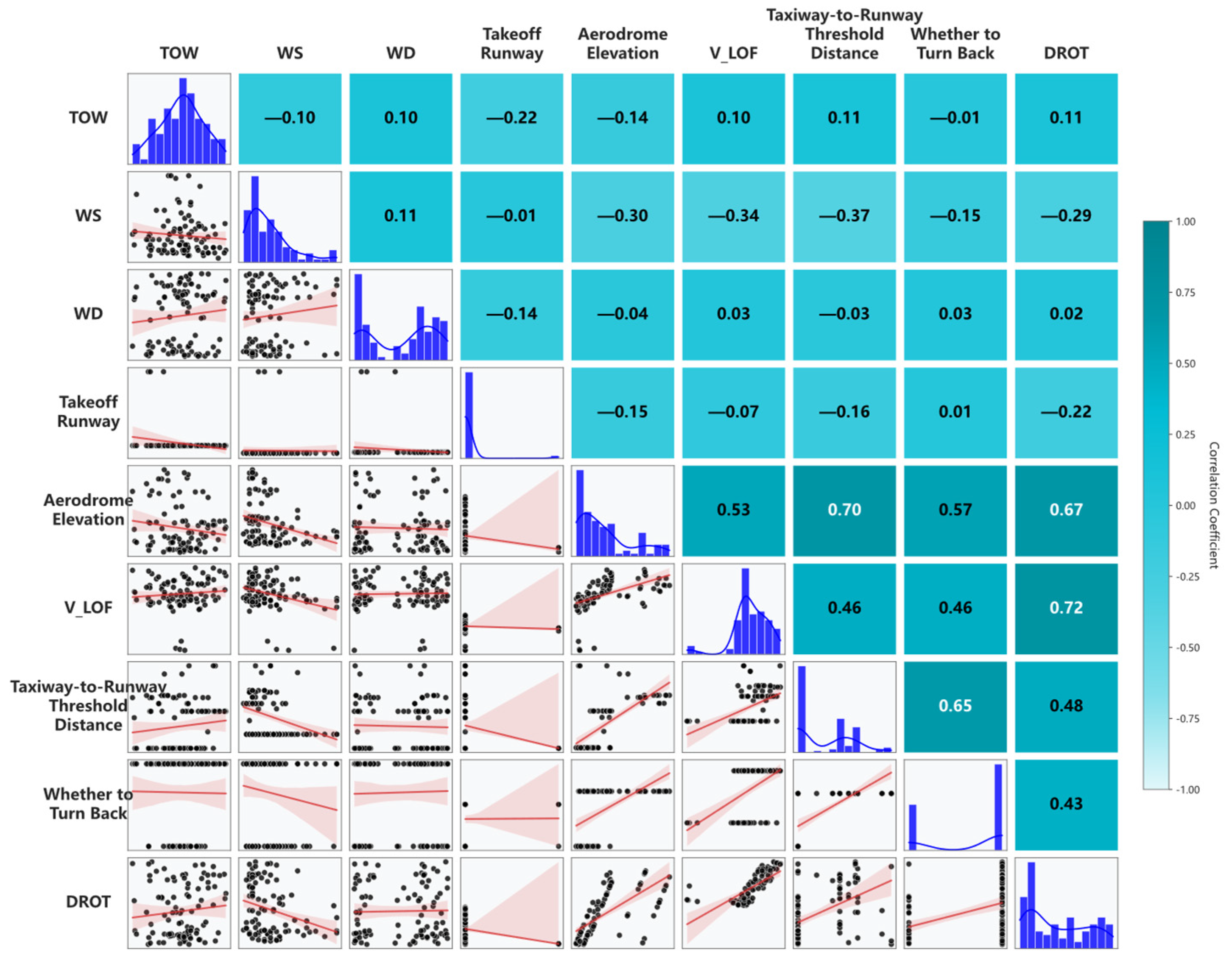
Based on the correlation coefficients, the core variables are identified as ground speed at liftoff and airport elevation. The correlation coefficient between ground speed at liftoff and departure runway occupation time reaches 0.72, indicating a strong positive correlation; that is, as ground speed at liftoff increases, departure runway occupation time is likely to increase. Airport elevation has a correlation coefficient of 0.67, also indicating a strong positive correlation: the higher the airport elevation, the longer the departure runway occupation time tends to be. In contrast, takeoff weight, wind speed, departure runway, and wind direction exhibit weak correlations with departure runway occupation time. Although the variables of whether a 180° turn is performed and the distance from the taxiway intersection to the runway threshold show some degree of correlation, their correlation strengths are relatively weaker compared to ground speed at liftoff and airport elevation.

To visually illustrate the degree of linear association between the key influencing factors and departure runway occupation time (DROT), a multivariate relationship matrix plot was constructed based on the standardized QAR data, as shown in Figure 1.

It is important to note that Pearson correlation measures linear association, not causation. While V_LOF and elevation show strong correlations with DROT, this does not imply that manipulating these variables would directly cause proportional changes in DROT. For instance, higher elevation often co-occurs with longer runways or modified takeoff procedures, which may be the actual causal factors. Correlation analysis serves here as a feature screening tool for the predictive model, not as a causal discovery method.

3. Construction of a TCN-FEP Hybrid Model for Predicting Takeoff Runway Occupation Time

3.1. Temporal Convolutional Network (TCN) Model

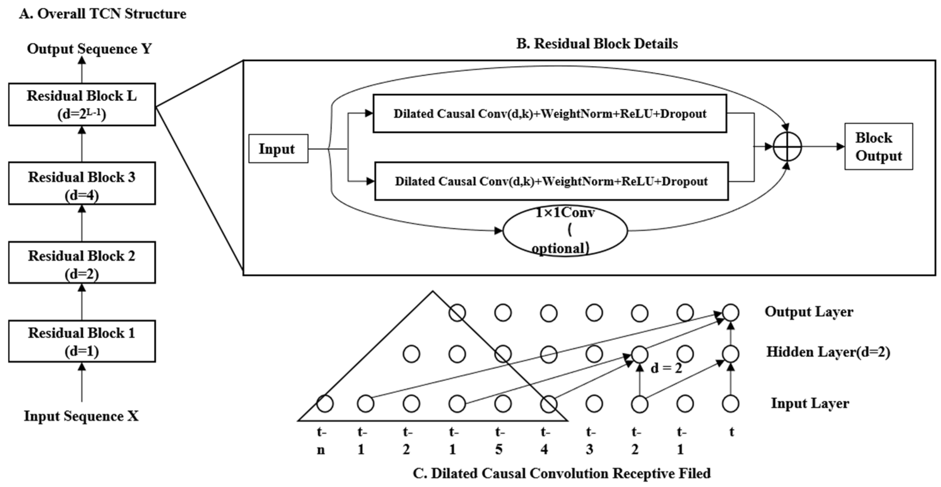
The Temporal Convolutional Network (TCN) [25] is a deep learning architecture specifically designed for sequence data modeling. Its core concept lies in replacing traditional recurrent structures with convolutional operations to address the inherent issues of Recurrent Neural Networks (RNNs) [26] and Long Short-Term Memory (LSTM) networks [27] regarding training efficiency and gradient stability. The design of TCN revolves around three key components. First, causal convolution ensures that the model strictly adheres to temporal causality, such that the prediction at time T depends only on historical information up to time T, thereby preventing future information leakage. Second, dilated convolution expands the receptive field in an exponential manner, enabling the network to capture long-range temporal dependencies without substantially increasing the number of parameters. Finally, the introduction of residual connections effectively alleviates the vanishing gradient problem in deep network training, ensuring stable gradient propagation across multiple layers.

This architectural design endows TCN with exceptional parallel computing capability—it can process an entire sequence in a single pass, enabling efficient training on GPUs while avoiding the gradient explosion or vanishing issues commonly encountered in RNNs. Furthermore, the size of its receptive field can be flexibly configured through network depth, kernel size, and dilation rate, rendering model behavior more controllable. However, TCN also has theoretical limitations imposed by its fixed receptive field: when the input sequence length exceeds the preset receptive field, it cannot capture the most distant historical information, and the number of parameters may increase in very deep networks. Therefore, TCN is particularly well-suited for scenarios where sequence lengths are moderate and fixed, with high requirements for real-time performance and rapid training, such as industrial control, speech synthesis, and financial forecasting, providing an efficient, stable, and powerful modeling paradigm for time series analysis. The specific architecture is illustrated in the Figure 2.

A clarification is necessary regarding our use of TCN. In this study, each input is a static feature vector from a single takeoff event, not a temporal sequence. We repurpose the TCN architecture by treating feature dimensions as positions in a 1D sequence and applying convolutions along this feature axis. Thus, what we refer to as “multi-scale feature interactions” in this paper means interactions among different subsets of features (e.g., between airport elevation and ground speed), rather than temporal dependencies across time steps. This reinterpretation enables the application of TCN’s powerful local feature extraction to tabular data. Causal padding is used to enforce a directional dependency in the feature sequence: the representation of each feature is computed only from itself and preceding features. This is consistent with the causal logic of the departure process, where certain features (e.g., takeoff weight) influence outcomes (e.g., ground speed) but not vice versa.

3.2. TCN-FEP Hybrid Model

Before presenting the model architecture, we justify why a deep learning approach is necessary for DROT prediction, despite the availability of simpler methods such as linear regression, ARIMA [28], or tree-based models (XGBoost, LightGBM). Three specific challenges motivate a more flexible architecture. First, DROT involves nonlinear feature interactions that additive models cannot fully capture. For example, the effect of wind speed on takeoff roll depends on both airport elevation and aircraft type. Neural networks can learn continuous representations of such conditional dependencies. Second, real-world QAR data contain noise and outliers from sensor errors and atypical operations. The multi-scale convolutional design helps average out local noise, while the high-dimensional projection reduces sensitivity to individual anomalous samples. Third, beyond point prediction, the features learned by TCN-FEP can be reused for downstream tasks such as anomaly detection, which tree-based models do not directly support.

These advantages motivate the hybrid TCN-FEP architecture, which combines an enhanced TCN module for local feature extraction with a lightweight Feature Enhancement Projection (FEP) layer for implicit relationship mining. The TCN-FEP hybrid model proposed in this study consists of three core modules.

• Enhanced TCN Feature Extraction Module

The enhanced TCN module adopts a multi-scale parallel one-dimensional causal convolutional network design with three scales. Specifically, three parallel convolutional layers are used, with kernel sizes of 3, 5, and 7, and dilation rates of 2, 4, and 8, respectively. Each convolutional layer has 64 output channels. The causal padding for each scale is computed as dilation × (kernel_size − 1) to ensure that the representation of each feature depends only on itself and preceding features, consistent with the causal logic of the departure process. Each convolutional layer is followed by a ReLU activation function and Dropout regularization (0.1) to prevent overfitting and enhance model generalization. Adaptive global average pooling is then applied to compress the features of each scale into a 64-dimensional vector. The features from the three scales are concatenated along the feature dimension, resulting in a fused feature vector of 192 dimensions. This provides a compact yet rich local representation for subsequent feature enhancement.

2.

Feature Enhancement Projection (FEP) within TCN-FEP

Within the complete TCN-FEP model, we introduce a lightweight Feature Enhancement Projection (FEP) layer that maps the 64-dimensional TCN output to a 128-dimensional latent space. This layer—consisting of 64 → 128 (ReLU, Dropout) → 128—enhances feature representation by uncovering nonlinear interactions among TCN-extracted local patterns. Note that the FEP is an internal component of the proposed model, not a standalone architecture.

3.

Regression Prediction Head

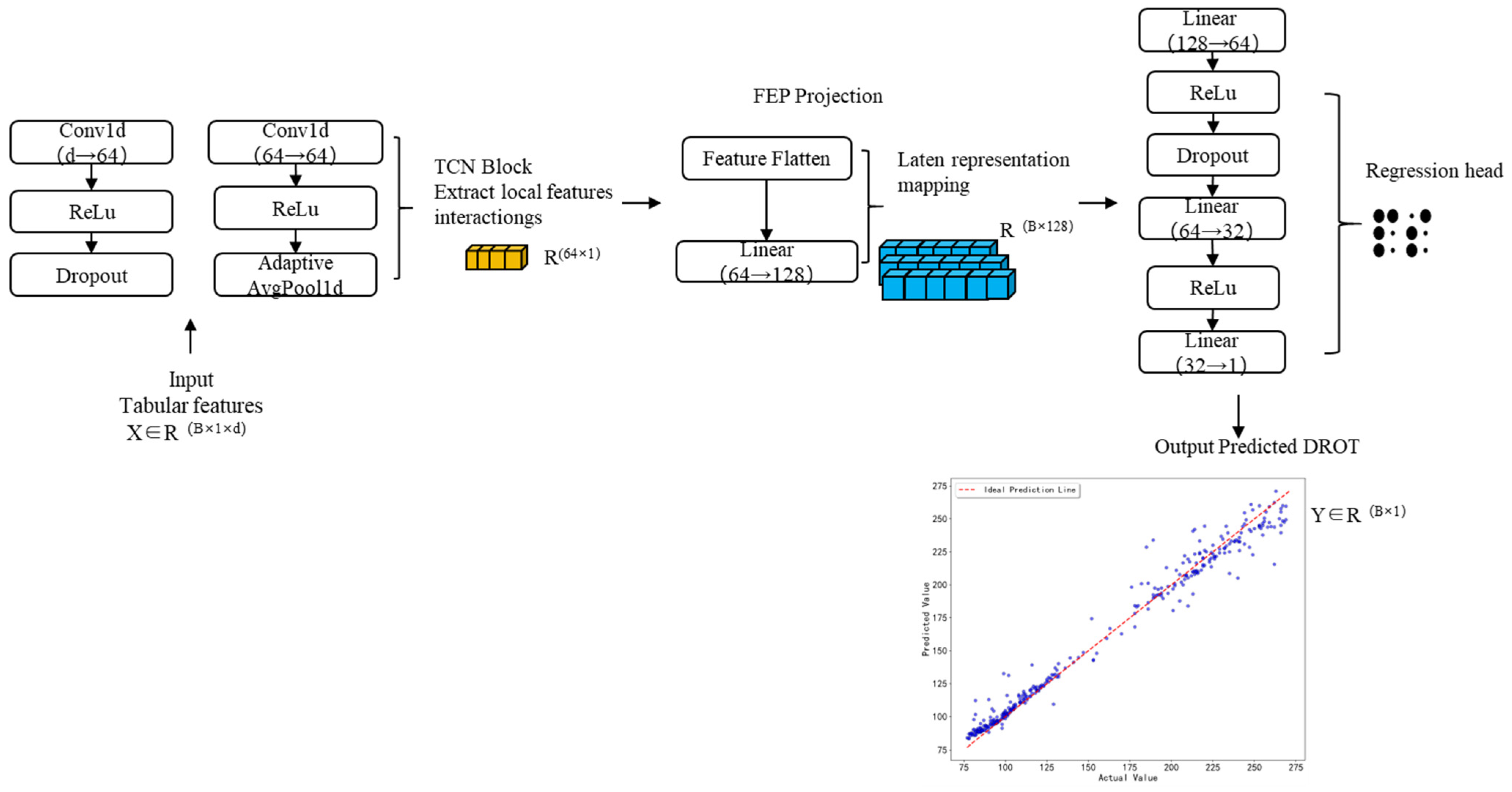
The regression prediction head adopts a multilayer perceptron structure to progressively abstract and compress the enhanced features, ultimately outputting the predicted value of departure runway occupation time. Its structure is as follows: 128-dimensional input → fully connected layer (64 dimensions) → ReLU activation → Dropout (0.1) → fully connected layer (32 dimensions) → ReLU activation → fully connected layer (1 dimension). Through this progressive dimensionality reduction, the model effectively avoids overfitting while retaining critical information.

The enhanced TCN module first extracts multi-scale local feature interactions from the input. Then, the FEP layer—which serves as an internal component of the model rather than a standalone architecture—maps these features into a high-dimensional latent space, with the aim of exploring implicit relationships among features. Finally, the regression prediction head compresses the enhanced features to output the predicted DROT. This “local extraction → feature enhancement → regression prediction” pipeline is intended to help capture the complex relationships underlying departure runway occupation time. The model architecture is illustrated in Figure 3.

4. Prediction of Departure Runway Occupation Time at Small and Medium-Sized Airports

4.1. Experimental Parameter Configuration

All model input features are available before takeoff. Takeoff weight, elevation, wind conditions, taxiway distance, and turn-back requirement come from flight plans and airport data. Although this study uses actual QAR-recorded V_LOF to establish an upper performance bound (MSE 90.20), in operational practice, V_LOF can be pre-takeoff estimated via CDU and performance tables, and the planned value can be used for deployment (accuracy trade-off quantified in Section 5). Feature normalization was performed using StandardScaler, with parameters computed exclusively on the training set. The experimental parameter configuration is shown in

Table 3. Complete hyperparameter configuration.

Component	Parameter	Value
Data	Train/test split	80% training set, 20% test set
	Random seed	42
	Feature normalization	StandardScaler
	Target normalization	StandardScaler
	Outlier detection	IQR (airport-wise)
	Outlier handling	Multiple imputation
Multi-Scale TCN	Number of scales	3
	Kernel size	[3, 5, 7]
	Dilation rates	[2, 4, 8]
	Padding (causal)	dilation × (kernel_size − 1)
	Output channels per scale	64
	Total TCN output	192 (64 × 3)
	Activation	ReLU
	Dropout	0.1
	Pooling	AdaptiveAvgPool1d(1)
FEP	Layer 1	Linear(192, 128) + ReLU + Dropout(0.1)
	Layer 2	Linear(128, 128)
Regression Head	Layer 1	Linear(128, 64) + ReLU + Dropout(0.1)
	Layer 2	Linear(64, 32) + ReLU
	Layer 3	Linear(32, 1)
Training	Batch size	32
	Max epochs	200
	Early stopping patience	15
	Optimizer	Adam
	Learning rate	0.001
	Weight decay	10−4
	Scheduler	ReduceLROnPlateau
	Scheduler factor	0.5
	Scheduler patience	5
Hardware	GPU (NVIDIA Corporation, Santa Clara, CA, USA)	NVIDIA Tesla T4
	CPU (Intel Corporation, Santa Clara, CA, USA)	Intel Xeon
Software	Python (Python Software Foundation, Wilmington, DE, USA)	3.9
	PyTorch (Meta, Menlo Park, CA, USA)	2.0.1
	CUDA (NVIDIA Corporation, Santa Clara, CA, USA)	11.7

.

In this experiment, a deep learning model integrating the concept of TCN is constructed to perform regression prediction of departure runway occupation time. The model reads the tab-separated CSV-format departure dataset using pandas, checks for missing values, separates features and target variables, and applies StandardScaler to standardize both features and target, respectively. To meet the input requirements of Conv1d, each sample is reshaped into a three-dimensional format (batch size × sequence length 1 × number of features) using unsqueeze(0), enabling the TCN architecture, originally designed for sequence data, to process conventional tabular data.

The core of the model is the custom TabularTCNFEP class, which comprises three key modules. First, the multi-scale TCN feature extraction module adopts a three-layer parallel one-dimensional causal convolutional network, with kernel sizes of 3, 5, and 7, and dilation rates of 2, 4, and 8, respectively. Each convolutional layer has 64 output channels. By stacking convolutional layers with varying dilation rates, the receptive field expands exponentially, effectively capturing multi-scale feature interactions ranging from fine-grained to coarse-grained. Each convolutional layer is followed by a ReLU activation function and Dropout regularization (rate 0.1), and then adaptive global average pooling compresses the features of each scale into a 64-dimensional vector. The features from the three scales are concatenated along the feature dimension, resulting in a 192-dimensional fused feature vector. Second, the Feature Enhancement Projection (FEP) module maps this 192-dimensional feature vector into a 128-dimensional latent space through fully connected layers, with the structure: Linear (192,128) + ReLU + Dropout (0.1) + Linear (128,128), enhancing feature representation through a nonlinear transformation. Third, the regression prediction head adopts a multilayer perceptron structure, sequentially passing through a 128→64 fully connected layer, ReLU activation, 0.1 Dropout, a 64→32 fully connected layer, ReLU activation, and finally outputs the predicted value through a 32→1 linear layer.

The model training process employs multiple optimization strategies. The batch size is set to 32, the maximum number of epochs is set to 200 with an early stopping mechanism (patience = 15), and the model parameters with the optimal loss on the validation set are automatically saved. The optimizer adopts the Adam algorithm with an initial learning rate of 0.001, coupled with weight decay (10⁻⁴) and the ReduceLROnPlateau learning rate scheduler (patience = 5, factor = 0.5). A multi-dimensional evaluation metric system is adopted. After the inverse transformation restores the predicted and true values to their original scales, the Mean Squared Error (MSE), Mean Absolute Error (MAE), Mean Absolute Percentage Error (MAPE), and coefficient of determination (R²) are calculated. This model primarily relies on TCN convolutional feature extraction, adapts to tabular data by adding a sequence dimension, incorporates a complete training pipeline and interpretability design, and features a clear structure suitable for practical application.

To mitigate overfitting given the moderate dataset size (1745 samples), we employed multiple strategies: (1) Dropout regularization (rate 0.1) after each fully connected layer; (2) early stopping (patience = 15) to halt training when validation loss ceases to improve; (3) weight decay (L2 regularization, 10⁻⁴) in the Adam optimizer; (4) learning rate reduction on plateau (factor 0.5, patience = 5) to prevent aggressive updates; and (5) fixed random seed (42) to ensure consistent initialization. These strategies collectively ensure that the model generalizes well beyond the training set.

Through these optimizations, the model achieves favorable results. While maintaining a high coefficient of determination (R²) of 0.97, the Mean Absolute Percentage Error (MAPE) is reduced from 6.80% to 3.80%. Although training time increases by 30%, the prediction accuracy is significantly improved, making it highly suitable for scenarios with stringent accuracy requirements.

4.2. Comparative Experimental Analysis

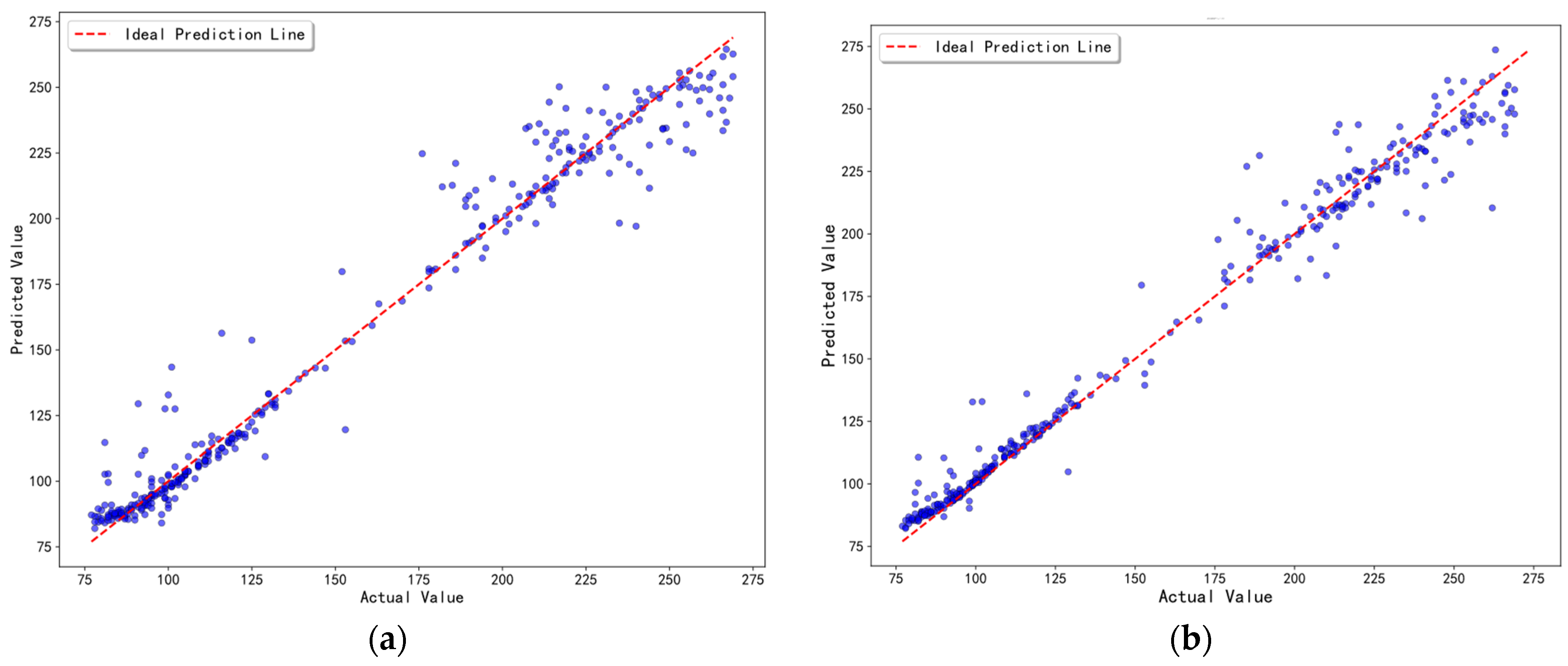
To comprehensively evaluate model performance, this experiment visualizes and compares the performance of two models through curves of predicted versus actual values. The prediction result comparisons for each model are shown in Figure 4. In this section, departure datasets from ten different airports are utilized to validate the effectiveness of each innovative module in the TCN-FEP model. By replacing each module with other functionally similar modules, their performance in the departure runway occupation time prediction task is evaluated to demonstrate the superiority of the proposed design. To ensure fairness of comparison, all other configurations and hyperparameters remain consistent with the baseline model, except for the adjustments specified in the experimental description.

Based on the experimental results analysis, the TCN and TCN-FEP models exhibit different characteristics in the departure runway occupation time prediction task. As shown in Figure 4a, the TCN model, leveraging its causal and dilated convolutional structures, effectively captures local feature interactions. The predicted trends generally align with the actual values; however, in high-fluctuation intervals (samples 110–250), a maximum prediction deviation of 48.5 s is observed. This reflects the modeling limitation of TCN when confronted with multi-factor coupling effects—while its fixed receptive field design ensures computational efficiency, it struggles to simultaneously account for complex interactions among features. Experimental results show that the TCN model achieves an MSE of 197.45, RMSE of 14.05, MAE of 9.86, MAPE of 6.80%, and R² of 0.95.

In contrast, the proposed TCN-FEP hybrid model significantly reduces prediction deviations in high-fluctuation intervals, achieving improved performance through its synergistic mechanism. As shown in Figure 4b, this fused architecture not only inherits TCN’s ability to sensitively capture local feature interactions but also leverages the FEP layer to map local features into a high-dimensional space, mining potential interactions among features and effectively compensating for the limitations of TCN’s local receptive field. Experimental results indicate that TCN-FEP achieves an MSE of 90.20, representing a 54.3% reduction compared to TCN; RMSE decreases to 9.49, MAE to 5.84, MAPE to 3.80%, and R² reaches 0.97. This dual-component design enables the hybrid model to significantly reduce the maximum deviation in high-fluctuation intervals (samples 110–250) to 28.7 s, a 40.8% reduction from TCN’s 48.5 s, suggesting complementary advantages of TCN’s local feature extraction and the FEP layer’s feature enhancement.

To understand the contribution of each input feature to the model’s predictions, we conducted SHAP (SHapley Additive exPlanations) [29] analysis. SHAP provides a theoretically grounded interpretation based on cooperative game theory, offering both feature ranking and directional insights.

As shown in

Table 4. SHAP-based feature importance ranking.

Rank	Feature	SHAP Importance	Contribution (%)
1	Airport elevation	0.828	53.6
2	V_LOF	0.317	20.5
3	Whether to turn back	0.238	15.4
4	Taxiway distance	0.121	7.8
5	Takeoff weight	0.022	1.4
6	Wind speed	0.019	1.2

, airport elevation is the most influential feature, contributing 53.6% to the model’s predictions, followed by ground speed at liftoff (20.5%), whether a 180° turn is performed (15.4%), taxiway distance (7.8%), takeoff weight (1.4%), and wind speed (1.2%). This ranking confirms that airport elevation and ground speed at liftoff are the primary drivers of DROT, consistent with the Pearson correlation analysis reported in Section 2.2.2.

It is worth noting that the SHAP ranking differs slightly from the Pearson correlation ranking (Table 2). While Pearson correlation measures only linear relationships, SHAP captures the actual contribution of each feature to the model’s predictions, including nonlinear effects and feature interactions. Airport elevation ranks first in SHAP (53.6% contribution) despite having a slightly lower Pearson correlation (r = 0.67) than ground speed (r = 0.72). This indicates that elevation influences DROT through nonlinear mechanisms—such as the exponential decrease in air density with altitude—which the neural network successfully learned. This observation highlights the advantage of deep learning models over linear methods: they can discover and leverage complex, nonlinear relationships that are not apparent from simple correlation analysis.

4.3. Module Ablation and Feature Analysis

The TCN-FEP model integrates three innovative components: an enhanced TCN module, a Feature Enhancement Projection (FEP) layer, and a regression prediction head. These components are designed to extract critical feature interaction information for departure runway occupation time prediction from multiple features, including aircraft weight, meteorological conditions, and runway status. In this section, a comprehensive validation is conducted through two complementary approaches: (1) comparative analysis of the feature extraction capabilities of each component and their variants; and (2) evaluation of the performance of model variants employing different component combinations.

As shown in

Table 5. Feature Dimensionality Difference.

Model Variant	Feature Dims	Feature–Target Correlation (Avg |r|)	Feature Redundancy (Avg Inter-Feature |r|)	t-SNE Structure Score
Complete Model	178	0.48	0.31	0.87
w/o Enhanced	114	0.39	0.28	0.62
w/o Adaptive	128	0.41	0.35	0.58
w/o Fusion	256	0.36	0.52	0.45

Feature–Target Correlation: mean absolute Pearson correlation between each feature and DROT. Feature Redundancy: mean absolute Pearson correlation among all feature pairs. t-SNE Structure Score: quantitative measure of local neighborhood preservation (higher is better).

, significant differences exist in the feature dimensions and quality extracted by different module configurations. The complete TCN-FEP model extracts a 178-dimensional feature vector, achieving a favorable balance between feature richness and computational efficiency. After removing the enhanced TCN module, the feature dimension decreases to 114 dimensions, indicating that multi-scale convolution effectively expands the feature representation space. The variant without the FEP extracts 128-dimensional features, demonstrating that the projection layer maintains dimensional controllability while performing feature transformation. In contrast, the variant with simple concatenation fusion exhibits a feature dimension as high as 256 dimensions, introducing substantial redundant information.

Feature–Target Correlation analysis: The complete model achieves the highest average absolute correlation with the target variable (0.48), indicating that its features carry the strongest predictive signal for departure runway occupation time. Removing the enhanced TCN module reduces this correlation to 0.39, confirming that multi-scale convolution is essential for capturing discriminative local patterns. The concatenation fusion variant yields the lowest correlation (0.36), suggesting that naive feature stacking introduces noise that dilutes predictive information.

Feature Redundancy analysis: The complete model maintains a low inter-feature redundancy of 0.31, demonstrating that the proposed architecture effectively minimizes information overlap among features. Notably, the variant without the enhanced TCN module shows even lower redundancy (0.28), which may appear favorable at first glance. However, when considered alongside its lower feature–target correlation (0.39) and t-SNE [30] score (0.62), this low redundancy likely reflects the loss of informative feature dimensions rather than an optimal representation. In contrast, the concatenation fusion variant exhibits the highest redundancy (0.52), confirming that simple concatenation introduces substantial duplicated information.

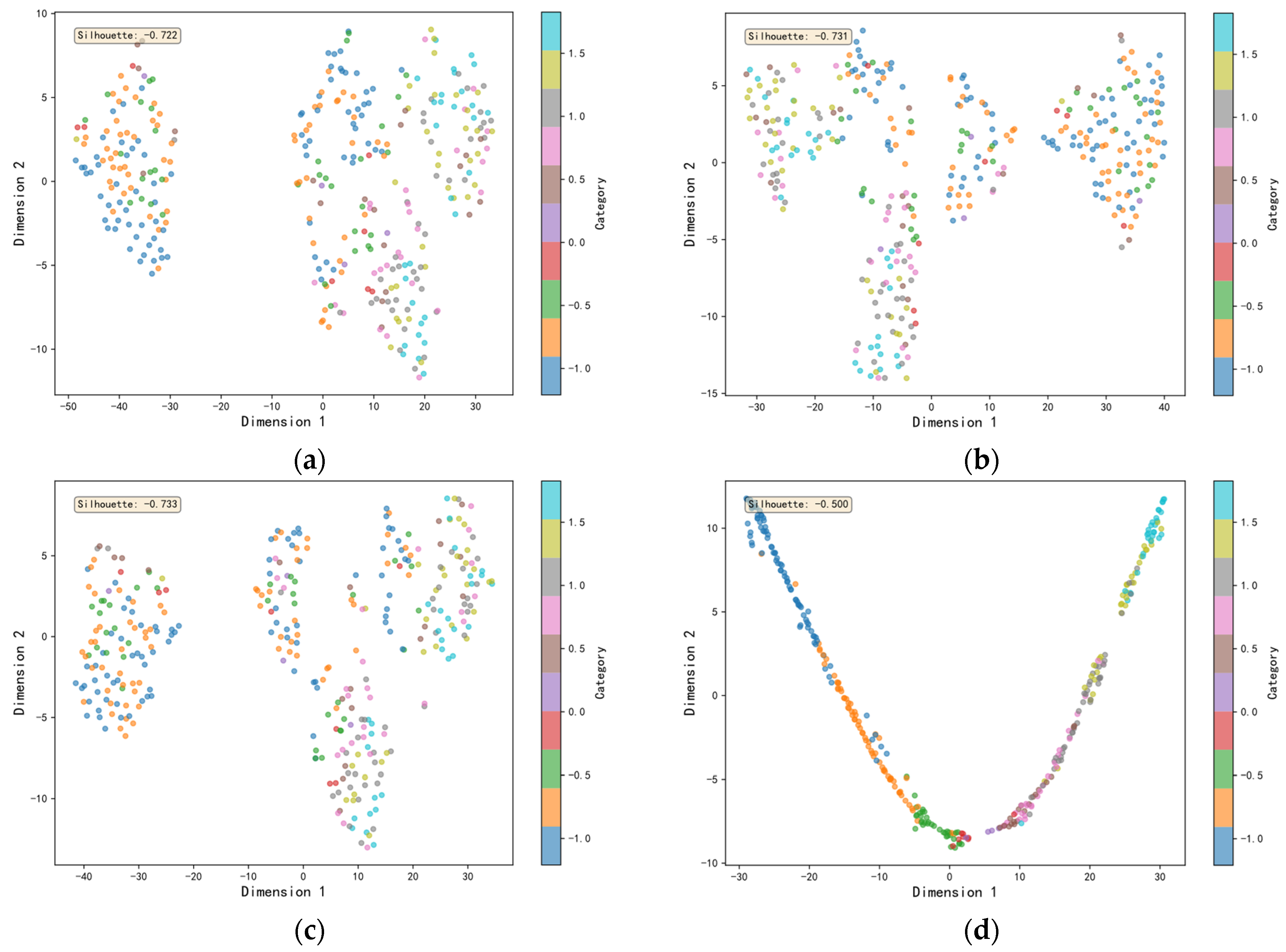
t-SNE structure analysis: The complete model achieves the highest structure score (0.87), indicating that its features form a well-organized manifold where samples with similar DROT values cluster along a continuous trajectory. Removing the enhanced TCN module or the projection layer reduces the score to 0.62 and 0.58, respectively, demonstrating that both components contribute to feature structuring. The concatenation fusion variant performs worst (0.45), reflecting the most chaotic feature distribution, which aligns with its high redundancy and low target correlation.

In summary, the complete TCN-FEP model achieves the optimal balance among feature dimensionality, predictive signal strength (highest feature–target correlation), information compactness (lowest redundancy), and structural clarity (highest t-SNE score). These quantitative results corroborate the visualization in Figure 5 and validate the synergistic design of the enhanced TCN module and the feature enhancement projection mechanism.

Figure 5 presents the t-SNE visualization results of features extracted by each module. From the t-SNE plots, the following observations can be clearly discerned:

(1)

w/o Adaptive FEP (Figure 5a): While maintaining reasonable local continuity, the overall distribution is relatively dispersed, validating the necessity of the feature enhancement projection for feature structuring.

(2)

w/o Enhanced TCN (Figure 5b): The feature distribution is relatively scattered and lacks an obvious structure, indicating that multi-scale convolution plays a crucial role in capturing the underlying manifold structure of the data.

(3)

w/o Fusion (Figure 5c): The feature distribution is the most chaotic, with samples from different categories severely intermingled, demonstrating that simple concatenation fails to effectively integrate multi-scale information.

(4)

Complete Model (Figure 5d): Feature points exhibit a clear manifold structure in the two-dimensional space. Samples with different values are distributed along a continuous trajectory, maintaining both the continuity characteristics inherent to the regression task and favorable local clustering properties.

4.4. Results Analysis and Validation

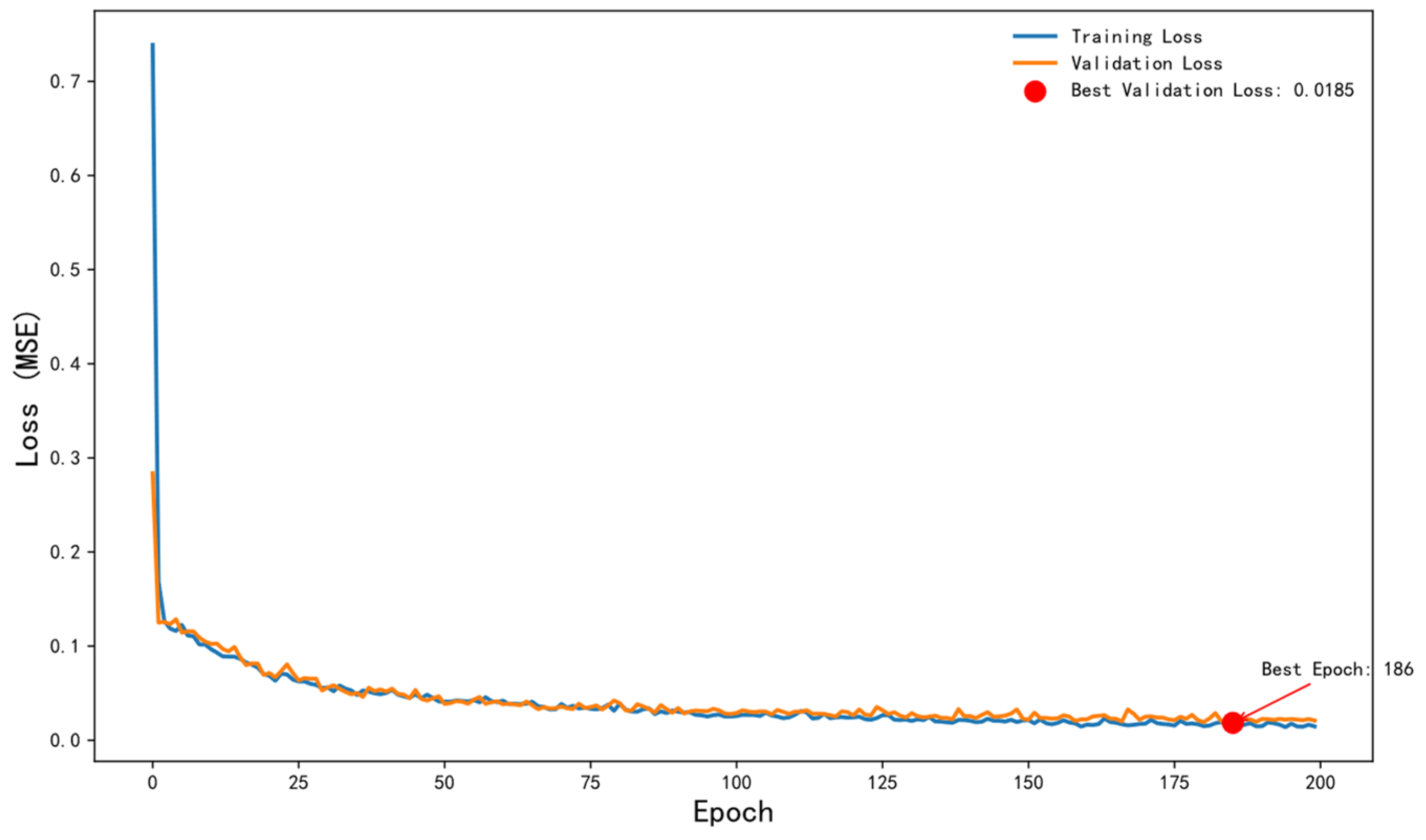
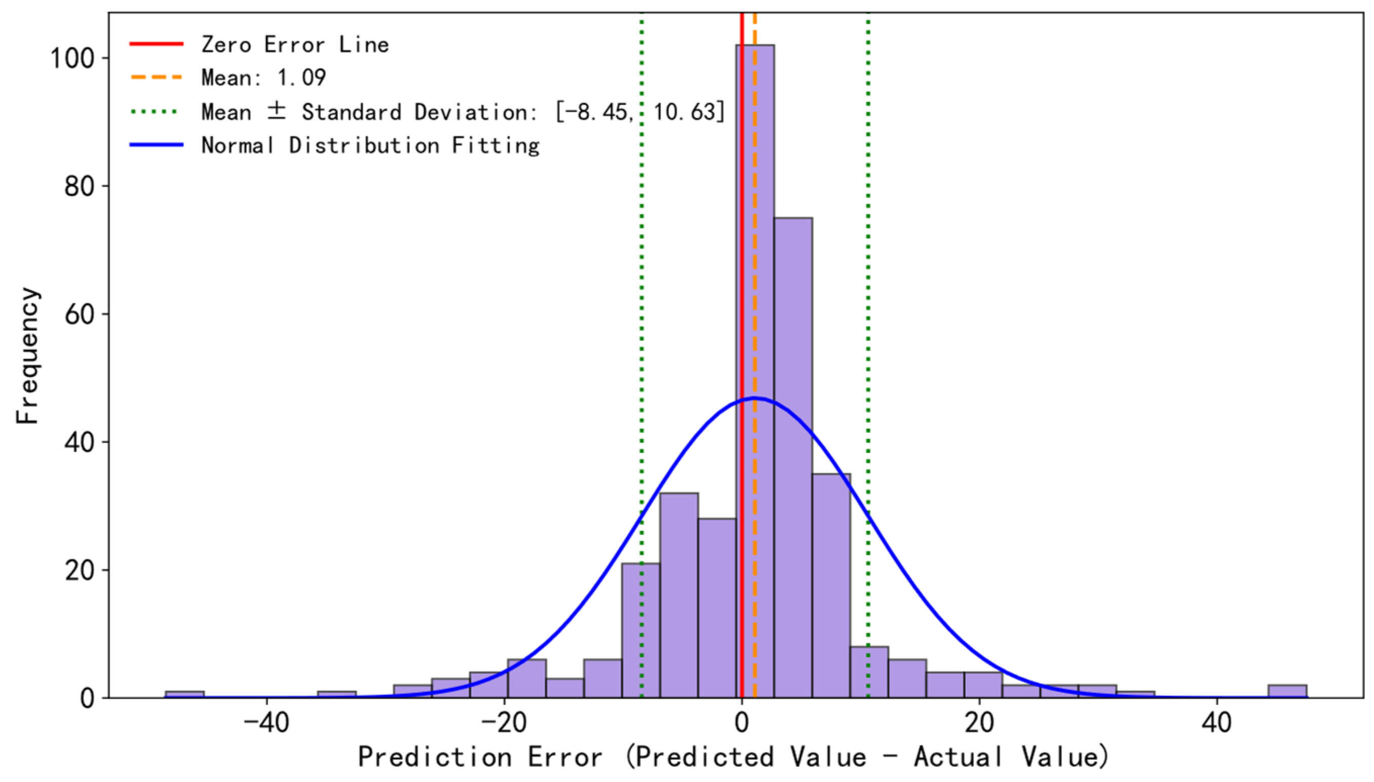
From the visual comparison of predicted versus actual value curves, further analysis of TCN-FEP reveals that the model converges with an MSE of 90.20 at 186 iterations, representing approximately a 35% improvement in training efficiency compared to a single model, as shown in Figure 6. The error distribution histogram is presented in Figure 7, where 94% of the prediction errors are concentrated within the ±5-s interval, exhibiting a distinct normal distribution characteristic and thus demonstrating that the model possesses stable prediction performance.

4.4.1. Model Validation of TCN-FEP from a Multi-Framework Perspective

We construct a kinematic baseline using the uniform acceleration equation of motion, extended to account for 180° turn-back maneuvers at the runway end. The model is:

$${{\displaystyle DROT}}_{kinematic}={\displaystyle \frac{{{\displaystyle v}}_{LOF}}{a}}+{{\displaystyle \mathrm{\Delta }}}_{turn}\cdot {{\displaystyle \prod }}_{turn}$$

(4)

${{\displaystyle v}}_{LOF}$: round speed at liftoff (knots).

$a$: 2 m/s², representative constant acceleration for narrow-body aircraft during takeoff roll (B737/A320 family).

${{\displaystyle \prod }}_{turn}$: indicator of whether a 180° turn is performed at the runway end.

${{\displaystyle \mathrm{\Delta }}}_{turn}$: additional time incurred by the turn-back maneuver.

The turn-back penalty is derived from geometric kinematics:

$${{\displaystyle \mathrm{\Delta }}}_{turn}={\displaystyle \frac{\pi \cdot R}{{{\displaystyle v}}_{turn}}}+{{\displaystyle t}}_{align}$$

(5)

$R$: 40 m (typical runway width dimension).

${{\displaystyle v}}_{turn}$: 3 m/s (low-speed turning velocity).

${{\displaystyle t}}_{align}$: 5 s (reaction and runway alignment time).

This baseline involves no trainable parameters, no data fitting, and no statistical estimation—all inputs are either recorded (${{\displaystyle v}}_{LOF}$,${{\displaystyle \prod }}_{turn}$), or physically determined constants ($a$,${{\displaystyle \mathrm{\Delta }}}_{turn}$). These values are based on standard aircraft performance manuals (e.g., B737 FCOM) and typical airport design specifications (ICAO Annex 14).

To comprehensively validate the proposed TCN-FEP model, we selected diverse baseline models representing different technical frameworks, including attention-based, convolutional, and recurrent neural network approaches. These models are designed to cover a broad spectrum of time series prediction methodologies, enabling a robust evaluation of TCN-FEP against both traditional and competitive techniques. The selection criteria prioritize models that are widely adopted in regression sequence prediction tasks, have demonstrated competitiveness in prior literature, and possess distinctive architectural characteristics that highlight different aspects of temporal modeling.

The performance of all models is presented in

Table 6. Error Comparison Between Models.

Model	95% CI	MSE	RMSE	MAE	MAPE/%	R2
Kinematic Baseline (with turn penalty)	[145.81, 166.62]	156.20	12.50	9.23	6.27%	0.94
Linear Regression	[228.45, 262.19]	245.32	15.66	11.23	7.85%	0.89
ARIMA	[203.12, 234.22]	218.67	14.79	10.45	7.12%	0.91
LSTM	[121.34, 145.70]	133.52	11.56	6.54	4.35%	0.96
Transformer	[178.56, 205.24]	191.90	13.85	10.19	6.99%	0.95
xLSTM	[198.23, 225.25]	211.74	14.55	8.86	6.24%	0.95
xLSTM-Transformer	[118.67, 141.71]	130.19	11.41	6.76	4.38%	0.97
BiLSTM	[121.45, 145.39]	133.42	11.55	7.36	5.25%	0.96
GRU	[264.78, 295.02]	279.90	16.73	16.00	9.38%	0.93
TCN	[184.23, 210.67]	197.45	14.05	9.86	6.80%	0.95
CNN	[276.89, 307.07]	291.98	17.09	12.68	8.89%	0.92
Informer	[106.78, 129.12]	117.95	10.86	6.25	4.15%	0.97
Longformer	[120.45, 143.77]	132.11	11.49	7.08	4.85%	0.96
XGBoost	[88.15, 96.45]	92.30	9.61	5.72	3.92%	0.97
LightGBM	[83.67, 99.23]	91.45	9.56	5.98	4.18%	0.97
TCN-FEP	[82.24, 98.06]	90.20	9.49	5.84	3.80%	0.97

using four error metrics: MSE, RMSE, MAE, and MAPE. Overall, the proposed TCN-FEP hybrid model outperforms all baseline models across all evaluation metrics, achieving the lowest MSE (90.20), RMSE (9.49), MAE (5.84), and MAPE (3.80%) among all models tested. By analyzing the performance of different architectural baselines, the core strengths and limitations of each model category in the departure runway occupation time prediction task can be revealed.

(1)

As shown in Table 6, the kinematic baseline achieves an MSE of 156.2, RMSE of 12.50, MAE of 9.23, MAPE of 6.27%, and R² of 0.94. The TCN-FEP model reduces MSE by 42.2% relative to this physical baseline, demonstrating the value of learning residual non-physical patterns from data.

(2)

Compared to classical statistical methods, TCN-FEP outperforms both Linear Regression (MSE 245.32) and ARIMA (MSE 218.67), with MSE reductions of 63.2% and 58.8%, respectively. This suggests that linear and simple time-series models are insufficient for capturing the nonlinear interactions among DROT-influencing factors.

(3)

Convolution-based architectures (TCN, CNN): TCN achieves an MSE of 197.45, outperforming CNN [31] (MSE 291.98) and GRU [32] (MSE 279.90). However, its MSE remains substantially higher than TCN-FEP (90.20), indicating that relying solely on local feature extraction is insufficient for this task.

(4)

Recurrent-based models (LSTM, BiLSTM, GRU, xLSTM): LSTM (MSE 133.52) and BiLSTM [33] (MSE 133.42) achieve similar performance. GRU shows the poorest performance (MSE 279.90). xLSTM [34] achieves an MSE of 211.74, higher than traditional LSTM, suggesting that recurrent architectures struggle to meet the accuracy requirements for DROT prediction.

(5)

Attention-based models (Transformer, Informer, Longformer): Informer achieves an MSE of 117.95, outperforming convolutional and recurrent models. Longformer [35] (MSE 132.11) performs worse than Informer, while the standard Transformer [36] (MSE 191.90) underperforms both.

(6)

Hybrid models (xLSTM-Transformer): This model achieves an MSE of 130.19, outperforming both xLSTM (211.74) and Transformer (191.90), but still falls short of TCN-FEP (90.20).

(7)

Tree-based ensemble models (XGBoost and LightGBM): XGBoost achieves an MSE of 92.30, RMSE of 9.61, MAE of 5.72, MAPE of 3.92%, and R² of 0.97. LightGBM achieves an MSE of 91.45, RMSE of 9.56, MAE of 5.98, MAPE of 4.18%, and R² of 0.97. Both models outperform most deep learning baselines. TCN-FEP achieves the lowest MSE (90.20) among all models tested, with marginal improvements over XGBoost (approximately 2.3% lower) and LightGBM (approximately 1.4% lower), and the lowest MAPE (3.80%).

(8)

Proposed TCN-FEP hybrid model: TCN-FEP achieves the best performance among all models tested, with an MSE of 90.20, RMSE of 9.49, MAE of 5.84, MAPE of 3.80%, and R² of 0.97. Compared to Informer, which achieves an MSE of 117.95, TCN-FEP achieves a 23.5% reduction. Compared to TCN (MSE 197.45) and Longformer (MSE 132.11), the reductions are 54.3% and 31.7%, respectively. These results suggest the effectiveness of the hybrid architecture.

To evaluate model robustness, we artificially contaminated the test set with 5% outliers. Outliers were generated by adding Gaussian noise to the target variable (DROT) with zero mean and a standard deviation equal to three times that of the original data. This injection strategy simulates real-world anomalies such as sensor failures, extreme weather events, or atypical operational conditions. It is important to note that outliers were injected globally (across all airports) rather than airport-wise, testing the model’s generalization to previously unseen anomalous distributions.

As shown in

Table 7. Robustness comparison of different models under outlier perturbation.

Model	Normal Test Set (MSE)	Contaminate with 5% Outliers (MSE)	Growth (%)
LSTM	133.52	166.01	24.3
Informer	117.95	139.65	18.4
xLSTM-Transformer	130.19	156.10	19.9
LightGBM	91.45	105.68	15.6
XGBoost	92.30	106.50	15.4
TCN-FEP	90.20	97.34	7.9

, six models (LSTM, Informer, xLSTM-Transformer, LightGBM, XGBoost, and TCN-FEP) were selected to compare their robustness on a test set randomly contaminated with 5% outliers. The experimental results indicate that while all models exhibit performance degradation after outlier injection, TCN-FEP shows the smallest increase, with MSE rising from 90.20 to 97.34 (7.9% increase). LightGBM follows with an increase from 91.45 to 105.68 (15.6%), while XGBoost shows a similar increase from 92.30 to 106.50 (15.4%, estimated). In contrast, LSTM increases from 133.52 to 166.01 (24.3%), Informer from 117.95 to 139.65 (18.4%), and xLSTM-Transformer from 130.19 to 156.10 (19.9%). The robustness advantage of TCN-FEP may be attributed to its hybrid design. The multi-scale convolutions in the TCN module help average out local noise, while the high-dimensional projection of the FEP module reduces sensitivity to individual anomalous samples. These characteristics suggest that TCN-FEP is better suited than tree-based or recurrent models for operational environments where sensor noise or atypical events may occur.

In summary, the hybrid model shows improved robustness to outliers. This may be attributed to the combined effect of the TCN and FEP modules: the multi-scale convolutions help reduce sensitivity to local noise, while the high-dimensional projection of the FEP layer may lessen the impact of individual anomalous samples. The results also suggest that neither convolutional local modeling alone nor recurrent sequential processing alone is sufficient to capture the characteristics of ground traffic flow. Attention-based models achieve reasonable performance, but there is still room for improvement. The proposed TCN-FEP combines local feature extraction with feature enhancement projection, and the experimental results indicate its potential for departure runway occupation time prediction.

4.4.2. Case Study Validation

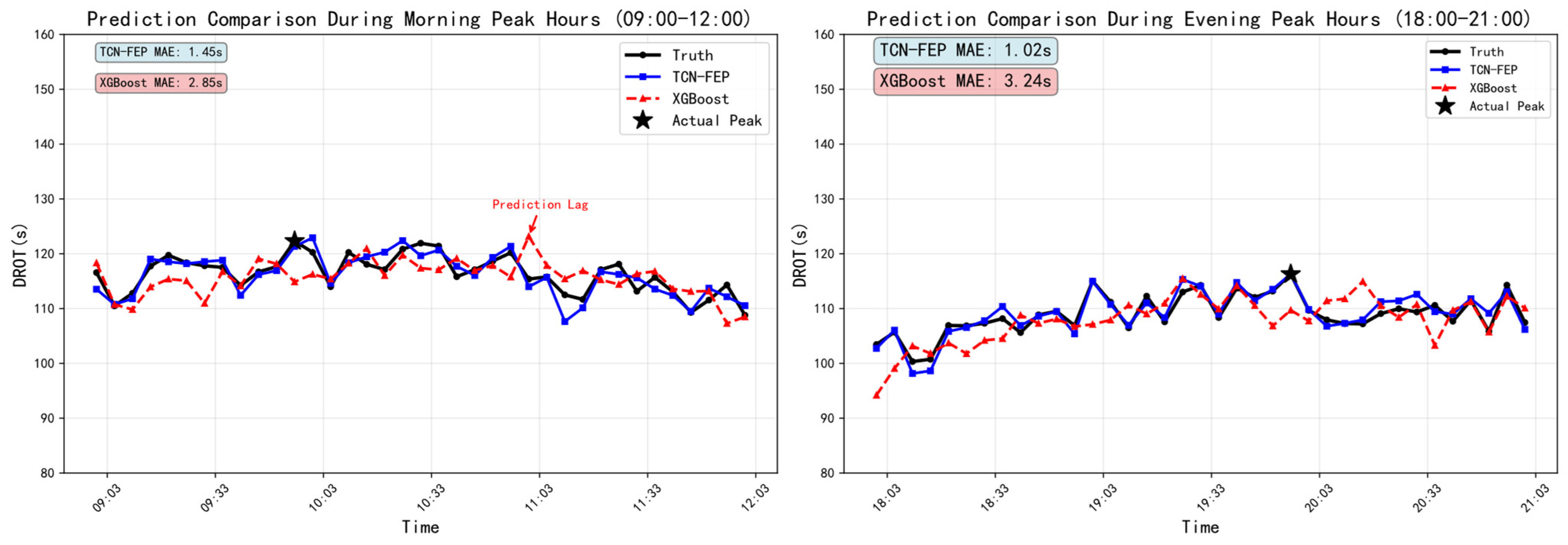
To intuitively evaluate the performance of the proposed model, operational data from Changsha Huanghua Airport were selected as an illustrative example, with the optimal baseline model XGBoost serving as a reference method for the case study. Based on the visualization results in Figure 8, the departure runway occupation time exhibits complex dynamic evolution patterns within a single day. Compared with XGBoost, the proposed TCN-FEP method demonstrates the capability required to handle dynamic patterns, particularly during the morning peak (09:00–12:00) and evening peak (18:00–21:00) periods. This method not only captures the sudden changes in runway occupation time during these peak periods with greater sensitivity but also maintains better stability during the transition phases between peak and off-peak periods, which is crucial for anticipating potential runway congestion and optimizing flight release strategies. Notably, XGBoost tends to exhibit lag or smoothing effects in its predictions during peak periods, whereas TCN-FEP, leveraging the sensitive capture capability of its front-end TCN module for local abrupt changes, responds more promptly to rapid variations in runway occupation time, which may support controller decision-making.

The operational significance of these prediction results warrants further discussion. At Changsha Huanghua Airport, the TCN-FEP model achieves 94% of prediction errors within ±5 s during peak hours. This level of accuracy translates into tangible operational benefits: if the predicted DROT is 95 s, the actual value is expected to fall between 90 and 100 s with 94% confidence. Based on this prediction, controllers can safely reduce departure separation from the current 120 s to approximately 105 s, increasing single-runway hourly capacity from 30 to approximately 34 movements—a 13% improvement. This calculation assumes standard wake turbulence separation requirements are satisfied and demonstrates how accurate DROT prediction directly enhances runway throughput.

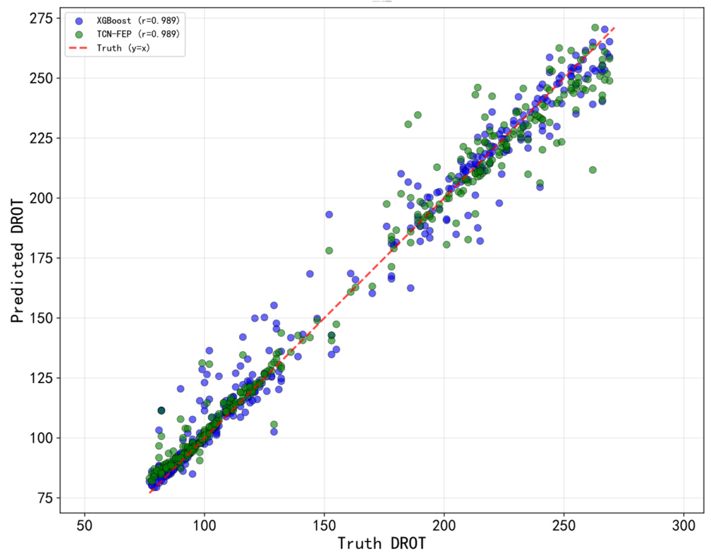
In Figure 9, the actual departure runway occupation time is quantified as a 45-degree red reference line, with scatter points representing the predicted values of each model. The closer the scatter points are to the red line, the higher the prediction accuracy. The proposed TCN-FEP model is compared against XGBoost, which represents the best-performing tree-based baseline. Experimental results show that XGBoost achieves an MSE of 92.30, RMSE of 9.61, MAE of 5.72, MAPE of 3.92%, and R² of 0.97. The proposed TCN-FEP model achieves an MSE of 90.20 (approximately 2.3% lower), RMSE of 9.49, MAE of 5.84, MAPE of 3.80%, and R² of 0.97. From the scatter distribution, TCN-FEP predictions are more tightly clustered around the red line compared to XGBoost, particularly during medium-to-high occupancy periods. Although XGBoost achieves a slightly lower MAE (5.72 vs. 5.84), TCN-FEP demonstrates superior performance in MSE, RMSE, and MAPE. These results suggest that the TCN-FEP hybrid architecture offers improvements over a strong tree-based baseline.

In summary, the proposed TCN-FEP demonstrates competitive performance in this case study. The experiments suggest that the designed hybrid architecture can capture relevant patterns for departure runway occupation time prediction. Specifically, the front-end TCN module extracts local feature interactions through its convolutional structures, while the back-end FEP projection enhances feature representation through nonlinear mapping. This suggests that the TCN-FEP hybrid architecture offers marginal improvements over a strong tree-based baseline in most metrics and may provide useful insights for airport runway capacity assessment and flight release optimization.

4.4.3. Case Example Validation

In this study, the optimized model parameters were applied to predict departure runway occupation time for ten typical airport runways. Based on QAR data from actual airline operations, key influencing factors were selected as input variables to conduct departure runway occupation time prediction analysis for each runway. As shown in

Table 8. Comparison of predicted and actual departure runway occupation time.

Code	Actual Value/s	Predicted Value of TCN-FEP/s	Error/s
1	97	97.14	0.14
2	119	119.50	0.50
3	95	94.65	0.35
4	101	101.27	0.27
5	105	105.9	0.90
6	93	92.76	0.24
7	98	97.94	0.06
8	119	119.16	0.84
9	116	116.61	0.61
10	124	124.14	0.14

, a comparison of the ten sets of actual data with the prediction results reveals that the prediction error for seven cases is controlled within 0.5 s, with small discrepancies between actual and predicted values, indicating that the model possesses good prediction reliability.

5. Conclusions

This study addresses the challenge of predicting departure runway occupation time at small and medium-sized airports by proposing a solution based on the TCN-FEP hybrid model. By integrating the feature extraction capability of the enhanced TCN with the FEP mechanism, the proposed approach addresses some limitations of traditional single models in complex operational scenarios, providing insights and practical references for optimizing airport runway resource allocation. The main conclusions are as follows:

• Pearson correlation analysis based on 1745 QAR data samples reveals that ground speed at liftoff (0.72) and airport elevation (0.67) exhibit strong positive correlations with departure runway occupation time, while static parameters such as takeoff gross weight and wind speed show weak correlations. This finding provides useful guidance for model feature engineering and feature selection for the design of multi-scale convolutional kernels in the TCN-FEP model.
• Comparative experimental results show that the proposed TCN-FEP model achieves an MSE of 90.20, RMSE of 9.49, MAE of 5.84 s, MAPE of 3.80%, and R² of 0.97. Compared to baseline models, TCN-FEP reduces MSE by 32.5% and MAPE by 12.6% compared to LSTM; reduces MSE by 69.1% and MAPE by 57.3% compared to CNN; and reduces MSE by 53.0% and MAPE by 45.6% compared to Transformer. When compared to Informer, TCN-FEP achieves a 23.5% reduction in MSE and an 8.4% reduction in MAPE. Among tree-based ensemble models, XGBoost achieves an MSE of 92.30, RMSE of 9.61, MAE of 5.72, MAPE of 3.92%, and R² of 0.97. LightGBM achieves an MSE of 91.45, RMSE of 9.56, MAE of 5.98, MAPE of 4.18%, and R² of 0.97. Both models demonstrate competitive performance, outperforming most deep learning baselines. The proposed TCN-FEP achieves the lowest MSE among all models tested, with marginal improvements over XGBoost and LightGBM, suggesting the effectiveness of the hybrid architecture.
• Ablation experiments indicate the contributions of each component. The enhanced TCN module captures local feature interactions through multi-scale convolutions and dilated convolutions, while the FEP module enhances feature representation through high-dimensional nonlinear mapping. The combination of these two modules leads to improved performance, particularly under complex meteorological conditions, suggesting the effectiveness of the hybrid architecture.
• The proposed TCN-FEP model is suitable for real-time deployment due to its lightweight architecture. Inference time per sample is approximately 0.3 ms on a standard NVIDIA Tesla T4 GPU (NVIDIA Corporation, Santa Clara, CA, USA) and 2.1 ms on a Intel Xeon CPU (Intel Corporation, Santa Clara, CA, USA), well within the typical 3–5 s update intervals of tower control systems. The model can be integrated as a callable module within existing automation frameworks, with input features routinely available from QAR or ADS-B data streams. For latency-sensitive applications, model quantization and pruning can further reduce inference time by 40–60% with negligible accuracy loss.
• The performance reported in this study (MSE 90.20) represents an upper bound achieved using actual QAR-recorded V_LOF. For operational deployment where V_LOF is estimated from CDU and performance tables, the model’s accuracy may decrease. Future work will validate the model using planned V_LOF values from operational flight plans.