Abstract
High-pressure compressor (HPC) blades of aero engines inevitably exhibit various uncertain geometric deviations, which deteriorate engine performance and increase maintenance costs. Although the condition-based maintenance (CBM) strategy is increasingly adopted to reduce costs by tailoring repair actions based on condition monitoring data, maintenance practices often still rely on original equipment manufacturer (OEM) recommendations. To further refine the CBM strategy, this paper proposes an uncertainty quantification method based on the engine performance digital twin (PDT) model to quantify the impact of HPC blade geometric deviations on overall engine performance. The PDT model is developed by coupling computational fluid dynamics simulations with a zero-dimensional performance model using real operating data and is validated for high predictive accuracy. Surrogate models based on support vector regression are employed to efficiently quantify the impact of combined geometric deviations. The results show that combined deviations cause reductions in mass flow, pressure ratio, and efficiency while increasing exhaust gas temperature and specific fuel consumption. The proposed methodology is applied to a CBM scenario to demonstrate its effectiveness. In the real maintenance process, this method enables the prediction of performance after repair, facilitating optimized maintenance strategies.
1. Introduction
As a critical component of an aero engine, the high-pressure compressor (HPC) supplies high-pressure air for fuel combustion, making its aerodynamic performance significantly impact the overall engine performance. Due to inevitable manufacturing errors, in-service erosion, fouling, and creep, various uncertain geometric deviations in HPC blades arise during both the manufacturing [1] and operating [2] phases. These deviations, characterized by uncertainty, contribute to performance deterioration and dispersion [3]. Once engine performance exceeds a specified limit, its deteriorated blades must be maintained according to the applied maintenance strategies. The traditional time-based maintenance strategy typically performs standard repairs on components at predetermined intervals, regardless of their real condition. This conservative strategy potentially results in unnecessary component repairs and replacements, leading to elevated maintenance costs. Excluding personnel and fuel expenses, maintenance, repair, and overhaul (MRO) costs account for approximately 10% of the total aircraft operating costs, with nearly 40% of these MRO expenses attributed to engine restoration [4].
To reduce costs, most state-of-the-art aero engines employ condition-based maintenance (CBM), which utilizes information acquired through condition monitoring to recommend repair actions [5]. However, in reality, many engines still have fixed intervals at which maintenance is performed based on original equipment manufacturer (OEM) recommendations corresponding to the measured geometric deviations of components. Due to differences in the real engine operating environment and the potential hidden agendas of OEMs to maximize spare parts replacement through a conservative maintenance strategy, such OEM-recommended repair procedures are not usually applicable when attempting to minimize costs [6]. To further refine CBM, it is essential to assess the impact of uncertain geometric deviations of deteriorated HPC blades on engine performance, thereby optimizing maintenance decisions for engine restoration.
Quantifying the forward propagation of uncertainty from blade geometric deviations to engine performance falls within the scope of uncertainty quantification theory [7]. Common methods for uncertainty quantification of various components in aero engines include sampling-based, sensitivity-based, and surrogate model-based methods [8]. Among sampling-based methods, Monte Carlo simulation (MCS) and its improved variants [9] are most commonly used. These methods generate random inputs by drawing samples from probability distributions and repeatedly performing deterministic computations to approximate the distributions of responses. Garzon et al. [10] employed the MCS method to quantify the uncertainty of the impact of blade geometric variations on compressor performance by constructing a probabilistic model of variations. The results indicate that compressor efficiency may decrease by approximately 1% due to representative manufacturing uncertainties in the blades. Lange et al. [11] conducted computational fluid dynamics (CFD) simulations on a multi-stage HPC model with 150 blades and employed the MCS method to identify HPC performance dispersion. However, processing a large number of samples in these studies incurs significant computational and time costs. Sensitivity-based methods leverage the Taylor series expansion to describe uncertainty propagation using derivatives of the objective function. These methods apply to high-dimensional uncertain variables and significantly reduce computational costs. Giebmanns et al. [12] employed the adjoint method within sensitivity-based approaches to determine the sensitivity of compressor performance to seven geometric uncertainty factors. Xu et al. [13] proposed an adjoint-based nonlinear approach, denoted as MC-adj-nonlinear, to enable a more accurate and efficient evaluation of the impact of blade section geometric deviations on compressor performance.
Compared to the first two methods, surrogate model-based methods achieve a balance between computational cost and accuracy by constructing a surrogate model that approximates the original mapping. Commonly used surrogate models include the Kriging model and its variants [14], non-intrusive polynomial chaos expansion (NIPC) [15], neural networks [16], response surface model [17], and the support vector regression (SVR) model [18]. He et al. [19] employed a neural network-based surrogate model to predict the performance of a centrifugal compressor under geometric uncertainty. Ma et al. [20] utilized both the Kriging model and NIPC to quantify the uncertainty induced by manufacturing errors in compressor blades. They conducted a robust blade optimization design considering manufacturing errors and proposed an optimization scheme that reduced the sensitivity of aerodynamic performance to manufacturing errors.
The aforementioned studies are limited to quantifying the uncertainty propagation from blade geometric deviations to HPC aerodynamic performance. Quantifying the impact on overall engine performance is crucial to the real CBM. Kraft et al. [21] developed high-accuracy engine performance models to evaluate the impact of blade geometric variations on overall performance, thereby assisting in maintenance decision optimization. Reitz et al. [22] employed scaling methods to integrate component CFD simulations with overall engine performance analysis to assess the effects of front-stage and rear-stage HPC geometric deviations. However, both their studies mainly investigated the effects of deterministic geometric deviations without considering the uncertainty.
The emergence of digital twin technology enables the construction of a virtual–physical mapping between the physical and virtual entities using limited data [23]. In recent years, this technology has been increasingly applied in engine fault diagnosis, predictive maintenance, and performance modeling. Hu et al. [24] developed a digital twin-driven engine performance model and proposed a more efficient gas path fault early warning method. Xiong et al. [25] constructed a data-driven digital twin model by incorporating the long short-term memory (LSTM) approach, thereby developing a high-precision predictive maintenance framework for engines. Conventional engine performance models lack a link with the geometric features of real components, preventing an effective quantification of the propagation of geometric variation uncertainties. Developing a comprehensive digital performance model using digital twin technology can provide a novel approach for evaluating engine performance under uncertain blade geometric deviations.
In this paper, a nine-stage HPC of a specific engine is selected as the research object. Three types of HPC blade geometric deviations that commonly arise during manufacturing and operating phases are selected for investigation: leading-edge erosion, increased surface roughness, and tip clearance enlargement caused by wear. Reverse modeling techniques combined with a parametric reconstruction process are employed to digitize the HPC geometry, and then a geometric digital model is constructed. Based on this model, simulations are conducted within a three-dimensional (3D) CFD simulation process to individually analyze the effects of three geometric deviations. To investigate the impact on engine performance, a zero-dimensional (0D) performance model of the studied engine is developed using real operating data. A cross-scale coupling method is then applied to develop the performance digital twin (PDT) model. SVR-based surrogate models are employed to quantify the impact of combined geometric deviations. The application of uncertainty surrogate models is presented to demonstrate the practical significance of the proposed method in CBM.
This paper is organized as follows. Firstly, a geometric digital model of HPC is constructed, based on which CFD simulations are performed. Next, an engine PDT model is developed by coupling 3D simulations with a 0D performance model. Subsequently, uncertainty quantification of the impact of the combined blade geometric deviation is conducted, and a CBM case is studied. Finally, the conclusions are presented, and future research is discussed.
2. Geometric Digital Modeling of HPC
2.1. Reverse Modeling
The investigated nine-stage HPC consists of a single-stage inlet guide vane (IGV), nine stages of rotor and stator blades, a shroud, and a hub as its key components. A high-resolution blue-light scanner is utilized to perform reverse modeling on the surface geometric features and relative positional relationships of the HPC blades. Figure 1 illustrates the scanning of HPC blades, the schematic of the scanner’s working principle, and the scanning-based modeling procedure of the IGV blade. The scanner is equipped with two cameras and a projector. To minimize modeling errors, the camera and projector lenses acquire the surface data of blades, particularly complex structural regions such as tenons and chamfers, from multiple angles. The deviation between the reconstructed three-dimensional geometry and the actual measurements is then quantified, ensuring that the discrepancy remains within 10 μm. By integrating the scanning data from three views of the same region, more accurate combined point clouds are obtained. As shown in Figure 1c, the final combined point clouds of all stages are processed using fitting modeling techniques to generate a 3D model of blades. It is worth noting that the white dots on the left IGV blade represent reference markers placed on the physical blade before scanning, whereas the red regions correspond to overlaid point clouds obtained from repeated scans in the same area to enhance the geometric accuracy of the reconstruction.
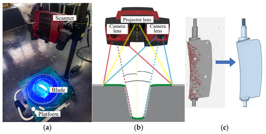
Figure 1.
(a) High-resolution scanner; (b) Working principle of the scanner; (c) Modeling procedure for the IGV blade.
The scanning and modeling of blades capture only their geometric features. These blades are assembled on the shroud and hub following specific positional relationships. The scanner is employed to scan the shroud and hub structures, followed by surface fitting to create their 3D models. Geometric constraint-based virtual assembly of all component models is performed to obtain the 3D model of HPC. To reduce the workload of mesh generation and improve computational efficiency, a single passage, as shown in Figure 2, is extracted to represent the entire nine-stage HPC. For each blade of all stages, 12 cross-sectional planes are uniformly positioned along the blade span to extract contour data from the 3D model as the foundational dataset to enable parametric modeling of the geometric features of the HPC blades. Twelve cross-sections are selected to ensure sufficient spanwise resolution for capturing geometric variations, while avoiding an excessive amount of data that would significantly increase computational cost. Geometric contours of the hub and shroud are captured by marking reference points on the structures.

Figure 2.
Single passage of the nine-stage HPC.
2.2. Parametric Reconstruction of Blade Geometric Deviations
2.2.1. Leading-Edge Erosion
During actual engine operation, erosion phenomena occurring in the HPC include leading-edge erosion, mid-chord erosion, and trailing-edge erosion. To reasonably simplify the problem, the present study focuses exclusively on leading-edge erosion, which represents the most frequently observed erosion mode [8]. To accurately represent the deviations of critical blade geometric features, a developed program, as illustrated in Figure 3, reconstructs the deteriorated geometry of the leading edge. The contour data are first preprocessed, including initial data sorting and outlier processing. The preprocessed data are fitted using the non-uniform rational B-spline (NURBS) method [26]. To perform erosion simulation, a variable leading-edge region, as illustrated in Figure 4, is defined. The leading-edge point A, the trailing-edge point B, and their corresponding chord line L1 are identified on a blade cross-section. The geometric variation range at the leading edge is defined as 1.5% of the chord length, and a line perpendicular to the mean camber line at this location is the segmented line L2.
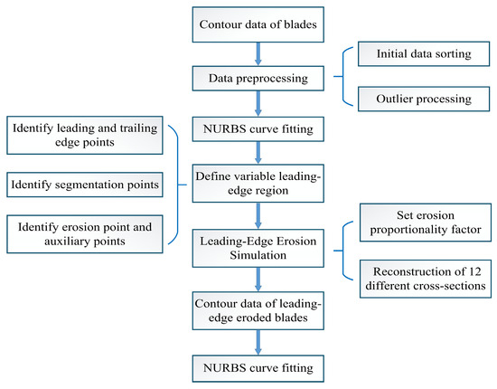
Figure 3.
Parametric reconstruction program.
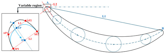
Figure 4.
Variable leading-edge region.
The segmented line divides the blade contour into two regions: the variable leading-edge zone and the non-variable zone. The intersections of the segmented line with the suction-side and pressure-side contours are defined as segmented points SP1 and SP2, while the intersection with the mean camber line is defined as IP. The blue curve represents the eroded leading-edge profile of the blade, and its intersection with the mean camber line defines the erosion point EP. A perpendicular line L3 is drawn at EP on the mean camber line, with the intersection points on either side of the blade designated as auxiliary points AP1 and AP2.
Due to the high complexity of leading-edge erosion during actual engine operation, which typically involves diverse and stochastic erosion morphologies, this paper adopts and improves upon the methodology proposed by Reitz et al. [27]. The leading-edge erosion proportionality factor is introduced to rationally simplify the leading-edge erosion process, thereby ensuring computational tractability while preserving physical relevance. Parametric reconstruction of a deteriorated leading-edge contour is achieved by constructing a control polygon defined by two auxiliary points and two segmented points. Leading-edge erosion is conceptualized as the inward retreat of leading-edge point A along the mean camber line. The proportionality factor is defined as the ratio of the distance that point A moves along the mean camber line towards the intersection point IP to 1.5% of the chord length. quantifies the erosion depth range of the leading edge, and the NURBS method is utilized to fit the deteriorated leading edge. The process iterates until the leading edges of 12 different cross-sections are fully reconstructed.
2.2.2. Surface Roughness and Tip Clearance
Roughness serves as a critical geometric feature for characterizing the surface smoothness of blades and is represented by the equivalent sand-grain roughness [28] in this paper. The parameter exhibits a linear relationship with the mean surface roughness of the contour. According to Koch et al. [29], this relationship for HPC blades is expressed as . In commercial CFD software ANSYS 19.2, smooth wall surfaces are converted into walls with varying roughness levels by modifying the wall function, thereby enabling simulations of different blade surface roughness. In addition, leading-edge erosion can alter blade surface roughness. However, this study simplifies modeling by treating erosion and surface roughness as independent geometric deviations, and the effect of erosion-induced roughness variation is not taken into account.
In CFD simulations, blade tip clearance is determined by measuring the distance from the shroud surface to the cross-section of the blade tip that is parallel to it. This allows direct specification of tip clearance increments to simulate blade tip wear. Additionally, the quality of the mesh generated for the fluid and solid domains significantly determines the accuracy of the simulation results. To ensure effective performance transfer between the HPC stages and control the gradient of computational errors, the mesh in the tip clearance and passage regions requires refinement based on the initially generated mesh.
The HPC 3D model obtained through reverse modeling and virtual assembly is integrated with the parametric reconstruction of blade geometric deviations, enabling the construction of a comprehensive geometric digital model. This model not only stores the original geometric features of the HPC, but also allows customized modifications of parameterized features. The geometric digital model serves as the foundation for subsequent deterioration simulations.
3. Three-Dimensional CFD Simulation
3.1. Automated High-Fidelity Simulation Process
An automated, high-fidelity 3D CFD simulation process is developed to investigate the impact of blade geometric deviations on the HPC aerodynamic performance. The studied HPC consists of nine stages, each containing tens to hundreds of blades. In total, the nine-stage HPC contains 614 rotor blades and 816 stator blades. To reasonably simplify the simulation workflow, it is assumed that each blade within a single passage represents the entire annulus of blades. Therefore, in the CFD simulations, the geometric deviations assigned to different blades within the same stage are identical; however, this does not alter the fact that the simulated configuration remains a complete nine-stage HPC model comprising both rotor and stator blades. The TurboGrid module in ANSYS 19.2 is used to generate the mesh for all blade structures and gas flow passages. ANSYS CFX is employed as the solver for simulations. In the automated simulation process, and are set to 0, while tip clearance is set to the design value to conduct the design point condition simulation. Additionally, the shear stress transport (SST) turbulence model is employed, with the turbulence intensity set to 5%. The isentropic efficiency , pressure ratio , and inlet/outlet mass flow of the HPC are defined as the performance parameters to be monitored in simulations, with the first two defined using the following formulas:
where and denote the total pressure and total temperature at the outlet, respectively, while and denote the values at the inlet. denotes the temperature ratio, and denotes the specific heat ratio of the gas. After completing the preprocessing setup, simulations are performed with an iteration step of 400. To simplify the simulation process, the bleed air used for turbine cooling in the HPC is not considered. Therefore, the inlet and outlet mass flows remain equal. To ensure the accuracy and stability of the simulation results, the convergence criteria require that the root mean square residuals of the momentum, energy, and continuity equations fall below 10−5, and the variations in isentropic efficiency, pressure ratio, and mass flow remain within 0.01%.
A mesh independence study is conducted under the design point operating condition using five different mesh sizes of 5 million, 7 million, 9 million, 11 million, and 13 million cells. As illustrated in Figure 5, when the mesh size exceeds 9 million, both efficiency and pressure ratio exhibit noticeable stabilization. The differences in efficiency and pressure ratio between the 9 million and 13 million mesh sizes are 0.07% and 0.03%, respectively. Considering the simulation accuracy and computational cost, a mesh size of 9 million cells is selected for the CFD simulation. As shown in Figure 6, the mesh of the R1 blade is presented. The overall mesh distribution is relatively uniform, with local refinements applied to the blade surface and tip clearance region. The elements exhibit a regular shape, which ensures the accuracy and stability of subsequent CFD simulations. Figure 7 illustrates the final single-passage HPC simulation domain imported into ANSYS CFX. In the CFD analysis, the prescribed boundary conditions include the total pressure and total temperature at the HPC inlet, as well as the static pressure at the outlet.
Figure 5.
Efficiency and pressure ratio under different mesh sizes.
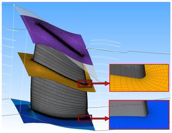
Figure 6.
The mesh of the R1 blade.
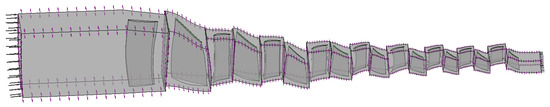
Figure 7.
Single-passage HPC simulation domain.
To obtain the HPC characteristics at the design rotational speed, the outlet static pressure is reduced from the design point of 2520 kPa to 2400 kPa, 2350 kPa, 2100 kPa, and 1100 kPa, respectively, while keeping all other conditions unchanged. The resulting characteristic curves of the HPC are illustrated in Figure 8.
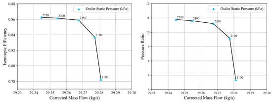
Figure 8.
HPC characteristic curves at the design rotational speed.
3.2. Simulations of Blade Geometric Deviations
The front stages of a multistage axial HPC interact with airflow earlier and have a larger contact area compared to the rear stages, making them more prone to geometric deviations. Considering the computational cost of CFD simulations, this paper investigates three types of geometric features in the IGV and the first-stage rotor blade R1. In simulations, the range of is set between 0 and 0.6, assuming a uniform erosion distribution along all cross-sections. Gilge et al. [30] measured the surface condition of R1 blades of a compressor after 20,000 flight cycles and found that ranged from 0 to 50 μm, with the majority distributed between 7 and 37 μm. The real blade surface cannot be perfectly smooth. However, to investigate the effect of geometric deviation uncertainty on performance, the initial value of is set to 0 μm, thereby covering the widest possible parameter range. Accordingly, the variation range of in simulations of this paper is set to 0~50 μm, while is constrained within 0~1 mm based on the maximum serviceable limit specified in the relevant engine shop maintenance manual. Unlike leading-edge erosion and surface roughness, the variations of R1 blade tip clearance are studied solely, as the IGV blades are stator blades. CFD simulations are performed under five outlet static pressure conditions: 2520 kPa, 2400 kPa, 2350 kPa, 2100 kPa, and 1100 kPa. The results are presented in Figure 9.
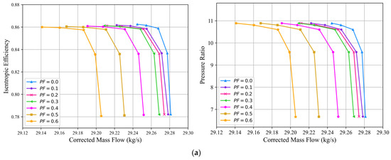
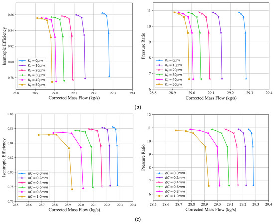
Figure 9.
(a) Simulation results of leading-edge erosion; (b) Simulation results of increased blade surface roughness; (c) Simulation results of increased tip clearance.
Figure 9a illustrates that as the leading-edge erosion of the blades progressively increases, the mass flow within the HPC passages decreases, accompanied by slight reductions in both efficiency and pressure ratio. Under the boundary condition of an outlet static pressure of 2520 kPa, when increases from 0 to 0.6, the HPC mass flow, efficiency, and pressure ratio decrease by only 0.354%, 0.292%, and 0.00826%, respectively. Figure 9b presents the simulation results for blade surface roughness. As increases, the mass flow also decreases, with a greater reduction compared to the impact of leading-edge erosion. The increase in surface roughness enhances the friction between the blade surface and the airflow, leading to boundary layer thickening and a reduction in the effective flow area, thereby causing additional flow losses. Additionally, it is observed that when the blade transitions from a fully smooth state to = 10 μm, the mass flow experiences a significant reduction. The increase in also leads to reductions in pressure ratio and efficiency, with efficiency experiencing a relatively greater decline. As increases, the amplitude of HPC aerodynamic performance degradation gradually decreases. Under the boundary condition of an outlet static pressure of 2520 kPa, when increases from 0 μm to 50 μm, the corresponding decreases in mass flow, efficiency, and pressure ratio are 1.14%, 0.784%, and 0.0845%.
Figure 9c shows the simulation results of R1 blade tip clearance gradually increasing by 1.0 mm from the initial standard value. As the tip clearance increases uniformly, the characteristic curves shift progressively toward the lower-left corner. Compared to leading-edge erosion and increased blade surface roughness, the impact of increased tip clearance on performance is more significant. Under the boundary condition of an outlet static pressure maintained at 2520 kPa, increasing from 0 mm to 1.0 mm results in reductions of 1.95%, 1.33%, and 0.828% in mass flow, efficiency, and pressure ratio.
By examining the velocity field of the HPC simulations, it is observed that an increase in tip clearance intensifies the tip leakage flow in the first three blade stages and enhances the local turbulence near the blade tips. This turbulence interacts with the main flow, ultimately inducing flow separation and tip stall in the first three stages. As leading-edge erosion progressively increases, flow separation also gradually develops along the leading edges of the first three stages. With the progressive increase in either tip clearance or leading-edge erosion, these adverse flow separation phenomena intensify, eventually reducing the effective flow capacity of the HPC and leading to a gradual decrease in mass flow, as shown in Figure 9.
4. Engine Performance Digital Twin Modeling
4.1. 0D Performance Modeling Based on Real Operating Data
OpenMDAO, developed by Gray et al. [31], is an open-source framework for the multidisciplinary analysis, design, and optimization of complex engineering systems. Hendricks et al. [32] developed PyCycle based on the OpenMDAO framework, which is an engine thermodynamic cycle analysis tool. Under identical data and model settings, its results exhibit an error of less than 0.03% compared to the widely used Numerical Propulsion System Simulation (NPSS) [33] model.
For the studied engine, a 0D performance model is developed based on selected modules from pyCycle to analyze performance at both design and off-design conditions. The principle of this model is illustrated in Figure 10. The engine test data at the design rotational speed is selected for design point matching. The model constructs and connects digital modules corresponding to each component of the real engine. Considering the errors introduced by the test bench and the installation effects, the test data first requires correction. The corrected data is then used as input for the performance model, including flight conditions (such as altitude and Mach number), low-pressure spool speed (), high-pressure spool speed (), net thrust (), and combustor exit temperature (). Additionally, the performance parameters of each component, such as efficiency and total pressure loss coefficient, are specified.

Figure 10.
The process of constructing an engine 0D performance model.
The model iteratively adjusts the engine inlet mass flow (), fuel-to-air ratio (), and pressure ratios of the high and low pressure turbines (/) by setting initial values and variation ranges. The iteration continues until both and reach the design targets and the power balance between the high-pressure and low-pressure spools is achieved. The iterative computation is performed using OpenMDAO’s built-in Newton-based nonlinear solver, with a convergence error limit set to 10−8. The relative error between a model’s output data and real operating data is defined as follows:
where denotes output data, and denotes real data. The off-design point calculations proceed if the maximum remains within 1.5%, and the mean of all data remains within 1%. Otherwise, the performance parameters of each component need to be adjusted for re-matching.
The design point-matching process scales the generic component characteristic maps embedded in the performance model to calibrate the model to the real engine. For off-design point matching, the real operating data of the engine are utilized for the calculation. According to the engine control law, off-design matching simulates the throttling characteristics, where the engine thrust is controlled by adjusting the throttle lever position. Therefore, the input real operating data consist of flight conditions and the target net thrust values. Real data from 36 operating points covering the entire in-flight phase were selected and corrected before being imported into the model. The model iterates by setting initial values and variation ranges of , , and until reaches the target value and the power balance between the high-pressure and low-pressure spools is achieved. The maximum between an output data and real data must not exceed 2%, and the mean of all data must remain within 1.5%. Otherwise, the matching process needs to be repeated.
To validate the accuracy of the constructed model, real data from 36 operating points covering the entire in-flight phase, extracted from the same engine cycle, are input into the model for off-design point calculations. The mean of all data for each operating point is illustrated in Figure 11, where the maximum mean is 1.71%, and the average of all mean is 1.23%. Therefore, the developed performance model shows high accuracy and stability, meeting the requirements of engine performance calculations.
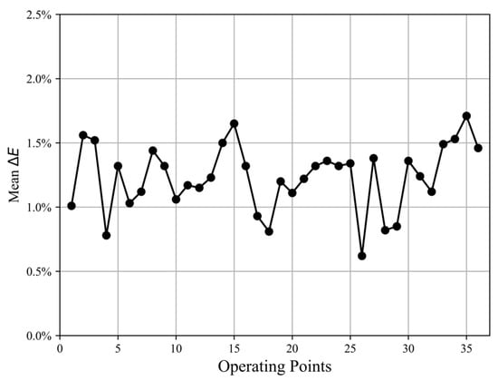
Figure 11.
Mean relative errors between all output data and real operating data.
4.2. Cross-Scale Coupling Method
To investigate the impact of blade geometric deviations on engine performance, it is necessary to couple the HPC aerodynamic performance obtained from CFD simulations with engine performance. This process, which integrates 3D CFD simulations with a 0D performance model, is also referred to as cross-scale performance coupling and is commonly addressed using numerical zooming technologies. These techniques include weak coupling, iterative coupling, and full coupling methods [34]. Among them, the weak coupling method [35] preserves the integrity and stability of the performance model while significantly reducing computational costs compared to the other two methods.
As shown in Figure 12, the weak coupling method is employed by incorporating a developed HPC geometric digital model and a real operating data-based engine performance model. Based on this method, a PDT model is further constructed. Firstly, a 0D performance model is constructed, from which the HPC inlet and outlet boundary conditions are extracted. Based on these boundary conditions, high-fidelity 3D CFD simulations are performed to obtain deterioration characteristic maps. The characteristic maps are scaled and integrated into the performance model, replacing the generic characteristic maps for further degraded performance calculations.

Figure 12.
Cross-scale coupling method and engine PDT modeling.
4.3. PDT Modeling and Validation
The integration of CFD simulations with a performance model ultimately forms an engine PDT model. This model is established based on the thermodynamic principles of the engine cycle, real operating data, and an HPC geometric digital model. It constructs a virtual–physical mapping between the engine’s physical and digital entities. Consequently, the PDT model enables high-precision simulation of various geometric deviations occurring in real engine blades and quantitatively assesses the impact of localized deteriorations on overall engine performance.
The effect of the increase in R1 blade tip clearance on HPC aerodynamic performance is coupled with engine performance using the PDT model. Variations of and specific fuel consumption at different R1 blade tip wear conditions are shown in Figure 13, where solid lines denote the real values in the relevant engine shop maintenance manual, while the dashed lines represent the predicted values calculated using the PDT model. It can be observed that as increases from 0.2 to 0.8 mm, both the and increase. The relative errors between the predicted and real values remain below 5%, indicating that the proposed model exhibits high accuracy and precision.
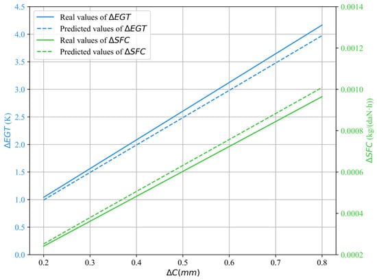
Figure 13.
Variations of and at different R1 blade tip wear conditions.
5. Case Study
5.1. SVR-Based Surrogate Modeling
The geometric deviation of HPC blades during manufacturing and operation is not a single degradation, but a stochastic combination of multiple deterioration types. These deteriorations do not follow deterministic variations but exhibit specific probabilistic distributions. Due to the complex structure of the engine and its unique operating environment, collecting data on blade geometric uncertainty is typically challenging and expensive. As a result, determining the probability distributions of blade geometric deviations is highly difficult [8]. It is assumed that the probability distributions of the three types of geometric deviations studied in this paper follow a normal distribution, as shown in Table 1. Considering that the real blade surface cannot be perfectly smooth, the primary range of is maintained between 10 μm and 50 μm.

Table 1.
Normal distribution of three types of geometric deviation.
A stratified random sampling of three geometric features of the R1 blade is performed using the Latin hypercube sampling (LHS) [11] method to generate 150 samples. These samples are then input into the automated CFD simulation process to obtain HPC performance characteristics. The engine PDT model is applied to derive the engine performance characteristics. A dataset comprising 150 samples is obtained for training and testing the surrogate model.
Support vector regression (SVR) is essentially an extension of support vector machines, and its computational complexity does not depend on the dimensionality of the input space [36]. When handling high-dimensional datasets, SVR-based surrogate models are simpler and exhibit superior generalization capability compared to models based on deep learning or other approaches. Therefore, an SVR-based method is employed in this paper to construct the surrogate model. It maps low-dimensional input features to a high-dimensional feature space using kernel functions and seeks a regression function in this space that tolerates a certain level of error while maintaining model simplicity. Its optimization objective is formulated as follows:
where controls the tolerance for training errors. In total, 80% of the sample data is used as the training set for the SVR model, with the remaining 20% reserved for testing. The radial basis function is selected as the kernel function for the SVR model, and a 5-fold cross-validation is performed to determine the optimal combination of hyperparameters.
The relative errors of the SVR models constructed for predicting the HPC aerodynamic performance and the overall engine performance are evaluated on the test dataset. The relative errors in HPC aerodynamic performance are all within 0.7%, with the majority falling below 0.5%. Similarly, the relative errors in engine performance remain at a low level, all within 0.15%, with most values below 0.13%. Therefore, the developed surrogate model exhibits high accuracy and meets the requirements for high-fidelity and rapid performance prediction.
5.2. Uncertainty Quantification of the Impact of Blade Geometric Deviations
A study is conducted on cases where three types of blade geometric deviation are randomly combined within their respective distribution ranges. A total of 5 million combined samples are generated using the LHS method. These samples are then input into the developed SVR models to compute the performance. The results are collated to quantify the propagation of uncertainty from blade geometric deviations to HPC aerodynamic performance and ultimately to engine performance, as illustrated in Figure 14 and Figure 15. The vertical axes of the figures represent the probability density of the variables, which characterizes the statistical distribution of the variables. The probability density is normalized so that the total area of all histogram bins equals one, thereby representing the relative frequency distribution of the variable values. Consequently, the probability density on the vertical axis is dependent on the range of the variable along the horizontal axis. When the distribution range is narrow, the corresponding probability density becomes high, as in the cases of pressure ratio and isentropic efficiency. The orange curves represent kernel density estimation, which approximates the probability density functions of the samples. And the red lines denote the design point reference values of each performance parameter. The effect of combined geometric deviations leads to performance deterioration, where mass flow, pressure ratio, and efficiency decrease, while and increase.
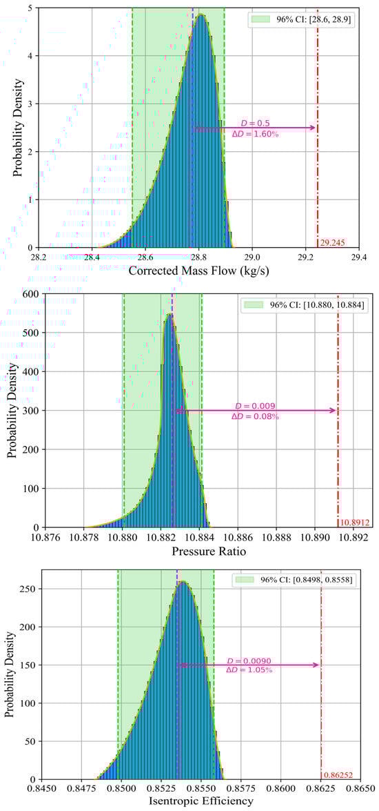
Figure 14.
Impact of blade combined deviation on HPC aerodynamic performance.
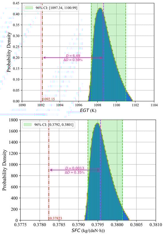
Figure 15.
Impact of blade combined deviation on overall engine performance.
When the degraded HPC performance is coupled into the whole engine model for off-design calculations, this deterioration propagates to the overall cycle. The engine performance model developed conducts off-design calculations by iterating with thrust as the fixed target value, which is elaborated on in detail in Section 4.1. To maintain the same thrust, the combustor must consume more fuel, resulting in a higher combustor exit temperature. Consequently, both the exhaust gas temperature and the specific fuel consumption increase.
The purple lines in the figures indicate the 50th percentile (median). The parameters and represent the absolute and relative distances between the median and reference values. It is observed that of the pressure ratio is 0.08%, which is significantly lower than that of mass flow and efficiency. The pressure ratio exhibits lower sensitivity to the combined geometric deviations compared to the other two parameters. This is consistent with the results of individual simulations for each geometric deviation presented in Section 3.2. Additionally, the of is 0.59%, nearly twice that of , indicating that exhibits higher sensitivity to combined deviations than .
During engine maintenance, standard repair or replacement of deteriorated components is commonly performed to ensure that engine performance meets the operating requirements. To improve maintenance strategies, CBM is implemented to conduct targeted repairs based on the current condition of engines, thereby reducing maintenance costs. Therefore, it is essential to quantify the impact of blade geometric deviations before and after engine blade repair.
In Figure 14 and Figure 15, the green region represents a 96% confidence interval (CI) of the samples, with the left and right green dashed lines corresponding to the 2nd and 98th percentiles. It is assumed that in real operation, the performance requirements dictate that must not exceed 1099 K at a 98% confidence level, and must not exceed 0.3795 kg/(daN·h) at a 98% confidence level. Both fail to meet the performance requirements. Consequently, HPC blade maintenance or replacement should be considered to restore performance.
In this work, only blade tip wear is restored to investigate the effect of deviations after repair. HPC blade tip repair is typically performed using tip filler materials [37]. Due to repair inaccuracies and operating uncertainties, the restored blade tip clearance is not a fixed value but follows a specific probabilistic distribution. The restored tip clearance is assumed to follow a normal distribution with a mean of 0.2 mm and a standard deviation of 0.05 mm, while the other two geometric features remain unchanged. The impact of deviations after repair is quantified, as illustrated in Figure 16. The blue histogram represents the original probability distribution of the performance parameters before repair, while the purple histogram shows the post-repair distribution. The green region denotes the 96% CI of the post-repair distribution. It can be observed that, after repair, remains below 1098.37 K and stays below 0.3795 kg/(daN·h) at a 98% confidence level, both meeting the performance requirements.
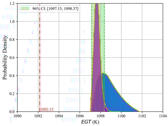
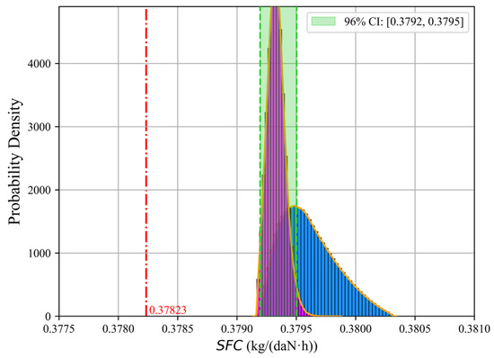
Figure 16.
Impact of blade combined deviation after repair on engine performance.
According to the OEM-recommended maintenance procedures, further and more in-depth repairs on tip clearance or other geometric deviations may still be required in addition to the restoration of blade tip wear. However, the uncertainty quantification results obtained through the PDT model indicate that under the previously assumed maintenance scheme, where only partial restoration of the tip clearance is performed, the overall engine performance already meets operational requirements, eliminating the need for additional blade repairs. Therefore, the uncertainty quantification method based on the engine PDT model enhances the CBM strategy, reducing maintenance costs while providing a more scientific basis for the overall engine performance assessment.
6. Conclusions
This paper presents an uncertainty quantification method for assessing the impact of HPC blade geometric deviations. Simulations of three types of deviation—leading-edge erosion, increased surface roughness, and tip wear—are conducted based on an HPC geometric digital model. An engine performance digital twin (PDT) model is developed and validated to evaluate engine performance. Surrogate models are developed based on SVR to quantify the impact of blade geometric deviations on overall engine performance. The main results of this paper can be summarized as follows:
- In the CFD simulations, the HPC mass flow, efficiency, and pressure ratio decrease as the deviation increases. The increase in tip clearance increment from 0 mm to 1.0 mm exerts the most significant impact on HPC aerodynamic performance. Under the boundary condition of maintaining an outlet static pressure of 2520 kPa, the mass flow, efficiency, and pressure ratio decrease by 1.95%, 1.33%, and 0.828%, respectively. When equivalent sand-grain roughness increases from 0 μm to 50 μm, the corresponding reductions are 1.14%, 0.784%, and 0.0845%. In contrast, an increase in the leading-edge erosion proportionality factor from 0 to 0.6 results in only minor decreases of 0.354%, 0.292%, and 0.00826%.
- The developed engine performance model exhibits high accuracy. Among 36 selected operating points, the maximum mean (relative error) between the model outputs and real operating data is 1.71%, with an average value of 1.23%. By integrating the 0D performance model with the HPC geometric digital model, an engine PDT model is developed. The model is validated by comparing the results of simulating the deviation of R1 blades with the relevant manual data.
- The impact of combined deviation is analyzed by constructing surrogate models. The sensitivity of pressure ratio to combined deviation is lower than that of efficiency and mass flow, with the median of its degraded probability distribution decreasing by only 0.08% relative to the standard design value. EGT exhibits higher sensitivity than SFC, with its median increasing by 0.59%. The engine performance before and after blade tip repair in the CBM scenario is evaluated, demonstrating that the proposed method based on the PDT model improves maintenance strategies and reduces maintenance costs.
In future studies, a more comprehensive geometric digital model can be constructed by incorporating additional blade geometric features, such as stagger angle deviation. Secondly, the proposed method can be further applied to multiple stages of blades beyond the R1 rotor, and different geometric deviations can be set for blades within the same stage to perform multi-passage CFD simulations, which provides a closer representation of real operating conditions. The sensitivity of engine performance to each geometric feature can also be investigated using sensitivity analysis methods. The shop maintenance workscope can be optimized using the PDT model based on the results of sensitivity analysis. Furthermore, further studies can be conducted to inversely allocate performance requirements to blade geometric features, enabling more precise constraints on blade geometric deviations during real engine operation.
Author Contributions
Conceptualization, J.S.; methodology, P.T.; software, P.T.; validation, J.S. and P.T.; formal analysis, J.N.; investigation, J.N.; resources, J.S.; data curation, J.L.; writing—original draft preparation, P.T.; writing—review and editing, P.T.; visualization, J.L.; supervision, Q.L.; project administration, Q.L.; funding acquisition, J.S. All authors have read and agreed to the published version of the manuscript.
Funding
This research was funded by the NSFC & CAAC Joint Research Fund, grant number U2233204.
Data Availability Statement
The original contributions presented in this study are included in the article. Further inquiries can be directed to the corresponding author.
Conflicts of Interest
Author Qin Liu was employed by the company AECC Sichuan Gas Turbine Establishment. The remaining authors declare that the research was conducted in the absence of any commercial or financial relationships that could be construed as a potential conflict of interest.
Abbreviations
The following abbreviations are used in this manuscript:
| CBM | Condition-based maintenance |
| CFD | Computational fluid dynamics |
| CI | Confidence interval |
| EGT | Exhaust gas temperature |
| HPC | High-pressure compressor |
| IGV | Inlet guide vane |
| LHS | Latin hypercube sampling |
| MCS | Monte Carlo simulation |
| MRO | Maintenance, repair, and overhaul |
| NIPC | Non-intrusive polynomial chaos |
| NPSS | Numerical propulsion system simulation |
| NURBS | Non-uniform rational B-spline |
| OEM | Original equipment manufacturer |
| PDT | Performance digital twin |
| SFC | Specific fuel consumption |
| SST | Shear stress transport |
| SVR | Support vector regression |
| 0D | Zero-dimensional |
| 3D | Three-dimensional |
| Fuel-to-air ratio | |
| Net thrust | |
| High-pressure turbine pressure ratio | |
| Equivalent sand-grain roughness | |
| Low-pressure turbine pressure ratio | |
| Low-pressure spool speed | |
| High-pressure spool speed | |
| Erosion proportionality factor | |
| Fan inlet total pressure | |
| HPC outlet static pressure | |
| Combustor exit temperature | |
| HPC inlet total temperature | |
| Engine inlet mass flow | |
| Isentropic efficiency | |
| Total-to-total pressure ratio | |
| Total-to-total temperature ratio | |
| Tip clearance increments | |
| Relative error |
References
- Javed, A.; Pecnik, R.; Van Buijtenen, J.P. Optimization of a centrifugal compressor impeller for robustness to manufacturing uncertainties. ASME J. Eng. Gas Turbines Power 2016, 138, 112101. [Google Scholar] [CrossRef]
- Marx, J.; Städing, J.; Reitz, G.; Friedrichs, J. Investigation and analysis of deterioration in high pressure compressors due to operation. CEAS Aeronaut. J. 2014, 5, 515–525. [Google Scholar] [CrossRef]
- Wang, J.Y.; Yang, H.L.; Zhou, K.; Wei, J.; Wen, M.; Zheng, X. Performance dispersion control of a multistage compressor based on precise identification of critical features. Aerosp. Sci. Technol. 2022, 129, 107845. [Google Scholar] [CrossRef]
- Denkena, B.; Nyhuis, P.; Bergmann, B.; Nübel, N.; Lucht, T. Towards an autonomous maintenance, repair and overhaul process: Exemplary holistic data management approach for the regeneration of aero-engine blades. Procedia Manuf. 2019, 40, 77–82. [Google Scholar] [CrossRef]
- Ahmad, R.; Kamaruddin, S. An overview of time-based and condition-based maintenance in industrial application. Comput. Ind. Eng. 2012, 63, 135–149. [Google Scholar] [CrossRef]
- Labib, A.W. A decision analysis model for maintenance policy selection using a CMMS. J. Qual. Maint. Eng. 2004, 10, 191–202. [Google Scholar] [CrossRef]
- Montomoli, F. Uncertainty Quantification in Computational Fluid Dynamics and Aircraft Engines; Springer: Cham, Switzerland, 2015; pp. 1–3. [Google Scholar] [CrossRef]
- Wang, J.; Zheng, X. Review of geometric uncertainty quantification in gas turbines. ASME J. Eng. Gas Turbines Power 2020, 142, 070801. [Google Scholar] [CrossRef]
- Hu, X.; Chen, X.; Parks, G.T.; Yao, W. Review of improved Monte Carlo methods in uncertainty-based design optimization for aerospace vehicles. Prog. Aerosp. Sci. 2016, 86, 20–27. [Google Scholar] [CrossRef]
- Garzon, V.E.; Darmofal, D.L. Impact of geometric variability on axial compressor performance. ASME J. Turbomach. 2003, 125, 692–703. [Google Scholar] [CrossRef]
- Lange, A.; Voigt, M.; Vogeler, K.; Schrapp, H.; Johann, E.; Gümmer, V. Probabilistic CFD simulation of a high-pressure compressor stage taking manufacturing variability into account. In Proceedings of the ASME Turbo Expo 2010: Power for Land, Sea, and Air, Glasgow, UK, 14–18 June 2010; ASME: New York, NY, USA, 2010; pp. 617–628. [Google Scholar] [CrossRef]
- Giebmanns, A.; Schnell, R.; Werner-Spatz, C. A method for efficient performance prediction for fan and compressor stages with degraded blades. In Proceedings of the ASME Turbo Expo 2015: Turbine Technical Conference and Exposition, Montreal, QC, Canada, 15–19 June 2015; ASME: New York, NY, USA, 2015; p. V02AT37A006. [Google Scholar] [CrossRef]
- Xu, S.; Zhang, Q.; Wang, D.; Huang, X. Uncertainty Quantification of Compressor Map Using the Monte Carlo Approach Accelerated by an Adjoint-Based Nonlinear Method. Aerospace 2023, 10, 280. [Google Scholar] [CrossRef]
- Gong, Y.; Zhang, J.; Xu, D.; Huang, Y. Quantile-based optimization under uncertainties for complex engineering structures using an active learning basis-adaptive PC-Kriging model. Chin. J. Aeronaut. 2025, 38, 103197. [Google Scholar] [CrossRef]
- Shahpar, S.; Seshadri, P.; Parks, G. Leakage uncertainties in compressors: The case of Rotor 37. J. Propuls. Power 2015, 31, 456–466. [Google Scholar] [CrossRef]
- Wang, J.; Wang, B.; Yang, H.; Sun, Z.; Zhou, K.; Zheng, X. Compressor geometric uncertainty quantification under conditions from near choke to near stall. Chin. J. Aeronaut. 2023, 36, 16–29. [Google Scholar] [CrossRef]
- Zhang, H.; Yue, K.; Zhang, Y. Geometric Optimization of Coanda Jet Chamber Fins via Response Surface Methodology. Aerospace 2025, 12, 571. [Google Scholar] [CrossRef]
- Shi, M.; Lv, L.; Sun, W.; Song, X. A multi-fidelity surrogate model based on support vector regression. Struct. Multidiscip. Optim. 2020, 61, 2363–2375. [Google Scholar] [CrossRef]
- He, X.; Zheng, X. Performance improvement of transonic centrifugal compressors by optimization of complex three-dimensional features. Proc. Inst. Mech. Eng. G J. Aerosp. Eng. 2017, 231, 2723–2738. [Google Scholar] [CrossRef]
- Ma, C.; Gao, L.; Cai, Y.; Li, R. Robust optimization design of compressor blade considering machining error. In Proceedings of the ASME Turbo Expo 2017: Turbomachinery Technical Conference and Exposition, Charlotte, NC, USA, 26–30 June 2017; ASME: New York, NY, USA, 2017; p. V02CT47A003. [Google Scholar] [CrossRef]
- Kraft, J.; Sethi, V.; Singh, R. Optimization of aero gas turbine maintenance using advanced simulation and diagnostic methods. ASME J. Eng. Gas Turbines Power 2014, 136, 111601. [Google Scholar] [CrossRef]
- Reitz, G.; Friedrichs, J. Impact of front- and rear-stage high pressure compressor deterioration on jet engine performance. Int. J. Turbomach. Propuls. Power 2018, 3, 15. [Google Scholar] [CrossRef]
- Grieves, M.; Vickers, J. Digital twin: Mitigating unpredictable, undesirable emergent behavior in complex systems. In Transdisciplinary Perspectives on Complex Systems; Kahlen, J., Flumerfelt, S., Alves, A., Eds.; Springer: Cham, Switzerland, 2017; pp. 85–113. [Google Scholar] [CrossRef]
- Hu, M.; He, Y.; Lin, X.; Lu, Z.; Jiang, Z.; Ma, B. Digital twin model of gas turbine and its application in warning of performance fault. Chin. J. Aeronaut. 2023, 36, 449–470. [Google Scholar] [CrossRef]
- Xiong, M.L.; Wang, H.W.; Fu, Q.; Xu, Y. Digital twin-driven aero-engine intelligent predictive maintenance. Int. J. Adv. Manuf. Technol. 2021, 114, 3751–3761. [Google Scholar] [CrossRef]
- Gálvez, A.; Iglesias, A. Particle swarm optimization for non-uniform rational B-spline surface reconstruction from clouds of 3D data points. Inf. Sci. 2012, 192, 174–192. [Google Scholar] [CrossRef]
- Reitz, G.; Kellersmann, A.; Schlange, S.; Friedrichs, J. Comparison of sensitivities to geometrical properties of front and aft high pressure compressor stages. CEAS Aeronaut. J. 2018, 9, 135–146. [Google Scholar] [CrossRef]
- Nikuradse, J. Law of flows in rough pipes. NACA Tech. Memo. 1933, 1292. Available online: https://digital.library.unt.edu/ark%3a/67531/metadc63009/ (accessed on 20 August 2025).
- Koch, C.C.; Smith, L.H. Loss sources and magnitudes in axial-flow compressors. ASME J. Eng. Gas Turbines Power 1976, 98, 411–424. [Google Scholar] [CrossRef]
- Gilge, P.; Kellersmann, A.; Friedrichs, J.; Seume, J.R. Surface roughness of real operationally used compressor blade and blisk. Proc. Inst. Mech. Eng. G J. Aerosp. Eng. 2019, 233, 5321–5330. [Google Scholar] [CrossRef]
- Gray, J.S.; Hwang, J.T.; Martins, J.R.R.A.; Moore, K.T.; Naylor, B.A. OpenMDAO: An open-source framework for multidisciplinary design, analysis, and optimization. Struct. Multidiscip. Optim. 2019, 59, 1075–1104. [Google Scholar] [CrossRef]
- Hendricks, E.S.; Gray, J.S. pyCycle: A Tool for Efficient Optimization of Gas Turbine Engine Cycles. Aerospace 2019, 6, 87. [Google Scholar] [CrossRef]
- Claus, R.W.; Evans, A.L.; Lytle, J.K.; Nichols, L. Numerical propulsion system simulation. Comput. Syst. Eng. 1991, 2, 357–364. [Google Scholar] [CrossRef]
- Turner, M.G.; Reed, J.A.; Ryder, R.; Veres, J.P. Multi-fidelity simulation of a turbofan engine with results zoomed into mini-maps for a zero-D cycle simulation. In Proceedings of the ASME Turbo Expo 2004: Power for Land, Sea, and Air, Vienna, Austria, 14–17 June 2004; ASME: New York, NY, USA, 2004; pp. 219–230. [Google Scholar] [CrossRef]
- Pachidis, V.; Pilidis, P.; Templalexis, I.; Barbosa, J.B.; Nantua, N. A de-coupled approach to component high-fidelity analysis using computational fluid dynamics. Proc. Inst. Mech. Eng. G J. Aerosp. Eng. 2007, 221, 105–113. [Google Scholar] [CrossRef]
- Awad, M.; Khanna, R. Support vector regression. In Efficient Learning Machines; Apress: Berkeley, CA, USA, 2015; pp. 154–156. [Google Scholar] [CrossRef]
- Denkena, B.; Boess, V.; Nespor, D.; Floeter, F.; Rust, F. Engine blade regeneration: A literature review on common technologies in terms of machining. Int. J. Adv. Manuf. Technol. 2015, 81, 917–924. [Google Scholar] [CrossRef]
Disclaimer/Publisher’s Note: The statements, opinions and data contained in all publications are solely those of the individual author(s) and contributor(s) and not of MDPI and/or the editor(s). MDPI and/or the editor(s) disclaim responsibility for any injury to people or property resulting from any ideas, methods, instructions or products referred to in the content. |
© 2025 by the authors. Licensee MDPI, Basel, Switzerland. This article is an open access article distributed under the terms and conditions of the Creative Commons Attribution (CC BY) license (https://creativecommons.org/licenses/by/4.0/).