Model-Based Tracking in a Space-Simulated Environment Using the General Loss Function

Abstract

The increasing demand for on-orbit servicing (OOS), such as satellite life extension and space debris removal, has highlighted the need for research into precise relative navigation between space objects. Model-based tracking (MBT) was applied using the imaging data for relative navigation, incorporating SPNv2 (Spacecraft Pose Network v2) for an initial pose estimation. Furthermore, the performance of General Loss was evaluated by applying it during the model tracking processes and comparing it with seven other robust M-estimators, including Tukey, Welsch, and Huber. The simulations were conducted in a ROS–Gazebo environment that emulated a rendezvous with the International Space Station (ISS). Six approach profiles were generated by pairing three mutually different conic-section apertures with two attitude modes—boresight locked on the ISS versus boresight fixed on the inertial origin—producing six distinct spiral trajectories that bring the chaser from 500 m to 100 m along the depth axis of the camera. General Loss achieved superior estimation accuracy in most profiles. Thus, the proposed algorithm, which integrates General Loss into the MBT-based relative navigation framework, provides robust and stable performance in the presence of diverse residual distributions and outliers. In the few instances where it did not yield the very best results, the initial error arose from matching virtual edges—generated according to the sample weight distribution—to the actual edges in the image frame; notably, by the end of the simulation, when the camera reached a depth of approximately 100 m, these errors were substantially reduced. Thus, the proposed algorithm, which integrates General Loss into the MBT-based relative navigation framework, provides robust and stable performance in the presence of diverse residual distributions and outliers.

1. Introduction

Technologies for satellite life extension, servicing, and the recovery of malfunctioning spacecraft have become increasingly important with the commercialization of low Earth orbit (LEO) satellites and the rapid deployment of large satellite constellations. At the same time, the accumulation of space debris in orbit has significantly heightened the risk of collisions between satellites, drawing global attention to on-orbit servicing (OOS) technologies aimed at mitigating these threats [1].

OOS encompasses a broad range of operations, including the repair of existing satellites, refueling, attitude stabilization, health monitoring, component replacement, and the active removal of space debris. Successfully executing these tasks requires high-precision relative navigation capabilities to ensure safe and accurate interaction with target objects in space [2].

Various sensor-based approaches have been investigated for relative navigation between satellites, including Light Detection and Ranging (LiDAR) [3,4], Radio Detection and Ranging (RADAR), and vision sensors [5,6]. Among these, vision-based image-processing techniques have advantages in hardware compactness, energy efficiency, and information density. Model-Based Tracking (MBT) [7] has attracted attention as a practical approach for structured objects because it enables a real-time estimation of the relative position and orientation by aligning features extracted from images with a known Computer-Aided Design (CAD) model of the target object.

Despite these advantages, MBT requires an accurate initial pose, making the estimation highly sensitive to initialization. Moreover, performance degradation can occur under real space conditions because of varying illumination, surface reflections, sensor noise, and outliers in the image data. Outliers can significantly distort the pose estimation results, which necessitates robust methods to mitigate their impact. Error minimization techniques based on M-estimators have been widely used to address this, utilizing various weighting functions to suppress the influence of outliers during optimization [8,9].

This study utilized Spacecraft Pose Network v2 (SPNv2) [10], a convolutional neural network-based model, solely for initial pose estimation in MBT, owing to its relatively high computational cost compared to the subsequent MBT process. After initialization, robustness against dynamically varying noise was enhanced using the General Loss function [11], which continuously adapts its shape via a single parameter within an iteratively reweighted least squares (IRLS) tracking framework.

Building upon this combination of SPNv2-based initialization and IRLS tracking with reweighting explicitly governed by the General Loss function, this study proposes an extended MBT framework. General Loss dynamically adjusts its shape through a single parameter α, enabling continuous adaptation to varying noise characteristics. This approach not only mitigates the dependency on accurate initial poses but also improves robustness under dynamically changing weighting conditions, without relying on fixed weighting functions that suppress the influence of outliers [8,9].

To validate the proposed method, this study conducted a comparative evaluation of the General Loss function against seven representative M-estimators, including Tukey [8,12], Welsch [9,13], and Huber [14]. A rendezvous profile with the International Space Station (ISS) was simulated in a ROS–Gazebo environment. The relative position and orientation estimation accuracies of each estimator were quantified using the Root Mean Square Error (RMSE) metric.

The results validate the proposed approach, demonstrating that embedding General Loss in the IRLS loop of MBT delivers robust, high-precision relative navigation and shows strong promise for future on-orbit servicing (OOS) missions.

2. Methodology

2.1. Model-Based Tracking Framework Overview

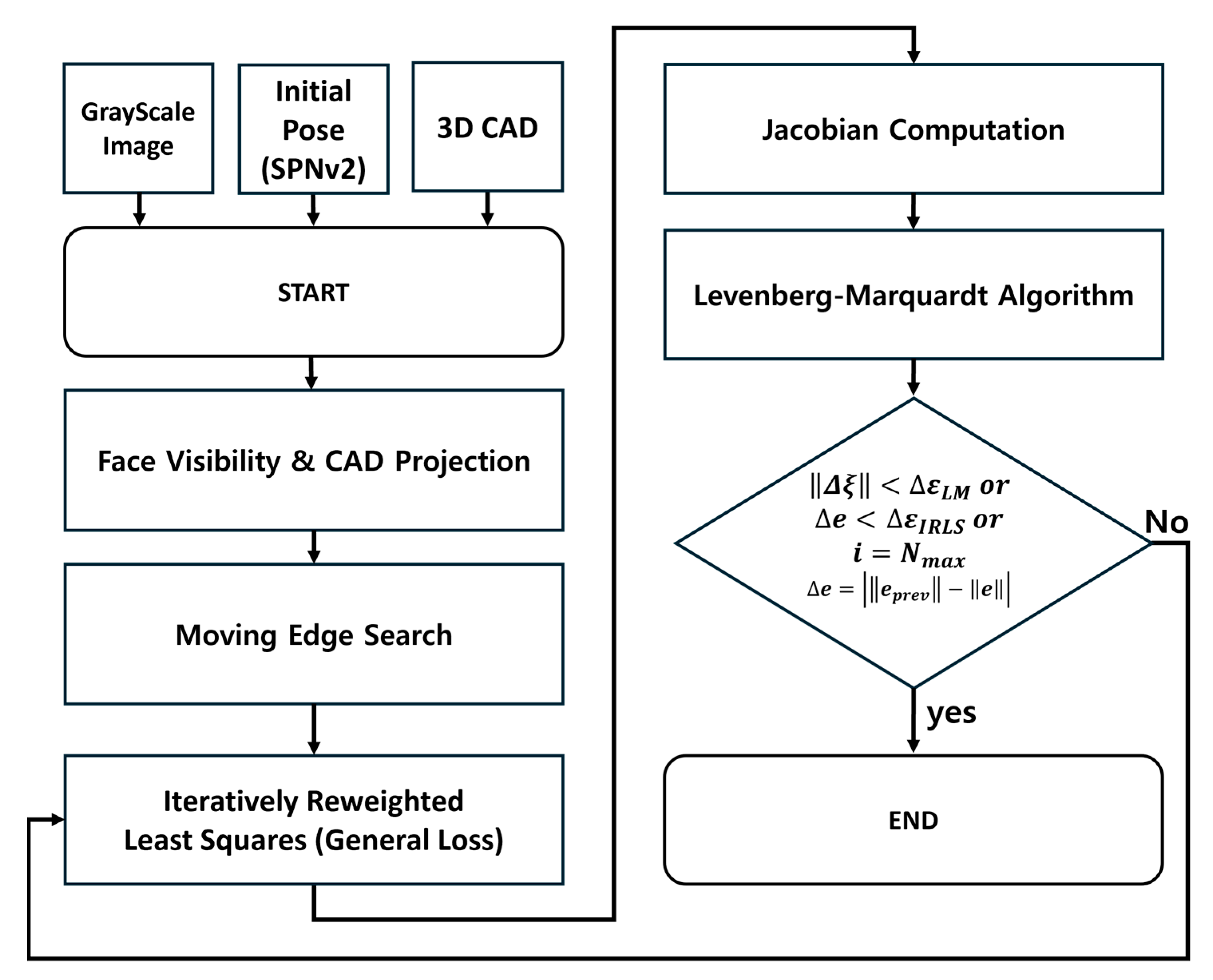
To enhance reproducibility and provide a comprehensive understanding of the overall system, this section outlines the complete pose tracking pipeline used in this study. As illustrated in Figure 1, the proposed framework consists of two main modules:

• Initial pose estimation using SPNv2
• IRLS based optimization using a General Loss function.

Given an input image and a corresponding 3D CAD model of the target spacecraft, the system first estimates an initial relative pose using the proposed SPNv2-based initialization, which provides robust and accurate starting conditions for tracking. Following this initialization, the MBT pipeline begins with the face visibility determination and CAD projection to identify the visible contours of the model in the current view. A moving edge search is then performed to associate these projected contours with the observed image edges.

In each iteration, the process begins with IRLS optimization using the proposed General Loss function to compute robust weights for the current correspondences, ensuring robustness against outliers. The weighted Jacobian matrix is then computed based on these weights, and the Levenberg–Marquardt (LM) algorithm is applied to update the pose estimate. This iterative process continues until the predefined convergence criteria, which combine LM tolerance, IRLS residual variation, and iteration limits, are met. Initial pose estimation was performed using SPNv2 (available at: https://github.com/tpark94/spnv2, accessed on 2 July 2025), and the subsequent MBT was implemented with ViSP 3.6.1 (Inria, Rennes, France).

2.2. Model-Based Tracking

MBT projects a simplified CAD model onto the image plane based on the provided initial position and orientation. The relative pose is then estimated by minimizing the error ($∆$) between the observed features ($s^{*}$) from the camera and the corresponding features ($s$) projected from the CAD model. This error minimization can be performed using either the least squares approach or robust M-estimators.

In this study, the feature set is defined as comprising the 16 solar panel edges of the ISS model. These edges are projected from the CAD model and serve as the reference contours for measurement. For each edge, a set of moving edge sites is initialized by uniformly sampling points along the projected contour in the image plane.

Each site stores its 2D location, normal direction, and depth. The local image gradient is then sampled along the contour’s normal direction to build a 1D gradient profile, and the position of maximum gradient magnitude is detected as the observed feature position (${s_i}^{*}$). The error between the projected and observed contours can be mathematically expressed as

$$∆=\sum _{i=1}^N{(s_i\left(r\right)-{s_i}^{*})}^2=\sum _{i=1}^N{\left(p{r}_{\xi }\right(r,{{}^{o}P}_i)-{s_i}^{*})}^2,$$

(1)

where $\xi$ denotes the intrinsic camera parameters, and $r$ represents the position and orientation of the camera. The projection model $p{r}_{\xi }\left(r,{{}^{o}P}_i\right)$ is defined by $\xi$ and $r$, and $N$ is the number of considered features. The confidence-weighted error for each feature is expressed by defining the residual as follows:

$$e=D(s\left(r\right)-s^{*}),$$

(2)

where $D$ is a diagonal weighting matrix; $D=diag({\omega }_1, {\omega }_2,\cdots {\omega }_i)$, with each $w_i$ reflecting the confidence of $i$^th feature calculated as follows:

$${\omega }_i={\displaystyle \frac{\psi \left(u_i\right)}{u_i}},$$

(3)

where ${\omega }_i$ denotes the normalized residual defined as $u_i=Median\left(r\right)$, and $\psi \left(u_i\right)$ is the influence function derived from the M-estimator. The projection error for that site is then calculated as the signed distance along the contour normal between the model-projected position $s_i\left(r\right)$ and the detected edge position ${s_i}^{*}$. This ensures that the residual specifically measures displacement orthogonal to the model edge, making it robust to tangential misalignments. The variation of the residual with respect to the position and orientation can be expressed as

$$\dot{e}={\displaystyle \frac{\partial e}{\partial s}}{\displaystyle \frac{\partial s}{\partial r}}{\displaystyle \frac{\partial r}{\partial t}}=D{L}_{s}v,$$

(4)

where $L_s\in {\mathbb{R}}^{N\times 6}$ denotes the interaction matrix, and $v\in {\mathbb{R}}^6$ represents the velocity of the virtual camera. Assuming an exponential decay model of the error $\dot{e}= \lambda e$, the control law is derived as

$$v=-\lambda {\left(\widehat{D}\widehat{L_s}\right)}^{+}D(s\left(r\right)-s^{*}),$$

(5)

where ${\left(\widehat{D}\widehat{L_s}\right)}^{+}$ represents the pseudo-inverse of the weighted interaction matrix $\left(\widehat{D}\widehat{L_s}\right)$, which is updated at each iteration based on the current weights and estimated depths. The virtual velocity $v$, corresponding to the differential update of the pose $r$, converges or the iteration and reaches a maximum number of iterations. At this point, the relative pose between the model and the camera is determined. 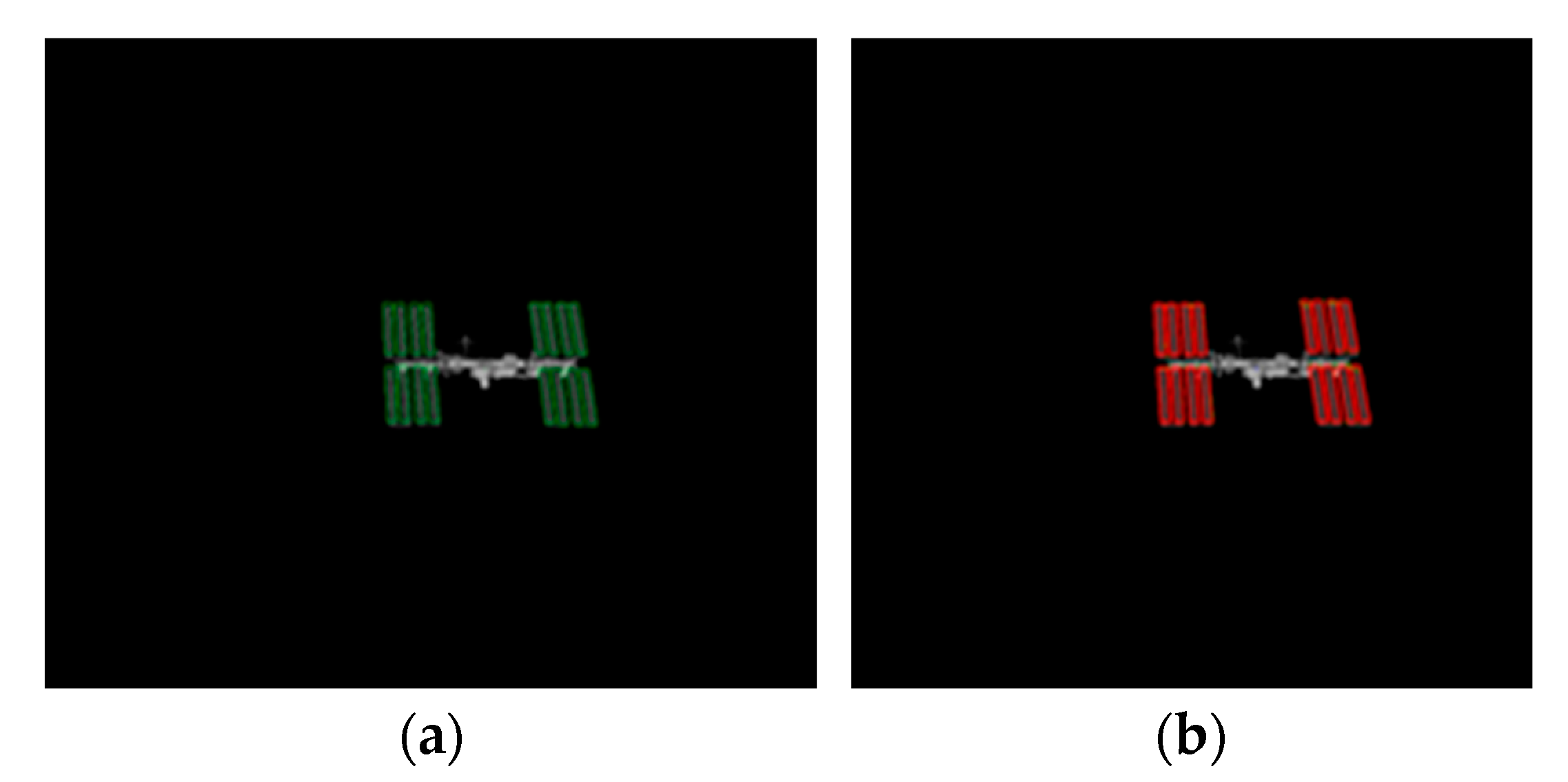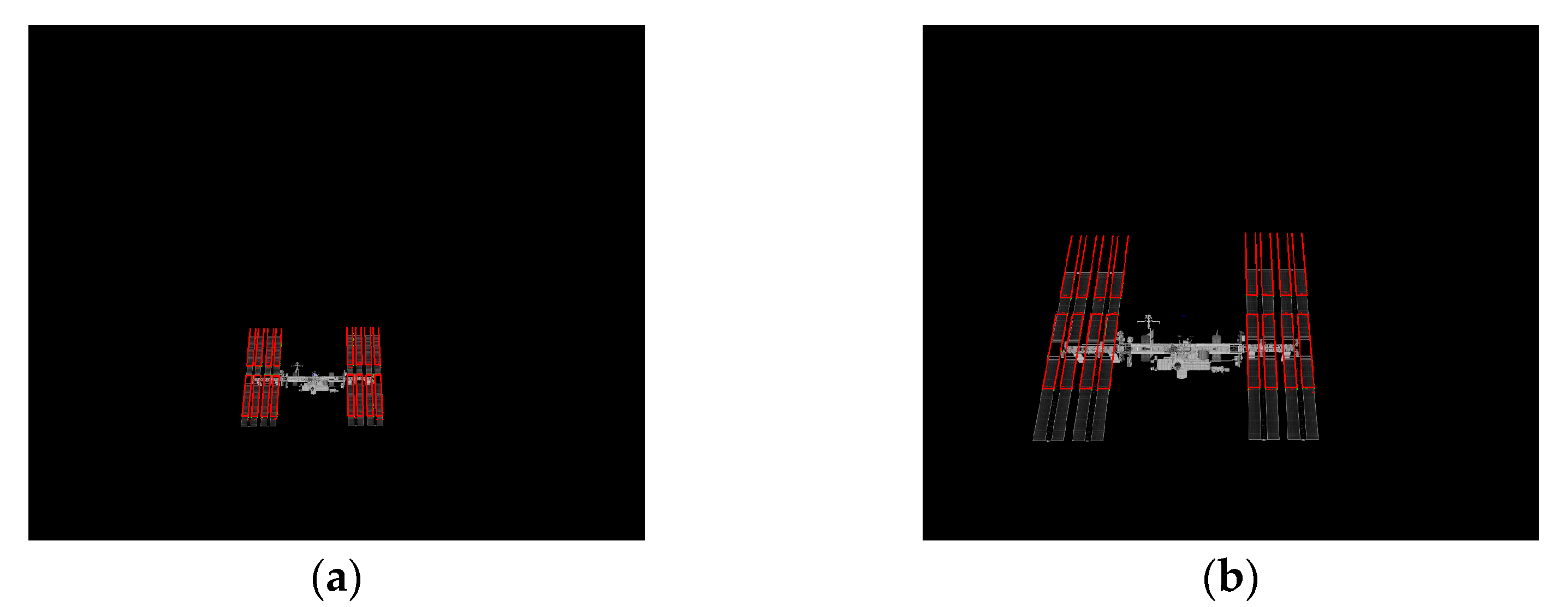Figure 2a presents the projected initial pose $r$ used to initialize MBT, and Figure 2b shows the target-tracking and relative-navigation solution produced by MBT.

2.3. SPNv2

SPNv2 is a deep learning model designed to regress the six-DoF (Degrees of Freedom) pose from a single RGB image. The model adopted a Bi-directional Feature Pyramid Network (BiFPN) based on EfficientDet-D3 as its backbone architecture as a two-stage network that combines a heatmap head and a pose regression head.

The Heatmap Head predicts the 2D bounding box and keypoint heatmaps of the satellite from multi-scale feature maps. It generates outputs that include the object presence probability, bounding box classification, and bounding box regression. Subsequently, the Pose Regression Head extracts the region of interest (ROI) and directly regresses the rotation quaternion and translation vector.

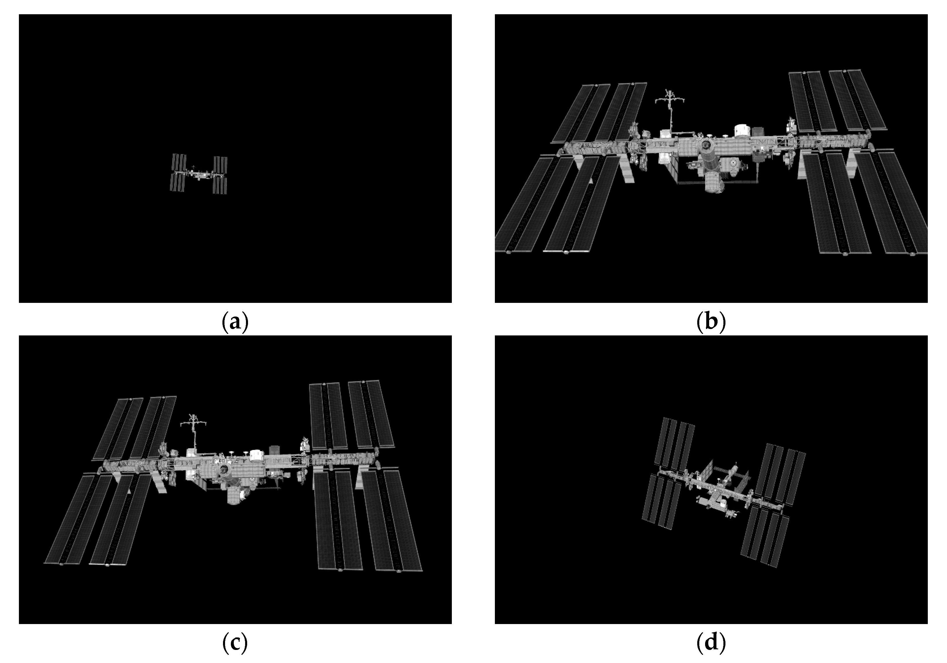
A dataset of 20,000 synthetic images was generated in a ROS–Gazebo environment under a simulated ISS rendezvous profile, with positional constraints 100 m $\le$ x $\le$ 1000 m and angular constraints $\left|\theta \right|<30°, \left|\varphi \right|<30°$. Angle offsets proportional to the relative distance along the x-axis of the camera coordinate frame were introduced to enhance training data diversity.

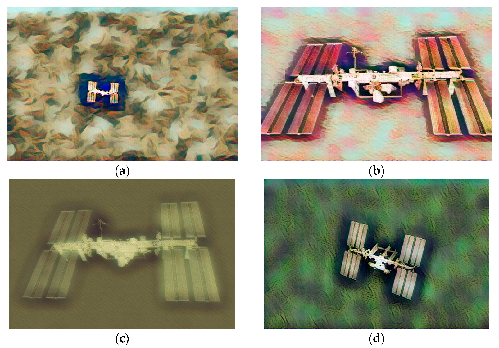
In addition, randomized visual styles were applied to the dataset, with augmented samples used during training at a 50% probability. This approach enhances the robustness of the model across varying visual environments [15]. Figure 3 shows the raw dataset collected from the simulation, while Figure 4 shows the augmented dataset with random visual styles.

2.4. Robust M-Estimator and General Loss Function

The least squares method is commonly used to estimate the position and orientation. On the other hand, this method is sensitive to outliers that significantly degrade the accuracy in the presence of noise or erroneously detected feature points. This study adopted robust estimation methods known as M-estimators to overcome this limitation. M-estimators suppress the influence of outliers by reducing the associated weights as the magnitude of the residual increases, providing stable and accurate estimates.

Specifically, this study used the General Loss function, a generalized robust loss formulation capable of continuously adapting its shape through a single parameter. This adaptability allows the algorithm to maintain robustness against dynamically varying noise conditions. The performance of the proposed MBT framework with General Loss was compared with seven representative robust estimators: Tukey, Welsch, Huber, Cauchy, Talwar, Logistic, and Andrews. The mathematical definitions and characteristics of these estimators are summarized as follows.

2.4.1. Tukey

The Tukey estimator eliminates the influence of outliers by assigning a zero weight to residuals that exceed a predefined threshold c. The loss function and corresponding weight function of the Tukey estimator are defined using Equations (6) and (7):

$$\rho \left(r\right)=\left\{\begin{array}{ll}{\displaystyle \frac{c^2}{6}}\left[1-{\left(1-{\displaystyle \frac{r^2}{c^2}}\right)}^3\right],& \left|r\right|\le c\\ {\displaystyle \frac{c^2}{6}},& \left|r\right|>c\end{array}\right.,$$

(6)

$$\omega \left(r\right)=\left\{\begin{array}{ll}\left[{\left(1-{\displaystyle \frac{r^2}{c^2}}\right)}^3\right],& \left|r\right|\le c\\ 0,& \left|r\right|>c\end{array}\right.,$$

(7)

Although it offers excellent robustness to outliers, the Tukey estimator is sensitive to the initial estimate. An inaccurate initial pose may lead to convergence issues during optimization.

2.4.2. Welsch

The Welsch estimator suppresses the influence of outliers by exponentially decreasing the weight as the residual magnitude increases. The loss function and corresponding weight function of the Welsch estimator are defined as Equations (8) and (9):

$$\rho \left(r\right)={\displaystyle \frac{c^2}{2}}[1-\mathrm{e}\mathrm{x}\mathrm{p}(-{\displaystyle \frac{r^2}{c^2}})],$$

(8)

$$\omega \left(r\right)=\exp \left(-{\displaystyle \frac{r^2}{c^2}}\right).$$

(9)

Compared to the Tukey estimator, the Welsch estimator handles outliers more moderately and generally offers better convergence stability. Nevertheless, its robustness to such outliers is relatively lower than that of the Tukey estimator because it assigns attenuated weights to extreme outliers rather than zero weights.

2.4.3. Huber

The Huber estimator applies the L2 loss for small residuals and switches to an L1 loss for large residuals, providing a balanced trade-off between estimation accuracy and robustness. Equations (10) and (11) express the loss function and the corresponding weight function of the Huber estimator.

$$\rho \left(r\right)=\left\{\begin{array}{ll}{\displaystyle \frac{1}{2}}{r}^2,& \left|r\right|\le c\\ c\left|r\right|-{\displaystyle \frac{1}{2}}{c}^2,& \left|r\right|>c\end{array}\right.,$$

(10)

$$\omega \left(r\right)=\left\{\begin{array}{ll}1,& \left|r\right|\le c\\ {\displaystyle \frac{c}{\left|r\right|}},& \left|r\right|>c\end{array}\right..$$

(11)

The Huber estimator is computationally efficient and offers stable convergence compared to other estimators. On the other hand, its ability to handle extreme outliers is inferior to that of the Tukey and Welsch estimators.

2.4.4. Cauchy

The Cauchy estimator applies a logarithmic loss function based on the magnitude of the residuals, moderately suppressing the influence of outliers. Although it retains small non-zero weights even for extreme values, minimizing information loss, it does not eliminate the effects of very large outliers. The loss function and corresponding weight function of the Cauchy estimator are defined as Equations (12) and (13):

$$\rho \left(r\right)={\displaystyle \frac{c^2}{2}}\ln (1+{({\displaystyle \frac{r}{c}})}^2),$$

(12)

$$\omega \left(r\right)={\displaystyle \frac{1}{1+{\left(\frac{r}{c}\right)}^2}},$$

(13)

where $c$ is the scale parameter, and the weighting for each residual is determined by the slope of the influence function $\rho \left(r\right)$ [16].

2.4.5. Talwar

The Talwar estimator [17] applies an L2 loss only when the absolute value of the residual is below a certain threshold. Residuals exceeding this threshold are assigned a constant loss value, effectively setting their weights to zero. Although this approach strongly suppresses extreme outliers, it can also eliminate some inliers depending on the choice of the threshold. The loss function and corresponding weight function of the Talwar estimator are defined as Equations (14) and (15).

$$\rho \left(r\right)=\left\{\begin{array}{c}{\displaystyle \frac{1}{2}}{r}^2, \left|r\right|\le c\\ {\displaystyle \frac{1}{2}}{c}^2, \left|r\right|>c\end{array}\right.,$$

(14)

$$\omega \left(r\right)=\left\{\begin{array}{c}1, \left|r\right|\le c\\ 0, \left|r\right|>c\end{array}\right..$$

(15)

2.4.6. Logistic

The Logistic estimator suppresses outliers by increasing the loss in a sigmoid-shaped manner based on the magnitude of the residual. The estimator exhibits high convergence stability owing to its smooth influence function $\psi$. It is more robust than the Huber estimator, while being more moderate in behavior than the Tukey estimator. The loss function and corresponding weight function of the Logistic estimator are defined as Equations (16) and (17). The weight is given by dividing the influence function $\psi \left(r\right)$ by $r$, specifically ${\displaystyle \frac{\tanh (r/c)}{r/c}}$ [18]

$$\rho \left(r\right)=c^2\ln \left(\cosh \right(r/c\left)\right),$$

(16)

$$\omega \left(r\right)={\displaystyle \frac{\tanh (r/c)}{r/c}}.$$

(17)

2.4.7. Andrews

The Andrews estimator smoothly increases the loss using a sinusoidal function within a bounded interval and assigns a zero weight outside this range, completely rejecting extreme outliers. Its non-convex shape offers strong robustness against outliers, but it is more prone to convergence issues such as entrapment in local minima. The loss function and corresponding weight function of the Andrews estimator are defined as Equations (18) and (19) [19]:

$$\rho \left(r\right)=\left\{\begin{array}{ll}{\displaystyle \frac{c^2}{2}}[1-\cos (r/c)],& \left|r\right|\le c\\ {\displaystyle \frac{c^2}{2}}[1-\cos \pi ],& \left|r\right|>c\end{array}\right.,$$

(18)

$$\omega \left(r\right)=\left\{\begin{array}{ll}{\displaystyle \frac{\sin (r/c)}{(r/c)}},& \left|r\right|\le c\\ 0,& \left|r\right|>c\end{array}\right..$$

(19)

2.4.8. General Loss

The General Loss is a robust estimation method that continuously adapts the shape of the loss function based on the residual. Traditional M-estimators, such as Huber and Tukey, use fixed-form loss functions to suppress the influence of outliers. Nevertheless, these fixed functions may not yield optimal performance under varying noise conditions because of their limited adaptability.

In contrast, the General Loss offers a generalized formulation that can smoothly and continuously transition between different loss function shapes using a single parameter. Specifically, it features an adaptive structure in which the loss behavior is adjusted automatically based on the magnitude and distribution of residuals, as controlled by the parameter. The loss function and corresponding weight function of the General Loss are defined in Equations (20) and (21):

$$\rho \left(r,\alpha ,c\right)=\left\{\begin{array}{ll}{\displaystyle \frac{1}{2}}{(r/c)}^2,& if \alpha =2\\ \log \left({\displaystyle \frac{1}{2}}{\left(r/c\right)}^2+1\right),& if \alpha =0\\ 1-\exp \left(-{\displaystyle \frac{1}{2}}{\left(r/c\right)}^2\right),& if \alpha =-\infty \\ {\displaystyle \frac{\left|\alpha -2\right|}{\alpha }}\left[{({\displaystyle \frac{{\left(r/c\right)}^2}{\left|\alpha -2\right|}}+1)}^{{\displaystyle \frac{\alpha }{2}}}-1\right],& otherwise\end{array}\right.,$$

(20)

$$\omega \left(r,\alpha ,c\right)=\left\{\begin{array}{ll}{\displaystyle \frac{1}{c^2}},& if \alpha =2\\ {\displaystyle \frac{2}{r^2+2c^2}},& if \alpha =0\\ {\displaystyle \frac{1}{c^2}}\exp \left(-{\displaystyle \frac{1}{2}}{\left(r/c\right)}^2\right),& if \alpha =-\infty \\ {\displaystyle \frac{1}{c^2}}\left[\left({({\displaystyle \frac{{\left(r/c\right)}^2}{\left|\alpha -2\right|}}+1)}^{\alpha /2-1}\right)\right],& otherwise\end{array}\right.,$$

(21)

where $r$ denotes the residual at each data point; $\alpha$ is a shape-controlling parameter that determines the form of the loss function, and $c$ is a scale parameter that normalizes the residual magnitude.

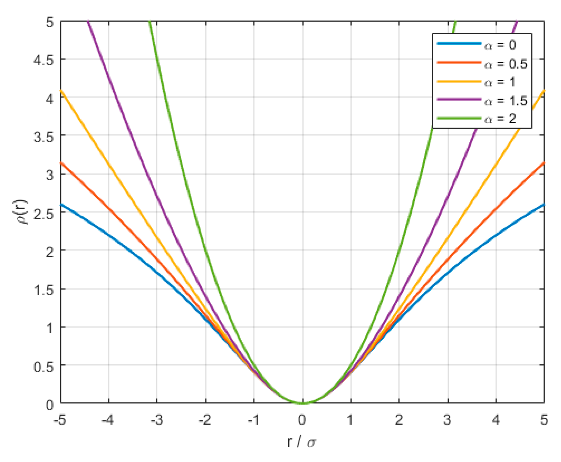
The General Loss function continuously adapts its form based on the residual distribution, determined by a shape-controlling parameter and a scale parameter. The function smoothly transitions among various well-known loss forms, such as the L2 loss ($\alpha =2$), Charbonnier loss ($\alpha =1$), Cauchy loss ($\alpha =0$), and Geman–McClure loss ($\alpha =-2$). The adaptive nature of General Loss provides flexibility in balancing robustness to outliers and the estimation efficiency across diverse noise environments, making it particularly suitable for the relative navigation tasks presented in this study.

The range of $\alpha$ is constrained to [0, 2]. In the original General Loss paper, the adaptation of $\alpha$ was performed through gradient descent over the total loss, implementing an optimization-based adaptive framework. This study adopted a heuristic update strategy based on the difference between the current median residual $u=Median\left(r\right)$ and the previous median value $u_{prev}=Median\left(r_{prev}\right)$ to reduce computational complexity. A gain coefficient $\lambda$ was introduced to modulate this difference, resulting in the update rule defined in Equation (22). Specially, a small change in the median residual leads to a large gain coefficient, allowing rapid adaptation of $\alpha$. On the other hand, a large change, which may reflect instability in the residual distribution, results in a conservative update. Equation (23) defines a candidate ${\alpha }_{cand}$ value that decreases as the residual becomes more outlier-dominated, and Equation (24) blends the old and candidate $\alpha$ using the $\lambda$ to yield a smooth and stable update. Figure 5 presents the loss function of General Loss for different $\alpha$ values. Furthermore, the coefficient used in Equations (23) and (24) is designed such that the value of $\alpha$ remains within the interval [0, 2], ensuring stable behavior throughout the estimation process:

$$\lambda \left(r\right)=\left\{\begin{array}{ll}{\lambda }_{max},& \left|u-u_{prev}\right|\le {\tau }_{low }\\ {\lambda }_{min},& \left|u-u_{prev}\right|\ge {\tau }_{high}\\ {\displaystyle \frac{{\lambda }_{min}+{\lambda }_{max}}{2}},& otherwise\end{array}\right.$$

(22)

$${\alpha }_{cand}=-\kappa +\kappa \times \mathrm{m}\mathrm{i}\mathrm{n}(1,{\displaystyle \frac{\sigma }{u_i}}),$$

(23)

$${\alpha }_{new}=\left(1-\lambda \right)\times {\alpha }_{old}+\lambda \times {\alpha }_{cand}.$$

(24)

where ${\lambda }_{min}$ and ${\lambda }_{max}$ denote the lower and upper bounds of the gain coefficient, ${\tau }_{high}$ and ${\tau }_{low}$ are threshold values that determine the sensitivity to changes in the residual median, $\kappa$ is a scale parameter that normalizes the residual magnitude, $\sigma$ denotes the estimated scale of the residual, and $u$ and $u_{prev}$ represent the current and previous median absolute residuals, respectively, and are used to assess temporal changes in the residual distribution for adaptive $\alpha$ update.

The detailed procedure for adapting $\alpha$ within the IRLS loop is summarized in Algorithm 1 as pseudocode. This pseudocode outlines the computation of residuals, normalization, influence function weighting, and the adaptive update of $\alpha$ based on the current residual distribution.

Algorithm 1 is Pseudocode of the IRLS-based pose refinement algorithm using General Loss.

Algorithm 1: IRLS-based pose refinement algorithm using General Loss

Inputs: image $I$, CAD model $M$, camera intrinsic $K$, initial pose $T_0$ (from SPNv2)

Hyperparameters: scale $c$, thresholds ${\tau }_{low}$, ${\tau }_{high}$, bounds of the gain coefficient ${\lambda }_{min}$, ${\lambda }_{max}$, LM damping ${\mu }_0$, max iteration number $N_{max}$, IRLS/LM tolerances ${\epsilon }_{IRLS}$, ${\epsilon }_{LM}$, mapping constant $\kappa$, small constant $\epsilon$

Outputs: refined pose $\widehat{T}$

Initialize  $T$$\leftarrow T_0$, $\alpha$$\leftarrow {\alpha }_0$$\in [0, 2], \mu$$\leftarrow {\mu }_0$$, i$ ← 0.

repeat

Project M with T, determine face visibility, and perform moving edge search to obtain correspondences and residuals {$r_k$}.

Compute residual vector $e$$\leftarrow [r_1,r_2, \dots , r_n{]}^{\mathrm{T}}$

Compute the median residual $u$$\leftarrow Median\left(\left|r_k\right|\right)$

$\sigma$$\leftarrow 1.4826 \times median\left(\left|\left|r_k\right|-u\right|\right)$

$\mathsf{\Delta }u$$\leftarrow \left|u-u_{prev}\right|$

$\mathrm{Select} \lambda$$\mathrm{based} \mathrm{on} \mathsf{\Delta }u$:

$\mathbf{If} \mathsf{\Delta }u\ge {\tau }_{high}$$\mathrm{then} \lambda$$\leftarrow {\lambda }_{min}$

$\mathbf{Else} \mathbf{if} \mathsf{\Delta }u\le {\tau }_{low}$$\mathrm{then} \lambda$$\leftarrow {\lambda }_{max}$

$\mathbf{Else} \lambda$$\leftarrow {(\lambda }_{min}+{\lambda }_{max})/2$

${\alpha }_{cand}$$\leftarrow -\kappa +\kappa \times \mathrm{m}\mathrm{i}\mathrm{n}(1,{\displaystyle \frac{\sigma }{u+\epsilon }})$

$\alpha$$\leftarrow \left(1-\lambda \right)\times {\alpha }_{old}+\lambda \times {\alpha }_{cand}$, $\mathrm{clip} \alpha$$\mathrm{to} \left[0, 2\right].$

Compute weights:

$\mathbf{Let} r$$:= \left|r_k\right|$

$\mathbf{if} \alpha =2$$: {\mathsf{\omega }}_{\mathrm{k}} \leftarrow 1/c^2$

else if  $\alpha =0$$: {\mathsf{\omega }}_{\mathrm{k}} \leftarrow 2/{(r}^2+2c^2)$

else:  ${\mathsf{\omega }}_{\mathrm{k}} \leftarrow 1/c^2\left[\left({{\left(r/c\right)}^2/\left(\left|\alpha -2\right|\right)+1)}^{\alpha /2-1}\right)\right]$

$\omega$$diag\left(\left\{{\mathsf{\omega }}_{\mathrm{k}}\right\}\right)$

$e_{prev}$$\leftarrow e$

$\mathbf{Solve} (\left(L^{T}WL+\mu I\right)\mathsf{\Delta }\xi =-L^{T}We$

$\mathbf{Update} T$$\leftarrow \mathrm{e}\mathrm{x}\mathrm{p}\left(\mathsf{\Delta }\xi \right)T$

$i$$\leftarrow i+1$

$u_{prev}$$\leftarrow u$

Adapt μ based on the LM gain ratio rule.

$\mathbf{until} (‖\mathsf{\Delta }\xi ‖ < {\epsilon }_{LM}$$\mathrm{and} \left|‖e_{prev}‖-‖e‖\right|$$<$${\epsilon }_{IRLS}$$) \mathrm{or} i \ge N_{max}$

$\mathbf{return} \widehat{T}$$\leftarrow T$

2.5. Simulation

Simulation Environment

The simulation was conducted in the ROS–Gazebo environment using the 3D model of the ISS provided by NASA. The camera parameters used in the simulation are summarized as follows: focal length parameters, $f_x=f_x=$2463.7618 pixels, and principal point parameters, $\left(c_x, c_y\right)=\left(1224, 1024\right)$ pixels. The major specifications of the simulation environment and the system configuration are summarized in

Table 1. Simulation environment and system specification.

Component	Specification
Operating System	Ubuntu 20.04 LTS
ROS version	ROS Noetic
Gazebo Version	Gazebo 11 (classic)
CPU	13th Gen Intel(R) Core (TM) i5-13600KF (20 CPUs) @ 3.5 GHz
RAM	32 GB DDR4 RAM
GPU	NVIDIA GeForce RTX 3060 Ti

.

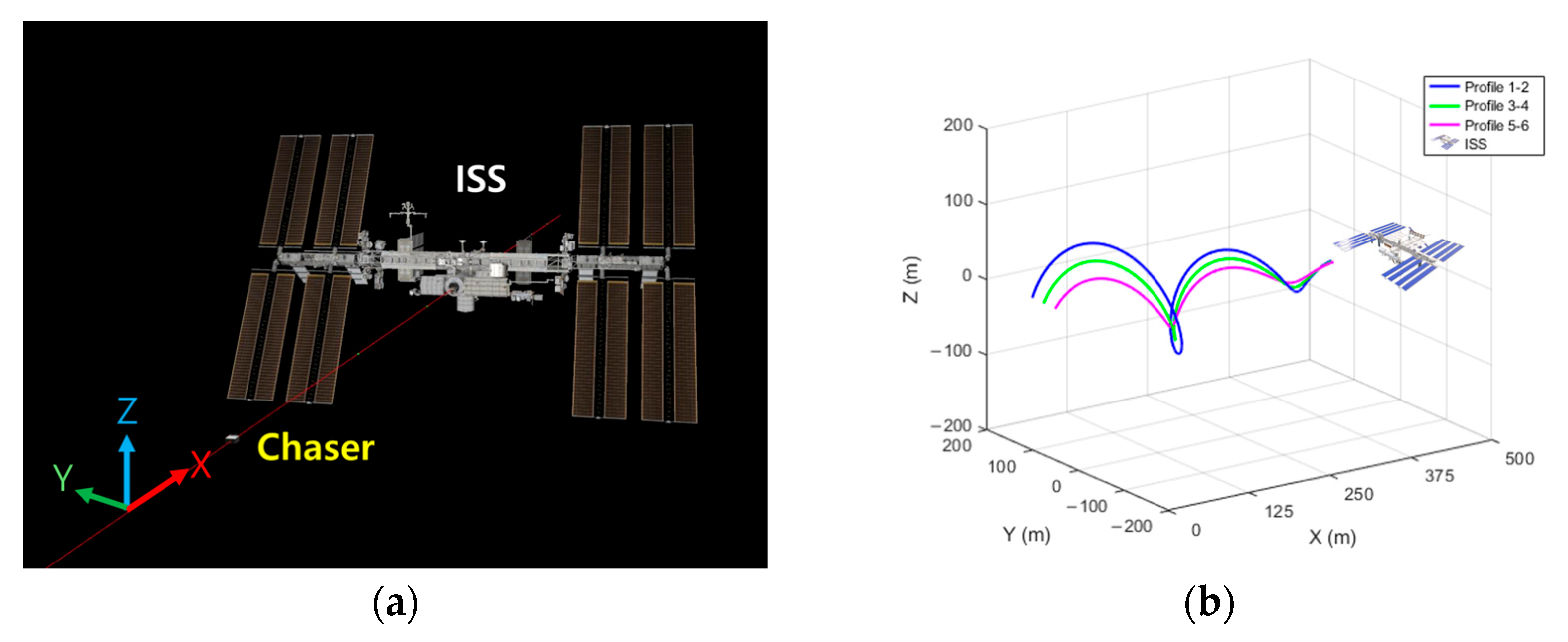
The rendezvous maneuver was simulated by generating a randomized approach corridor and defining a trajectory within this corridor. All data followed the coordinate system shown in Figure 6a, where the ISS and the chaser are initially separated by a relative distance of 500 m along the x-axis, converging gradually toward 100 m. The positions of the y- and z-axes converge simultaneously from an initial radial offset of 100 m.

The effectiveness of General Loss relative to other robust M-estimators was evaluated under various conditions by comparing the MBT-based relative navigation performance across these six profiles. Figure 6a shows the simulation environment and coordinate frames, and Figure 6b presents the trajectory within the approach corridor. To examine the effects of initial estimation errors on the performance of each M-estimator, the initial pose estimates for MBT in each profile were obtained using SPNv2, with a 10° offset applied to the roll axis in profiles 2, 4, and 6.

Table 2. Initial pose average performance error and computation time in heatmap head.

Profile	Average Transitional Error (m)	Average Rotational Error (°)	Offset Applied in Roll Axis (°)	Comp. Time (ms)
1	2.9925	1.4598	0	359.5416
2	1.8098	0.7841	10.0000	346.6957
3	1.9670	1.1674	0	371.7196
4	2.6679	1.1431	10.0000	359.9026
5	2.1564	1.2725	0	355.2330
6	3.2379	1.9091	10.0000	365.7469

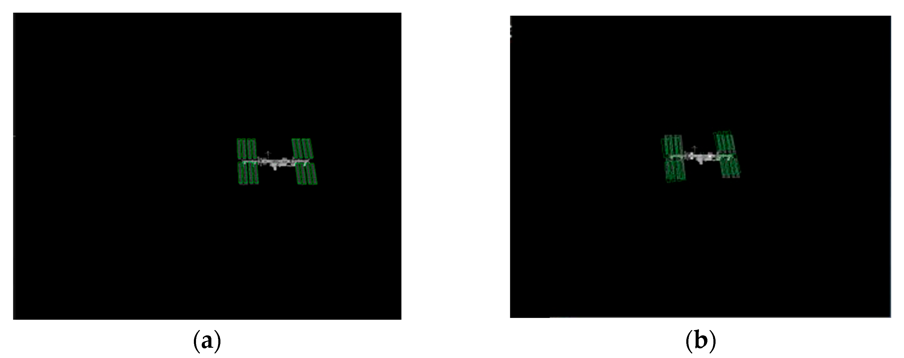
lists the initial position and orientation estimation errors, the applied roll-axis offsets, and the computational time per frame. Figure 7a (profile 1) and Figure 7b (profile 2) show the virtual object models generated from these initial poses.

3. Results

Eight M-estimators (Tukey, Welsch, General Loss, Huber, Cauchy, Talwar, Logistic, and Andrews) were applied as weight functions in the MBT framework. Each M-estimator was used independently per frame, with its corresponding weight function applied to the residuals of that frame. The RMSE was calculated for the position (x, y, z) and orientation (roll, pitch, yaw) over the entire simulation interval, and the computation time per frame was also recorded. The RMSE is defined as follows:

$$RMSE= \sqrt{{\displaystyle \frac{1}{N}}\sum _{i=1}^N{({\widehat{x}}_i-x_i)}^2}$$

(25)

where ${\widehat{x}}_i$ denotes the MBT result, $x_i$ is the ground truth from the simulation, and N is the number of frames. The quantitative results for the entire simulation are presented in

Table 3. RMSE comparison for different M-estimators.

Profile	Weight Function	X (m)	Y (m)	Z (m)	Roll (°)	Pitch (°)	Yaw (°)	Comp. Time (ms)
1	Tukey	1.2327	0.3331	1.4434	0.9307	0.6850	0.8736	26.0755
	Welsch	2.7803	0.2735	4.1141	0.4692	0.3484	0.6705	219.9172
	General Loss	1.0133	0.2606	0.8554	0.3197	0.1805	0.6423	51.0111
	Huber	11.3065	0.3652	18.9850	1.2308	1.0278	2.2931	22.8028
	Cauchy	10.8957	0.3139	17.6180	0.9315	0.6855	1.3773	23.1106
	Talwar	9.7236	0.2836	15.8932	0.5800	0.3414	1.2219	114.7814
	Logistics	13.3429	0.3581	22.0929	1.0344	0.6963	1.0600	143.7517
	Andrews	4.8204	0.3052	7.6722	0.6553	0.5458	0.8617	201.8872
2	Tukey	3.2834	0.5772	4.8830	0.9264	1.7462	2.3079	47.6320
	Welsch	32.8498	23.8333	20.4763	25.0590	13.4518	14.6890	131.3563
	General Loss	4.1985	0.8343	2.4089	1.6920	2.1959	8.9432	56.4875
	Huber	3.7175	0.6503	5.6228	1.0921	2.1573	2.4817	49.8701
	Cauchy	14.7651	2.7015	23.1841	10.7946	7.1007	8.1635	47.3436
	Talwar	24.9902	12.0284	22.0884	9.1846	12.4593	11.4128	94.8042
	Logistics	35.0387	13.9796	30.1389	10.0129	4.6314	13.3272	111.6470
	Andrews	7.3270	4.2215	28.5147	6.1261	7.4520	26.2343	148.7342
3	Tukey	22.2080	1.6978	26.0214	7.5338	4.4717	3.0293	42.0290
	Welsch	17.2112	2.8353	10.9646	14.1623	8.6561	2.6448	223.0419
	General Loss	2.9090	0.3649	0.5905	0.7289	0.4317	0.9193	57.3002
	Huber	19.5186	1.7629	20.9429	7.8593	4.8501	3.4778	43.8880
	Cauchy	26.3641	2.7987	27.0357	13.1464	7.9963	5.1306	42.7596
	Talwar	14.7287	2.4648	8.3352	12.0308	7.3875	2.4346	133.0470
	Logistics	20.7527	4.6151	26.4212	11.2802	7.6271	10.5475	117.6526
	Andrews	20.5869	2.7355	18.0224	13.9113	8.4737	4.016	183.8680
4	Tukey	3.4164	0.8699	1.2292	1.4513	2.5635	4.5983	45.0068
	Welsch	22.0958	17.0129	21.7938	23.03660	12.6191	7.2774	147.8993
	General Loss	4.7912	0.7891	2.0805	2.9494	2.1345	11.2655	56.5872
	Huber	1.3870	0.6188	1.4028	1.5918	2.2937	3.2513	45.5638
	Cauchy	12.1865	3.8447	27.3168	12.5484	7.4562	8.5393	42.1546
	Talwar	14.3056	1.6535	24.3372	3.0644	2.5219	16.3444	103.9845
	Logistics	44.3892	13.4083	34.7487	11.4368	7.6841	15.9215	73.6647
	Andrews	15.9835	4.6074	18.3252	6.5031	7.1975	6.9754	149.5166
5	Tukey	1.0286	0.1435	0.7169	0.2171	0.1621	0.5679	45.4978
	Welsch	0.9948	0.1353	0.7334	0.2082	0.1435	0.4808	207.1718
	General Loss	0.9703	0.1417	0.6347	0.2655	0.1550	0.7000	57.1750
	Huber	11.8357	0.1966	20.0664	1.0241	0.6346	1.1398	43.2750
	Cauchy	12.2700	0.2251	20.2882	1.0828	0.6417	1.5925	43.5649
	Talwar	0.7767	0.1433	0.3322	0.2655	0.1172	1.1036	130.3296
	Logistics	12.7829	0.2150	21.1862	1.2395	0.7977	1.2570	131.3062
	Andrews	1.0515	0.1409	0.7023	0.2104	0.1544	0.5272	149.9439
6	Tukey	6.3060	0.6249	5.2951	1.8122	1.6739	5.8356	47.1019
	Welsch	18.9992	14.0850	23.4471	27.5073	5.3186	10.3394	124.5430
	General Loss	5.2132	0.4000	6.8740	1.5183	1.7240	3.4539	56.7912
	Huber	19.3726	1.2834	23.4333	2.0536	2.0739	6.5240	43.3594
	Cauchy	*	*	*	*	*	*	*
	Talwar	22.0010	6.7870	15.8319	11.5521	2.3085	19.6245	85.8963
	Logistics	13.9365	15.9323	22.6834	27.06880	1.2972	16.1419	75.3147
	Andrews	23.2401	2.4612	17.9198	7.9015	3.8553	21.0676	124.4626

*—indicates a failure in MBT execution.

, whereas the errors at the final simulation frame are provided in

Table A1. Errors at the final simulation frame comparison for different M-estimators.

Profile	Weight Function	X (m)	Y (m)	Z (m)	Roll (°)	Pitch (°)	Yaw (°)
1	Tukey	0.74010	0.0239	0.7651	0.0999	0.0011	0.1055
	Welsch	5.6150	0.0172	9.2040	0.1060	0.0064	0.0731
	General Loss	0.7312	0.0227	0.7529	0.1045	0.0057	0.1052
	Huber	5.1924	0.0184	8.4697	0.0971	0.0021	0.0769
	Cauchy	4.6676	0.0130	7.5593	0.0607	0.0439	0.0863
	Talwar	3.9788	0.0225	6.3670	0.1226	0.0097	0.0732
	Logistics	16.7833	0.5326	29.0767	1.0234	0.5797	1.1070
	Andrews	4.2481	0.0108	6.8407	0.0565	0.0503	0.0750
2	Tukey	3.9676	0.3823	6.3754	0.0604	0.0036	0.0385
	Welsch	106.5176	70.5598	38.7842	32.7787	37.9078	3.3088
	General Loss	0.7779	0.0640	0.7571	0.1356	0.0133	0.1299
	Huber	4.2578	0.4237	6.8632	0.0302	0.0271	0.0211
	Cauchy	19.8306	4.4658	32.3416	6.2607	0.2356	5.8139
	Talwar	21.0223	25.4760	36.8768	18.4730	25.8168	3.5451
	Logistics	28.9112	17.1464	37.3725	3.4853	2.4522	0.5054
	Andrews	0.9473	9.4385	32.6857	7.5496	16.8196	25.2803
3	Tukey	25.8128	0.4211	38.5114	1.9792	1.1563	0.0083
	Welsch	17.6987	1.1984	22.5738	4.0558	2.8475	0.5664
	General Loss	0.3756	0.0089	0.1783	0.0840	0.0114	0.0900
	Huber	21.3331	0.4897	30.3766	2.5245	1.4080	0.4713
	Cauchy	28.0725	0.9245	38.9784	4.3721	2.4982	0.0206
	Talwar	13.2498	0.9663	15.9837	3.8448	2.3542	0.0705
	Logistics	18.5877	5.4220	35.9508	0.7390	0.1146	0.6989
	Andrews	20.5317	0.7383	27.7392	5.5315	3.6272	0.3826
4	Tukey	0.7421	0.05000	0.7628	0.0568	0.0017	0.0712
	Welsch	32.4753	37.7126	21.4503	37.5584	16.1321	18.0444
	General Loss	0.3776	0.0213	0.1271	0.0584	0.0025	0.0709
	Huber	0.7444	0.0503	0.7643	0.0525	0.0021	0.0753
	Cauchy	22.9829	6.8123	39.719	7.3009	4.3486	0.1514
	Talwar	17.2672	0.8550	29.5501	0.7476	0.4421	0.0519
	Logistics	34.6128	13.1422	51.3944	12.6050	11.8133	9.1999
	Andrews	13.3889	8.4248	25.0302	6.9955	11.1389	5.6602
5	Tukey	0.7438	0.0023	0.8016	0.0871	0.0081	0.0861
	Welsch	0.7398	0.0019	0.7961	0.0887	0.0169	0.0886
	General Loss	0.7392	0.0020	0.7935	0.0911	0.0109	0.0888
	Huber	17.5011	0.3541	30.1260	1.5821	1.0349	0.0447
	Cauchy	17.1347	0.4324	29.2902	1.4592	0.9477	0.1523
	Talwar	0.3777	0.0037	0.1640	0.0716	0.0217	0.0841
	Logistics	17.5659	0.4233	30.0221	1.5115	0.9693	0.1764
	Andrews	0.7423	0.0018	0.7962	0.0942	0.0119	0.0856
6	Tukey	5.2127	0.4362	7.7069	0.4965	0.3864	1.2377
	Welsch	15.6906	25.6821	23.3464	34.1111	19.8029	15.4952
	General Loss	0.7808	0.0493	0.7621	0.1251	0.0124	0.1611
	Huber	20.8212	1.4030	30.4295	0.7468	0.6659	0.3376
	Cauchy	*	*	*	*	*	*
	Talwar	11.4093	9.6091	25.3414	21.6496	1.0768	10.5320
	Logistics	7.5772	25.4088	21.5149	42.6180	0.7144	17.4631
	Andrews	25.3291	2.9467	29.5635	11.6640	4.9784	14.0505

*—indicates a failure in MBT execution.

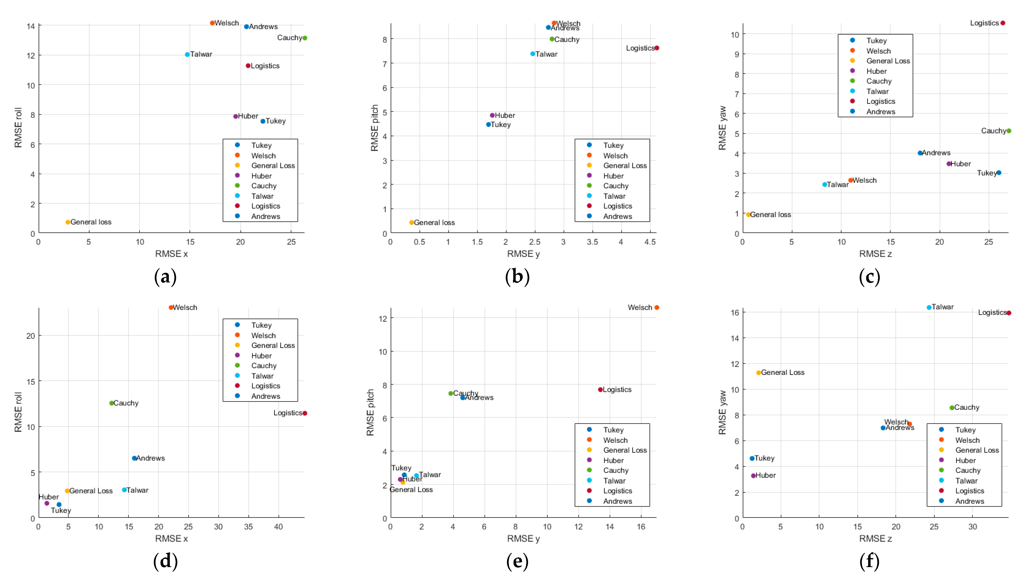
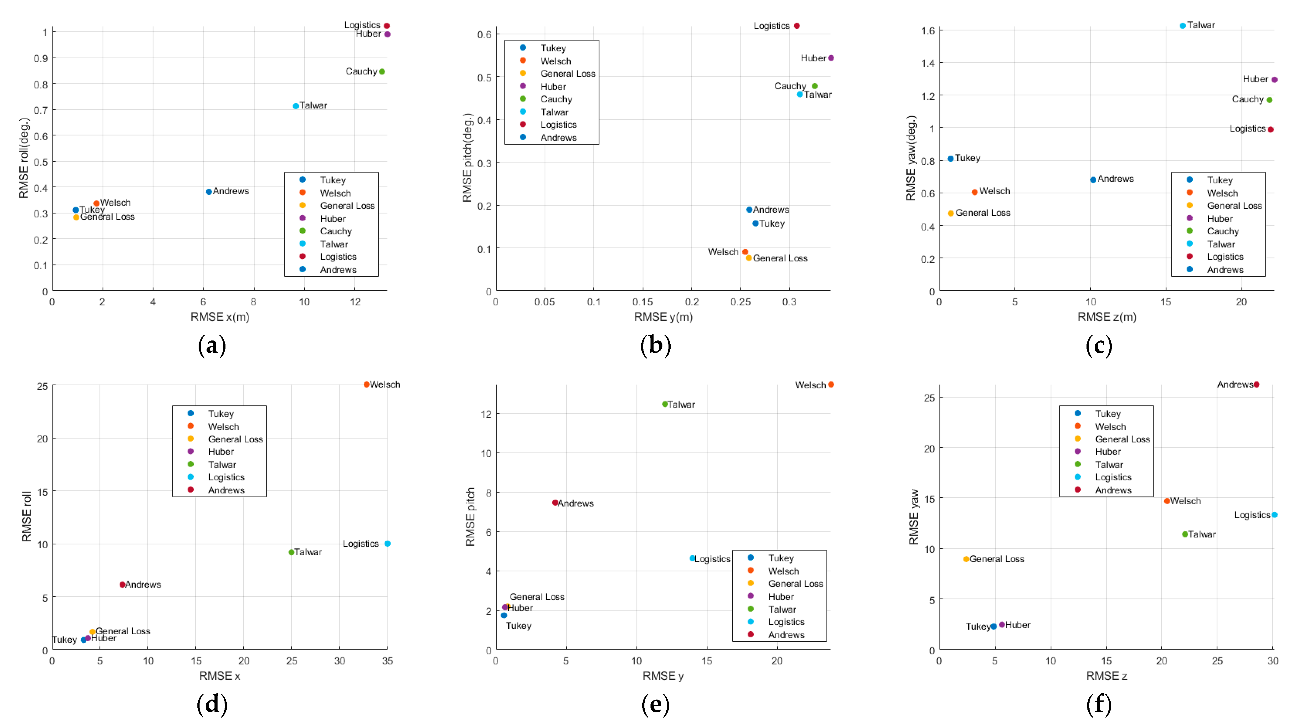
. Figure 8, Figure A1 and Figure A2 illustrate the estimation errors for each axis, plotting the position RMSE along the x-axis and orientation RMSE along the y-axis to visualize the axis-specific estimation performance.

Profile 1 was conducted under conditions in which only the position of the chaser changed. According to the MBT estimation results, the General Loss and Tukey estimators showed superior performance in position and orientation estimation. In terms of the positional accuracy, the General Loss achieved RMSE values of 1.0133 m (x), 0.2606 m (y), and 0.8554 m (z), significantly outperforming Tukey, which yielded 1.2327 m (x) and 1.4434 m (z).

For orientation estimations, General Loss also provided the most accurate results, achieving RMSEs of 0.3197° (roll), 0.1805° (pitch), and 0.6423° (yaw). Regarding the computational efficiency, Huber (22.8028 ms) and Cauchy (23.1106 ms) showed the fastest computation time per frame, whereas General Loss and Tukey required 51.0111 ms and 26.0755 ms, respectively, representing 123.71% and 14.35% increases relative to Huber. In contrast, Welsch (219.9172 ms), Talwar (114.7814 ms), Logistic (143.7517 ms), and Andrews (201.8872 ms) showed relatively high computational costs.

The lowest estimation errors by axis were observed with General Loss (x-axis), General Loss and Welsch (y-axis), and General Loss (z-axis), as shown in Figure 8a–c. Overall, General Loss, Welsch, and Tukey consistently ranked among the top-performing estimators for accuracy across all three axes

Profile 2 followed the same trajectory as profile 1, but the chaser continuously tracked the ISS center, involving positional and rotational motion. Tukey showed the best positional accuracy, with RMSE values of 3.2834 m (x), 0.5772 m (y). General Loss also showed competitive performance, achieving RMSE values of 4.1985 m (x), 0.8343 m (y), and 2.4089 m (z). In the orientation estimation, Tukey showed good overall accuracy, with RMSEs of 0.9264° (roll), 1.7462° (pitch), and 2.3079° (yaw).

When transitioning from profile 1 to 2, the computation time increased for most estimators because of the added complexity of simultaneous positional and rotational variations. The most substantial increase was observed for the Huber estimator, which increased by approximately 118.7% (from 22.8028 ms to 49.8701 ms), followed by the Cauchy estimator with a 104.86% increase (from 23.1106 ms to 47.3436 ms). The Tukey and Welsch estimators exhibited moderate increases of 82.59% and 34.12%, respectively. In contrast, the General Loss function showed a relatively modest increase of only 10.74% (from 51.0111 ms to 56.4875 ms). These results suggest that the General Loss estimator maintains stable computational performance even under profile variations, whereas estimators such as Huber and Cauchy are more sensitive to increased complexity, leading to substantial processing time increases.

Across all three axes, General Loss, Tukey, and Huber consistently ranked among the most precise estimators as shown in Figure 8d–e. These findings align with the profile 1 results (Table 3) confirming the superior performance of General Loss and Tukey in position-dominant and orientation-dominant profiles.

Profile 3 repeated the position-only trajectory of profile 1 with the displacements in the y-z plane reduced to 75% of their original magnitude. According to the MBT estimation results, the General Loss delivered the most accurate solution on all six degrees of freedom, returning RMSE values of 2.909 m (x), 0.3649 m (y), 0.5905 m (z), 0.7289° (roll), 0.4317° (pitch), and 0.9193° (yaw). Tukey consistently produced the next-lowest error RMSE, whereas Welsch and Cauchy registered z-axis position RMSEs exceeding 10 m.

Profile 4 repeated the position-only trajectory of profile 2 with the displacements in the y–z plane reduced to 75% of their original magnitude. In this profile, Huber achieved the best performance on the two translational axes and one rotational axis, with RMSEs of 1.3870 m (x), 0.6188 m (y), and 3.2513° (yaw). General Loss exhibited a yaw RMSE of 11.2655°, representing a 246% increase relative to Huber’s 3.2513°.

Profile 5 repeated the position-only trajectory of profile 1 with the displacements in the y-z plane reduced to 50% of their original magnitude. Under these benign conditions, all estimators except Huber, Cauchy, and Logistic achieved sub-meter and sub-degree accuracy. Talwar and Welsch achieved the lowest errors across the three positional and three rotational axes, with RMSEs of 0.7776 m (x, Talwar), 0.1353 m (y, Welsch), 0.3322 m (z, Talwar), 0.2171° (roll, Welsch), 0.1172° (pitch, Talwar), and 0.4808° (yaw, Welsch). General Loss demonstrated competitive performance across all axes, achieving RMSE values of 0.9703 m (x), 0.1417 m (y), and 0.6347 m (z) in position and 0.2655° (roll), 0.1550° (pitch), and 0.7000° (yaw) in orientation. Although Talwar and Welsch provided the lowest errors on specific axes, the differences over General Loss remained within a narrow margin of less than 10%, indicating that General Loss maintains robust estimation accuracy under these favorable conditions while ensuring consistent performance across all degrees of freedom.

Profile 6 repeated the position-only trajectory of profile 2 with the displacements in the y-z plane reduced to 50% of their original magnitude. Cauchy failed to achieve model alignment and produced no valid estimate. General Loss showed the greatest overall accuracy, achieving RMSEs of 5.2132 m (x), 0.4000 m (y), 1.5183° (roll), and 3.4539° (yaw). Tukey provided the best z-axis position accuracy at 5.2951 m, while Logistic achieved the lowest RMSE on the pitch axis at 1.2972°. In contrast, Welsch and Logistic once more displayed z-axis errors exceeding 20 m.

4. Discussion

In the discussion, we interpret the profile-wise Errors of General Loss and the seven M-estimators, focusing on profiles 2, 4, and 5. First, in profile 2, Tukey showed the best positional accuracy, with RMSE values of 3.2834 m (x) and 0.5772 m (y). General Loss also showed competitive performance, achieving RMSE values of 4.1985 m (x), 0.8343 m (y), and 2.4089 m (z). In the orientation estimation, Tukey showed good overall accuracy, with RMSEs of 0.9264° (roll), 1.7462° (pitch), and 2.3079° (yaw). 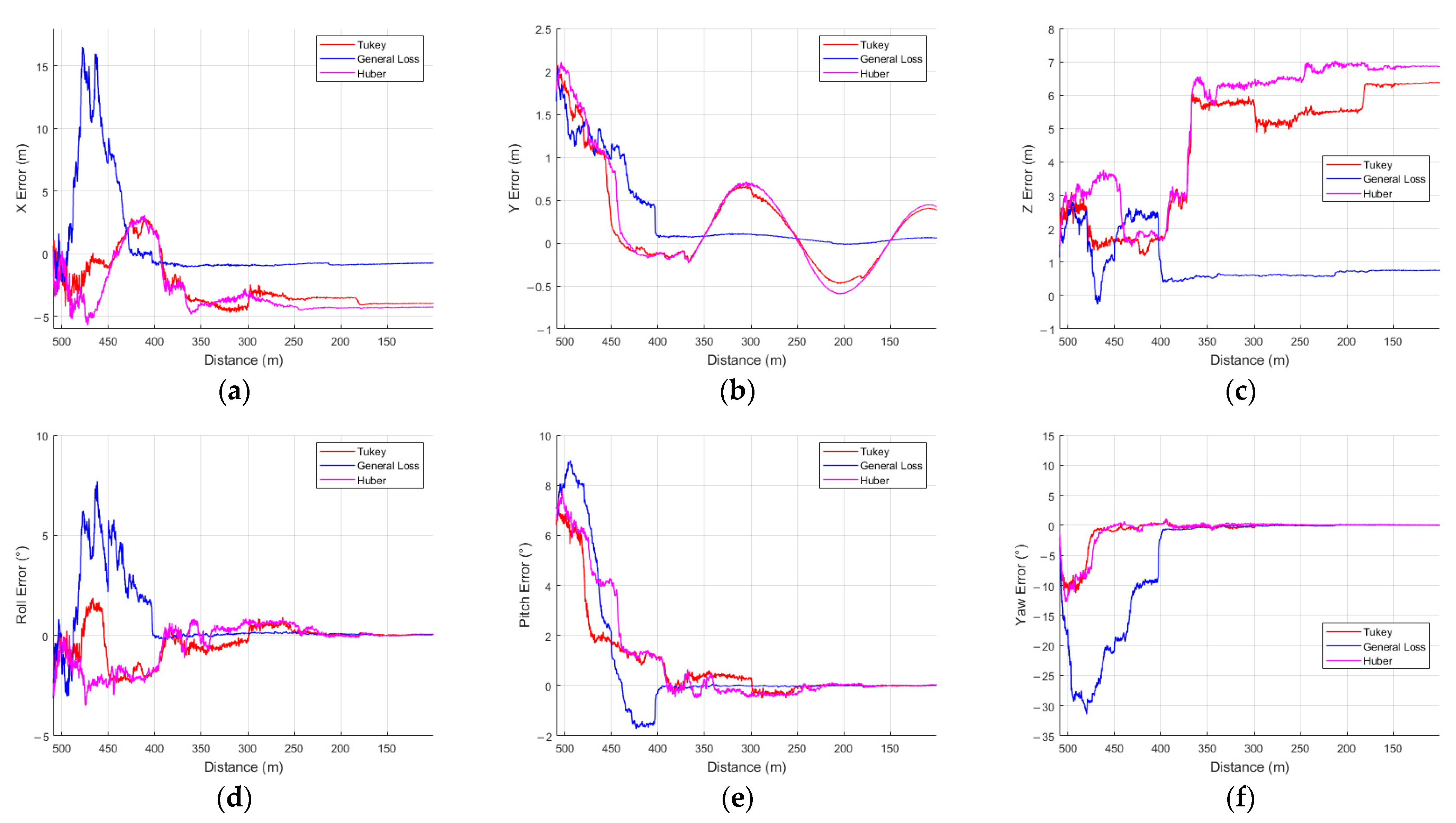Figure 9a–f shows the error plots with relative distance on the x-axis, comparing three M-estimators (Tukey, General Loss, and Huber) in profile 2.

As Figure 9a–f illustrates, the General Loss estimator completed model alignment more slowly than Tukey and Huber on every axis except z. However, in Figure 9c,f, Tukey and Huber each exhibit gross misalignments of approximately 5 m and 6 m, respectively, because the tracker converges exclusively on the left and right edges of the panel, while completely misaligning the top and bottom edges. Consequently, by the end of the simulation, General Loss is the only one of the three estimators that maintains a globally consistent geometric fit, as shown in Table A1.

Moreover, because the tracker fails to capture the panel’s top and bottom edges, the virtual contour remains locked onto the lateral edges and oscillates along the z-axis, producing a back-and-forth motion that manifests as a sinusoidal signature in the y-axis error.

Despite these tracking slips, the Tukey and Huber estimators still converge and maintain low attitude errors. Even when the central panel is missed, the algorithm stabilizes on the symmetric left- and right-hand faces of the solar-array frame, which provide enough geometric cues to anchor the pose solution.

The larger RMSE of the General Loss estimator on the x and yaw axes stems from a substantial spike in error during the initial pose alignment process. In IRLS, numerical divergence becomes more probable as the Jacobian ($J^{T}WJ$) matrix grows ill-conditioned [20], and this condition number is strongly linked to the weight entropy [21]. Within the IRLS framework, weight entropy quantifies how evenly the sample weights are distributed. High entropy—i.e., more evenly distributed weights—generally enhances numerical stability and promotes robust convergence. Conversely, low entropy implies that only a few samples carry most of the weight, increasing the risk of instability.

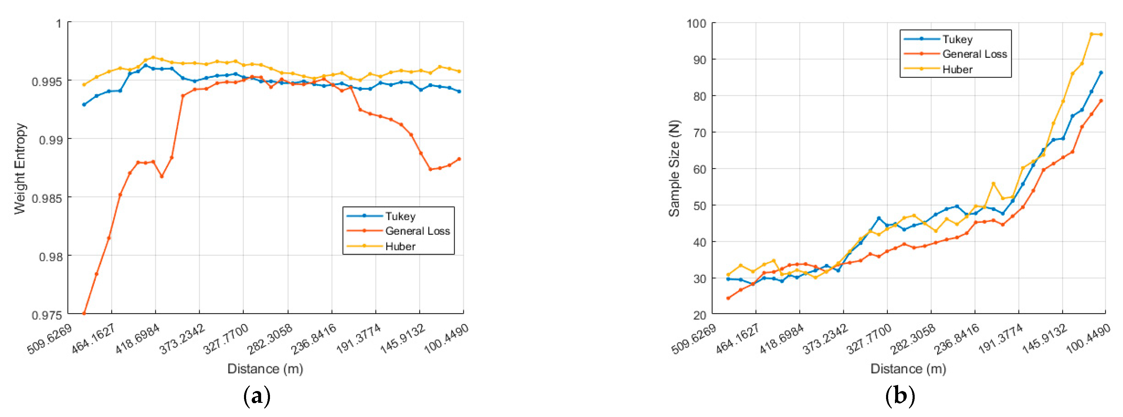
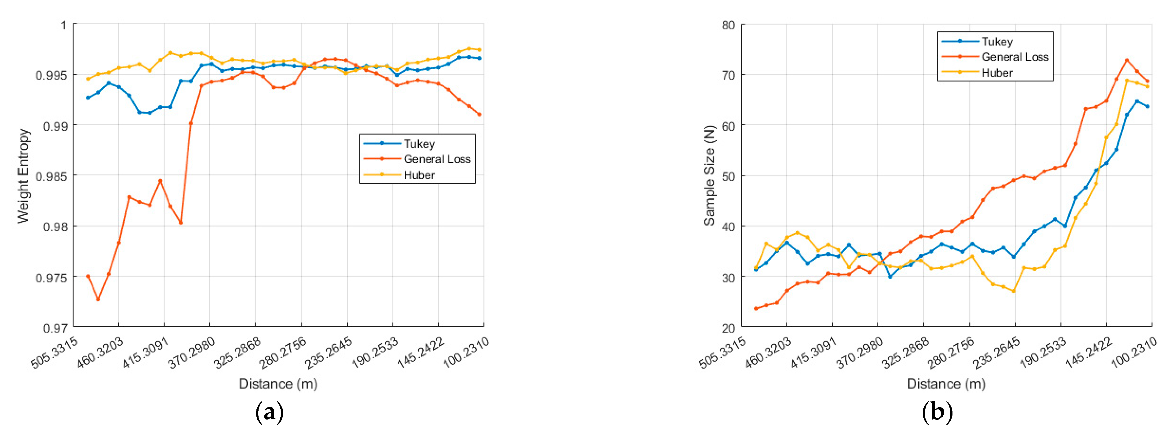
For the ISS MBT experiments, we computed the weight-entropy of the last IRLS iteration at every frame, divided the chaser–ISS separation into 10 m bins, and averaged the weight-entropy within each bin. The resulting profile is plotted in Figure 7, and weight-entropy is defined in Equation (26).

$$H_{avg}\left(\mathsf{\omega }\right)={\displaystyle \frac{-\sum _{i=1}^N{\mathsf{\omega }}_i\log {\mathsf{\omega }}_i}{\sqrt{N}}}$$

(26)

where ${\omega }_i$ denotes the weight assigned to the $i_{th}$ correspondence, obtained from the normalized residual ${\omega }_i={\displaystyle \frac{\psi \left(u_i\right)}{u_i}}$, and N denotes the number of sample points.

In the numerical results, General Loss starts with a markedly lower weight-entropy than Tukey and Huber. From the first 10 m bin, its entropy increases steadily and reaches a level comparable to Tukey and Huber at about 400 m. This rise in entropy—i.e., more uniformly distributed weights, which enhances numerical stability and supports robust convergence—drives a sharp reduction in six-degree-of-freedom pose estimation errors, culminating in successful model tracking (Figure 10).

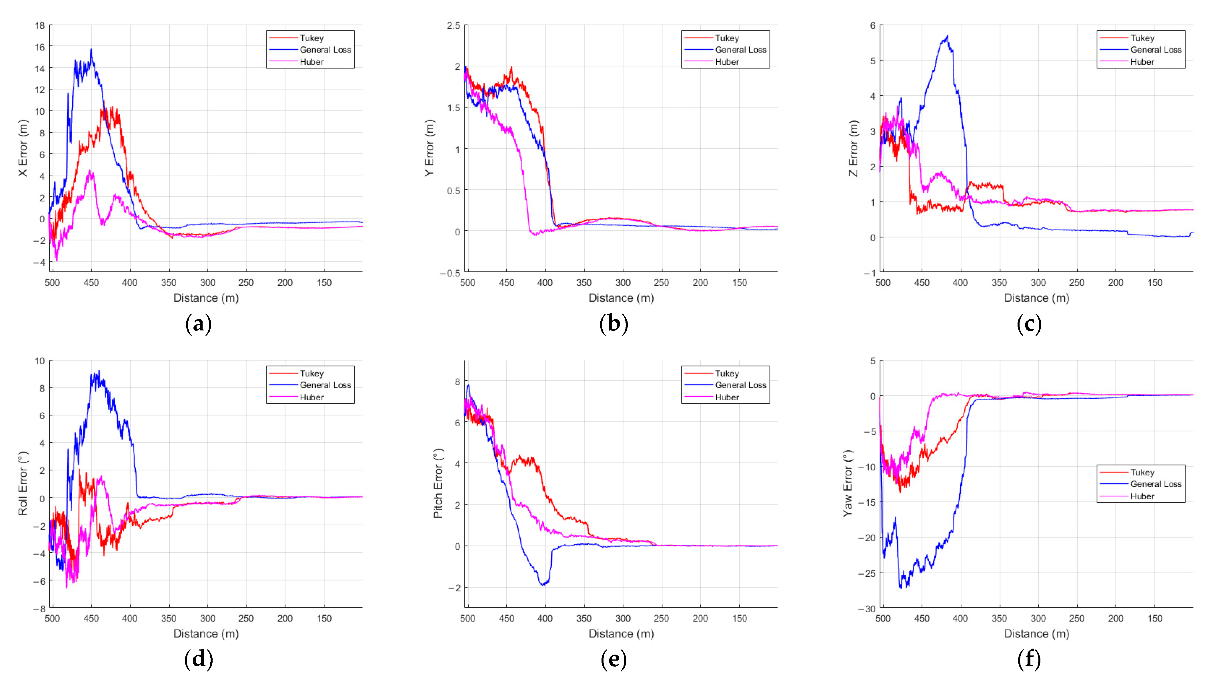
In profile 4, Huber achieved the best performance on the x, y, and yaw axes, with RMSE values of 1.3870 m (x), 0.6188 m (y), and 3.2513° (yaw), respectively. Tukey showed the lowest errors on the z and roll axes, while General Loss achieved the lowest RMSE on the pitch axis. Figure 11a–f shows the results comparing three M-estimators (Tukey, General Loss, and Huber) in profile 4. As shown in Figure 11a–f, unlike in profile 2, all three estimators successfully tracked the model throughout the profile. For General Loss, however, large transient errors occurred during model alignment on every axis except for the y and pitch axes.

Following the previous analysis, Figure 12 shows the weight entropy H as a function of the relative distance. At 500 m, General Loss starts approximately 0.02 lower than Tukey and Huber; it then climbs sharply around 485 m, and by 390 m, all three estimators exhibit nearly identical entropy levels. This behavior corresponds to the divergence observed in the x, z, roll, and yaw axes and the model alignment that occurs near 400 m.

In profile 5, all estimators achieved sub-meter and sub-degree accuracy. Talwar yielded the minimum RMSE on every axis (0.777 m, 0.143 m, and 0.333 m for x, y, and z, respectively, and 0.266°, 0.117°, and 0.701° for roll, pitch, and yaw, respectively)

However, Welsch, Talwar, Logistic, and Andrews estimators exhibited larger position and orientation errors in other profiles. As observed in the tracking results, these three M-estimators, including Welsch, showed significantly higher RMSE values, likely due to incorrect tracking caused by the MBT algorithm occasionally locking onto an unintended ISS solar panel, as shown in Figure 13a,b. Consequently, the superior accuracy observed for all estimators, particularly for Talwar and Welsch, should be interpreted as a result specific to profile 5 and cannot be generalized to the other profiles.

5. Conclusions

A vision-based MBT approach was used to achieve the high-precision relative navigation required for OOS missions. Specifically, the General Loss function within the MBT framework and its performance was evaluated and compared with seven other robust M-estimators: Tukey, Welsch, Huber, Cauchy, Talwar, Logistic, and Andrews. Simulations were conducted in a ROS–Gazebo environment, emulating a rendezvous profile with the ISS. Six distinct approach profiles, involving different chaser orientations and initial radial offsets (100%, 75%, and 50%), were designed to assess estimator performance under various ISS proximity tracking scenarios. The performance of each estimator was assessed using the RMSE for position (x, y, z) and orientation (roll, pitch, yaw).

Among all M-estimators, General Loss was the only estimator that successfully achieved complete pose alignment across all profiles. In profiles 1, 3, and 6, it provided high accuracy throughout the entire simulation and at the end point (at 100 m relative distance in x-axis), while maintaining stable computational efficiency. In profiles 2, 4, and 5, General Loss exhibited higher RMSE values over some segments compared to other estimators; however, these errors were attributed to the initial offsets applied to the initial poses estimated using SPNv2, which led to transient errors during the pose alignment process. By the end of the simulation, these errors were reduced to the sub-meter and sub-degree levels. The adaptive capability of General Loss to dynamically adjust the loss function shape based on the residual distribution enabled robust performance under various noise conditions and in the presence of outliers. In contrast, the Huber and Cauchy estimators were more sensitive to extreme outliers, resulting in higher estimation errors, while the Welsch and Logistic estimators required longer computational times and showed larger errors. Future research will aim to extend the application of the General Loss-based MBT approach to more challenging conditions, including variable lighting environments, non-standard object geometries, and multi-sensor fusion profiles, with the goal of advancing high-precision and highly reliable relative navigation technologies for real-world OOS missions.