Article

Research on Parameter Prediction Model of S-Shaped Inlet Based on FCM-NDAPSO-RBF Neural Network

College of Energy and Power Engineering, Nanjing University of Aeronautics and Astronautics, Nanjing 210016, China
*
Author to whom correspondence should be addressed.
Aerospace 2025, 12(8), 748; https://doi.org/10.3390/aerospace12080748
Submission received: 14 May 2025 / Revised: 18 July 2025 / Accepted: 11 August 2025 / Published: 21 August 2025
(This article belongs to the Section Aeronautics)

Abstract

To address the inefficiencies of traditional numerical simulations and the high cost of experimental validation in the aerodynamic–stealth integrated design of S-shaped inlets for aero-engines, this study proposes a novel parameter prediction model based on a fuzzy C-means (FCM) clustering and nonlinear dynamic adaptive particle swarm optimization-enhanced radial basis function neural network (NDAPSO-RBFNN). The FCM algorithm is applied to reduce the feature dimensionality of aerodynamic parameters and determine the optimal hidden layer structure of the RBF network using clustering validity indices. Meanwhile, the NDAPSO algorithm introduces a three-stage adaptive inertia weight mechanism to balance global exploration and local exploitation effectively. Simulation results demonstrate that the proposed model significantly improves training efficiency and generalization capability. Specifically, the model achieves a root mean square error (RMSE) of 3.81 × 10 8 on the training set and 8.26 × 10 8 on the test set, demonstrating robust predictive accuracy. Furthermore, 98.3 % of the predicted values fall within the y = x ± 3 β confidence interval ( β = 1.2 × 10 7 ). Compared with traditional PSO-RBF models, the number of iterations of NDAPSO-RBF network is lower, the single prediction time of NDAPSO-RBF network is shorter, and the number of calls to the standard deviation of the NDAPSO-RBF network is lower. These results indicate that the proposed model not only provides a reliable and efficient surrogate modeling method for complex inlet flow fields but also offers a promising approach for real-time multi-objective aerodynamic–stealth optimization in aerospace applications.

1. Introduction

The total pressure recovery coefficient of the aero-engine inlet is the core index to evaluate its aerodynamic performance, which directly affects the thrust efficiency and fuel economy of the engine. For the design of S-shaped inlet in stealth aircraft, how to maintain high total pressure recovery coefficient and low distortion index while realizing radar wave scattering suppression is the key challenge of current aerodynamic–stealth collaborative optimization [1,2]. The traditional CFD numerical simulation method based on Reynolds-averaged Navier–Stokes equations (RANS) [3,4,5] can provide high-precision prediction, but its huge computational cost seriously limits the efficiency of design iteration. However, the experimental test [6] is limited by the size effect generated by the wind tunnel design and the difficulty of covering the setting of all working conditions, which makes it difficult to meet the current rapid iterative development requirements of the aircraft.
In order to solve the above problems, data-driven models based on machine learning algorithms have become a research hotspot. Wang et al. [7] used generalized regression neural network, radial basis function (RBF) neural network, support vector regression and random forest to develop and establish a data-driven aeroengine exhaust gas temperature baseline prediction framework based on machine learning algorithm. Liu et al. [8] combined the RBF with the data-driven pre-screening optimization algorithm to establish a fast aerodynamic optimization platform for axial flow compressors. Zhang et al. [9] proposed an adaptive model predictive control (AMPC) based on RBF model for trajectory tracking. In further research, the combination of intelligent algorithms is becoming the key to the performance breakthrough of such models. For example, Wei et al. [10] found in the prediction of compressor characteristics that the DPSO-RBFNN model significantly improved the accuracy and efficiency of the HCF life probability analysis of compressor blades through the deep integration of intelligent optimization algorithms and engineering analysis. Wu et al. [11] coupled the improved MOPSO algorithm with the DBN surrogate model to perform multi-objective aerodynamic optimization on the constrained rotor airfoil, and the aerodynamic performance was significantly improved. Although the classical particle swarm optimization (PSO) algorithm is used for parameter tuning, its linearly decreasing inertia weight strategy easily leads to premature convergence [12]. On the other hand, the nonlinear characteristics of the inlet flow need to intelligently reduce the dimension of the input data, but the existing research still relies on the empirical threshold for the determination of the optimal clustering number. Simple direct classification lacks dynamic adaptability and needs to be processed by fuzzy rules. For example, refs. [13,14] established an aircraft engine model based on T-S fuzzy.
In this paper, a nonlinear dynamic adaptive PSO (NDAPSO) prediction model combining FCM and RBF neural network is proposed. The second chapter introduces the relevant theoretical basis; the third chapter analyzes the dynamic nonlinear adaptive strategy design process of NDAPSO algorithm in detail; in the fourth chapter, the feature distribution of experimental data is optimized by FCM to verify the generalization ability of the total pressure recovery coefficient prediction model. The fifth chapter summarizes the research results and puts forward the future direction.

2. Structural Coupling Design of S-Shaped Inlet Considering Stealth Performance

2.1. The Total Pressure Recovery Coefficient of Inlet

The inlet is a kind of gas collecting device. Its main function is to supply a certain flow rate, pressure and flow rate of air to the engine by means of rectification, deceleration and pressurization under the condition of minimizing the loss of air flow. The inlet must meet the strict requirements of the engine on the target parameters while ensuring good aerodynamic performance, so as to ensure that the engine can operate continuously, stably and efficiently under given conditions.
σ = P 1 * P 0 *
Among them, P 1 * is the total pressure of the outlet airflow of the inlet, and P 0 * is the total pressure of the free unperturbed airflow. The total pressure recovery coefficient σ represents the flow loss of the airflow through the inlet. In general, the larger the value, the smaller the thrust loss, which can better overcome the flow resistance. Figure 1 is the overall structure of the S-shaped inlet used in this paper. The total pressure recovery coefficient of a subsonic inlet in flight is generally σ 0.94 , 0.98 . The total pressure recovery coefficient σ , as a key index to evaluate the aerodynamic performance of the S-shaped inlet, directly reflects the energy loss of the air flow through the inlet. In the S-shaped inlet structure, due to its double-bending geometric characteristics, the airflow will produce a series of complex three-dimensional flow phenomena inside, including boundary layer separation, backflow, secondary flow induced vortex, etc. These phenomena will significantly destroy the uniformity and stability of the airflow, resulting in increased total pressure loss. When the incoming mach number increases or the angle of attack changes greatly, the pressure gradient in the curved region increases, which is easy to cause local flow separation, while the large offset or unreasonable diffuser structure will strengthen the curved induced vortex, resulting in a significant distribution difference in the total pressure at the outlet surface and a decrease in the σ value. It can be said that σ is not only a characterization of the overall intake effect, but its change essentially reflects the comprehensive influence of the unsteady flow behavior inside the S-shaped inlet. Therefore, in this study, taking σ as the output index not only has important engineering significance, but also fully reflects the learning ability of the model to complex flow characteristics.
D ¯ = P 1 * max P 1 * min P ¯ 1 *
In the formula, P 1 * max represents the maximum value of the total pressure of the air flow at the outlet section of the inlet, P 1 * min represents the minimum value of the total pressure of the air flow at the outlet section of the inlet, and P ¯ 1 * represents the average total pressure of the total area of the inlet outlet. The larger the distortion coefficient D ¯ , the more unstable the airflow, which should be avoided.
Q = ρ V A
Among them, Q is the air quality flow, ρ is the fluid density, A is the size of the corresponding cross-sectional area, and V is the average atmospheric velocity passing through the cross-section. If the flow is large enough, the engine can use enough atmosphere to generate thrust. Figure 1 is the overall structure of the S-shaped inlet used in this paper.
According to the above analysis, it can be seen that the aerodynamic parameters related to the inlet have a strong correlation. However, in practice, it is often necessary to meet the ideal values of multiple aerodynamic parameters and consider leaving enough safety margin. Therefore, considering the actual needs of the project, set such target parameters:
σ 0.96 D ¯ 0.8 Q 1.25 kg / s

2.2. The S-Shaped Inlet

Relevant research shows that within the range of 30 in front of the fighter, the inlet inlet accounts for about 40 % of the radar wave intensity scattering source [15,16,17]. Therefore, it is necessary for the design of the inlet to have a certain stealth performance. As shown in Figure 2, in the structure of the inlet, compared with the traditional inlet shape, the inlet is designed to be semi-circular. This is because the semi-circular inlet does not easily produce strong specular reflection, but rather more edge diffraction than specular scattering, which can achieve a better stealth effect. At the same time, the semi-circular inlet can better adapt to different flight angles of attack, making the air flow more uniform and stable when entering the inlet.
The diffuser design of the S-shaped inlet is the core part to ensure the effective operation of the inlet. The S-shaped inlet studied in this paper adopts a design method of S-shaped inlet with large offset and short diffuser [18]. Among them, the change law of the center line and the change of the cross-sectional area are particularly important. Combined with a large number of experimental and numerical simulation results of the aerodynamic characteristics of the S-shaped inlet in References [19,20,21], it is shown that the design of the S-shaped inlet adopts the center line of the front and slow and the cross-sectional area change law of the slow and slow, which can obtain good aerodynamic and stealth performance at the same time. When guiding the airflow through the complex curved section, it performs rectification and pressurization to ensure uniform and stable airflow and provide good intake conditions for the compressor. At the same time, the design of the multiple bending section can reflect and attenuate the radar wave, and reduce the radar scattering cross-section so that the radar wave cannot be directly irradiated to the front end of the engine compressor with a certain stealth performance. Figure 3 shows the diffuser section of the S-shaped inlet and its centerline structure curve.
The change rule of the center line is Equation (5), where y h is the longitudinal coordinate of center line of the diffuser, H is the longitudinal offset of the diffuser, and x h is transverse coordinate of the diffuser centerline; L d i f f is the length of the diffuser. In the first half of the diffuser section, the centerline changes rapidly, so as to quickly adjust the flow direction; in the latter part, the change of the centerline gradually slows down, so that the airflow smoothly transitions before entering the downstream. This design achieves a good balance between total pressure recovery and distortion control.
y h = H [ 3 ( x h L d i f f ) 4 8 ( x h L d i f f ) 3 + 6 ( x h L d i f f ) 2 ]
The change rule of the cross-sectional area is Equation (6), where A 1 is the inlet area of the diffuser; A 2 is the outlet area of the diffuser. The area change rate of the cross-section of the diffuser section along the axial direction remains uniform, and the pressure gradient is relatively stable, which avoids the phenomenon of airflow separation to a certain extent and improves the total pressure recovery coefficient.
A A 1 = ( A 2 A 1 1 ) [ 2 ( x h L d i f f ) 3 + 3 ( x h L d i f f ) 2 ] + 1
As shown in Figure 4, the outlet contraction section presents a cylindrical ring structure, and the middle part accommodates a motor structure similar to a cylinder, which plays a role similar to a rectifier cone, guiding the airflow along the common axis direction in the annular channel of the structure. The outlet compression section increases the airflow velocity by gradually reducing the cross-sectional area of the airflow channel. At the same time, part of the kinetic energy is converted into pressure energy, and the airflow entering the engine compressor structure has a higher total pressure.

3. Nonlinear Dynamic Adaptive Particle Swarm Optimization Algorithm

3.1. Standard Particle Swarm Optimization

PSO is an intelligent optimization algorithm for finding the optimal solution of the objective function by simulating the cooperation and competition of particle swarm in the search space. Because of its simple implementation and high computational efficiency, it is widely used in function optimization, neural network training, pattern recognition and other fields. In the PSO algorithm, the particle swarm is composed of several particles, each particle representing a candidate solution in the solution space of the problem. The position and velocity of the particle determine the change in state. Each particle continuously updates its position and velocity by following the individual optimal solution ( p b e s t ) and the global optimal solution ( g b e s t ).
v i k + 1 = ω v i k + c 1 r 1 ( p b e s t i k p i k ) + c 2 r 2 ( g b e s t i k p i k )
p i k + 1 = p i k + v i k + 1
Here, v i k denotes the velocity of the particle i at the iteration k; p i k represents the position of the particle i at the iteration k; w represents the inertia weight; c 1 , c 2 represent the learning factor; r 1 , r 2 show random numbers; p b e s t i k denotes the individual optimal position of the particle i; g b e s t i k denotes the global optimal position. The inertia weight w controls the influence of particle velocity on the subsequent motion. The optimal inertia weight needs to be selected as appropriate to balance the global search and local development capabilities.

3.2. Improved Particle Swarm Optimization

The traditional PSO optimization uses the linear decreasing weight strategy to dynamically adjust the inertia factor, so as to achieve rapid optimization. However, in the actual optimization process, the inertia weight is uniformly attenuated, lacking the ability to respond to the dynamic state of the optimization process, and it is easy to fall into major defects such as local optimum and slow convergence speed.
ω ( t ) = ω max T max t T max + ω min t T max
Among them, ω max and ω min are the maximum and minimum inertia weights, respectively; t is the current number of iterations, and T max is the maximum number of iterations.
Aiming at the design of inertia weight, this paper combines a new PSO particle population evolutionary adaptation index function k ( t ) , with the nonlinear feature mapping activation function S ( x ) in RBF neural network, and proposes a PSO optimization control strategy based on nonlinear adaptive dynamic inertia weight to adapt to the global search and local development ability of the algorithm.

3.3. Dynamic Fitness Standard Deviation Based on Population Convergence State

The population evolution fitness index function k ( t ) is used to evaluate the diversity of the current population and determine the change range of the inertia weight.
k ( t ) = 1 , t = 1 StdFit ( t ) StdFit ( t 1 ) , t > 1
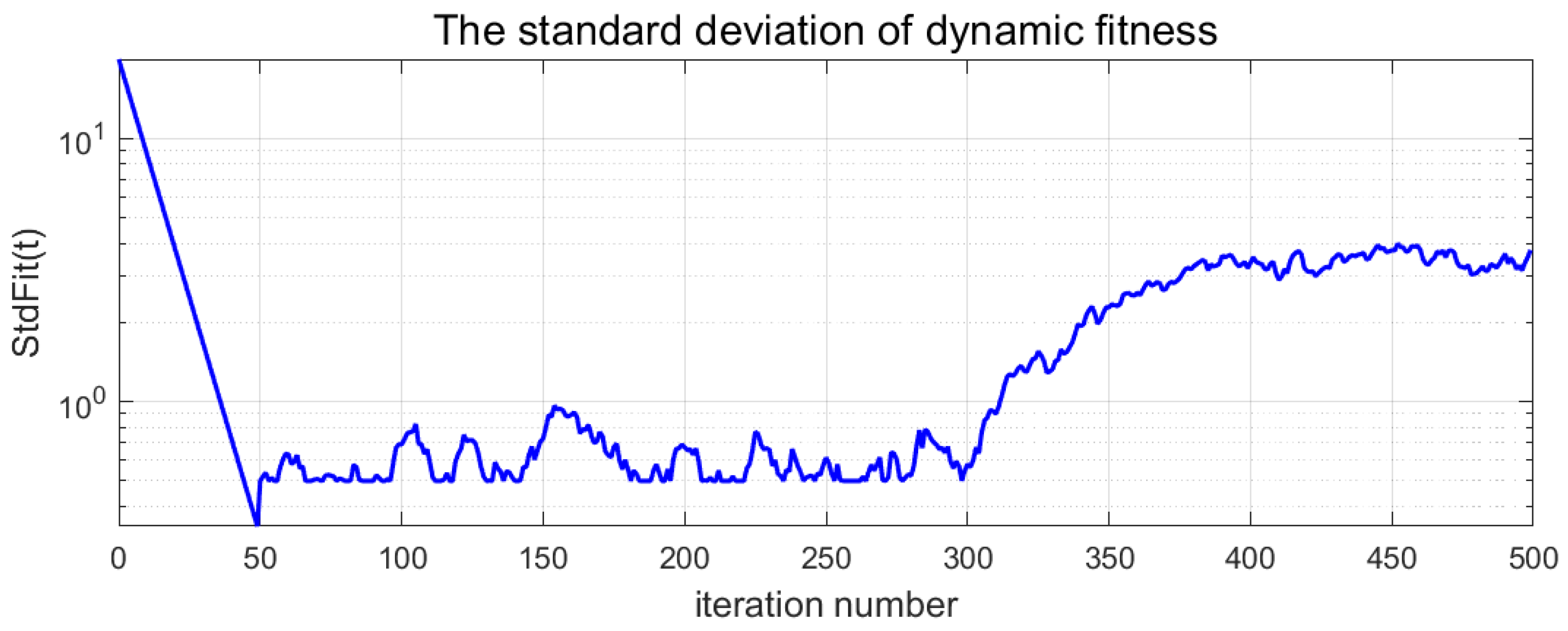
StdFit ( t ) represents the standard deviation of the fitness of the current population particles, which is used to capture the convergence dynamics of the population. When k ( t ) increases, it represents the population divergence (exploration enhancement); when k ( t ) decreases, it indicates population convergence (development enhancement).
StdFit ( t ) = 0.92 StdFit ( t 1 ) , 0 t 0.3 T max 0.98 StdFit ( t 1 ) + 0.05 N 0 , 0 . 05 2 , 0.3 T max < t 0.7 T max StdFit ( t 1 ) ( 1 + 0.04 N ( 0 , 1 ) ) + 0.1 M ( 0 , 1 ) , 0.7 T max < t T max
Figure 5 shows the three-stage attenuation characteristics of the fitness standard deviation ( StdFit ( t ) ): the early stage corresponds to the exponential decay period ( 0 t 0.3 T max ), StdFit ( t ) decays exponentially from the initial value of 20 to 3.17 ± 0.45 , and the particle population quickly gathers to the global optimal region. In the middle stage, it belongs to the stationary convergence period ( 0.3 T max < t 0.7 T max ). The random disturbance term is introduced, and the attenuation rate is reduced to 2. The goodness of fit between the particle position distribution and the normal distribution in this stage is D = 0.0078 , which indicates that the algorithm maintains reasonable diversity. The later stage is the sensitive fluctuation period ( 0.7 T max < t T max ), and the random disturbance term is further introduced. The relative fluctuation range is 4 % , and the success probability of the algorithm to escape from the local optimal solution is further improved.

3.4. Dynamic Adaptation Factor Based on Inertia Weight Change

The S ( x ) function (Equation (12)) has a good balance between linearity and nonlinearity. The inertia weight w ( t ) (Equation (14)) is mapped by the S ( x ) function, and an adaptation factor b is added. In this way, a PSO optimization algorithm based on nonlinear dynamic adaptive inertia weight is designed.
S ( x ) = exp ( x ) 1 + exp ( x )
z = 10 b ( 2 t k ( t ) T max 1 )
ω ( t ) = ω max 1 + e z + ω min · e z 1 + e z
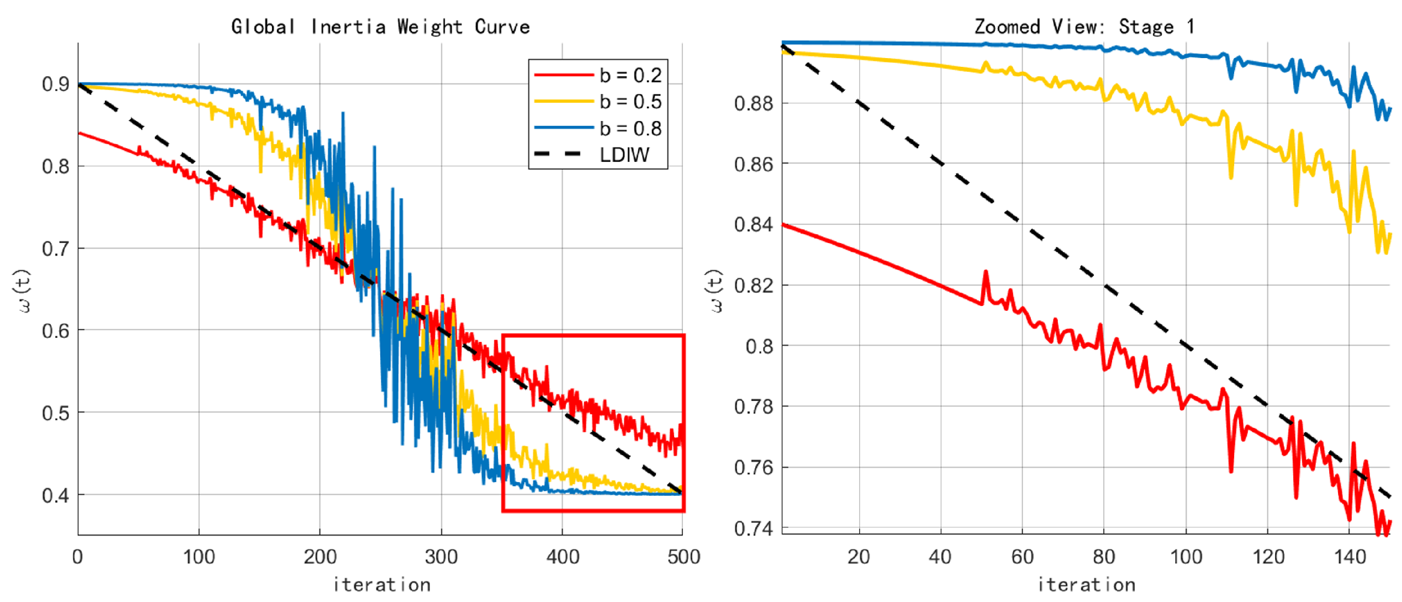
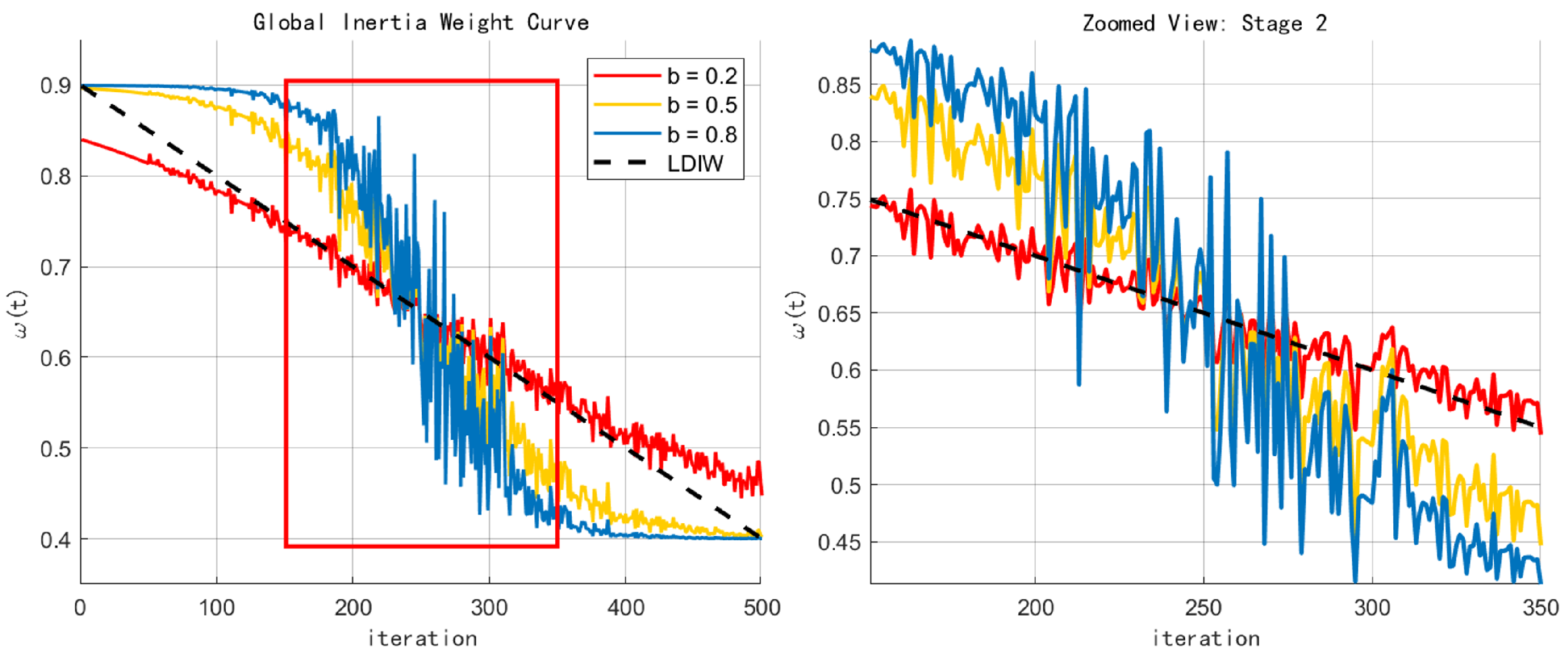
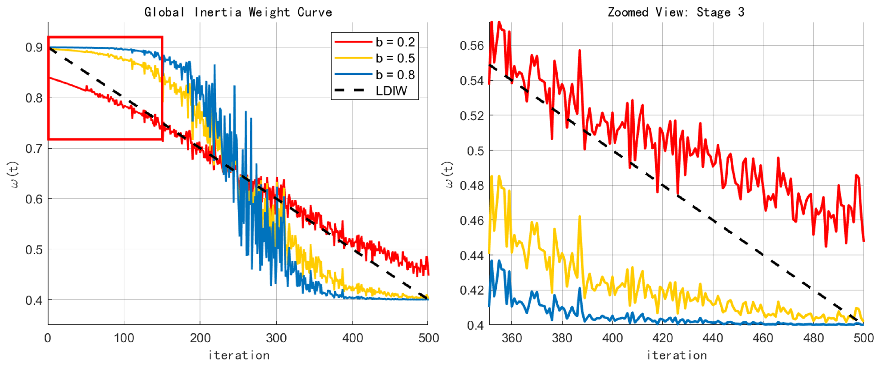
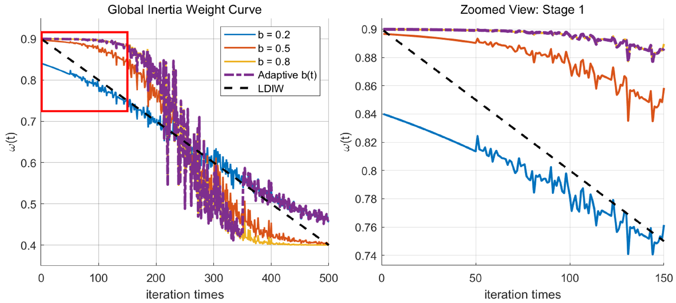
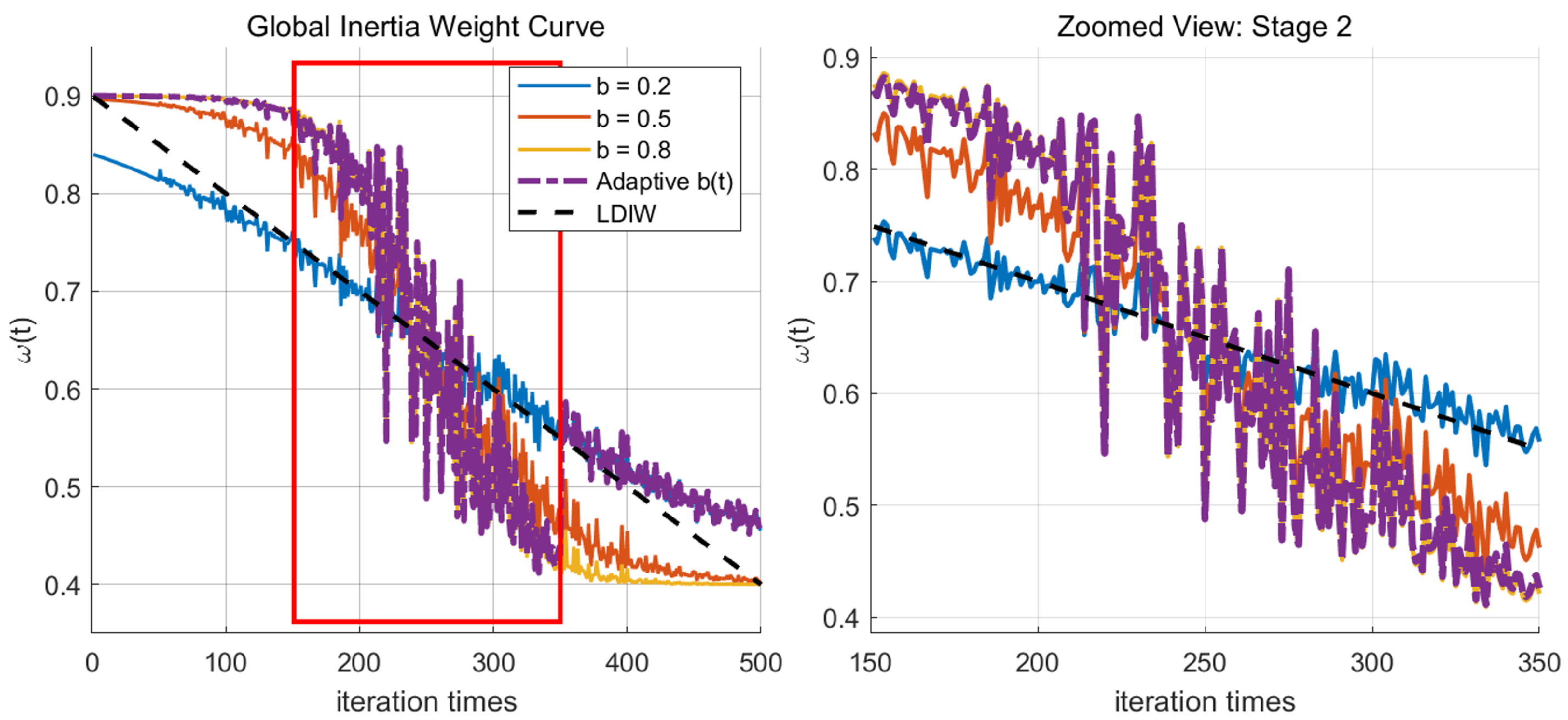
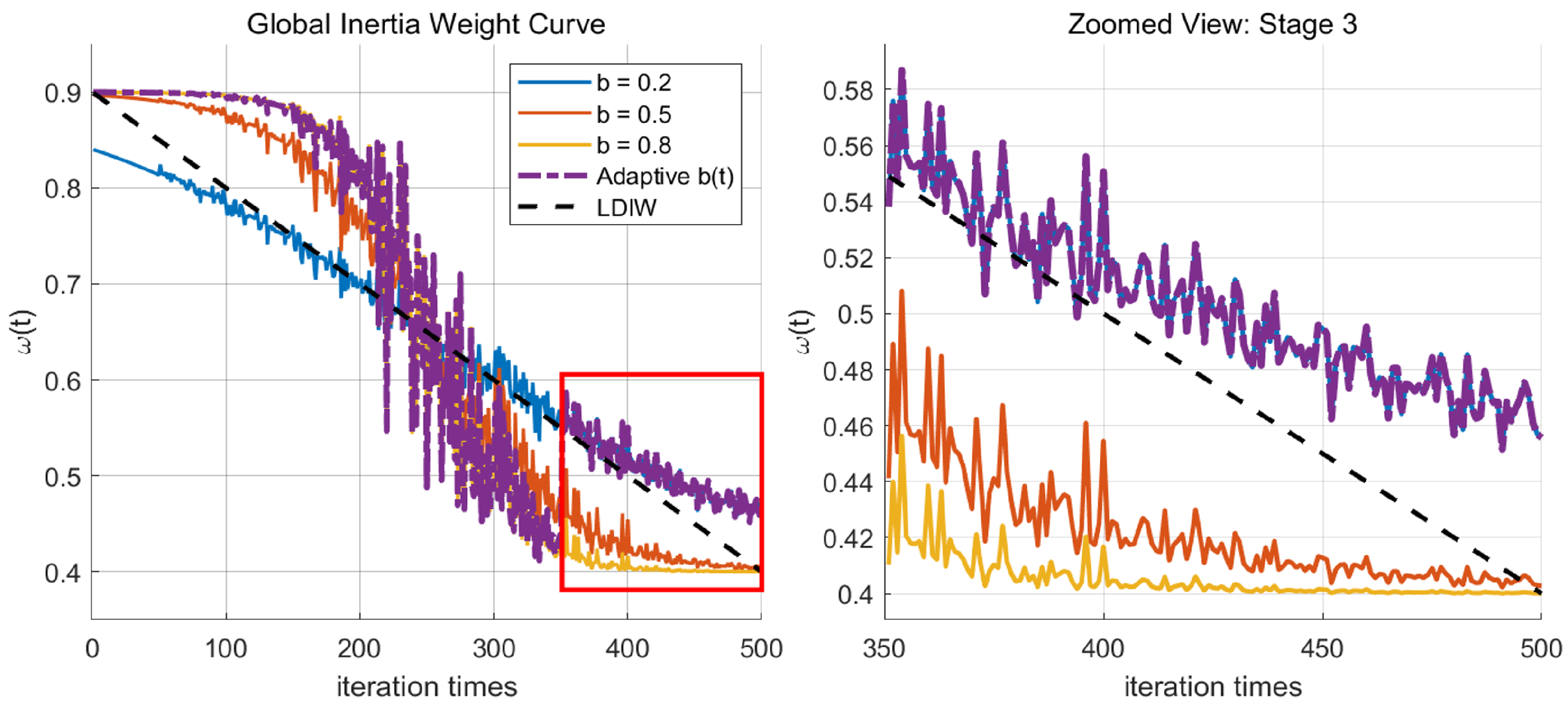
Figure 6, Figure 7 and Figure 8 show the inertia weight w ( t ) adaptive evolution curve of the nonlinear adaptive control strategy and the traditional linear decreasing control strategy (LDIW) under different adaptation factors b in the three stages of the PSO algorithm. The left side of each image is the whole curve, and the right side is the corresponding stage frame area expansion curve. The curve can be divided into three key characteristic stages: In the initial global exploration stage ( 0 t 0.3 T max ), b = 0.8 has a higher inertia weight, and the use of a higher b design is conducive to strengthening the global exploration ability of the particle swarm in the initial stage. In the medium-term transition phase ( 0.3 T max < t 0.7 T max ), the NDAPSO curve fluctuates significantly (amplitude Δ w max 0.07 ). It can be seen that b = 0.2 is generally close to LDIW, b = 0.5 is close to b = 0.8 , but the curve between the two control groups is quite different. Therefore, the adaptation factor b here needs to be further improved to balance the relationship between exploration and development. In the late local development stage ( 0.7 T max < t T max ), the inertia weight of NDAPSO shows significant local oscillation characteristics. This is because in a series of periodic oscillations, the sudden increase of inertia weight will reset the particle velocity, break away from the local attraction domain and avoid local optimization. Therefore, a lower b = 0.2 design is adopted, which can retain the oscillation to a greater extent than LDIW, enhance the local escape ability in the later stage, and avoid falling into the suboptimal solution.
Combining the optimal parameters of each stage, in order to further dynamically adjust, b is now dynamically designed for a three-stage collaborative mechanism, breaking through the traditional fixed parameter mode, and designing a global adaptive strategy.
b ( t ) = 0.8 0 t 0.3 T max 0.5 + 0.3 sin π t T max 0.3 T max < t 0.7 T max 0.2 0.7 T max < t T max
Figure 9, Figure 10 and Figure 11 show the adaptive evolution curves of the nonlinear global adaptive control strategy, the traditional linear decreasing control strategy (LDIW) and the inertia weight w ( t ) under different adaptive factors b in the three stages of the NDAPSO algorithm. The left side of each image is the whole curve, and the right side is the corresponding stage frame area expansion curve.
According to Equation (15), combined with the analysis of the above chapters, in the early iteration of the PSO algorithm, the attenuation rate and initial value of inertia weight w ( t ) directly affect the global search ability. It can be seen from Table 1 that the diffusion radius R = 5.21 corresponding to b = 0.8 is the largest. In the initial stage, k ( t ) 1 , the inertia weight attenuation rate w t 1 1 + e z ( t ) , b = 0.8 can significantly reduce the attenuation rate compared with other methods, and the average moving speed of particles is 18.7 % higher than that of LDIW. Therefore, the higher adaptive parameter b = 0.8 is adopted to maintain the higher exploration speed of the particles by slowing down the weight attenuation, so as to fully cover the search space, avoid premature local convergence, and provide better initial population distribution for local development in the subsequent stage.
In the middle of the iteration of the PSO algorithm, the sinusoidal period adjustment term is introduced. At this time, b ( t ) 0.2 , 0.8 , amplitude is 0.3, and fundamental frequency is 1 T max . The population state is responded in real time through the sinusoidal term, and the amplitude ensures that the parameter is adjusted within the effective interval. The fluctuation frequency is synchronized with the iteration period to avoid the convergence stability of high-frequency oscillation interference. Through formula coupling, the closed-loop adjustment of b ( t ) w ( t ) k ( t ) b ( t ) is realized, and the dynamic response ability of the algorithm is given. As shown in Table 2, periodic adjustment of parameters avoids local preferences, caused by a single strategy, balances the allocation of computing resources, improves diversity, and suppresses invalid oscillations.
In the later iteration of the PSO algorithm, because the periodic mutation operation will temporarily disrupt the population distribution (such as the sudden increase of S t d F i t ( t ) at t = 305,310 in Figure 5), the higher weight oscillation enables the particles to respond quickly to the mutation, and accelerates the particles to the newly discovered potential optimal region by increasing the weight. By using a lower adaptation parameter b = 0.2 , the oscillation characteristics are strengthened to enhance the local escape ability of the particles, while excessive disturbance is avoided.
E later = 0.7 T max T max w ( t ) 2 d t = 1.2 × 10 3
E mid - term = 0.3 T max 0.7 T max w ( t ) 2 d t = 3.4 × 10 3
As shown in Equations (16) and (17), the oscillation energy is constrained within the safe range. Compared with the medium-term oscillation energy, the later oscillation energy is only 35 % of the medium-term oscillation energy, indicating that the design limits the overall strength of the oscillation through parameter adjustment. The fitness fluctuation coefficient is the lowest, indicating that the oscillation design does not affect the convergence stability, and the final convergence accuracy is still improved by 81.4 % . Correspondingly, Table 3 shows the corresponding characteristic values of this stage.
In summary, this design can achieve rapid positioning of global development in the early stage to a greater extent. In the middle stage, intelligent adjustment of dynamic balance exploration and population diversity development are carried out. In the later stage, local optimization is avoided through micro-amplitude oscillation. The PSO optimization control strategy of nonlinear adaptive inertia weight change is represented by Algorithm Section 3.4 as follows:
Algorithm 1 Nonlinear dynamic adaptive particle swarm optimization algorithm
Require: Swarm size N, dimension D, max iterations T max
Require: ω max = 0.9 , ω min = 0.4 , velocity limit v d max
Ensure: Global best solution G best
1:
Initialization
2:
for all particles i [ 1 , N ]  do
3:
  for all dimensions d [ 1 , D ]  do
4:
     x i d U ( x d min , x d max )                ▹ Uniform initialization
5:
     v i d U ( v d max , v d max )
6:
  end for
7:
   P i best x i
8:
end for
9:
G best arg min f ( P i best )
10:
StdFit ( 0 ) 1 N ( f ( x i ) f ¯ ( 0 ) ) 2
11:
Main Loop
12:
for  l = 1 to T max  do
13:
  Compute f ( l ) 1 N f ( x i ( l ) )
14:
   StdFit ( l ) 1 N ( f ( x i ( l ) ) f ¯ ( l ) ) 2
15:
  if  l = 1 then
16:
     k ( l ) 1                         ▹ Initial state
17:
  else
18:
     k ( l ) StdFit ( l ) StdFit ( l 1 )
19:
     k ( l ) max ( 0.8 , min ( k ( l ) , 1.2 ) )               ▹ Clamp ratio
20:
  end if
21:
   ω ( l ) ω max 1 + e z + ω min e z 1 + e z
22:
  where z = 10 k ( l ) k ( T max ) 1
23:
  for all particles i do
24:
    for all dimensions d do
25:
       v i d ω ( l ) v i d + c 1 r 1 ( P i , d best x i d ) + c 2 r 2 ( G d best x i d )
26:
       v i d max ( min ( v i d , v d max ) , v d max )
27:
       x i d x i d + v i d
28:
       x i d max ( min ( x i d , x d max ) , x d min )
29:
    end for
30:
    if  f ( x i ) < f ( P i best ) then
31:
       P i best x i
32:
      if  f ( x i ) < f ( G best ) then
33:
         G best x i
34:
      end if
35:
    end if
36:
  end for
37:
  if  l mod 5 = 0 then
38:
     m U ( [ 1 , N ] )                ▹ Mutation every 5 iterations
39:
     x m G best + N ( 0 , 0.1 ( x max x min ) )
40:
  end if
41:
end for

4. Inlet Data Prediction Based on FCM-NDAPSO-RBF Neural Network

4.1. Sample Data Processing

In order to verify the validity of the model in this paper, the historical total pressure recovery coefficient data of the inlet shown in Figure 12 is selected for example analysis. In order to eliminate the influence of dimension and speed up the convergence speed, it is necessary to normalize the sample data B = x 1 * , x 2 * , , x n * of the inlet, as shown in Equation (18). When the NDAPSO-RBF training is completed, the prediction results need to be denormalized, as shown in Equation (19).
x k = x k * x min * x max * x min *
y ^ i = y max y min y ^ * i + y min
In the equation, x k is the normalized clustering sample; x k * is the clustering sample before normalization; x min * is the minimum value in the clustering sample, and x max * is the maximum value in the clustering sample. y ^ i is the inverse normalized predictive value; y ^ * i is the normalized predictive value; y max and y min are the maximum and minimum values of training output, respectively.

4.2. FCM Based on Feature Vector

In this paper, the FCM algorithm based on the feature vector of the total pressure recovery coefficient of the inlet is used to cluster the samples. The selected feature vector data is the total pressure recovery coefficient σ , which constitutes the cluster sample σ = x 1 , x 2 , , x n of the total pressure recovery coefficient of the inlet. The objective function and constraints of FCM clustering are as follows:
min J ( U , V ) = i = 1 c j = 1 n u i j m d i j 2 , i = 1 c u i j = 1 , 1 j N
In the equation, c is the number of clusters, n is the number of sample data, and m is the fuzzy coefficient. u i j is the membership degree of the sample j in the class i. z i is the cluster center of class i. d i j is the central distance between the two points of the sample j and the cluster center i.
Substituting the constraint conditions into the objective Equation (20) by Lagrange multiplication, we can obtain
min J = i = 1 c j = 1 n u i j m x j z i 2 + λ 1 i = 1 c u i 1 1 + + λ N i = 1 c u i n 1
However, from the historical data, it can be seen that the original data set adopted in this paper is noisy. The traditional FCM algorithm clusters on the original data and is susceptible to noise and outliers. Therefore, this paper further scales the original data to obtain an ideal data manifold structure. Suppose the data set X = x 1 , x 2 , , x n R d × n , x i R d is the i-th sample point in the data set, the corresponding point of x i in contraction mode is defined as f i , and F = f 1 , f 2 , , f n R d × n , x i R d . The objective function of FCM algorithm is improved.
min J = i = 1 n k = 1 c u k i f i m k 2 2 + U + i = 1 n x i f i 2 2 ;
In the Equation (22), using the Lagrange multiplier method for the modulus λ k of the vector basis k, the calculation expressions of the membership degree u i j and the cluster center z i can be obtained:
z i = k = 1 n u i j m x i / k = 1 n u i k m
u i k = 1 / j = 1 c ( d i k / d i j ) 2 m 1

4.3. Analysis of Clustering Number

Through the above analysis, this paper introduces a clustering method of multi-feature large-sample data based on FCM, which combines the processing method of feature vector normalization and the iterative solution process of objective function, and realizes the effective classification of multi-dimensional data. In order to further verify the clustering effect, we need to use a variety of indicators (such as contour coefficient and clustering performance index) to evaluate the clustering effect of different clustering numbers.
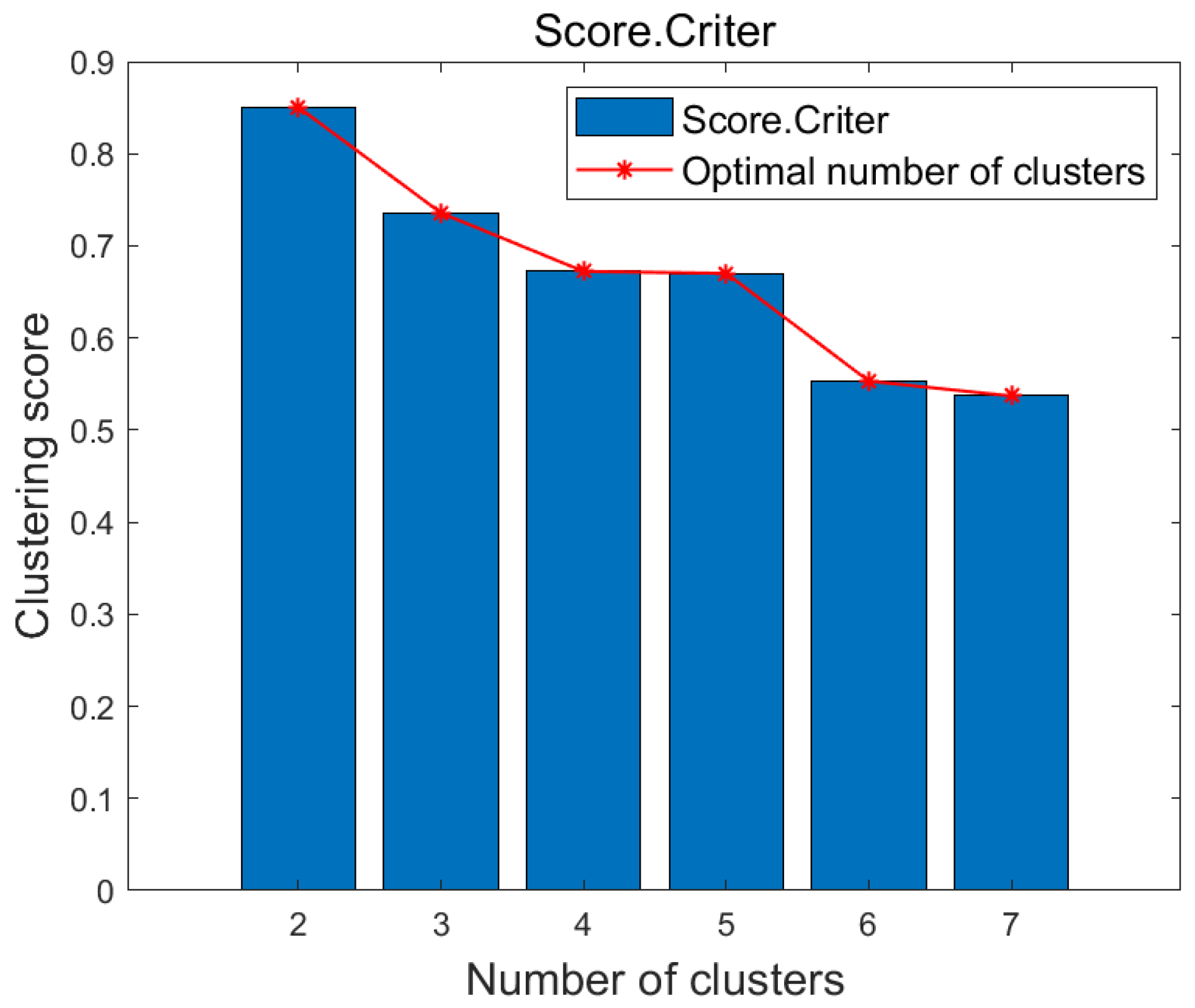
The appropriate number of clusters is the key to obtain the optimal clustering results. When the number of clusters is large, the clustering results are more accurate, and the intra-class relationship is more compact, but the results are more complex. When the number of clusters is small, the clustering results are saved in a certain error. Figure 13 shows a number of clustering performance indicators corresponding to different number of clusters, including Score.DBvalue (DB), Score.CriterionValues (CH), and so on.
The DB is evaluated based on the closeness within the cluster and the separation between clusters. The value range of DB is that the smaller the value, the better the clustering effect, that is, the data points within the cluster are closer, and the data points between different clusters are more dispersed. The following are the calculation steps for the DB.
R i j = S i + S j z i z j
D B = 1 c i , j = 1 c max i j R i j
Where R i j is the similarity relationship between the i-th cluster and the j-th cluster, S i is the intra-cluster diameter of the i-th cluster, representing the average distance between all sample points in the i-th cluster and the center of the corresponding cluster, and z i z j is the distance between two clusters. For the similarity R i j of the i th cluster, the DB is equal to the maximum value in R i 1 , R i 2 R i j ; for the overall sample data, the DB is the average of all cluster similarities. It can be seen from the figure that as the number of clusters increases, the DB index gradually increases, especially when the number of clusters is greater than 4. This indicates that the poor separation between classes may be due to the forced allocation of more categories. The index reaches the lowest value when the number of clusters is 2, indicating that the clustering results have the best intra-class tightness and inter-class separation.
The essence of CH is the ratio of inter-cluster distance to intra-cluster distance, and the overall calculation process is similar to the variance calculation method, also known as the variance ratio criterion. As shown in the figure, the CH performs higher when the number of clusters is 1 and 2. When the number of clusters is greater than 3, the CH index decreases significantly, indicating that the separation between classes is poor, the tightness within the class is insufficient, and the clustering results begin to deteriorate.
The Silhouette Coefficient is an index used to evaluate the quality of clustering results. It combines the tightness within each data point cluster and the separation between clusters, denoted as s ( i ) . The formula is as follows:
s ( i ) = b ( i ) a ( i ) max ( a ( i ) , b ( i ) )
a ( i ) is the average distance between each data point and all other points in the cluster, and b ( i ) is the average distance between each data point and all points in the nearest neighbor cluster. When the s ( i ) value is close to 1, the separation between classes is very good, and the clustering effect is excellent. When the s ( i ) value is close to 0 or even becomes negative, the separation between classes is blurred, the data points may be misallocated to other classes, and the clustering effect is poor. It can be seen from Figure 14 that when the number of clusters is 2, the contour coefficient reaches the peak value, which is close to 0.9, indicating that the clustering results have the best intraclass tightness and inter-class separation. When the number of clusters is greater than 4, the contour coefficient decreases significantly; when the number of clusters is 6 or 7, the contour coefficient is less than 0.6, which indicates that the clustering quality decreases at this time, and there may be excessive clustering or fuzzy boundaries between classes.
In summary, this study employs multiple clustering evaluation metrics, including the Davies–Bouldin index (DB), Calinski–Harabasz criterion (CH), and the Silhouette Coefficient, to comprehensively assess the clustering performance under different numbers of clusters. The results show that when the number of clusters is 2, the DB index reaches its minimum value, indicating optimal intra-cluster compactness and inter-cluster separation. Simultaneously, both the CH index and the Silhouette Coefficient achieve their peak values at c = 2 , reflecting strong class separability and structural stability. Therefore, based on the trend and quantitative results of these evaluation metrics, it can be concluded that selecting c = 2 as the number of clusters yields the most effective and reliable clustering outcome for the given data set. This choice helps avoid over-clustering and ensures clear class boundaries, thus enabling accurate classification of multi-dimensional data.

4.4. Radial Basis Function Neural Network

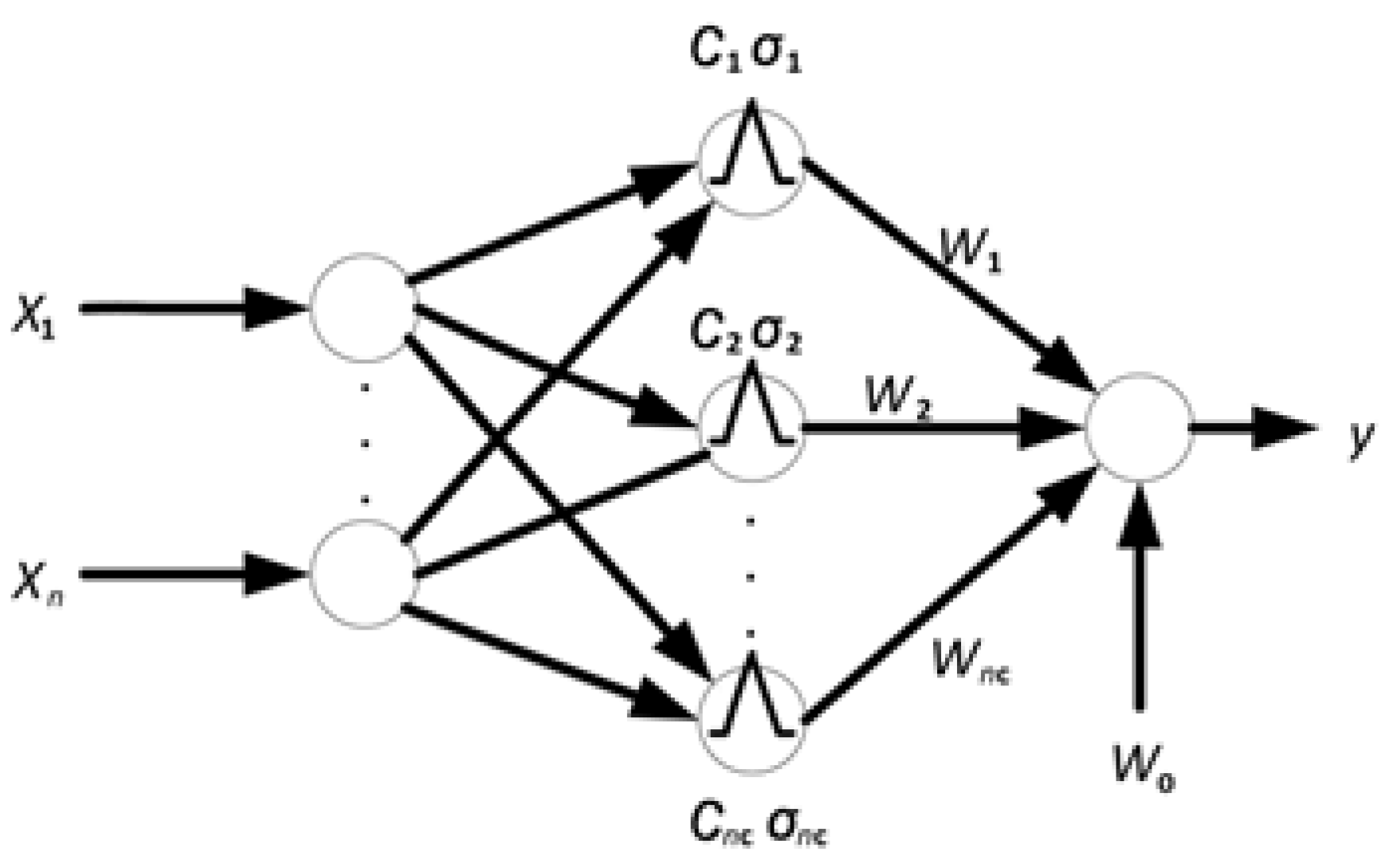
As shown in Figure 15, RBF neural network is a three-layer feed-forward network, which has a simple structure and strong nonlinear approximation ability. It has a wide range of applications in solving nonlinear regression and classification problems. Input layer to hidden layer mapping:
ϕ ( x c n ) = exp x c n 2 2 σ n 2
Linear weighted mapping from hidden layer to output layer:
y ( x ) = n = 1 c w n ϕ ( x c n ) + e
The input x is the cluster sample of the total pressure recovery coefficient of the inlet; σ n is extended width factor; w n represents the connection weight from the hidden layer to the output layer, and e is the output bias, The hidden layer nodes adopt RBF activation function; c n is the center position of the hidden layer node. c is the number of hidden layer nodes, that is, the number of clusters obtained by the above analysis.

4.5. NDAPSO-RBF Neural Network

For the traditional RBF neural network, the extended width factor σ n determines the response range of the neuron. Too many hidden layer nodes lead to over-fitting, and too few reduce the approximation ability. In view of these two aspects, this study establishes a two-level dynamic optimization mechanism by combining FCM clustering optimization and adaptive PSO algorithm: using FCM clustering to select the optimal clustering number c = 2 . The NDAPSO dynamic optimization nonlinear inertia weight w is designed to search for the best expansion width factor σ n b e s t .
The number of hidden layer nodes of RBF neural network is determined by the optimal clustering number of FCM. By evaluating the contour coefficient (as shown in Figure 14), it is observed that when the clustering number c = 2 , the contour coefficient reaches the peak, indicating that the clustering effect is optimal at this time. Therefore, the number of hidden layer nodes in the RBF neural network is set to 2 to ensure that the distribution of hidden layer nodes is highly matched with the clustering center of sample feature space, which not only avoids over-fitting, but also fully retains the approximation ability of the model to nonlinear features.
The optimization of the extended width factor σ n is realized by NDAPSO algorithm: the nonlinear inertia weight strategy is designed by Equations (10)–(15). At the beginning of the iteration ( 0 t 0.3 T max ), the high nonlinear inertia weight w value is maintained to enhance the global search ability, and at the later stage ( 0.7 T max < t T max ), nonlinear inertia weight w is reduced to improve the local fine-tuning accuracy, and the population convergence state is monitored in real time. When the sudden increase of nonlinear inertia weight w is detected, the sinusoidal disturbance term is activated to force the particles to jump out of the local optimal region.
In order to further evaluate the global search ability of each algorithm, this paper records the success rate comparison table shown in Table 4 and counts the proportion of each algorithm successfully reaching the preset error threshold ( M S E < 1 × 10 3 ) in 100 times. The results show that the success rate of NDAPSO is as high as 92%, which is better than other methods, showing its strong ability to jump out of local optimum. BP-PSO also performs well, which combines neural network gradient to guide search, making it easier for particles to converge to the target area. In contrast, the traditional PSO has a lower success rate than NDAPSO, especially under the fixed inertia factor (such as b = 0.8) strategy, indicating that improper parameter setting will seriously affect the robustness and reliability of the algorithm.
At the same time, in order to verify the generalization ability of the model in this paper, four different data sets are used by setting different inlet geometric angles and fluid simulation conditions, as shown in the following Table 5.
The optimization objective is to minimize the root mean square error (RMSE) of the network:
RMSE = i = 1 n ( y i y ^ i ) 2 n
The experimental results show that the NDAPSO-RBF neural network shows excellent prediction accuracy and generalization ability on both the training set and the test set. From the comparison diagram of the prediction results of the training set (Figure 16), it can be seen that the true value and the predicted value are almost completely coincident, and the root mean square error RMSE is 3.8108 × 10 8 . This shows that the NDAPSO-RBF neural network has a high fitting ability to the training set data and can accurately capture the complex nonlinear relationship between input and output. This is due to the dual optimization mechanism of hidden layer nodes: On the one hand, the optimal number of hidden nodes c = 2 determined by the sample data set is processed by FCM clustering, which makes the radial basis function accurately cover the high-density area of the sample and avoid the feature mismatch caused by traditional random initialization. On the other hand, the NDAPSO algorithm’s fine-tuning of the extended width factor σ n significantly improves the adaptability of the basis function boundary.
In the comparison diagram of the prediction results of the test set, RMSE is 8.2609 × 10 8 (compared with the training set, the error of the test set is increased by 53 % ), and 98.3% of the predicted values in the scatter plot are distributed in the y = x ± 3 β interval ( β = 1.2 × 10 7 ), indicating that the model has strong generalization ability. At the same time, the two-stage search strategy of NDAPSO expands the range of parameter search and effectively avoids the local convergence trap of traditional PSO algorithm through the synergistic effect of early global exploration and later local oscillation.
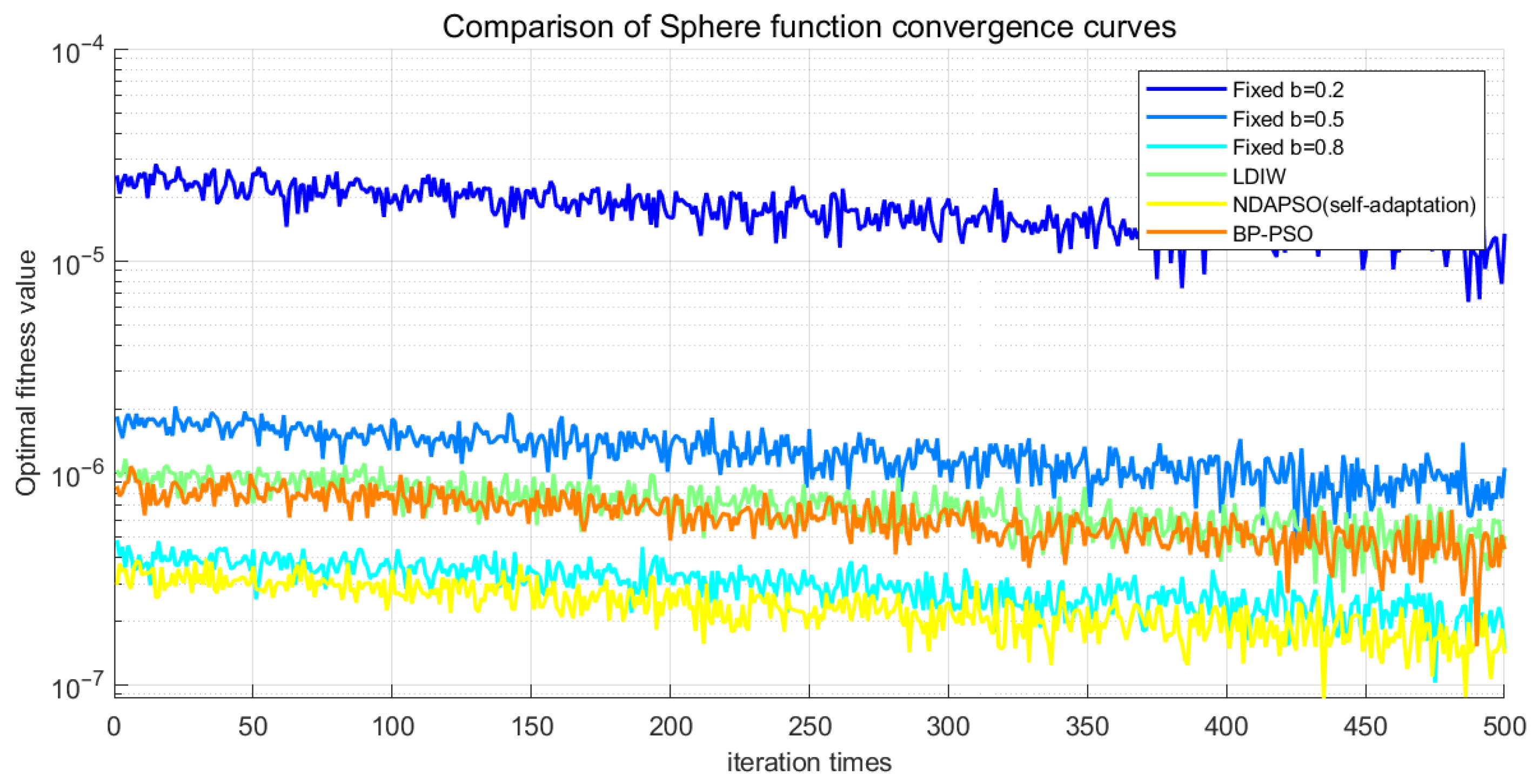
It can be seen from the convergence curve of the Sphere function (Figure 17) that NDAPSO and BP-PSO show good convergence speed and final accuracy in the whole optimization process. Among them, NDAPSO has a significant decline advantage in the early search stage and converges to the global optimum in the later stage, indicating that its adaptive mechanism can effectively balance the search and development capabilities. BP-PSO benefits from the fine-tuning ability of BP algorithm and performs well in error correction in the middle and late stages. In contrast, the Fixed b series strategies perform generally in terms of convergence speed and final accuracy, and the fixed inertia weight may limit their search flexibility.
In order to test the efficiency of various algorithms in this paper, a double cuboid model is used for testing. The underground space is further divided into 20 × 20 × 20, 30 × 30 × 20, 40 × 40 × 20 and 50 × 50 × 20 grids, and the performance of the algorithm in the different cases is compared. Table 6 records the most efficient value, and calculates the speedup ratio.
From the statistical results (Table 6), it can be seen that with the increase in grid size, the improved NDAPSO algorithm has obvious advantages in calculating large-scale grid data, and the acceleration ratio shows an increasing trend. But when the number of grids increases to 50 × 50 × 20, the speedup ratio begins to decrease. The reason may be that it takes a certain amount of time for data to be transmitted from the CPU to the GPU, and the increase in the number of grids leads to an increase in transmission time, which affects the acceleration efficiency.
Figure 18 shows the number of function calls and its standard deviation required by different algorithms in the optimization process to evaluate their computational cost and stability. It can be seen that NDAPSO has the lowest number of function calls and the lowest standard deviation, indicating that it achieves a good balance between accuracy and efficiency. BP-PSO comes second in performance, and it also has strong generalization ability while maintaining stability. In contrast, the traditional PSO with fixed parameters (especially b = 0.8) not only requires more computing resources, but also fluctuates significantly, indicating that it lacks global control ability and is easy to fall into the inefficient local search stage.
In order to ensure the fairness and reproducibility of the experiment, this paper tests and compares all algorithms in a unified computing environment. All simulation experiments are run independently on the local computing platform, and the related hardware and software configurations are shown in Table 7. Each algorithm runs 100 times under the same configuration conditions to count its average performance index and volatility (standard deviation or confidence interval). In addition, in order to reduce the impact of accidental errors on the evaluation results, all data are taken as the statistical average of multiple independent operations. Finally, the configuration of the simulation platform is given.

5. Conclusions

This study introduces a novel FCM-NDAPSO-RBF neural network framework to model and predict the aerodynamic performance of S-shaped inlets, aiming to overcome the computational bottlenecks and empirical dependencies associated with traditional CFD simulations. By applying FCM clustering directly to the output parameter—total pressure recovery coefficient σ —the model effectively captures the physical distribution features critical for aerodynamic optimization. Furthermore, the NDAPSO algorithm dynamically adjusts the inertia weight in three evolutionary stages, enhancing both global search efficiency and local fine-tuning precision. Quantitative evaluations show that the proposed model achieves high predictive accuracy, with RMSE as low as 3.81 × 10 8 in training and 8.26 × 10 8 in testing. It demonstrates a 92 % success rate in convergence under stringent error thresholds and achieves the least number of function calls and the lowest standard deviation compared to conventional PSO-RBF methods, indicating that it achieves a good balance between accuracy and efficiency. The clustering process also reduces the dimensionality of feature inputs, improving parameter tuning efficiency. These results affirm the feasibility of the model as a data-driven surrogate method for real-time, multi-condition aerodynamic prediction and stealth optimization.
However, some limitations remain. First, the current model assumes static inlet geometry and does not account for real-time deformation or dynamic boundary conditions during flight. Second, the generalization capability, although promising, still requires validation on more diversified data sets including high-fidelity experimental wind tunnel data. Third, the interpretability of the model decisions, typical of neural network-based approaches, is limited and requires further explainability enhancement for engineering integration.
Future research will focus on extending this method to time-varying flow conditions, integrating physics-informed neural networks to incorporate prior aerodynamic knowledge, and combining the model with real-time optimization frameworks for adaptive inlet shape design under variable stealth and performance constraints.

Author Contributions

Conceptualization, L.X.; methodology, Y.W. and L.X.; software, Y.W. and X.Z.; validation, Y.W.; formal analysis, Y.W. and J.H.; investigation, Y.W.; resources, L.X.; data curation, Y.W., X.Z., J.H. and J.L.; writing—original draft preparation, Y.W.; writing—review and editing, Y.W.; visualization, Y.W.; supervision, L.X.; project administration, L.X.; funding acquisition, L.X. and J.L. All authors have read and agreed to the published version of the manuscript.

Funding

This manuscript supported by Jiangsu Province Frontier Technology Research and Development Program (BF2024023) and National Natural Science Foundation of China (No.62373185).

Data Availability Statement

The data presented in this study are available in article (pictures, charts, etc.)

Acknowledgments

The authors would like to thanks all of lab-mates. This work is partially supported by High Performance Computing Platform of Nanjing University of Aeronautics and Astronautics.

Conflicts of Interest

The authors declare no conflicts of interest.

List of Symbols

σ Total pressure recovery coefficient
P 1 * Total pressure of the outlet airflow of the inlet
P 0 * Total pressure of the free unperturbed airflow
P 1 * max The maximum value of the total pressure of the airflow at the outlet section of the inlet
P 1 * min The minimum value of the total pressure of the airflow at the outlet section of the inlet
P ¯ 1 * The average total pressure of the total area of the inlet outlet
D ¯ The distortion coefficient
QThe air quality flow
ρ The fluid density
AThe size of the corresponding cross-sectional area
y h The longitudinal coordinate of center line of the diffuser
HThe longitudinal offset of the diffuser
x h The transverse coordinate of the diffuser centerline
L d i f f The length of the diffuser
A 1 The inlet area of the diffuser
A 2 The outlet area of the diffuser.
p b e s t The individual optimal solution
g b e s t The global optimal solution
v i k The velocity of the particle i at the iteration k
wInertia weight in PSO
c 1 , c 2 Learning factor
r 1 , r 2 Random numbers
p b e s t i k The individual optimal position of the particle i
g b e s t i k The globa optimal position of the particle i
p i k The position of the particle i at the iteration k
ω The fixed inertia weight
ω ( t ) The time-varying inertia weight
ω max , ω min The maximum and minimum inertia weights
T max The maximum number of iterations
tThe current number of iterations
k ( t ) The population evolution fitness index function
S t d F i t ( t ) The standard deviation of the fitness of the current population particles
N 0 , 0 . 05 2 The random disturbance term
N ( 0 , 1 ) The random disturbance term
M ( 0 , 1 ) The random disturbance term
DThe goodness of fit between the particle position distribution and the normal distribution
S ( x ) The nonlinear feature mapping activation function
bThe fixed adaptation factor
Δ wAmplitude
gGlobal best position
b ( t ) The time-varying adaptation factor
RThe diffusion radius
E later The later oscillation energy
E mid - term The medium-term oscillation energy
BThe sample data
x k * The clustering sample before normalization
x m i n * The minimum value in the clustering sample
x m a x * The maximum value in the clustering sample
x k The normalized clustering sample
y ^ i The inverse normalized predictive value
y ^ * i The normalized predictive value
JThe objective function
cThe number of clusters
mThe fuzzy coefficient
u i j The membership degree of the sample j in the class i
d i j The central distance between the two points of the sample j and the cluster center i
f i Input contraction mapping
z i The cluster center
λ k modulus
R i j The similarity relationship between the i-th cluster and the j-th cluster
S i The intra-cluster diameter of the i-th cluster
D B The average of all cluster similarities
s ( i ) The tightness within each data point cluster and the separation between clusters
a ( i ) The average distance between each data point and all other points in the cluster
b ( i ) The average distance between each data point and all points in the nearest neighbor cluster
ϕ RBF activation function
σ n The extended width factor
ω n The connection weight from the hidden layer
c n The center position of the hidden layer node
eThe output bias
β Diffusion interval
FCMFuzzy C-Means
PSOParticle Swarm Optimization
NDAPSONonlinear Dynamic Adaptive Particle Swarm Optimization
RBFRadial Basis Function
RBFNNRadial Basis Function Neural Network
RMSERoot Mean Square Error
RANSReynolds Averaged Navier–Stokes Equation
AMPCAdaptive Model Predictive Control
LDIWLinear Decreasing Control Strategy
DBDB Value
CHCriterionValue

References

  1. Xiang, G.; Hong, Z.; Wenjian, D.; Jiaqi, W. Investigation of Aerodynamic and Electric Scattering Characteristics of Double S-shaped Intake with Different Inlet Shapes. Comput. Simul. 2018, 35, 35–39. [Google Scholar]
  2. Zeng, L.; Hu, J.; Pan, D.; Li, J.; Shao, X. Multi-points and multi-objective optimization design of subsonic UAV S-shaped inlet. J. Propuls. Technol. 2021, 42, 495. [Google Scholar]
  3. Liu, X.; Liu, W.; Zhao, Y. Navier–Stokes predictions of dynamic stability derivatives for air-breathing hypersonic vehicle. Acta Astronaut. 2016, 118, 262–285. [Google Scholar] [CrossRef]
  4. Belaidouni, H.; Samardžić, M.; Živković, S.; Kozić, M. Computational fluid dynamics and experimental data comparison of a missile-model roll derivative. J. Spacecr. Rocket. 2017, 54, 672–682. [Google Scholar] [CrossRef]
  5. Ronch, A.D.; Vallespin, D.; Ghoreyshi, M.; Badcock, K. Evaluation of dynamic derivatives using computational fluid dynamics. AIAA J. 2012, 50, 470–484. [Google Scholar] [CrossRef]
  6. Liu, J.; Li, C.; Teng, P.; Tang, B.; Cao, Y. Actual-Calibration Technique of Gas Flowmeters in Inlet Wind Tunnel Test. J. Propuls. Technol. 2023, 44, 174. [Google Scholar] [CrossRef]
  7. Wang, Z.; Zhao, Y. Data-driven exhaust gas temperature baseline predictions for aeroengine based on machine learning algorithms. Aerospace 2022, 10, 17. [Google Scholar] [CrossRef]
  8. Liu, Y.; Chen, J.; Cheng, J.; Xiang, H. Aerodynamic optimization of transonic rotor using radial basis function based deformation and data-driven differential evolution optimizer. Aerospace 2022, 9, 508. [Google Scholar] [CrossRef]
  9. Zhang, Y.; Zheng, H.; Xu, J.; Wang, Z. Radial basis function model-based adaptive model predictive control for trajectory tracking of a clapping-wing micro air vehicle. Aerospace 2023, 10, 253. [Google Scholar] [CrossRef]
  10. Wei, J.; Zheng, Q.; Yan, W.; Jiang, B. Dynamic particle swarm optimization-radial function extremum neural network method of HCF probability analysis for compressor blade. Int. J. Fatigue 2023, 176, 107900. [Google Scholar] [CrossRef]
  11. Wu, Y.; Sun, G.; Tao, J. An improved multi-objective particle swarm optimization method for rotor airfoil design. Aerospace 2023, 10, 820. [Google Scholar] [CrossRef]
  12. Shi, Y.; Eberhart, R. A modified particle swarm optimizer. In Proceedings of the 1998 IEEE International Conference on Evolutionary Computation Proceedings, IEEE World Congress on Computational Intelligence (Cat. No. 98TH8360), Anchorage, AK, USA, 4–9 May 1998; pp. 69–73. [Google Scholar]
  13. Li, R.; Guo, Y.; Nguang, S.K.; Chen, Y. Takagi-Sugeno fuzzy model identification for turbofan aero-engines with guaranteed stability. Chin. J. Aeronaut. 2018, 31, 1206–1214. [Google Scholar] [CrossRef]
  14. Pan, M.; Wang, H.; Huang, J. T–S Fuzzy Modeling for Aircraft Engines: The Clustering and Identification Approach. Energies 2019, 12, 3284. [Google Scholar] [CrossRef]
  15. Zheng, R.; Qi, K.; Zhang, Q.; Xiao, Z.; Liu, H. Integrated investigation of aerodynamic shape and stealth performance for supersonic vehicle with “X” sawtooth lip inlet. J. Propuls. Technol. 2017, 38, 2471. [Google Scholar]
  16. Yu, X.; Zhao, M. A study on stealth technology in UAV inlet design. Flight Dyn.-Xian 2007, 25, 69. [Google Scholar]
  17. Shi, L.; Guo, R. Electromagnetic scattering of a submerged inlet. Acta Aeronaut. Et Astronaut. Sin. 2008, 29, 1098–1104. [Google Scholar]
  18. Lee, C.; Boedicker, C. Subsonic diffuser design and performance for advanced fighter aircraft. In Proceedings of the Aircraft Design Systems and Operations Meeting, Colorado Springs, CO, USA, 14–16 October 1985; p. 3073. [Google Scholar]
  19. Zhang, J.; Zhan, H.; Mi, B. Study on Aerodynamic Design of the Front Auxiliary Inlet. Aerospace 2023, 10, 700. [Google Scholar] [CrossRef]
  20. Jia, W.; Li, G.; Liu, T.; Kong, Q.; Ding, S. Numerical Analysis of the Effect of S-Shaped Duct Key Geometry Parameters on the Inlet Distortion of Distributed Ducted Fans. Aerospace 2025, 12, 316. [Google Scholar] [CrossRef]
  21. Zhang, L.; Zhou, Z.; Xu, X. Area and centerline distribution on stealth design of S-shaped inlet. J. Syst. Simul. 2019, 30, 2999–3006. [Google Scholar]
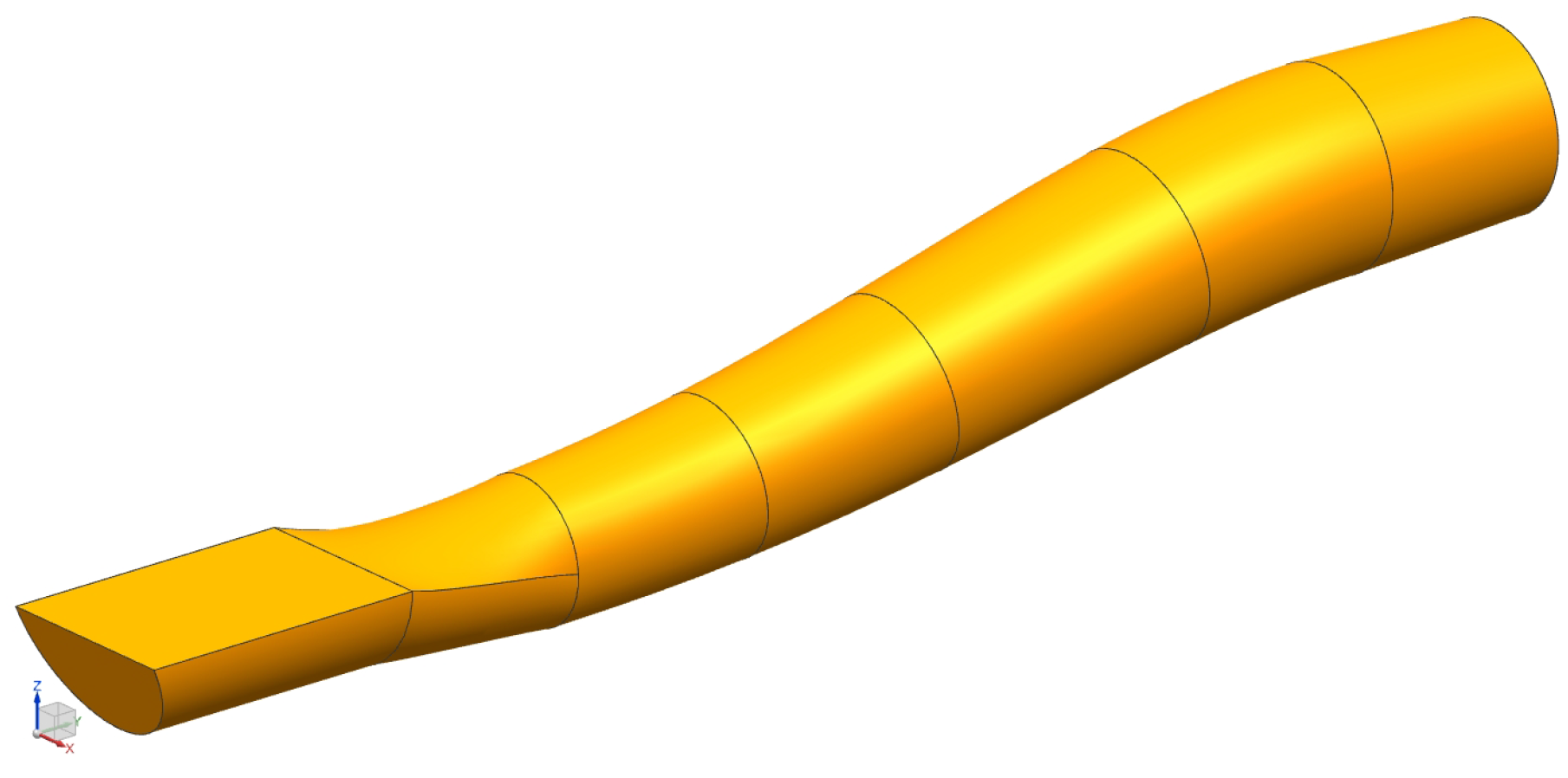
Figure 1. The overall structure of the S-shaped inlet.
Aerospace 12 00748 g001
Figure 2. The intake section of the S-shaped inlet.
Aerospace 12 00748 g002
Figure 3. The diffuser section of the S-shaped inlet.
Aerospace 12 00748 g003
Figure 4. The exit section of S-shaped inlet.
Aerospace 12 00748 g004
Figure 5. The standard deviation of dynamic fitness.
Aerospace 12 00748 g005
Figure 6. Stage 1: Global exploration.
Aerospace 12 00748 g006
Figure 7. Stage 2: Medium-term transition.
Aerospace 12 00748 g007
Figure 8. Stage 3: Sensitive fluctuation.
Aerospace 12 00748 g008
Figure 9. The improved stage 1: Global exploration.
Aerospace 12 00748 g009
Figure 10. The improved stage 2: Medium-term transition.
Aerospace 12 00748 g010
Figure 11. The improved stage 3: Sensitive fluctuation.
Aerospace 12 00748 g011
Figure 12. Historical data of total pressure recovery coefficient of inlet.
Aerospace 12 00748 g012
Figure 13. Finding the best number of clusters.
Aerospace 12 00748 g013
Figure 14. Score.Silhouette Coefficient.
Aerospace 12 00748 g014
Figure 15. Radial basis function neural network.
Aerospace 12 00748 g015
Figure 16. RBF neural network prediction results.
Aerospace 12 00748 g016
Figure 17. Comparison of Sphere function convergence curves.
Aerospace 12 00748 g017
Figure 18. Comparison of Computational Cost (Function Calls).
Aerospace 12 00748 g018
Table 1. The early characteristic value of dynamic inertia weight.
ParameterAverage Diffusion RadiusPeak CoverageAttenuation Rate of Inertia Weight
b = 0.8 5.21 8.7 % 7.6 %
b = 0.5 4.05 5.3 % 11.2 %
b = 0.2 2.89 3.1 % 18.4 %
L D I W 4.23 6.1 % 9.8 %
Table 2. The mid-term characteristic value of dynamic inertia weight.
ParameterConvergence PrecisionMulti-Peak Success RateDisturbance
b ( t ) 3.27 × 10 27 92.4 % 0.12
b = 0.5 1.76 × 10 6 78.9 % 0.17
Table 3. The late characteristic value of dynamic inertia weight.
ParameterConvergence PrecisionPeak CoverageDisturbance
b = 0.8 2.91 × 10 3 51.6 % 0.03 ± 0.01
b = 0.5 1.76 × 10 6 78.9 % 0.07 ± 0.03
b = 0.2 4.13 × 10 7 62.3 % 0.15 ± 0.06
L D I W 9.83 × 10 7 71.2 % 0
Table 4. Operation records of different algorithms.
AlgorithmNumber of SuccessesNumber of Failures
N D A P S O 928
B P P S O 8614
b = 0.2 6414
b = 0.5 7129
b = 0.8 5149
L D I W 6832
Table 5. Description of benchmark data sets.
Number of Mesh UnitsSample NumberCharacteristic Number
20 × 20 × 20 35134
30 × 30 × 20 37330
40 × 40 × 20 56957
50 × 50 × 20 68370
Table 6. The running time statistics of different prediction methods.
Traditional PSO-BP/sTraditional PSO-RBF/sNDAPSO-RBF/sSpeed-Up Ratio
3.630 3.652 3.231 1.13
16.117 16.126 13.258 1.216
49.462 49.577 45.865 1.081
122.563 124.781 120.927 1.032
Table 7. Simulation experiment computing platform configuration.
ItemConfiguration Parameter
Operating systemWindows 11 64-Bit
CPUIntel Core i7-12700H (14 Cores, 20 Threads, 2.3 GHz) (Intel, Santa Clara, CA, USA)
RAM16 GB DDR4 3200 MHz
GPUNVIDIA RTX 3070 GPU (NVIDIA, Santa Clara, CA, USA)
Programming language/environmentMATLAB R2023a/Python 3.10 + NumPy/SciPy/PyTorch
Simulation algorithm running environmentMATLAB built-in function + custom function
(PSO, NAPSO, BP-PSO module)
Disclaimer/Publisher’s Note: The statements, opinions and data contained in all publications are solely those of the individual author(s) and contributor(s) and not of MDPI and/or the editor(s). MDPI and/or the editor(s) disclaim responsibility for any injury to people or property resulting from any ideas, methods, instructions or products referred to in the content.