A Versatile UAS Development Platform Able to Support a Novel Tracking Algorithm in Real-Time

Abstract

A primary objective of this research entails the development of an innovative algorithm capable of tracking a drone in real-time. This objective serves as a fundamental requirement across various applications, including collision avoidance, formation flying, and the interception of moving targets. Nonetheless, regardless of the efficacy of any detection algorithm, achieving 100% performance remains unattainable. Deep neural networks (DNNs) were employed to enhance this performance. To facilitate real-time operation, the DNN must be executed within a Deep Learning Processing Unit (DPU), Neural Processing Unit (NPU), Tensor Processing Unit (TPU), or Graphics Processing Unit (GPU) system on board the UAV. Given the constraints of these processing units, it may be necessary to quantify the DNN or utilize a less complex variant, resulting in an additional reduction in performance. However, precise target detection at each control step is imperative for effective flight path control. By integrating multiple algorithms, the developed system can effectively track UAVs with improved detection performance. Furthermore, this paper aims to establish a versatile Unmanned Aerial System (UAS) development platform constructed using open-source components and possessing the capability to adapt and evolve seamlessly throughout the development and post-production phases.

1. Introduction

Object tracking is a fundamental task in image processing with many applications in fields like robotics, autonomous vehicles, surveillance, and human–computer interaction. The goal of object tracking is to identify and monitor the position of a target in a sequence of video frames, despite the difficulties generated by occlusions, different types of variabilities and variances, illumination changes, weak contrast, motion blur, and background clutter.

In several types of unmanned aerial vehicle (UAV) guidance, object tracking is a primary requirement of the algorithm [1,2]. Primarily, guidance is the process of controlling the trajectory, or the path of a UAV, to a given point (the goal) based on several constraints, such as the shortest route, obstacle avoidance, and consumption optimization, among others. One of the primary goals of the various autopilots (PX4, ArduPilot, or INAV) is to guide the UAV along a predefined trajectory, based on GPS information [3,4]. Furthermore, various UAV systems employ alternative guidance systems that facilitate target tracking [5,6] to enable (1) maneuvering within a defined formation for multiple UAVs, (2) following and intercepting a moving system, or (3) avoiding potential collisions.

The most used and effective guidance laws for different UAV systems, designed to track a target, are the pure pursuit guidance law and the proportional navigation guidance law [2,6,7].

In the pure pursuit (PP) guidance law [2], the velocity vector of the follower UAV always heads to a point on the trajectory of the target (named lookahead point) that is ahead of the current position of the target but on the vehicle’s path or even in the line with the actual target position. Therefore, the direction of the velocity vector must be in line of sight (LOS) between the follower (the tracker) system and the lookahead point. The LOS is the direct line between the tracker and the target.

The guidance systems based on the proportional navigation law have several implementations [2,7], including pure proportional navigation (PPN), true proportional navigation (TPN), augmented proportional navigation (APN), optimal guidance law (OGL) or proportional navigation with optimal gain—to name only the most important proportional navigation laws.

There are several methods used in UAV detection based on [8,9]: (a) thermal detection, (b) the scanning and detection of radio frequency signals, (c) radars, (d) optical cameras, (e) acoustic signal detection, and (f) hybrid methods that use a combination of these methods.

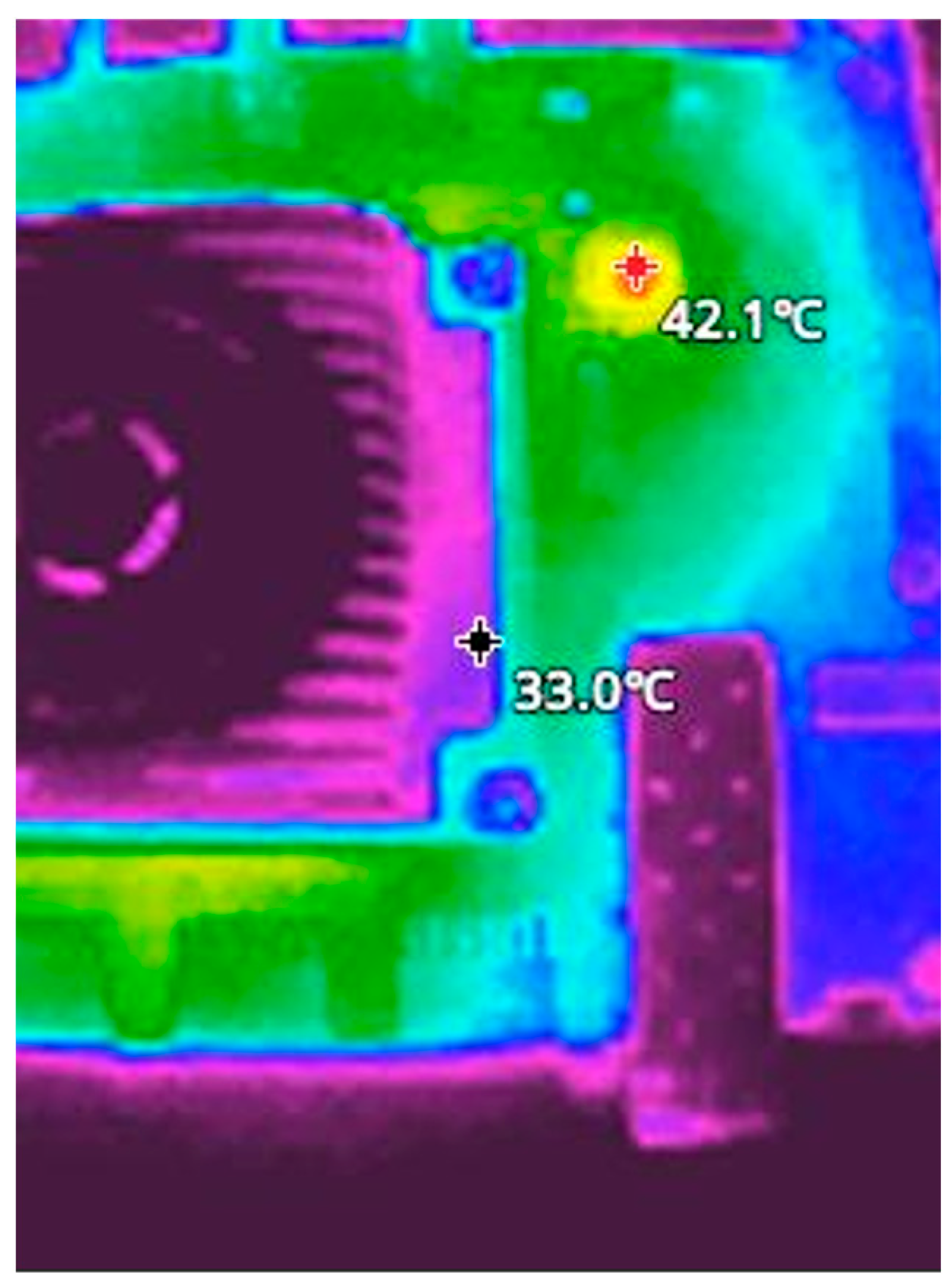
Thermal UAV detection is based on the heat generated by different components placed on the UAV [8,9]. Especially motors, as well as components such as batteries, internal processors, or other internal electrical or electronic devices generate heat. In more complex approaches, even panoramic thermal image sensors are used [10].

Each UAV system exchanges information through different radio frequency (RF) channels [8,9,11]. The RF connections between the UAV and the ground control (remote control signals, video links, telemetry information, etc.) represent one of the vulnerabilities of these systems that can be exploited for their detection. However, detecting UAVs through the RF-generated signals is considered a complex operation because, in general, the different working bands of UAV systems are crowded with noise and other signal sources that generate many signals. To address this issue, [11] proposes a hierarchical approach that utilizes four classification systems, operating under an ensemble concept. By following this approach, the developed system can detect even the flight mode of the UAV, including hovering and flying.

Despite being the most expensive method of UAV detection, radar systems are used for this purpose [8,9], even though these have small radar cross-sections (RCS) and, as a direct result, are difficult to detect [12]. Analyzing three types of radars, based on experimental and theoretical results, it was demonstrated that Frequency-Modulated Continuous-Wave (FMCW) radars are the most suitable for detecting and tracking small RCS targets, such as UAVs [12].

The utilization of the audio signal generated by the motors of a UAV constitutes an alternative method cited in the literature [8,9] for detecting a UAV. The main disadvantage of this method is its minimal detection range. Furthermore, accurately determining the distance to the drone and identifying the direction from which the sound emanates pose two additional significant challenges to a precise estimation of the 3D position [8]. The literature examines the detection of UAVs based on acoustic signals through two methodologies [13]: (a) a one-dimensional analysis focusing on the magnitude or phase of the sound sources, and (b) a two-dimensional analysis examining the spectrogram of the acoustic signals. Using the second approach and a custom deep neural network with 10 layers, the researchers from [13] achieved a 97% accuracy with an error rate of 0.05, maintaining a distance of 3 m between the drone and the microphones. However, the paper notes that the most significant factor limiting accuracy is the distance between the drone and the microphones.

The final method, which involves the detection and tracking of UAVs, utilizes an optical camera. This approach was adopted during this research.

Using an image or several images, traditional object detection and tracking approaches include (a) template matching-based methods [14]; (b) feature extraction, such as a histogram of oriented gradients (HOG) followed by a classical classification algorithm (ensemble learners trained with the AdaBoost algorithm) [15,16]; (c) Haar features [16]; (d) knowledge-based methods [14]; (e) optical flow [17]; (f) a clustering algorithm and a Support Vector Machine (SVM) classifier [18]; and (g) object-based image analysis (OBIA) for object detection [14]. These classical approaches have demonstrated effective outcomes in constrained environments; however, they encounter significant challenges when applied to complex real environments.

Recent advancements in deep learning, especially in convolutional neural networks (CNNs) and transformer-based architectures, have significantly improved detection accuracy. Deep neural network (DNN) object detection algorithms are divided into two main classes: (1) one-stage (e.g., You Only Look Once (YOLO) [19,20], SSD [21], RetinaNet [22], DETR [23,24]), and (2) two-stage (e.g., R-CNN [25], Faster R-CNN [26], SPP-Net [27], Feature Pyramid Network (FPN) [28]).

The accuracy of DNN systems has been improved through various approaches.

In the first approach, different research teams have proposed different and novel conceptual strategies for object detection. This has led to the emergence of new architectures, such as SSD [21], DETR [23], or YOLO [29]. For instance, for the first time, YOLO treats the detection as a single step in a unified detection paradigm [29]. In another architecture, DETR treats object detection as a prediction problem that enforces unique predictions through a bipartite matching strategy [23].

In the second approach, the existing architectures were continuously refined and improved to achieve superior performance. This is the case with the YOLO architecture, which, since its launch in 2016, YOLOv1 [29], has undergone numerous variants, reaching YOLOv12 in 2025 [30]. In this area, progress has continued to advance even further. Starting with an architecture like YOLOv5, as described in [31], modifications are introduced by adding an ESTDL (Efficient Small Target Detection Layer) and a new bottleneck structure (MLCSP) to enhance feature representation. Ultimately, a new detection algorithm, YOLO-LSM, has emerged as a lightweight UAV target detection algorithm [31]. In another study [32], the framework YOLO-DCTI is proposed for the remote sensing of small or tiny object detection, such as UAVs. YOLO-DCTI is based on YOLOv7 and a new improved Context Transformer (CoT-I) block.

In the third approach, in addition to the main detection algorithm, other algorithms are employed to enhance detection performance. For instance, in [33], a YOLOv5 algorithm enhanced with time-domain information, acquired through a Kalman filter, demonstrated improved detection performance.

This paper addresses the following question: How can a deep neural network tracking algorithm (powerful but with high computational requirements) be optimized and improved to meet the conflicting requirements of working in real-time in an embedded unit while enhancing detection performance and maintaining its computational efficiency?

The hypothesis examined in this study proposes that the above question can be positively addressed through the incorporation of a deep neural network (DNN)-based detection mechanism within a synergistic algorithmic framework. This framework is optimized for embedded hardware environments and supported by DPU and CPU units. Consequently, improved real-time drone tracking performance can be achieved despite computational constraints, while simultaneously promoting the development of a versatile open-source unmanned aerial system (UAS) platform.

The novel algorithm presented in this paper is based on a similar approach to the one presented above [33]. The novel object tracking framework addresses the challenge of missed detection. The new algorithm is based on a DNN-type neural network, specifically a YOLO-type network, and its performance is enhanced by utilizing spatial correlation information (provided by a correlation tracking algorithm) along with temporal information provided by a Kalman filter. Ultimately, this approach yields superior detection results. The methodology was evaluated using a publicly accessible dataset collected during this research, demonstrating its effectiveness compared to existing techniques.

The remainder of this paper is organized as follows: Section 2 presents the materials and methods employed in this research, including the UAV system that supports the algorithm, the database used, and the algorithms utilized. In Section 3, the results obtained are discussed, encompassing both hardware and software components. Section 4 examines the results and discusses their presentation in the context of prior studies. The final section concludes the paper.

2. Materials and Methods

2.1. The UAV Ssystem

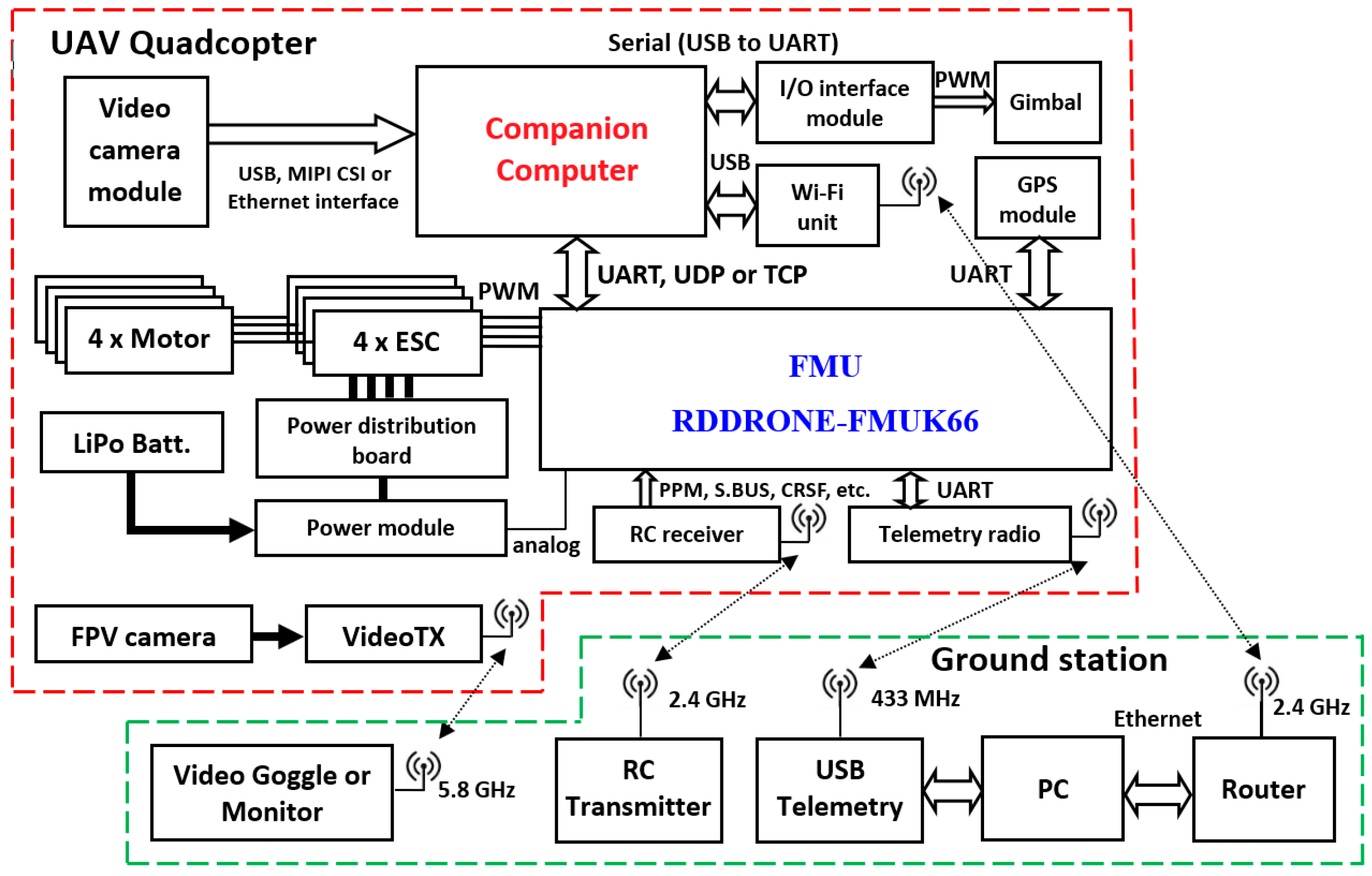
The UAV component of the UAS is based on an NXP HoverGame drone kit. The NXP HoverGame drone kit, known under the commercial name KIT-HGDRONEK66, is composed of all the main mechanical (carbon fiber frame, propellers), electrical (power distribution board (PDB), brushless direct current (BLDC) motors, electronic stability control (ESC) motor controllers), and electronic (the power management module, flight management unit (FMU)—RDDRONE-FMUK66, which also includes different sensors such as a gyroscope, accelerometer, magnetometer, barometer, etc., GPS unit) components needed to build a quadcopter.

The UAV system communicates with the ground control station through four distinct communication links (Figure 1).

The first link is a video link done through a First Person View (FPV) system, allowing a real-time stream of information from the onboard camera. In this mode, the UAV system can be controlled from the pilot’s viewpoint. When the image database was acquired, this system was extensively used to control the quadcopter.

The second link is a radio controller link, which enables a human operator to take control of the UAV by switching from autonomous mode to manual mode. The reverse operation is also possible—by changing the system to offboard mode, the autonomous guidance system located in the companion computer takes control of the UAV. This link is implemented based on a TBS Crossfire 868 MHz long-range system.

The third link is a telemetry link. This is a link based on the Micro Air Vehicle Link (MAVLink) protocol, which enables ground control to communicate with and change the settings of the FMU, configure the flight path, and modify the mission on the fly, among other functions. In this research, the transceivers implementing this link work on 433 MHz. The system uses the 433 MHz wireless band mainly due to the legal constraints imposed by the European Union. In America, this band is on 915 MHz

A fourth link can be utilized and was employed during the system’s development phase. It is a short-range link based on Wi-Fi technology, operating at 2.4 GHz. Through this link, the different images were streamed in real-time using the ZeroMQ (ZMQ) messaging protocol from the companion computer to the ground station. In this mode, the developed algorithm was debugged in real time. ZMQ is a high-throughput, asynchronous, and low-latency protocol.

The NXP HoverGame drone professional kit does not include any software components for flight control or any other components capable of generating intelligent or adaptive behaviors.

The RDDRONE-FMUK66 FMU can run PX4 and ArduPilot autopilots. These two autopilots support a wide range of vehicles, including multi-copters, helicopters, VTOLs [34], fixed-wing aircraft, boats, rovers, and more. In this research, the FMU utilizes the PX4 flight stack, which is built on top of the NuttX operating system (OS).

The guidance of the UAV system is accomplished through a companion computer. Based on the AMD Kria KR260 development board (produced by Advanced Micro Devices, Inc., Santa Clara, CA, USA), the companion computer runs the Ubuntu 22.04 operating system and ROS2 Humble. These two software components can support a wide range of algorithms. The AMD Kria KR260 development board is based on Zynq UltraScale+™ MPSoC, which is composed of the following:

• A 64-bit quad-core Arm Cortex-A53 (up to 1.5 GHz) processor;
• Two ARM Cortex-R5 real-time processors (up to 600 MHz);
• One Mali-400 MP2 GPU;
• One DPUCZDX8G B4096 (4096 MACs per clock cycle) Deep Learning Processor Unit (DPU).

The DPUCZDX8G engine is optimized for the efficient implementation of CNN. In our case, the YOLO DNN was executed on this unit to achieve real-time performance.

The companion computer connects to the FMU by utilizing (1) hardware through a universal asynchronous receiver–transmitter (UART) port; and (2) software based on uXRCE-DDS bridge (between the PX4 autopilot and robot operating system (ROS) 2), supported by the UART port.

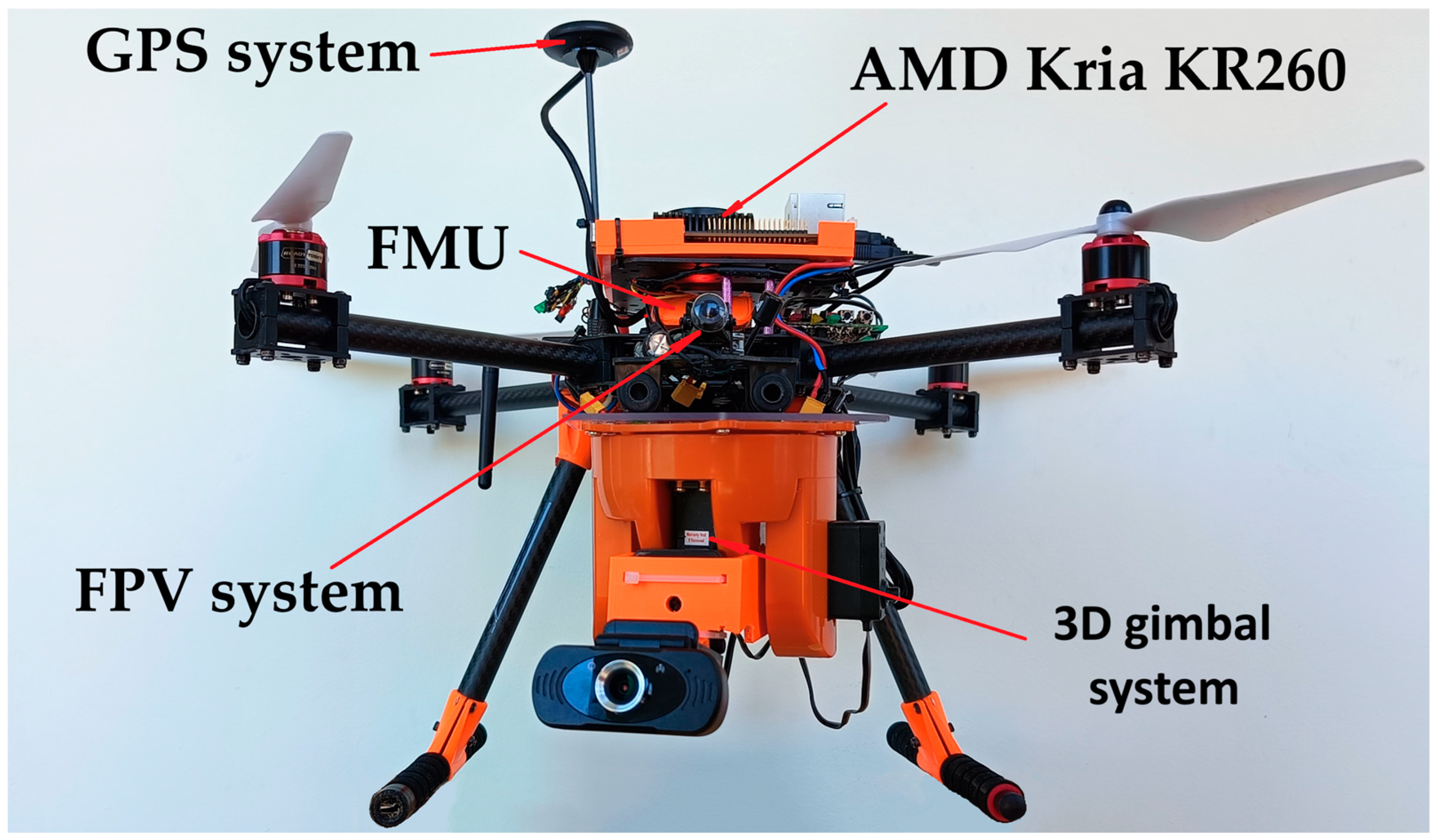
From the presentation of the guidance laws, it is evident that a seeker must identify the target system and establish a lock. Using this system, the LOS can be determined. In our case, the seeker is a 3D gimbal system capable of autonomously pointing a camera at the target, as shown in Figure 2. The 3D gimbal system is controlled by an interface system developed around the MSP430G2553 microcontroller, utilizing two pulse width modulation (PWM) signals to drive the SR431 servomotors. The companion computer controls the 3D gimbal using the RS232 serial protocol. This gimbal system was developed in the frame of this research.

2.2. Image Database

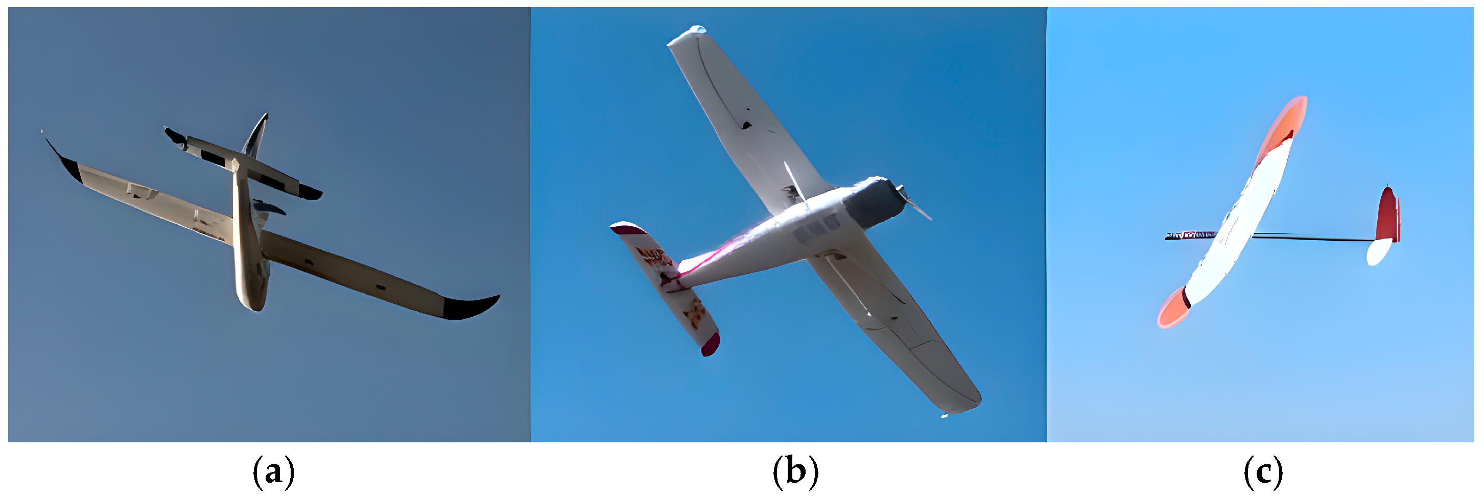
The database was acquired using a GEPRC CineLog35 drone equipped with a GoPro Hero 11 Black to capture the images. The image database used for training and cross-validation consisted of 5605 images, of which 1439 (25.67%) were negative samples. The images were acquired at a resolution of 1920 by 1080 pixels.

The DarkMark framework was used for image annotation. As a direct result, the database contains 2525 annotations with quadcopters and 1943 with planes—in this mode, there are 1.1 marks per image. The recorded quadcopter was the one previously presented in Section 2.1. Three aircraft were used in the image acquisition process: a Cessna model, a Bixler V2, and a glider (Figure 3).

Following the dataset augmentation process, the initial set of 5605 images yielded 19,341 training images and 4835 validation images. Ultimately, 80% of the pictures were used for training, and 20% were reserved for cross-validation of the learning process to prevent overfitting.

Another set of 1524 images were used solely for testing. All accuracy performance analyses presented in the “Performance Analysis” section were conducted on this set. Since both tracking algorithms used in this research require a sequence of images (they need prior detection to predict the information in the next frame), this database includes images from six videos. The images were numbered in ascending order and correspond to the temporal unfolding of the associated videos.

The entire database, comprising images and annotations, occupies 4.85 GB and can be downloaded from the link provided in the Data Availability section.

2.3. DNN Detection Algorithm

2.3.1. YOLO Algorithm

YOLO (You Only Look Once) is a state-of-the-art real-time object detection algorithm able to process images in a single forward pass compared with traditional methods (e.g., R-CNN [25], Faster R-CNN [26], SPP-Net [27], Feature Pyramid Network (FPN) [28]), which use two stages. This approach is significantly faster than traditional methods. The YOLO DNN can simultaneously predict bounding boxes and class probabilities in a single step. Many aspects may be addressed concerning this type of neural network; however, a brief overview of the architectures utilized in this research will be provided: YOLOv3, YOLOv4, and YOLOv7.

The YOLO DNN family was introduced in 2016 when Joseph Redmon and his team proposed this type of DNN [29], YOLOv1, for the first time. This type of DNN transitions to a regression-based approach for bounding boxes, departing from previous approaches based on sliding windows and classification.

YOLOv3 uses multi-scale predictions, allowing it to detect objects of different sizes more effectively [35]. Additionally, the new architecture, Darknet-53, with 53 convolutional layers, improves YOLOv3’s learning capabilities [35].

By utilizing Weighted-Residual-Connections (WRC), Cross-Stage-Partial-connections (CSP), Self-adversarial-training (SAT), Mosaic data augmentation, Cross mini-Batch Normalization (CmBN), Mish-activation functions, DropBlock regularization, and a new CIoU loss function, a new YOLO model was developed: YOLOv4 [36]. The following year, 2021, saw the introduction of two new versions of this algorithm [19]: YOLOv4-tiny, and YOLOv4-large.

YOLOv7 sets a new state-of-the-art, real-time object detection performance, outperforming all previously published YOLO detectors in terms of accuracy. These performances (56.8% on the Microsoft COCO dataset) were achieved by introducing new advanced E-ELAN (Extended Efficient Layer Aggregation Network) and Re-Parameterized Convolution (RepConvN) into the neural network backbone [20].

2.3.2. Evaluation Metrics

The evaluation metrics employed in this research encompass the following: the number of model parameters, frames per second (FPS), precision, recall, specificity, false positive rate, average precision (AP), and mean average precision (mAP).

$$\mathrm{A}\mathrm{c}\mathrm{c}\mathrm{u}\mathrm{r}\mathrm{a}\mathrm{c}\mathrm{y}={\displaystyle \frac{\mathrm{T}\mathrm{P}+\mathrm{T}\mathrm{N}}{\mathrm{T}\mathrm{P}+\mathrm{T}\mathrm{N}+\mathrm{F}\mathrm{P}+\mathrm{F}\mathrm{N}}}$$

(1)

$$\mathrm{A}\mathrm{P}={\int }_0^1\mathrm{P}\mathrm{r}\mathrm{e}\mathrm{c}\mathrm{i}\mathrm{s}\mathrm{i}\mathrm{o}\mathrm{n}\left(\mathrm{R}\mathrm{e}\mathrm{c}\mathrm{a}\mathrm{l}\mathrm{l}\right) \mathrm{d}\left[\mathrm{R}\mathrm{r}\mathrm{c}\mathrm{a}\mathrm{l}\mathrm{l}\right]$$

(2)

$$\mathrm{m}\mathrm{A}\mathrm{P}={\displaystyle \frac{1}{11}}\sum _{\mathrm{i}=1}^{11}{\mathrm{A}\mathrm{P}}_{\mathrm{i}}$$

(3)

$$\mathrm{P}\mathrm{r}\mathrm{e}\mathrm{c}\mathrm{i}\mathrm{s}\mathrm{i}\mathrm{o}\mathrm{n}={\displaystyle \frac{\mathrm{T}\mathrm{P}}{\mathrm{T}\mathrm{P}+\mathrm{F}\mathrm{P}}}$$

(4)

$$\mathrm{R}\mathrm{e}\mathrm{c}\mathrm{a}\mathrm{l}\mathrm{l}={\displaystyle \frac{\mathrm{T}\mathrm{P}}{\mathrm{T}\mathrm{P}+\mathrm{F}\mathrm{N}}}$$

(5)

$$\mathrm{S}\mathrm{p}\mathrm{e}\mathrm{c}\mathrm{i}\mathrm{f}\mathrm{i}\mathrm{c}\mathrm{i}\mathrm{t}\mathrm{y}={\displaystyle \frac{\mathrm{T}\mathrm{N}}{\mathrm{T}\mathrm{N}+\mathrm{F}\mathrm{P}}}$$

(6)

$$\mathrm{F}\mathrm{a}\mathrm{l}\mathrm{s}\mathrm{e} \mathrm{P}\mathrm{o}\mathrm{s}\mathrm{i}\mathrm{t}\mathrm{i}\mathrm{v}\mathrm{e} \mathrm{R}\mathrm{a}\mathrm{t}\mathrm{e}={\displaystyle \frac{\mathrm{F}\mathrm{P}}{\mathrm{F}\mathrm{P}+\mathrm{T}\mathrm{N}}}$$

(7)

In previous equations, TP (True Positive) pertains to objects, such as planes or quadcopters, that are correctly detected by the deep neural network (DNN) and are indeed present. The True Negative (TN) value signifies objects that are neither detected nor present within the frame. FP (False Positive) refers to instances where objects are detected without existing in the image. Conversely, FN (False Negative) indicates cases in which objects are present within the frame but remain undetected by the algorithm. The average precision (AP), as defined in relation (2), is computed as the area beneath the Precision-versus-Recall curve [37]. The mean average precision (mAP) represents the average precision evaluated across eleven equally spaced recall levels [37].

2.4. Tracking Algorithms

Even though YOLO is a state-of-the-art real-time object detection model, it cannot achieve 100% performance. Currently, no detection algorithms reach 100% performance—perhaps such performance can be accomplished only for small problems with few classes and in controlled laboratory environments. In real situations characterized by occlusions, illumination changes, motion blur, scale variation, intra-class variation, viewpoint variation, and background clutter, obtaining 100% detection performance is impossible.

Moreover, after training the DNN and obtaining the best neural model, it must be implemented in the UAV system. At this point, to achieve real-time performance, the DNN model must be executed in a DPU (Deep Learning Processing Unit), NPU (Neural Processing Unit), TPU (Tensor Processing Unit), or GPU (Graphics Processing Unit) system. However, these units have limited processing capacity, so the DNN must be quantized, or a weaker version of the model (nano or tiny, like YOLOv7 tiny) must be utilized. Ultimately, this leads to a drop in the performance of the neural model.

The inability of the YOLO model to achieve 100% detection performance means that, occasionally, it cannot detect the desired target in a frame or a series of frames. However, the flight path control guidance algorithm requires accurate target detection at each control step. To attain this objective, alternative methods must be employed to compensate for the lack of detections in frames or sequences of frames. A potential solution to this issue is to utilize a supplementary tracking algorithm when the YOLO algorithm fails to identify the desired object. To validate the robustness of this approach, the new algorithm used the correlation tracking algorithm (CTA) [38], a Kalman filter, and the YOLO algorithm. Nevertheless, these algorithms also face challenges. For this reason, only the solution integrating all three algorithms has been shown to provide a very high target tracking performance.

2.4.1. Correlation Tracking Algorithm

The correlation tracking algorithm used is based on the implementation of Danelljan et al. [38], and it can accurately track objects in real-time with significant scale variation.

This method extends the Minimum Output Sum of Squared Error (MOSSE) algorithm [39] by learning several separate correlation filters, based on which the target is localized in the new frame. The discriminative correlation filters were extended to multidimensional features by using 1-dimensional filters for scale estimation, 2-dimensional filters for target translation based on Histogram of Oriented Gradients (HOG) features, and 3-dimensional filters for comprehensive scale–space localization of the target. Based on the observations that the scale difference is smaller than a translation of the target between two frames, the algorithm first applies the translation filter, followed by the scale filter. The image representation is based on Principal Component Analysis (PCA)-HOG. The HOG vector is augmented with greyscale image intensity values for robust target representation.

The higher detection accuracy of the CTA is based on HOG features, which significantly improve tracking performance over intensity-based approaches [38]. This algorithm is also computationally efficient due to the decoupling mechanism between translation and scale estimation, which avoids exhaustive scale searches in this mode. Moreover, this CTA approach is modular and can be easily integrated into any tracking framework lacking scale adaptation, making it widely applicable in real-world scenarios.

2.4.2. Kalman Filter

The Kalman Filter estimates the current state based on (a) the estimated state from the previous time step and (b) the current measurement.

This research aims to track a UAV using the center coordinates of the detected bounding box obtained by the YOLO DNN as the measurement. The idea is to use a Kalman filter to continue tracking the UAV even when the YOLO detection fails. Based on the UAV’s estimated position and velocity, the new algorithm can accurately predict its position in the following frame.

The Kalman Filter is composed of two steps.

The first step is the prediction step, in which, by using the process model, the prior state estimate (${\overline{x}}_k$) is predicted. Also, the state estimate error covariance matrix (${\overline{P}}_k$) is computed. Based on ${\overline{P}}_K$, the Kalman Filter estimates how much to trust the current values of the predicted state [1].

$${\overline{x}}_k=F·x_{k-1}+B·u_k+w_k$$

(8)

$${\overline{P}}_k=F·P_{k-1}·F^T+Q_k$$

(9)

The state vector is the position and velocity of the UAV on the x and y directions (${\overline{x}}_k={\left[x_k,y_k,{\dot{x}}_k,{\dot{y}}_k\right]}^T)$. The state transition matrix model was obtained from second-order equations of motion, and it has the following form ($∆t$ is the time between two frames) [1]:

$$F=\left[\begin{array}{ccc}1& ∆t& \begin{array}{cc}0& 0\end{array}\\ 0& 1& \begin{array}{cc}0& 0\end{array}\\ \begin{array}{c}0\\ 0\end{array}& \begin{array}{c}0\\ 0\end{array}& \begin{array}{cc}\begin{array}{c}1\\ 0\end{array}& \begin{array}{c}∆t\\ 1\end{array}\end{array}\end{array}\right]$$

(10)

B is the control input model matrix, which in our case is the zero matrix, and $w_k$ is the predicted process noise, assumed to be a zero-mean multivariate normal distribution with covariance matrix Q:

$$w_k=N\left(0,Q_k\right)$$

(11)

The second step is the update step, where the prior prediction is combined with the measurement (based on Kalman gain) to obtain the state estimation ($x_k$)—the output result of the Kalman Filter.

$$z_k={H·x}_k+v_k$$

(12)

$$K_k={\displaystyle \frac{{\overline{P}}_k·H^T}{{H·\overline{P}}_k·H^T+R_k}}$$

(13)

$$x_k={\overline{x}}_k+K_k·\left(z_k-H·{\overline{x}}_k\right)$$

(14)

$$P_k=\left(I-K_k·H\right)·{\overline{P}}_k$$

(15)

In relation (12), $z_k$ is a measurement at the k moment of the true state $x_k$, and v_k is the measurement noise, assumed to be also a zero-mean Gaussian white noise with covariance matrix R.

$$v_k=N\left(0,R_k\right)$$

(16)

The H matrix is the observation model which maps the true state space into the measurement space, and in the case of our problem, has the following form:

$$H=\left[\begin{array}{ccc}1& 0& \begin{array}{cc}0& 0\end{array}\\ 0& 0& \begin{array}{cc}1& 0\end{array}\end{array}\right]$$

(17)

The Kalman gain ($K_k$), see relation (13), is a measurement of the information existing in the sensors. The Kalman gain and the error in the sensors are inversely correlated—the higher the error in the measurement, the smaller the Kalman gain will be and vice versa. $P_k$is the new error covariance matrix after the measurement is embedded into the state estimation.

3. Results

3.1. The UAS System

The proposed UAS development platform is based on a highly versatile approach at all levels, including hardware and software, as well as at the levels of the UAV and the ground station.

For example, the companion computer can be easily replaced with another development system based on a different processor or another DNN processing core. In a preceding application, the i.MX 8M Plus development board was employed [40,41]. In this board, the DNN inference process is performed on an NPU. To port the code from the current implementation to the i.MX 8M Plus, the only changes that need to be made are those related to loading the neural model onto the NPU. Changing the communication channel to Ethernet (between the FMU and companion computer) requires only two simple configurations. Furthermore, it is possible to utilize a protocol that is not supported by PX4, such as I2C [42]. In this case, it becomes necessary to develop and incorporate the corresponding code within the PX4 autopilot system.

Similarly, various types of radio-controlled (RC) systems operating on different protocols can be integrated into this UAV. Many receivers based on different protocols (PPM, S.BUS, CRSF, GHST, etc.) can be easily interfaced with the PX4 autopilot [40,41,42,43].

The versatility of the PX4 autopilot manifests itself on multiple levels. One of the advantages of this autopilot is its ability to integrate with the MATLAB Simulink package (version R2024b) through the UAV Toolbox Support Package [43,44]. Furthermore, simulators such as Gazebo or JmavSim are used to model realistic flight dynamics using the Software-in-the-Loop (SITL) approach [34,45]. Finally, the Hardware-in-the-Loop (HIL) simulation mode may be referenced, in which the PX4 firmware operates on an actual hardware Flight Management Unit (FMU) and is integrated with a Gazebo or JmavSim simulator [44].

One of the key features of this UAS ecosystem is its open-source software and hardware architecture based on Apache NuttX RTOS, PX4 open-source flight controller, MAVLink protocol, Ubuntu OS, ROS2 middleware, Kria Robotics Stack, QgroundControl, ZeroMQ library, SiK Telemetry Radio platform, and Pixhawk (hardware standard for FMU).

3.2. The Tracking Algorithm

The new proposed tracking algorithm is based on a YOLO DNN model. When YOLO cannot detect UAVs, the Correlation Tracking Algorithm (CTA) takes over the operation, based on YOLO’s last correct detection, but only for up to nine consecutive frames. If the YOLO algorithm fails to detect the object (the UAV system) for more than nine consecutive frames, the Kalman filter will initiate drone tracking operation on all subsequent frames. On all the frames where YOLO and CTA had detections, the Kalman filter runs both stages: prediction, and update. In all other frames, only the prediction step is active. The complete data processing flow within the system (on DPU and CPU) is depicted in Figure 4.

This approach resulted from the following observations and analyses:

• Through the integration of YOLO and CTA, it was observed that the CTA algorithm is capable of accurately tracking the UAV system (including drones or airplanes) for a minimum of 10 consecutive frames and a maximum of 17 frames.
• A comparative analysis of the results obtained by integrating YOLO and CTA, as opposed to YOLO and Kalman, utilizing a substantial dataset of recordings, indicates comparable performances, as demonstrated in the following table. The execution time for the CTA is approximately 61 milliseconds, resulting in a performance reduction of 1.5 frames per second when executed independently. Conversely, the Kalman filter operates with a quicker execution time of 5 milliseconds. Accordingly, it is recommended to execute YOLO and CTA concurrently, followed by the sequential execution of the Kalman filter, rather than executing YOLO and the Kalman filter concurrently, followed by the execution of the CTA algorithm.

The lower section of Figure 4 presents the timing diagram for each respective algorithm. The YOLO algorithm has an execution time of 148 milliseconds. When YOLO successfully makes a correct detection, as indicated by the YOLO detection(s) in Figure 4, the control algorithm will rely exclusively on the information obtained from this detection. In the event of a failure within the YOLO detection system, data retrieved from the CTA or the Kalman filter will be utilized. Nevertheless, the YOLO detection system continuously functions in the background, actively searching for new objects to detect. Once a correct detection occurs, after a missed detection or a series of unsuccessful detections by the YOLO algorithm, a switch will be executed from either the CTA or the Kalman filter to the YOLO algorithm.

3.2.1. Training the YOLO Models

First, the YOLO neural network must be selected and trained to implement all the abovementioned steps. The contenders for the chosen algorithm are the three neural models, YOLOv3, YOLOv4, and YOLOv7, all of which have tiny versions.

All these neural network models are part of the Darknet framework.

Table 1. A short presentation of the YOLO models used in this research.

YOLO Version	Layers	Number of Parameters		Input Image Size
		Trainable	Non-Trainable
YOLOv3 tiny	44	8,669,876	6368	640 × 480
YOLOv4 tiny	76	5,874,116	6208	640 × 480
YOLOv7 tiny	198	6,016,735	14,784	640 × 480

presents a brief description of their complexity.

Before the training, the images were resized to match the allowed image input size of 640 × 480 pixels. The standard YOLO network image input size is 416 × 416 pixels. By adjusting the input image sizes, the YOLO network modified the input layer dimensions; as a result, the optimal YOLO anchors were recalculated.

The YOLO models were trained on a personal computer equipped with a GeForce RTX 4080 Super GPU, as well as on a more powerful machine featuring four NVIDIA Tesla A100 Ampere GPUs, which significantly accelerated the training process.

Each version of the YOLO DNN was trained multiple times (at least 20 different training instances with various parameters), and the best results are presented in

Table 2. The obtained performances for each version of the algorithm.

YOLO Version	Class	Average Precision	Accuracy	Error Rate	Precision	Recall	Specificity	False Positive Rate
YOLOv3 tiny	Quadcopter	96.237	0.9505	0.0495	0.9527	0.9382	0.9608	0.0392
	Plane	87.855	0.9219	0.0781	0.8912	0.8433	0.9557	0.0443
YOLOv4 tiny	Quadcopter	97.023	0.9603	0.0397	0.9400	0.9547	0.9637	0.0363
	Plane	90.888	0.9434	0.0566	0.8508	0.9016	0.9552	0.0448
YOLOv7 tiny	Quadcopter	95.088	0.9460	0.0540	0.9040	0.9269	0.9548	0.0452
	Plane	81.022	0.9324	0.0676	0.8523	0.7484	0.9720	0.0280

.

The results shown in Table 2 are those obtained from the Darknet framework at the end of the training process. Essentially, each new version of the YOLO algorithm yields improved performance (e.g., mAP) over its predecessor. Based on Table 2, it is observed that YOLOv4 demonstrates an enhancement in detection performance relative to YOLOv3, whereas YOLOv7 exhibits the lowest performance among the three neural networks.

The global learning curves from Figure 5 are for both classes for the YOLOv3 tiny neural model. The red line represents the precision achieved by the deep neural network on the validation set, while the blue line depicts the loss of the neural network. The framework automatically saves the trained weights every 1000 iterations, as well as the best weights obtained throughout the entire training process.

The following graphs (Figure 6) present the learning curves for training the YOLOv3-tiny neural model for each class. On the left, the results for the quadcopter class are presented, whereas the results for the plane class are displayed on the right. The imbalance in data for the plane class is evident in the lower performance observed in this class, as shown in the right graph. In all the graphs, the cross-validation loss decreases with each epoch, accompanied by an increase in mean average precision, which saturates at maximum values after epoch 14,400 (for the plane class) and after 12,800 for the quadcopter class. The learning process was smooth for the quadcopter class but somewhat volatile for the plane class, with a spike occurring around epoch 8000. This fluctuation is likely attributed to a slightly higher learning rate for the plane class. This learning rate was determined after numerous attempts and proved to be the most effective for achieving the highest possible accuracy.

At the end of the training of the YOLO neural models, two components were obtained: (a) a yolo.cfg file, containing the architecture of the DNN; and (b) a yolo.weights file, which is embedded inside all the resulting weights.

3.2.2. Deploying YOLO on the Real System

Deploying a YOLO model on the AMD Kria KR260 development board is not a straightforward operation. The YOLO neural model (comprising the yolo.cfg and the yolo.weights files) must be converted to a specific yolo.xmodel file that is compatible with the DPU located inside the development board. The Zynq UltraScale+ MPSoC chip (found on the Kria KR260 Robotics Starter Kit) incorporates the DPUCZDX8G DPU. Although the DPUCZDX8G DPU is a highly powerful chip, capable of running a DNN structure with 198 layers (Table 1), it also has several limitations. These limitations come from the lack of support for various neural layer types and the limited flexibility in utilizing different building blocks within DNN, such as restricted kernel sizes, limited stride steps, or a limited range of activation functions.

As will be immediately evident, one of these limitations is the inability to execute any type of neural layer present in a DNN network.

In the first step, the YOLO model was converted to a Keras HDF5 model data format. All the original YOLO models used an internal 32-bit floating-point representation. Next, using the Model Inspector tool in the second step, the Keras model was inspected to determine its compatibility with the specific AMD DPU architecture. If it was compatible, it could go on to the third step, where the model was quantized to an 8-bit fixed-point format. In the final step, based on the 8-bit representation of the DNN, the model was compiled to generate a microcode file (.xmodel) that could be executed within the DPU. The anchors were recomputed as a direct result of this conversion process. The “Supplementary Materials” section presents links to materials that describe all these steps in detail and all the source code necessary for the conversion process.

YOLOv4 tiny and YOLOv7 tiny neural structures encountered problems during the conversion process. For the YOLOv7 tiny neural model, the “Swish” nonlinearity layers were not supported by the DPU, while for YOLOv4 tiny, the “Mish” nonlinearity layers faced the same issue. Consequently, both neural networks were structurally modified by substituting the existing layers with “LeakyReLU” nonlinearities. Of course, utilizing the “Swish” and “Mish” activation functions allows the YOLO models to achieve the best results, with the highest mAP and lowest validation losses. However, the only way to obtain a model compatible with the DPU was to use a “LeakyReLU” nonlinearity. Moreover, in the context of the YOLOv4 neural network model, “Lambda” neural layers were also unsupported. These layers are designed to model long-range dependencies within the data, which conventional convolutional layers may struggle to capture. This characteristic makes Lambda layers an indispensable component within the YOLOv4 architecture. Several attempts to replace them proved unsuccessful, resulting in a decrease in accuracy of more than 14%. Furthermore, efforts to execute these three Lambda neural layers on the CPU while running the remainder of the network on the DPU caused unacceptable delays in data processing. Consequently, it was decided to terminate the further utilization of the YOLOv4 neural network model.

By quantizing the neural models and substituting some neural layers in the original architecture, a slight degradation in the detection performance of both YOLOv3 and YOLOv7 neural models was observed.

From

Table 3. A presentation of the temporal performance achieved by the YOLO algorithms used in this research.

YOLO Version	DPU Processing Time [s]	DPU Processing and Data Transfer Time [s]	YOLO data Decoding Time [s]	Global Performances [FPS]
YOLOv3 tiny	0.02496	0.13925	0.0079	5.8
YOLOv7 tiny	0.03050	0.15703	0.2135	2.5

, the performances of the neural models YOLOv3 tiny and YOLOv7 tiny are somewhat similar (24.9 ms versus 30.5 ms), with a slight advantage in favor of the YOLOv3 tiny model. Unfortunately, decoding the outputs of the neural model takes a long time in the YOLOv7 tiny model due to the suppression of a large number of boxes detected—Non-Max Suppression (NMS). This led us to use the YOLOv3 tiny neural model further in the implementation of the final algorithm.

Additionally, the performance of the YOLOv3 and YOLOv7 neural models (the full versions) was tested; however, they did not meet the real-time requirements of the UAV system. For example, YOLOv3 achieved 2.9 FPS, while YOLOv7 reached only 0.93 FPS.

Another identified issue was the one illustrated in Figure 7. When comparing the ground truth bounding boxes (those annotated by the human subject), which are shown in Figure 7 in green (the smaller ones) with the bounding boxes detected by the YOLO algorithm, depicted in Figure 7 in red (the larger ones), it was found that the detected boxes are larger than the ground truth bounding boxes. This implies that a maximum value of 0.46 and an average value of 0.21 were attained in the computation of the Intersection over Union (IoU).

From a practical standpoint, this is not an issue, considering that only the center of the detected bounding box is crucial in a UAV system’s guidance algorithm. However, when calculating accuracy performance (such as mAP), it was required to select a lower value for the IoU threshold.

3.2.3. Performance Analysis

As previously presented, an algorithm for guiding a UAV relative to the position of another UAV system requires the coordinates of the latter UAV to make all the necessary trajectory corrections. These coordinates delineate the centers of the detected bounding boxes. Consequently, in addition to employing traditional metrics to evaluate detections, such as mAP, precision, or recall, an additional parameter has also been introduced. This parameter represents the distance between the centers of the ground truth bounding boxes and the center of the detected bounding boxes. This parameter defines the positioning error of the center detection compared to the UAV system’s actual position. Higher accuracy detection requires a value as small as possible, approaching zero. However, this newly introduced parameter has a problem: What happens when an existing UAV system is not detected? It is evident that, under these circumstances, calculating such a distance is unfeasible; however, the implementation of a penalty factor is necessary. In the most adverse scenario, the UAV system is situated in one corner of the image, while the detection occurs in the diagonally opposite corner. The distance between the two bounding boxes is slightly smaller than the diagonal of the image. Therefore, in the case of no detection, an error distance equal to the diagonal of the image was chosen.

The YOLO neural network returns (a) several bounding boxes, (b) the class of each element placed inside a bounding box, and (c) the class probability of detection. However, the CTA and Kalman filters do not detect new objects (e.g., they do not return new bounding boxes with new dimensions and new associated probabilities); both methods cannot run alone, they need a starting point, so they rely on previous information to estimate the new position of the tracked object. Consequently, for the CTA and Kalman algorithms, a bounding box was utilized, configured with the most recent detected dimensions supplied by the YOLO neural network. The detection probability of 0.7 was used when YOLO had no detections. This value represents the approximate average probability of detections for quadcopters as output by the YOLO deep neural network.

The YOLO neural network was always executed on the DPU unit. The CTA operated in parallel, with the code being executed on one of the ARM Cortex-A53 processor cores. Furthermore, the execution time of the CTA, which is 61 ms, consistently remained shorter than that of the YOLO DNN on the DPU. The Kalman Filter was executed subsequently, following the YOLO and CTA executions.

Table 4. Performance of different algorithms used in the UAV tracking process for the entire test set.

	YOLO	YOLO and CTA	YOLO and Kalman Filter	YOLO, CTA, and Kalman Filter
mAP	68.97%	74.15%	74.53%	83.73%
Precision [%]	93.87 ± 1.2%	88.36 ± 1.61%	88.82 ± 1.58%	90.26 ± 1.49%
Recall [%]	75.33 ± 2.16%	88.12 ± 1.61%	88.58 ± 1.59%	90.03 ± 1.5%
GT Count	1524	1524	1524	1524
Det. Count	1223	1524	1524	1524
mean Dist.	440.0	22.7	18.3	17.9

shows the performances achieved by the algorithm proposed in this paper (last column), as well as the individual contributions of each component to the overall system performance. It also includes the YOLO model compiled for the DPU architecture (second column), the performance without the Kalman filter (third column), and the performance without the CTA in the fourth column.

Table 4 also clearly and unequivocally demonstrates that the lowest performance metrics, observed from all perspectives, are exclusively attained when the YOLO algorithm is applied alone. The application of either the CTA or Kalman algorithms in conjunction with YOLO yields performance enhancements; however, these improvements are not as substantial as those achieved when utilizing a combination of all three algorithms.

The results presented in Table 4 are derived from the evaluation procedure described in [37] for the Pascal Visual Object Classes (VOC) Challenge.

In Table 4, for human readability, the mAP is shown as a percentage even though the underlying metric remains a number between 0 and 1. To quantify the uncertainty in precision and recall estimates, the confidence intervals are provided in Table 4. With the test set of 1524 images, there is a 95% chance that the interval from 88.75% to 91.75% contains the true model precision—the precision for the YOLO, CTA, and Kalman Filter algorithms. Similarly, the model proposed in this paper achieved a recall of 90.03% ± 1.5% at a 95% confidence level.

According to Table 4, the proposed algorithm shows the smallest average distance between the centers of the ground truth bounding boxes and detected bounding boxes (mean Dist.) as 17.9, which is a significant improvement compared to the YOLO algorithm (440).

Because complex situations where all three algorithms (YOLO, CTA, and Kalman Filter) must work together to maintain persistent and steady detection are infrequent, their performance diminishes in many relatively simple scenarios, especially when detections are briefly lost (for just 1, 2, 3, or 4 frames), or when there are no errors in detection. Below, we present a performance analysis for a complex case where the YOLO algorithm fails to detect a drone in 36 successive frames, from t1 to t2, as shown in Figure 8.

The trajectory from Figure 8 is only the most challenging part of the trajectories analyzed in

Table 5. Performance of different algorithms used in the UAV tracking process.

YOLO Version	YOLO	YOLO and CTA	YOLO and Kalman Filter	YOLO, CTA, and Kalman Filter
mAP	63.64%	72.11%	71.35%	90.48%
Precision [%]	100 ± 0%	85.23 ± 5.7%	83.89 ± 5.9%	99.33 ± 1.31%
Recall [%]	66.44 ± 7.58%	85.23 ± 5.7%	83.89 ± 5.9%	99.33 ± 1.31%
GT Count	149	149	149	149
Det. Count	99	149	149	149
mean Dist.	743.35	51.72	35.9	11.4

. In this table, the YOLO network fails to detect the UAV in 50 of the 149 video sequence frames, which matches the ground truth count (GT Count), due to the presence of a single UAV in each frame.

The results presented in Table 5 are based on a data segment from the testing database, where achieving UAV system detections using the YOLO DNN is challenging. Only 149 out of the 1524 frames in the test set were utilized.

The YOLO algorithm’s inability to detect the UAV system over 36 consecutive frames arises from a combination of factors: (a) a complex background spanning four different areas (sky, hill, houses, and field), (b) variability in the size of the UAV system as it approaches the recording point, (c) fluctuations in the UAV’s speed and trajectory, and (d) performance losses due to DNN conversion to the DPU.

Table 5 indicates that the optimal accuracy of object detection, as measured by mean average precision (mAP), attains its highest value when employing a combination of all three algorithms: YOLO, CTA, and Kalman Filter. Conversely, the lowest value is observed when utilizing solely the YOLO neural network. This observation reinforces the notion that the YOLO neural network is insufficient on its own for tracking an object through its detections across multiple frames. The accuracy of detections improved when the YOLO algorithm was enhanced with CTA or Kalman Filter. Furthermore, it is observed that the mean distance between the actual position of the Unmanned Aerial Vehicle (UAV) and its detection is minimal when utilizing the newly proposed global algorithm in this paper, which is based on the synergistic operation of the three individual algorithms.

Ultimately, these performances, presented in Table 5, are generated by the accurate detection and tracking capabilities of the various algorithms employed in this research.

As shown in Table 5, the higher value of 90.48% for mAP indicates a significant improvement over the 63.64% achieved by the YOLO DNN. Additionally, precision and recall provide an accurate estimate of 99.33% ± 1.31%. To observe the performance of various algorithms and their combinations in real-time, please refer to the video linked in the “Supplementary Materials” section, specifically item two. As demonstrated, the UAV system was successfully detected in all frames. All data presented in Table 5 are based on the results from this video (https://youtu.be/MuwVoTvQBYc, accessed on 13 May 2025).

During periods of maximum system load, when the algorithm functioned concurrently on the CPU and DPU, the current consumption of the Kria KR260 development system was measured at 840 mA, as opposed to 725 mA before its deployment. When comparing these values with the consumption of the hovering UAV system, which is 23 A, or with the maximum consumption of the drone at 138 A (at full throttle), it is observed that the consumption of the development system is merely 0.58% to 3.5% of the total consumption of the UAV system.

Regarding the computational burden, the peak system load is recorded at 2.88 (out of a maximum of 4, corresponding to the four CPU cores), with an average load of 2.43 out of 4. When the algorithm is inactive, the Ubuntu 22.04.5 LTS (long-term support) operating system maintains an average load of 0.09 out of 4.

The thermal cooling solution for the Kria KR260 is an active one, comprising a heatsink and a fan. The system was developed by AMD for a total maximum thermal power of 15 W. After one hour of active operation of the tracking algorithm, the heatsink reached a maximum temperature of 33 °C. The component with the highest temperature on the board was a voltage stabilizer, which reached 42.1 °C, as shown in Figure 9. At the time of this measurement, the ambient temperature was 21 °C.

4. Discussion

Numerous previous studies have aimed to enhance the detection accuracy of systems implemented with either classical or deep learning algorithms. Considering that this research is based on a deep neural network (DNN) algorithm, the analysis will, therefore, be conducted exclusively on this category of detection system. Each of the previous works aims to enhance detection accuracy or optimize a specific aspect of deep neural networks (DNNs).

For example, in the first approach, accuracy is increased by employing a new type of DNN, such as the CFAMet neural network [46], or by using a novel perceptual GAN model [47]. In a second approach, different types of improvements are made to (a) the YOLOv5 algorithm, resulting in two new algorithms, YOLO-LSM [31] and UA-YOLOv5s [48]; (b) YOLOv7, resulting in YOLO-DCTI [32]; and (c) YOLOv8, resulting in SP-YOLOv8s [49]. However, these algorithms also have disadvantages, the most significant being the increase in computational load that accompanies the improvement in algorithm accuracy, as seen with the SP-YOLOv8s [49] neural network.

No matter how robust a single detection algorithm is, it will be impossible for it to track a target in all the frames it acquires. There will inevitably be frames in which no detections occur or false-positive detections occur. Furthermore, when executing this algorithm on the UAV, due to its constrained computational resources, there will be supplementary performance degradation (attributable to model quantization, architectural modifications, or the utilization of a less complex variant of the DNN), which may result in the absence of detections in additional frames.

The algorithm proposed in this paper aims to address these issues. From Table 4 and Table 5, in the case of the detection algorithm presented in this paper, the number of ground truth bounded boxes is equal to the number of detected bounded boxes with the minimal distance between their centers. Therefore, there are no frames with missed detections.

Analyzing the data from Table 4 and Table 5, it can be observed that the CTA and Kalman Filter algorithms, used individually with YOLO or in combination, provide a performance boost over the YOLO detection algorithm. Moreover, our YOLO detection algorithm can be replaced with any of the previous algorithms [31,32,46,47,48,49]. Therefore, this new approach will undoubtedly enhance the performance of any initial algorithm employed in detection.

Among the similar works on this topic, Akyon et al. [33] developed a detection algorithm that closely aligns with the approach presented in this paper. This algorithm represents the winning solution in the Drone vs. Bird Challenge, organized as part of the 17th IEEE International Conference on Advanced Video and Signal-Based Surveillance. As in our case, the data are augmented. The detection algorithm, the first step, is based on a YOLOv5 deep neural network (DNN), followed by a Kalman filter to enhance detection performance [33]—the second step. At this point, a notable difference emerges compared to the algorithm presented in this paper; in [33], the Kalman filter is used solely to eliminate false positive detections. In the third step, a tracking boosting method is used to increase the algorithm’s confidence. The results obtained are presented in

Table 6. Comparative performance analysis of our algorithm versus the [33] algorithm based on the mAP parameter—comparison of absolute values.

The Algorithm Proposed in [33]		Short Section of the Database, Table 5	Entire Database, Table 4	Proposed Algorithm
YOLOv5	0.781	0.6364	0.6897	YOLOv3 tiny
YOLOv5 + Tracker	0.788	0.7211	0.7453	YOLOv3 tiny + CTA
YOLOv5 + Tracker + Track Boosting	0.794	0.9048	0.8373	YOLOv3 tiny + CTA + Kalman Filter

.

On the right side of Table 6, the performances achieved by the proposed algorithm for both the entire test database and a single section are also shown. A direct comparison of the two algorithms based solely on the absolute mAP values is, therefore, not possible. Nevertheless, even within this context, the overall performance indicates the superiority of the algorithm proposed in this paper, with an mAP of 0.837 (or 0.905) in comparison to 0.794.

A comparison of absolute performance is inappropriate because, as referenced in [33], a more recent iteration of the YOLO algorithm is utilized, which operates on a personal computer; thus, there are no constraints on real-time execution. Furthermore, YOLOv5 was not subjected to quantification; its architecture remained unaltered—no layers were diminished—and therefore employed the architecturally optimal configuration. Additionally, a reduced version of this algorithm was not utilized. Nonetheless, given the similarity between both algorithms, which are based on a combination of three distinct algorithms,

Table 7. Relative comparison of the performances of the proposed algorithm versus the [33] algorithm, using the YOLO detection algorithm as a reference base.

The Algorithm Proposed in [33]		Short Section of the Database	Entire Database	Proposed Algorithm
YOLOv5	1	1	1	YOLOv3 tiny
(YOLOv5) + Tracker	1.0089	1.1331	1.0806	(YOLOv3 tiny) + CTA
(YOLOv5 + Tracker) + Track Boosting	1.0076	1.2547	1.1234	(YOLOv3 tiny + CTA) + Kalman Filter
Overall improvement	1.0166	1.4217	1.2140	Overall improvement

illustrates the performance enhancement achieved by integrating the new detection capabilities with the previous results, using the YOLO algorithm as the reference point.

From Table 7, the overall performance improvement achieved by the combination used in this paper (CTA and Kalman Filter) is superior (around 1.2 up to 1.4) to that of the combination used in [33], which yields an mAP increase of only 1.0166.

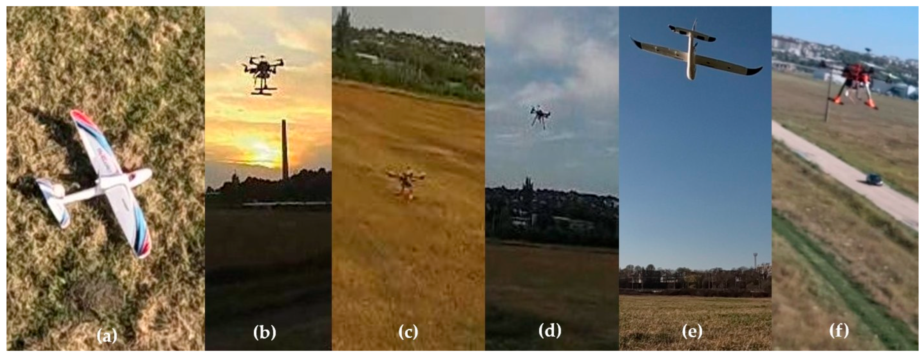
The algorithm developed and presented in this paper shares the same deficiencies as all comparable algorithms [14,15,16,18,19,20,21,22,23,24,25,26,27,28,29,30,31,32]. In a real-world context, detection accuracy is influenced by factors such as lighting conditions, dynamic shadows, contrast levels, viewing angles, or scale variations. To mitigate these challenges, two distinct methodologies were employed. The first approach involved compiling an extensive and diverse training dataset, as illustrated in Figure 10. The images were collected under various weather conditions: on sunny days (Figure 10a), at dusk (Figure 10b), during cloudy weather (Figure 10d), and under a “gray” sky (Figure 10c,e). To address scale discrepancies, images were captured from varying distances relative to the target, as exemplified in Figure 10c,d,f. Additionally, to improve adaptability to different perspectives, images of the target were acquired from multiple viewpoints, including from above (Figure 10a), below (Figure 10e), and from various side angles (Figure 10b–d,f).

The second approach was predicated on image augmentation. Through the augmentation process, starting from an initial set of 5605 images, a total of 19,341 training images were generated. The employed data augmentation techniques introduced new variations within the training dataset, such as random rotations, flips, cropping, and alterations in image color properties, including brightness, contrast, saturation, and hue. As a direct consequence, the deep learning model enhanced its robustness and its capacity for generalization.

The analysis of the algorithm’s detection capacity with altitude reveals that the background and proximity to the detected object predominantly influence it. Consequently, altitude is not an essential factor; an object situated at either low or high altitude against the sky is detected more readily than an object at the same altitude with a complex background, such as houses, forests, or fields. This observation is substantiated by both Figure 8 and the video provided in the “Supplementary Materials” section.

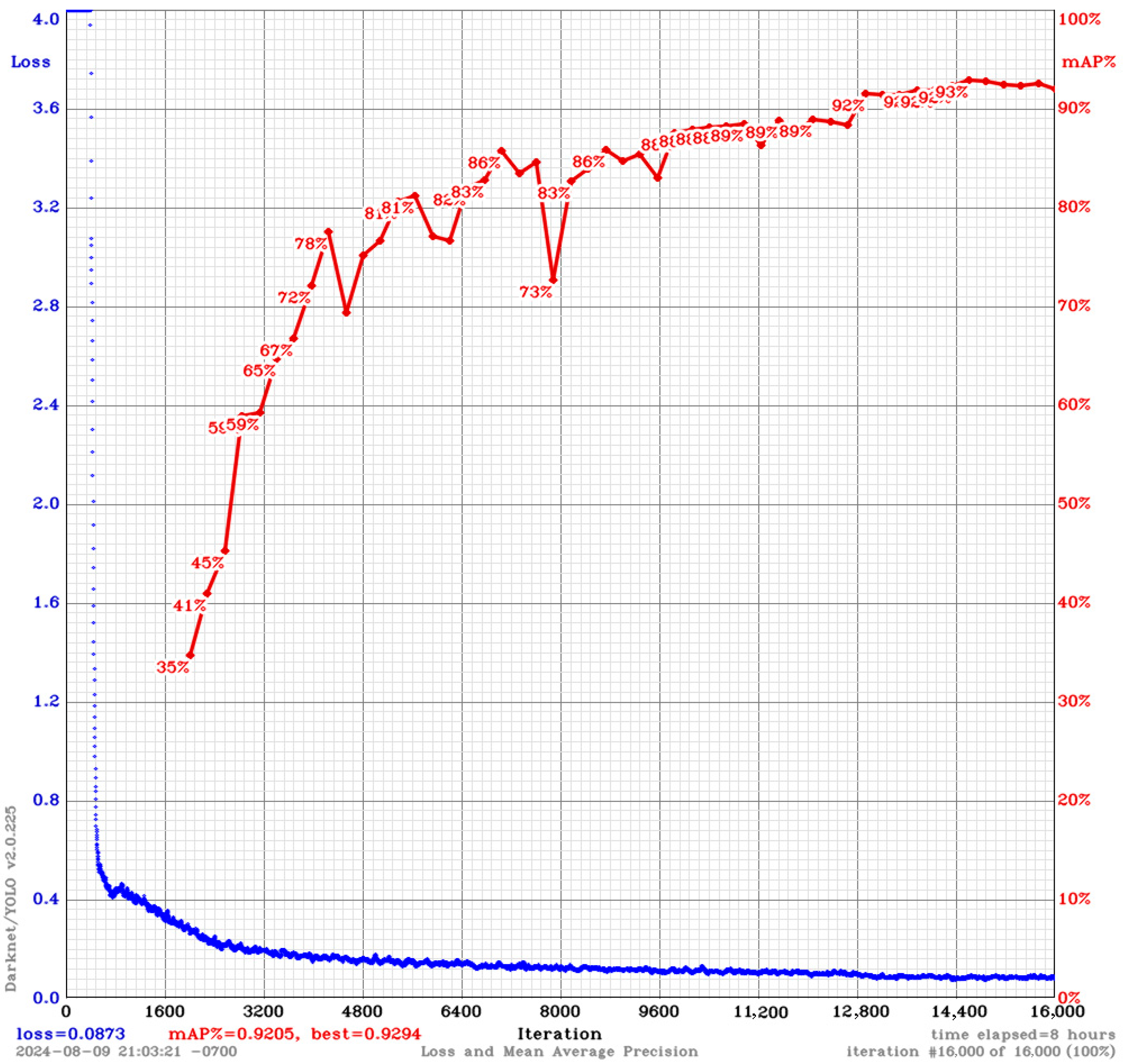
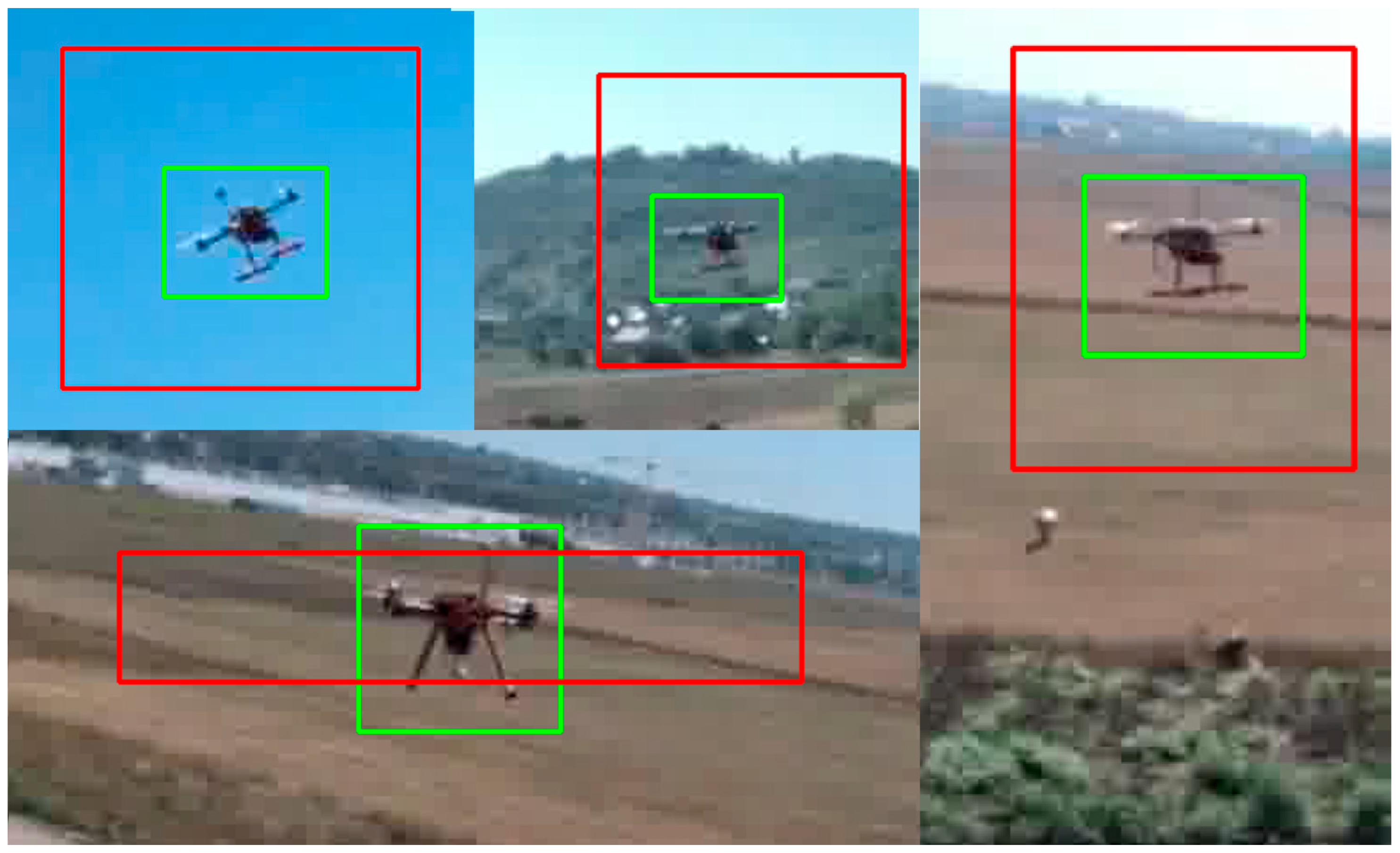
Based on the operation of the novel algorithm and the results presented in Table 4 and Table 5, it is evident that it is highly effective. For instance, analysis of the results in Table 5 reveals a mean average precision (mAP) of 90.48%, with precision and recall values of 99.33% ± 1.31%. Nonetheless, these parameters (mAP, precision, and recall) also encompass information regarding the extent of overlap between the object’s bounding box annotation and the detection box generated by the algorithm, as demonstrated in Figure 7. All results in Table 5 were derived exclusively from the video included in the “Supplementary Materials” section. In this video, no frame exhibits either a lack of high-quality detection or false positives. The reason for mAP not reaching 100% or a value very close to it is that the detected boxes tend to be larger than the ground truth bounding boxes, as illustrated in Figure 7. Despite these high detection performance metrics, it remains plausible that, in the final stage, the Kalman algorithm may produce an erroneous output, or the YOLO may have a false positive detection. In such cases, these issues were partially mitigated through the implementation of “if” decision structures. For example, when a new detection is significantly distant from the previous one, the control algorithm relies on the prior detection to guide the drone. Moreover, in the absence of any detection, such as during the initial activation of the algorithm, the drone’s control is transferred to the operator. Alternatively, the drone ascends to a predetermined altitude, where a slow rotation around the vertical axis perpendicular to the ground begins until the first detection is achieved.

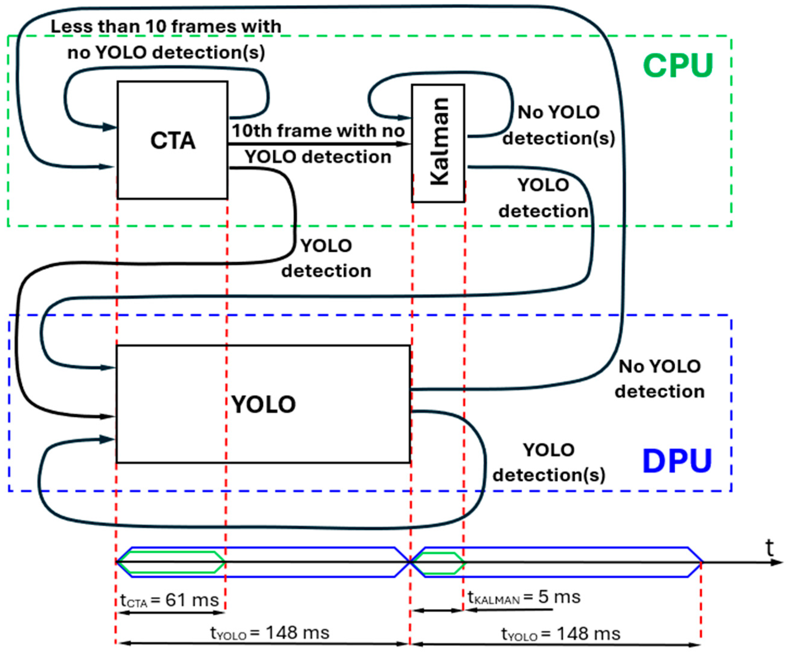
UAV control is accomplished via a velocity-based methodology utilizing an application developed and operated within the ROS2 environment. From this perspective, the application determines a specific set point, which in this instance, is a designated velocity. The internal PX4 control loops perpetually maintain the stability of the UAV system’s dynamics by utilizing this set point for subsequent updates. In offboard mode—when the vehicle adheres to setpoints supplied by an external source outside the flight stack—the companion computer is required to stream setpoints at a rate exceeding 2 Hz; failure to do so will result in the vehicle exiting offboard mode. In the worst case (with YOLOv3 detections), the developed algorithm produces setpoints at a rate of 5.8 Hz. This rate can increase to 15 Hz with CTA detections or 140 Hz with Kalman filter detections, see Figure 4. During all field tests, both the tracking UAV system and target UAV were of the same types described in Section 2.1 of this paper. This UAV system, based on the HoverGames drone, can attain a maximum speed of 68 km/h, approximately equivalent to 19 m/s. At their maximum velocity, the UAV systems operate, in the worst-case scenario, with a setpoint supplied 5.8 times per second, which corresponds to a correction for every 3.3 m of the drone’s travel. For these two deployed UAVs, this update frequency proved to be adequate, as the drone’s trajectory remained smooth, primarily due to the interplay between the current trajectory and the preceding one, integrated through the drone’s inertia. Clearly, as the speed of the tracking system increases, the 5.8 Hz trajectory modification rate of the tracking system can become insufficient in such scenarios. Therefore, additional optimizations of the detection system must be implemented. Alternatively, the operational frequency of the DPU system must be increased, or an alternative DNN system should be considered for replacement.

Through the utilization of the communication interface between the companion computer and the FMU, GPS coordinates can be acquired and employed. In this investigation, the proposed algorithm is capable of obtaining solely a position relative to the designated target. To establish the absolute position of the target, the depth information must be ascertained. Such information can be obtained via stereo cameras, LiDAR (Light Detection and Ranging), or radar systems. Future research will incorporate distance measurements and data fusion with the GPS unit to determine the absolute position of the tracked system.

5. Conclusions

This research contributes to the field of object tracking by analyzing the strengths and limitations of several models—YOLO, CTA, and Kalman Filter—that can track an object, and provides insights into their practical applications in real-world scenarios. Additionally, this research enhances the understanding of how a hybrid approach can be utilized and optimized for specific UAV tracking detection tasks, thereby supporting and enhancing the development of more efficient and accurate systems.

References

1. Mehrotra, K.; Mahapatra, P.R. A jerk model for tracking highly maneuvering targets. IEEE Trans. Aerosp. Electron. Syst. 1997, 33, 1094–1105. [Google Scholar] [CrossRef]
2. Bekhiti, B.; Fragulis, G.F.; Rahmouni, M.; Hariche, K.A. Novel Three-Dimensional Sliding Pursuit Guidance and Control of Surface-to-Air Missiles. Technologies 2025, 13, 171. [Google Scholar] [CrossRef]
3. Mohta, K.; Watterson, M.; Mulgaonkar, Y.; Liu, S.; Qu, C.; Makineni, A.; Saulnier, K.; Sun, K.; Zhu, A.; Delmerico, J.; et al. Fast, autonomous flight in GPS-denied and cluttered environments. J. Field Robot. 2018, 35, 101–120. [Google Scholar] [CrossRef]
4. Zhu, Z.H.; Het, J.F.; Hou, L.Y.; Xu, L.M.; Zhu, W.D.; Wang, L. Emergency Localization for Mobile Ground Users: An Adaptive UAV Trajectory Planning Method. In Proceedings of the IEEE Conference on Computer Communications Workshops, Vancouver, BC, Canada, 20 May 2024. [Google Scholar]
5. Mohammad, S.; Alireza, A.; Seiyed, H.S. A Comparison of Guidance Laws in Designing Formation Flight. In Proceedings of the 13th Iranian Aerospace Society Conference, Teheran, Iran, 4 March 2014. [Google Scholar]
6. Shukla, U.S.; Mahapatra, P.R. The Proportional Navigation Dilemma—Pure or True? Aerosp. Electron. Syst. 1990, 26, 382–392. [Google Scholar] [CrossRef]
7. Kim, J.; Cho, S.J. Unsaturated Optimal Guidance Law for Impact Angle and Acceleration Constraints. IEEE Access 2023, 11, 112535–112546. [Google Scholar] [CrossRef]
8. Park, S.; Kim, H.T.; Lee, S.; Joo, H.; Kim, H. Survey on anti-drone systems: Components, designs, and challenges. IEEE Access 2021, 9, 42635–42659. [Google Scholar] [CrossRef]
9. Zitar, R.A.; Al-Betar, M.; Ryalat, M.; Kassaymeh, S. A review of UAV Visual Detection and Tracking Methods. In Proceedings of the 9th Annual Conference on Computational Science & Computational Intelligence, Las Vegas, NV, USA, 14 December 2022. [Google Scholar]
10. Thomas, A.; Leboucher, V.; Cotinat, A.; Finet, P.; Gilbert, M. UAV Localization Using Panoramic Thermal Cameras. In Proceedings of the 12th International Conference on Computer Vision Systems, Thessaloniki, Greece, 23 September 2019. [Google Scholar]
11. Nemer, I.; Sheltami, T.; Ahmad, I.; Yasar, A.U.-H.; Abdeen, M.A.R. RF-Based UAV Detection and Identification Using Hierarchical Learning Approach. Sensors 2021, 21, 1947. [Google Scholar] [CrossRef] [PubMed]
12. Rudys, S.; Ragulis, P.; Laučys, A.; Bručas, D.; Pomarnacki, R.; Plonis, D. Investigation of UAV Detection by Different Solid-State Marine Radars. Electronics 2022, 11, 2502. [Google Scholar] [CrossRef]
13. Paszkowski, W.; Gola, A.; Swic, A. Acoustic-Based Drone Detection Using Neural Networks—A Comprehensive Analysis. Adv. Sci. Technol. Res. J. 2024, 18, 36–47. [Google Scholar] [CrossRef]
14. Cheng, G.; Han, J. A survey on object detection in optical remote sensing images. ISPRS J. Photogramm. Remote Sens. 2016, 117, 11–28. [Google Scholar] [CrossRef]
15. Sapkota, K.R.; Roelofsen, S.; Rozantsev, A.; Lepetit, V.; Gillet, D.; Fua, P.; Martinoli, A. Vision based unmanned aerial vehicle detection and tracking for sense and avoid systems. In Proceedings of the IEEE/RSJ International Conference on Intelligent Robots and Systems, Daejeon, Republic of Korea, 9 October 2016. [Google Scholar]
16. Zhuang, J. Compressive Tracking Based on HOG and Extended Haar-Like Feature. In Proceedings of the 2nd IEEE International Conference on Computer and Communications, Chengdu, China, 14 October 2016. [Google Scholar]
17. Garvanov, I.; Garvanova, M.; Ivanov, V.; Lazarov, A.; Borissova, D.; Kostadinov, T. Detection of Unmanned Aerial Vehicles Based on Image Processing. In Telecommunications and Remote Sensing; Shishkov, B., Lazarov, A., Eds.; Springer: Cham, Germany, 2022; Volume 1730, pp. 37–50. [Google Scholar]
18. Wang, T.; Cao, C.; Zeng, X.; Feng, Z.; Shen, J.; Li, W.; Wang, B.; Zhou, Y.; Yan, X. An Aircraft Object Detection Algorithm Based on Small Samples in Optical Remote Sensing Image. Appl. Sci 2020, 10, 5778. [Google Scholar] [CrossRef]
19. Wang, C.Y.; Bochkovskiy, A.; Liao, H.Y.M. Scaled-YOLOv4: Scaling Cross Stage Partial Network. In Proceedings of the IEEE/CVF Conference on Computer Vision and Pattern Recognition, Nashville, TN, USA, 20–25 June 2021. [Google Scholar]
20. Wang, C.Y.; Bochkovskiy, A.; Liao, H.Y.M. Yolov7: Trainable bag-of-freebies sets new state-of-the-art for real-time object detectors. In Proceedings of the IEEE/CVF Conference on Computer Vision and Pattern Recognition, Vancouver, BC, Canada, 17–24 June 2023. [Google Scholar]
21. Lu, W.; Anguelov, D.; Erhan, D.; Szegedy, C.; Reed, S.; Fu, C.Y.; Berg, A.C. SSD: Single Shot MultiBox Detector. In Proceedings of the European Conference on Computer Vision, Amsterdam, The Netherlands, 8 October 2016. [Google Scholar]
22. Lin, T.Y.; Goyal, P.; Girshick, R.; He, K.; Dollár, P. Focal Loss for Dense Object Detection. IEEE Trans. Pattern Anal. Mach. Intell. 2018, 42, 318–327. [Google Scholar] [CrossRef] [PubMed]
23. Carion, N.; Massa, F.; Synnaeve, G.; Usunier, N.; Kirillov, A.; Zagoruyko, S. End-to-End Object Detection with Transformers. In Proceedings of the 16th European Conference Computer Vision, Glasgow, UK, 23 August 2020. [Google Scholar]
24. Zhu, X.; Su, W.; Lu, L.; Li, B.; Wang, X.; Dai, J. Deformable DETR: Deformable Transformers for End-to-End Object Detection. In Proceedings of the Ninth International Conference on Learning Representations, Vienna, Austria, 3 May 2021. [Google Scholar]
25. Girshick, R.; Donahue, J.; Darrell, T.; Malik, J. Rich feature hierarchies for accurate object detection and semantic segmentation. In Proceedings of the IEEE Conference on Computer Vision and Pattern Recognition, Columbus, OH, USA, 23–28 June 2014. [Google Scholar]
26. Ren, S.; He, K.; Girshick, R.; Sun, J. Faster R-CNN: Towards Real-Time Object Detection with Region Proposal Networks. IEEE Trans. Pattern. Anal. Mach. Intell. 2017, 39, 1137–1149. [Google Scholar] [CrossRef] [PubMed]
27. He, K.; Zhang, X.; Ren, S.; Sun, J. Spatial Pyramid Pooling in Deep Convolutional Networks for Visual Recognition. IEEE Trans. Pattern. Anal. Mach. Intell. 2015, 37, 1904–1916. [Google Scholar] [CrossRef] [PubMed]
28. Lin, T.Y.; Dollár, P.; Girshick, R.; He, K.; Hariharan, B.; Belongie, S. Feature Pyramid Networks for Object Detection. In Proceedings of the IEEE Conference on Computer Vision and Pattern Recognition, Honolulu, HI, USA, 21–26 July 2017. [Google Scholar]
29. Redmon, J.; Divvala, S.; Girshick, R.; Farhadi, A. You Only Look Once: Unified, Real-Time Object Detection. In Proceedings of the IEEE Conference on Computer Vision and Pattern Recognition, Las Vegas, NV, USA, 27–30 June 2016. [Google Scholar]
30. Tian, Y.; Ye, Q.; Doermann, D. YOLOv12: Attention-Centric Real-Time Object Detectors. arXiv 2025, arXiv:2502.12524. [Google Scholar]
31. Wu, C.; Cai, C.; Xiao, F.; Wang, J.; Guo, Y.; Ma, L. YOLO-LSM: A Lightweight UAV Target Detection Algorithm Based on Shallow and Multiscale Information Learning. Information 2025, 16, 393. [Google Scholar] [CrossRef]
32. Min, L.; Fan, Z.; Lv, Q.; Reda, M.; Shen, L.; Wang, B. YOLO-DCTI: Small Object Detection in Remote Sensing Base on Contextual Transformer Enhancement. Remote Sens. 2023, 15, 3970. [Google Scholar] [CrossRef]
33. Akyon, F.C.; Eryuksel, O.; Ozfuttu, K.A.; Altinuc, S.O. Track Boosting and Synthetic Data Aided Drone Detection. In Proceedings of the 17th IEEE International Conference on Advanced Video and Signal Based Surveillance, Washington, DC, USA, 16 November 2021. [Google Scholar]
34. Zhao, W.; Wang, Y.; Li, L.; Huang, F.; Zhan, H.; Fu, Y.; Song, Y. Design and Flight Simulation Verification of the Dragonfly eVTOL Aircraft. Drones 2024, 8, 311. [Google Scholar] [CrossRef]
35. Redmon, J.; Farhadi, A. YOLOv3: An Incremental Improvement. arXiv 2018, arXiv:1804.02767. [Google Scholar]
36. Bochkovskiy, A.; Wang, C.Y.; Liao, H.Y.M. Yolov4: Optimal speed and accuracy of object detection. arXiv 2020, arXiv:2004.10934. [Google Scholar]
37. Everingham, M.; Van Gool, L.; Williams, C.K.I.; Winn, J.; Zisserman, A. The Pascal Visual Object Classes (VOC) Challenge. Int. J. Comput. Vis. 2010, 88, 303–338. [Google Scholar] [CrossRef]
38. Danelljan, M.; Häger, G.; Khan, F.S.; Felsberg, M. Accurate Scale Estimation for Robust Visual Tracking. In Proceedings of the British Machine Vision Conference, Nottingham, UK, 1–5 September 2014. [Google Scholar]
39. Bolme, D.S.; Beveridge, J.R.; Draper, B.A.; Lui, Y.M. Visual object tracking using adaptive correlation filters. In Proceedings of the IEEE Computer Society Conference on Computer Vision and Pattern Recognition, San Francisco, CA, USA, 13–18 June 2010. [Google Scholar]
40. Dobrea, D.M.; Dobrea, M.C. A Smart UAV System to Assess the Health of a Vineyard. In Proceedings of the 16th International Conference on Electronics, Computers and Artificial Intelligence, Iasi, Romania, 27–28 June 2024. [Google Scholar]
41. Dobrea, M.C.; Dobrea, D.M. A UAV development platform for intelligent applications. In Proceedings of the International Symposium on Signals, Circuits and Systems, Iasi, Romania, 15–16 July 2021. [Google Scholar]
42. Dobrea, D.M.; Dobrea, M.C. An autonomous UAV system for video monitoring of the quarantine zones. Rom. J. Inf. Sci. Tech. 2020, 23, S53–S66. [Google Scholar]
43. Kotarski, D.; Pranjić, M.; Alharbat, A.; Piljek, P.; Bjažić, T. Multirotor UAV—A Multidisciplinary Platform for Teaching Mechatronics Engineering. Sensors. 2025, 25, 1007. [Google Scholar] [CrossRef] [PubMed]
44. Jung, S.; Kim, Y.J. MILS and HILS Analysis of Power Management System for UAVs. IEEE Access 2023, 11, 79240–79255. [Google Scholar] [CrossRef]
45. Mugnai, M.; Teppati Losé, M.; Herrera-Alarcón, E.P.; Baris, G.; Satler, M.; Avizzano, C.A. An Efficient Framework for Autonomous UAV Missions in Partially-Unknown GNSS-Denied Environments. Drones 2023, 7, 471. [Google Scholar] [CrossRef]
46. Zhang, Y.; Wu, C.; Guo, W.; Zhang, T.; Li, W. CFANet: Efficient Detection of UAV Image Based on Cross-Layer Feature Aggregation. IEEE Trans. Geosci. Remote Sens. 2023, 61, 1–11. [Google Scholar] [CrossRef]
47. Li, J.; Liang, X.; Wei, Y.; Xu, T.; Feng, J.; Yan, S.; Recognition, P. Perceptual Generative Adversarial Networks for Small Object Detection. In Proceedings of the IEEE Conference on Computer Vision and Pattern Recognition, Honolulu, HI, USA, 21–26 July 2017. [Google Scholar]
48. Li, J.; Zhang, Y.; Liu, H.; Guo, J.; Liu, L.; Gu, J.; Deng, L.; Li, S. A novel small object detection algorithm for UAVs based on YOLOv5. Phys. Scr. 2024, 99, 036001. [Google Scholar] [CrossRef]
49. Ma, M.; Pang, H. SP-YOLOv8s: An Improved YOLOv8s Model for Remote Sensing Image Tiny Object Detection. Appl. Sci. 2023, 13, 8161. [Google Scholar] [CrossRef]
Figure 1. A schematic block diagram of the UAS.
Aerospace 12 00649 g001
Figure 2. The UAV system.
Aerospace 12 00649 g002
Figure 3. (a) Bixler V2, (b) Cessna model, and (c) glider.
Aerospace 12 00649 g003
Figure 4. The data processing flow of the proposed algorithm are shown in the upper section, and the processing times of YOLO, CTA, and the Kalman filter in the bottom section.
Aerospace 12 00649 g004
Figure 5. The global learning performances of YOLOv3 tiny are depicted here (covering both classes: quadcopters and planes). The blue line represents the loss curve, while the red line indicates the mAP performance on the testing dataset. The X-axis is the number of epochs, the left Y-axis is the loss value, and the right Y-axis is mAP [%].
Aerospace 12 00649 g005
Figure 6. The learning curves for YOLOv3 tiny: (a) quadcopters (mAP% = 0.9624, best = 0.9672); (b) planes (mAP% = 0.8786, best = 0.8923). The blue line represents the loss curve, and the pink and green lines represent the mAP performance on the testing dataset. The X-axis is the number of epochs, the left Y-axis is the loss value, and the right Y-axis is mAP [%].
Aerospace 12 00649 g006
Figure 7. This figure illustrates the issue caused by the YOLO algorithm, which generates bounding boxes that are significantly larger than the annotations. The ground truth bounding boxes (annotations) are shown as green rectangles, while the boxes detected by YOLO are red.
Aerospace 12 00649 g007
Figure 8. Part of the UAV trajectory analyzed in Table 5.
Aerospace 12 00649 g008
Figure 9. A thermal image of the Kria KR260 development board (upper view) acquired with the NF-521S thermal imager system (produced by Shenzhen Noyafa Technology Co., Limited, Shenzhen, China).
Aerospace 12 00649 g009
Figure 10. Different images used in the training process of the YOLO neural model: (a) a plane viewed from above on a sunny day, (b) a drone image from below at dusk, (c) a drone image taken from a distance, (d) a drone image captured on a cloudy day, (e) a plane image from below with a “gray” sky as the background, and (f) a drone image with a complex background.
Aerospace 12 00649 g010