A Rapid Method for Heat Transfer Coefficient Prediction on the Icing Surfaces of Aircraft Wings Based on a Partitioned Boundary Layer Integral Model

Abstract

Aircraft wing surface icing compromises flight safety, where accurate calculation of heat transfer coefficient on airfoil surfaces serves as a prerequisite for designing thermal anti-icing systems. However, during icing conditions, ice morphology changes wall roughness and transition properties, making it difficult to accurately determine the heat transfer coefficient. The current study develops a partitioned rough-wall boundary layer integral methodology in order to overcome this issue, extending the conventional boundary layer integral method. The technique generates a convective heat transfer coefficient formulation for aircraft icing surfaces while accounting for roughness differences brought on by water droplet shape. The results show that the partitioned rough-wall boundary layer integral method divides the wing surface into three distinct zones based on water droplet dynamics—a smooth zone, rough zone, and runback zone—each associated with specific roughness values. The NACA0012 airfoil was used for numerical validation, which showed that computational and experimental data concur well. Additionally, the suggested approach predicts transition locations with a high degree of agreement with experimental results.

1. Introduction

Aircraft flying in icing conditions experience impingement of supercooled water droplets on wing surfaces, leading to ice accretion. Ice coverage reduces the stall angle of the attack and lift coefficient, severely degrading aerodynamic performance [1]. Therefore, anti-/de-icing research is critical for aviation safety. Icing wind tunnel testing serves as a reliable method for investigating wing icing and anti-icing mechanisms [2,3]. However, the high operational costs and technical complexity of icing wind tunnel testing have constrained its widespread adoption. In recent years, with rapid advancements in Computational Fluid Dynamics (CFD) technology, numerical simulation has emerged as a critical alternative methodology for wing anti-/de-icing research [4,5].

The establishment of an icing thermodynamic model on the surface constitutes the primary requirement. Currently prevalent thermodynamic models include the Messinger model, Myers model, and Shallow-Water model, with the latter two being refinements derived from the foundational Messinger icing thermodynamic framework [6,7]. The Messinger model, which incorporates important heat flux components like air viscous heating, air kinetic energy, water droplet kinetic energy, energy from water film evaporation or ice sublimation, convective heat transfer between the water film and ambient air, and latent heat released during freezing, is still the most widely used method for simulating icing. Convective heat transfer and evaporative mass transfer are the two most important heat transfer modes, as seen in Figure 1. While the latter is usually handled through analogy theory, establishing a relationship between the mass transfer coefficient and heat transfer coefficient and ultimately returning to the determination of the convective heat transfer coefficient, the former directly involves the computation of the convective heat transfer coefficient (h). As a result, a crucial factor in the understanding of the icing process is the precise computation of the convective heat transfer coefficient.

The acquisition of the convective heat transfer coefficient (h) predominantly relies on Computational Fluid Dynamics (CFD) methodologies [9,10]. CFD approaches determine the coefficient by solving the turbulent energy equations. For instance, FENSAP-ICE [11] embeds surface roughness (K_s) into the Spalart–Allmaras (S-A) turbulence model to compute the convective heat transfer coefficient. While CFD methods are applicable to three-dimensional surfaces and complex geometries, they necessitate precise matching between ice accretion height and the first-layer grid spacing from the wall. Failure to achieve this alignment frequently causes grid deformation and computational divergence. Furthermore, critical parameters such as grid density and turbulence model selection significantly influence results. The method’s operational complexity, computational intensity, and case-specific outputs—lacking generalizability—substantially hinder its engineering implementation.

In ice accretion numerical simulations, directly solving the Navier–Stokes equations to resolve the boundary layer for determining the convective heat transfer coefficient involves complex procedures. In contrast, employing the boundary layer integral method [12] for calculating the convective heat transfer coefficient requires less computational effort. Additionally, this method shows adequate accuracy for convective heat transfer coefficient calculations on simple airfoils and is not limited by the grid density or turbulence model selection. For ice accretion simulations, integral boundary layers are used for a variety of reasons. The heat exchange coefficient and the skin friction coefficient in the region of the leading edge where the boundary layer is affixed are specifically the method’s main anticipated results. To accurately compute flows with non-uniform wall temperatures, Harry et al. [13] developed a two-dimensional modal integral boundary layer code for heat transfer calculations, which can also be extended to three dimensions.

The commercial code LEWICE [14] employs the boundary layer integral method, incorporating the roughness model improved by Shin et al. [15] within this framework to determine the transition location of airflow over the airfoil surface. However, this model utilizes a constant K_s value across the entire ice-accreted surface for calculating the convective heat transfer coefficient. In practice, K_s values and ice accretion properties differ regionally throughout the airfoil surface. As a result, a great deal of research has been carried out to find out how surface roughness affects ice accumulation.

Regarding spatial evolution in relation to an airfoil, it is common to distinguish a low-roughness area near the stagnation point, termed the “smooth zone” [16,17,18], “stagnation region”, or “glaze–ice plateau region” [19], where the roughness size is driven by the runback water. A region further downstream where the roughness size greatly increases is termed the “rough zone” [16,17,18] or “collection region” [19], on which the roughness size is driven by water droplet impingement. The wing surface is divided into three distinct hydrodynamic regimes by Yamaguchi et al.’s zonal roughness treatment model [20]: a hydraulically smooth zone near the stagnation point where a thin, uniform water film covers the entire surface; a transitionally rough zone created as droplets move downstream with insufficient water volume to maintain a continuous film, causing droplet coalescence into discrete beads that significantly improve convective heat transfer and quickly amplify surface roughness; and, finally, a runback zone downstream of the smooth and transitional rough zones with rivulet flow patterns.

The present study incorporates Yamaguchi’s partitioned roughness model [20] into the boundary layer integral framework in order to overcome the drawback of uniform roughness representation. This development makes it possible to determine airflow transition spots simultaneously and greatly improves the accuracy of convective heat transfer coefficient predictions across airfoils contaminated by ice. A crucial theoretical basis for developing high-fidelity numerical simulations in the design of airfoil anti-/de-icing systems is provided by the established approach.

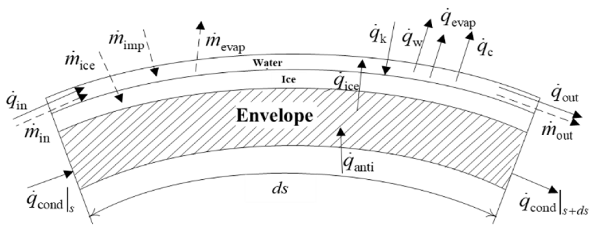
2. Computational Methodology

2.1. Approximate Solution for Wing Surface Heat Transfer Coefficient

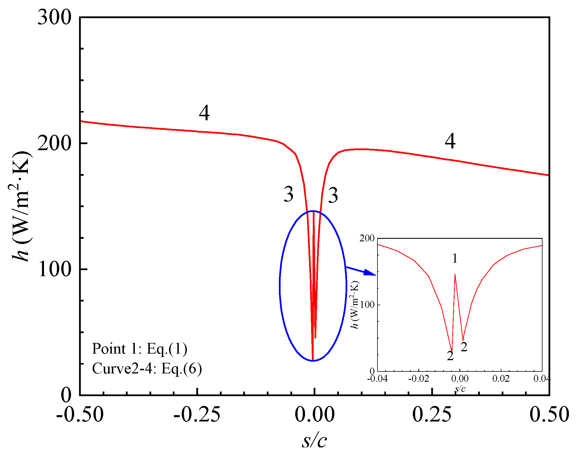
The convective heat transfer coefficient (h) on wing surfaces correlates with airflow dynamics and physical properties. h is solved through the following approximations according to the boundary layer integral method:

 (1) 

Stagnation Region Treatment

Near the leading-edge stagnation zone, it is approximated as airflow around a cylinder with equivalent diameter D (twice the leading-edge curvature radius). h is calculated using cylinder-specific formulas:

For laminar flow [21],

$$h=1.14{\displaystyle \frac{{\lambda }_0}{D}}{\left(R{e}_D\right)}^{0.5}{P}_r^{0.4}$$

(1)

where D refers to the cylinder diameter, λ₀ refers to air thermal conductivity, Pr is the Prandtl number (0.72 at 0 °C), μ₀ is the air dynamic viscosity, ρ₀ is the air density, and V₀ denotes freestream velocity. $R{e}_D$ is the Reynolds number (D-based), yielding

$$R{e}_D={\displaystyle \frac{{\rho }_0{V}_{0}D}{\mu }}$$

(2)

For turbulent flow [22],

$$h=0.063{\displaystyle \frac{{\lambda }_0}{D}}{\left(R{e}_D\right)}^{0.8}{P}_r^{1/3}$$

(3)

 (2) 

Non-Stagnation Region Treatment

Regions beyond the leading edge are modeled as flat plates:

For laminar flow [23],

$$h=0.332{\left(R{e}_s\right)}^{0.5}\cdot P_r^{1/3}\cdot {\displaystyle \frac{\lambda }{s}}$$

(4)

$$R{e}_s={\displaystyle \frac{{\rho }_0{V}_{0}S}{\mu }}$$

(5)

S denotes the surface distance from the stagnation point of the leading edge of the airfoil.

For turbulent flow [24],

$$h=0.0296{\displaystyle \frac{\lambda }{S}}{\left(R{e}_s\right)}^{0.8}{P}_r^{1/3}$$

(6)

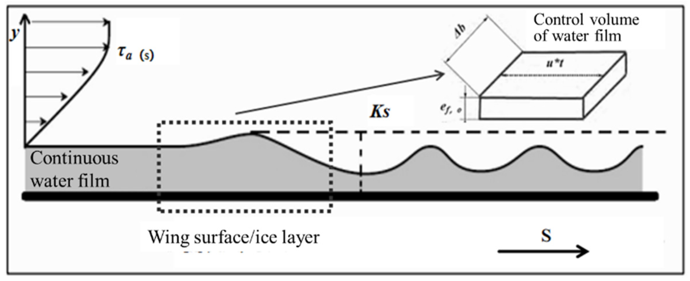
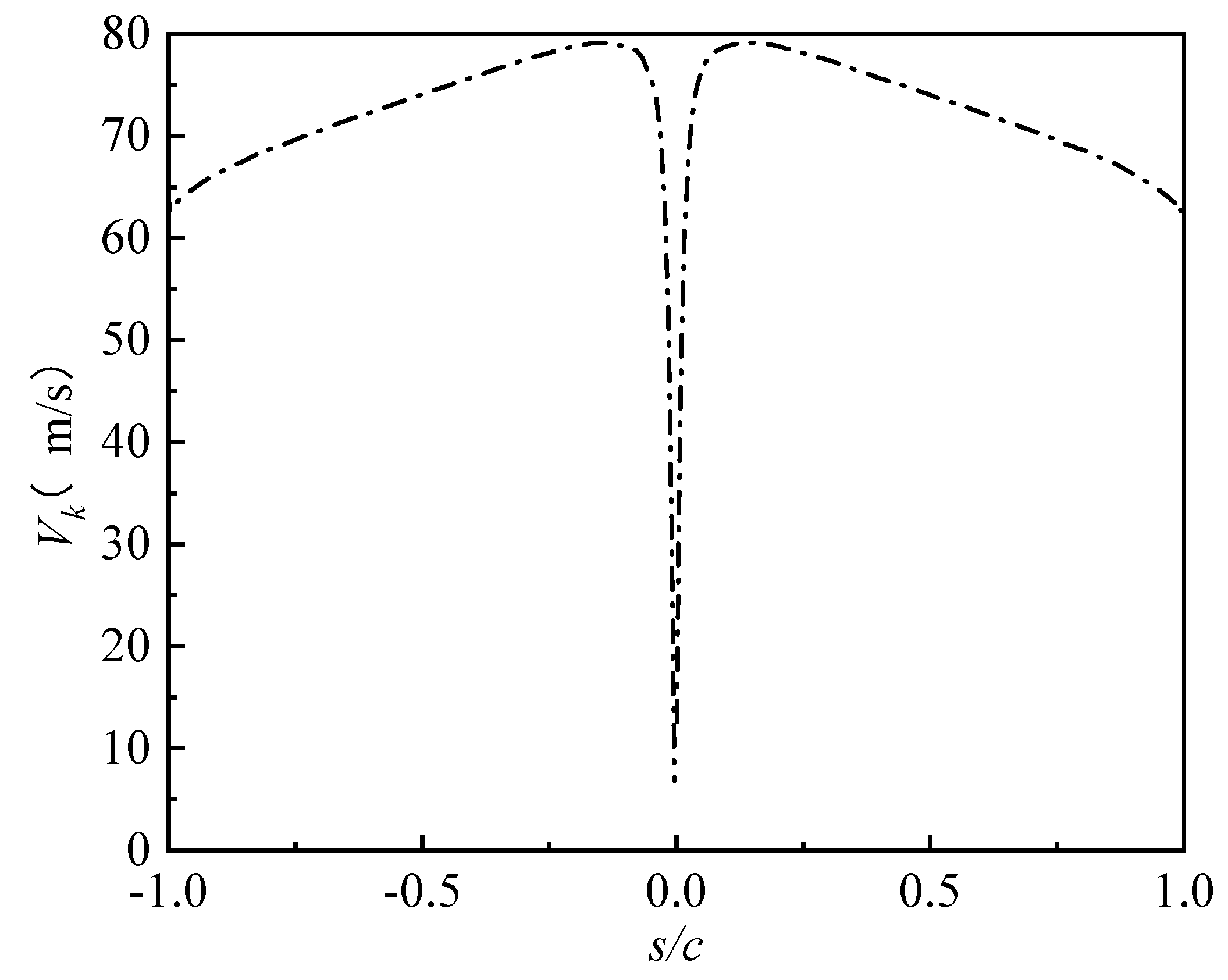
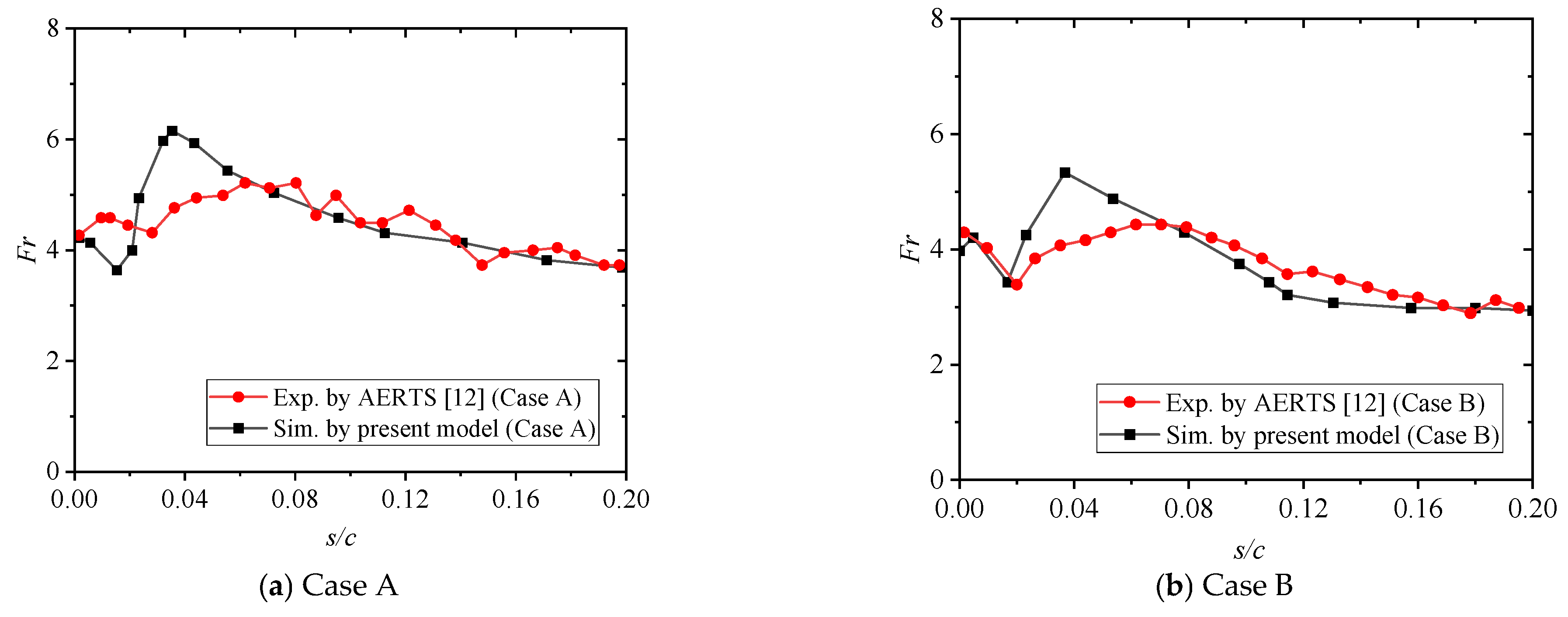
2.2. Roughness Reynolds Number

The flow dynamics over ice-accreted airfoil surfaces exhibit significant complexity, characterized by an intricate laminar-to-turbulent transition process. Precise determination of the transition point location is essential for flow regime classification. To address this, the roughness Reynolds number (Re_k) is introduced [25]:

$$R{e}_k={\displaystyle \frac{V_k{K}_s}{{\mu }_0}}$$

(7)

where

• K_s denotes the surface roughness height (varying spatially along the airfoil);
• V_k represents the airflow velocity at the roughness element height.

Through Equation (7), the Re_k distribution across the airfoil surface under specified conditions can be established. The transition location is subsequently determined by comparing Re_k against the critical Reynolds number Re_c. As illustrated in Figure 2, distinct flow patterns emerge across the transition point. Post-transition flow exhibits pronounced velocity gradients that generate vortical structures, enhancing local turbulent mixing and consequently elevating thermal exchange efficiency in the affected region. The critical Reynolds number (Re_c) is empirically assigned a value of 600 for the laminar-to-turbulent transition [26].

The equivalent sand grain roughness height (K_s) exhibits significant variation across ice-contaminated airfoil surfaces. Determination of K_s magnitudes characterizing water films, beads, and rivulets is achieved through coupled heat/mass transfer analysis and hydrodynamic force balance on wall-bounded control volume elements. Under relatively high-temperature icing conditions (glaze ice regime), supercooled droplets impinging on the airfoil do not undergo instantaneous freezing. As illustrated in Figure 3, aerodynamic shear forces induce undulation and coalescence of surface water into continuous liquid films, where the film thickness constitutes the primary source of surface roughness, thereby defining the K_s value.

The aerodynamic shear stress (τ_i) acting on a water film control volume is defined as follows:

$${\tau }_{\mathrm{i}}={ \mathsf{\mu }}_{\mathrm{w}}{\displaystyle \frac{\mathrm{d}u}{\mathrm{dy}}}$$

(8)

where

• ${\mu }_{\mathrm{w}}$ = dynamic viscosity of water;
• u = horizontal component of velocity;
• y = film thickness.

According to Shin et al.’s equivalent roughness model [15,28], K_s is empirically computed as follows:

$$\begin{array}{c}{K}_{\mathrm{s},\mathrm{s}h\mathrm{in}}=\left[0.5714+0.2457LWC+1.2571LW{C}^2\right]\cdot \\ \hspace{1em}\hspace{1em}\hspace{1em}\left(0.047T_{\infty }-11.27\right)\cdot \left(0.4286+0.0044139{\mathrm{u}}_{\infty }\right)\\ 0.001177\cdot c\end{array}$$

(9)

where c denotes the chord length of the airfoil. It should be noted that the expression does not account for the effect of time on the ice roughness. Applying the boundary conditions y = 0 and u = 0 to Equation (9) yields the velocity profile:

$$u={\displaystyle \frac{{\tau }_{\mathrm{i}}}{{\mathsf{\mu }}_{\mathrm{w}}}}\mathrm{y}$$

(10)

The average velocity $\overline{u}$ and accumulated water mass $m_{\mathrm{w}}$ are then derived:

$$\overline{u}={\displaystyle \frac{1}{2}}{e}_{\mathrm{f},\mathrm{o}}{\displaystyle \frac{{\tau }_i}{{\mu }_w}}$$

(11)

$$m_{\mathrm{w}}={\rho }_{\mathrm{w}}\Delta b{e}_{\mathrm{f},\mathrm{o}}u$$

(12)

where ${\rho }_{\mathrm{w}}$ denotes water density, Δb is the control volume width, and $e_{\mathrm{f},\mathrm{o}}$ = film thickness. For simple airfoils, Δb ≈ 1.

The water mass accumulation m_w combines CFD-derived collection efficiency β (insensitive to K_s and mesh resolution) with impingement limits:

$$m_{\mathrm{w}}=\underset{s_{\mathrm{i}}}{\overset{s_{\mathrm{u}}}{{\displaystyle \int }}}\left(u·\beta ·LWC\right)d\mathrm{s}$$

(13)

Film thickness and roughness height are given by

$$e_{\mathrm{f},\mathrm{o}}=\sqrt{{\displaystyle \frac{2{\mu }_{\mathrm{w}}{\mathrm{m}}_{\mathrm{w}}}{{\tau }_{\mathrm{i}}{\mathsf{\rho }}_{\mathrm{w}}}}}$$

(14)

$$K_s={\displaystyle \frac{3}{4}}{\displaystyle \frac{{\tau }_i}{{\mu }_w}}\sqrt{{\displaystyle \frac{e_{f,o}^3}{g}}}$$

(15)

Parametric analysis of the governing expressions reveals that surface roughness magnitude within water film regimes is primarily dictated by two coupled mechanisms: (i) aerodynamic shear stress (τ_i) acting at the air–liquid interface, which serves as the dominant driver of interfacial instability and roughness evolution, and (ii) intrinsic fluid properties—notably dynamic viscosity (μ_w) governing momentum diffusion, density (ρ_w) modulating inertial resistance, and phase interaction characteristics. A rigorous derivation of the shear stress quantification methodology, establishing closed-form correlations between aerodynamic forcing functions and interfacial morphology, will be presented in the following section.

 (1) 

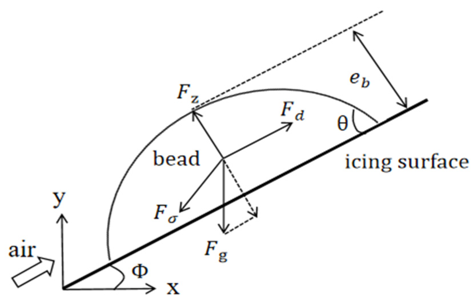
Roughness of Water Droplets and Fine Flow Areas

Under aerodynamic shear forces, continuous water films undergo fragmentation, transitioning into discrete beads or rivulets. As schematically illustrated in Figure 4, beads on ice surfaces maintain quasi-static equilibrium through the balance of three critical forces.

Neglecting aerodynamic lift forces, we assume beads maintain adhesion to the ice surface without detachment. The aerodynamic drag force acting on a bead is quantified as

$$F_{\mathrm{d}}={ \mathsf{\rho }}_0{\mathrm{C}}_{\mathrm{d}}{\mathrm{A}}_{\mathrm{b}}\left|{\mathrm{V}}_0\right|{\mathrm{V}}_0/2$$

(16)

The parameters are as follows:

• C_d = 0.44—the drag coefficient (constant for spherical beads);
• A_b is the frontal area exposed to airflow.

$${\mathrm{A}}_{\mathrm{b}}=\left({\mathsf{\theta }}_{\mathrm{c}}-{\displaystyle \frac{1}{2}}\sin 2{\mathsf{\theta }}_{\mathrm{c}}\right){\displaystyle \frac{{\mathrm{e}}_{\mathrm{b}}^2}{{\left(1-{ \cos \mathsf{\theta }}_{\mathrm{c}}\right)}^2}}$$

(17)

The variables are as follows:

• e_b is the bead height (equilibrium vertical dimension);
• θ_c is the surface contact angle.

The capillary force is derived through azimuthal integration:

$$F_{\mathsf{\sigma }}={\int }_0^{2\pi }{\mathsf{\sigma }}_{\mathrm{d}}\cos \mathsf{\theta }\cos \mathsf{\phi }\mathrm{r} \mathrm{d}\mathsf{\phi }$$

(18)

where r is the basal radius of the bead–substrate interface.

$$r= \sin {\theta }_{\mathrm{c}}{\mathrm{e}}_{\mathrm{b}}/\left(1- \cos {\theta }_{\mathrm{c}}\right)$$

(19)

where θ and $\phi$ are the local contact angle and inclination angle, respectively.

The linear constraints of both parameters with the boundary layer temperature are illustrated in Figure 5. The contact angle θ between water beads and ice surfaces is dually constrained by the boundary layer temperature and surface inclination angle. As the temperature increases, θ gradually decreases to a minimum near 5 °C and then increases sharply until the integrated droplet morphology can no longer be maintained. This variation follows a simple cosine distribution, where Δθ_c in the figure denotes the hysteresis angle of the water bead–wall contact.

The gravitational component along the tangential direction of the ice surface is expressed as follows:

$$F_{\mathrm{g}}={ \mathsf{\rho }}_{\mathrm{w}}{V}_w\mathrm{g}\left|\sin \mathsf{\phi }\right|$$

(20)

where V_w denotes the volume of the water bead. The bead volume is calculated by the following:

$$V_w={\displaystyle \frac{\pi }{3}}{\displaystyle \frac{2+ \cos {\theta }_{\mathrm{c}}}{1- \cos {\theta }_{\mathrm{c}}}}{e}_{\mathrm{b}}^3$$

(21)

Combining the above equations yields the force balance equation:

$$F_{\mathrm{d}}+F_{\mathsf{\sigma }}+F_{\mathrm{g}}=0$$

(22)

After obtaining the velocity and temperature distributions in the boundary layer over the ice surface, the roughness value of the bead zone is determined as follows:

$$K_s=e_{\mathrm{b}}$$

(23)

 (2) 

Roughness Demarcation Method Based on Critical Friction Coefficient

Experimental studies reveal that distinct water phase distributions characterize different regions of ice surfaces. Liquid water films predominantly exist in the frontal zone of the ice interface, micro-droplets accumulate in the transition region between the water film and critical impingement point, and overflow water forms in areas beyond the impingement range. Within ice surface roughness prediction models, precise demarcation of phase transition boundaries critically influences the calculation of surface morphological characteristics. By applying the principle of fluid interface mechanical equilibrium, quantitative division of distinct phase regions through analysis of the liquid film’s force state is achieved.

(a)

Boundary Between Water Film and Droplets

During ice surface expansion, the liquid water film experiences dual effects: aerodynamic shear forces and interfacial cohesive forces dominated by surface tension. According to kinetic equilibrium conditions, the liquid film maintains a continuous flow state when aerodynamic shear forces overcome interfacial cohesive forces. Conversely, when mechanical equilibrium reverses, surface tension governs droplet coalescence. Therefore, the critical phase transition condition for water film–droplet transformation (mobile phase) can be determined by establishing a mechanical equilibrium model of the liquid film. Through hydrodynamic theory, the development of a shear stress calculation model quantitatively characterizes this phase transition mechanism.

$${\tau }_{\mathrm{i}}=C_{\mathrm{f}}{\displaystyle \frac{1}{2}}{\rho }_0{u}^2{A}_{\mathrm{i}}$$

(24)

where A_i denotes the surface area of the water film (m²), and C_f represents the friction coefficient, obtainable through empirical formulations. The friction coefficient [30] is determined as follows:

$${\mathrm{C}}_{\mathrm{f}}={\left[3.476+0.707\ln \left({\mathrm{K}}_{\mathrm{s},\mathrm{s}h\mathrm{in}}/\mathrm{s}\right)\right]}^{-2.46}$$

(25)

where $K_{\mathrm{s},\mathrm{s}h\mathrm{in}}/\mathrm{s}$ is the dimensionless roughness parameter. The cohesive force induced by surface tension is quantified as

$${\tau }_{\mathsf{\sigma }}=\sigma \left(1- \cos {\theta }_{\mathrm{c}}\right)S_{\mathsf{\sigma }}$$

(26)

where τ_σ is the cohesive force within the water film, and S_σ denotes the perimeter of the water film. For two-dimensional problems, assuming a control element width of unity, the condition ${\tau }_{\mathrm{i}} \ge {\tau }_{\mathsf{\sigma }}$ yields

$${\mathrm{C}}_{\mathrm{f}} ⩾ {\displaystyle \frac{2\mathsf{\sigma }}{{\mathsf{\rho }}_0{\mathrm{u}}^2}} \left(1-{\cos \mathsf{\theta }}_{\mathrm{c}}\right)$$

(27)

We define the critical friction coefficient $C_{\mathrm{f},\mathrm{c}}$ as

$${\mathrm{C}}_{\mathrm{f},\mathrm{c}}={\displaystyle \frac{2\mathsf{\sigma }}{{\mathsf{\rho }}_0{\mathrm{u}}^2}} \left(1-{ \cos \mathsf{\theta }}_{\mathrm{c}}\right)$$

(28)

When ${\mathrm{C}}_{\mathrm{f}} ⩾{ \mathrm{C}}_{\mathrm{f},\mathrm{c}}$, the surface roughness sustains a continuous water film. Conversely, the film coalesces into discrete droplets.

(b)

Boundary Between Droplets and Overflow Streams

If the water film transitions into droplets before reaching the impingement limit while overflow occurs beyond this limit, the liquid water manifests as micro-streams. Consequently, the phase boundary between droplets and micro-streams corresponds precisely to the droplet impingement limit.

3. Results and Discussion

Dynamic analysis of water droplet behavior on the airfoil surface revealed the roughness distribution characteristics across distinct zones of the ice-accreted surface. For model validation, the K_s values derived through the boundary layer integration methodology were rigorously benchmarked against experimental data from the Adverse Environment Rotor Test Stand (AERTS) facility [17]. The investigation employed an NACA0012 airfoil configuration with a characteristic chord length of 0.5334 m. Computational test conditions are systematically detailed in

Table 1. Verification cases of surface roughness and heat transfer coefficient.

Parameter	Case A	Case B
Airfoil	NACA0012	NACA0012
Characteristic length, m	0.5334	0.5334
Angle of attack (AoA), °	0	0
Velocity, m/s	66.7	66.7
Temperature, °C	−3.6	−5.86
LWC, g/m3	1.7	1.0
Droplet median volume diameter (MVD), μm	30	20
Time, s	100	100

.

Essential parameters including the surface distance S and local velocity V_k of the airfoil must be determined to compute the local heat transfer coefficient. These parameters exhibit dual dependencies on both the specific airfoil geometry and the prevailing flight conditions. Using the canonical NACA0012 airfoil as an exemplar, the solution methodology is elucidated. The corresponding airfoil coordinates, delineating upper and lower surface profiles, are tabulated in

Table 2. Airfoil coordinate points.

xupper	yupper	xlower	ylower
0.000	0.000	0.000	0.000
0.054	0.037	0.086	−0.044
0.114	0.049	0.146	−0.053
0.174	0.055	0.206	−0.057
0.234	0.058	0.266	−0.059
0.294	0.059	0.326	−0.059
0.354	0.059	0.386	−0.058
0.414	0.057	0.446	−0.055
0.474	0.054	0.506	−0.052
0.534	0.050	0.566	−0.048
0.594	0.045	0.626	−0.043
0.654	0.040	0.686	−0.037
0.714	0.034	0.746	−0.031
0.774	0.028	0.806	−0.025
0.834	0.021	0.866	−0.018
0.894	0.014	0.926	−0.010
0.954	0.006	0.986	−0.002
1.000	0.000	1.000	0.000

.

The surface distance S is measured from the stagnation point at the leading edge and computed as follows:

$$\Delta {\mathrm{S}}_{\mathrm{i}}=\sqrt{{\left({\mathrm{x}}_{\mathrm{i} +1}-{ \mathrm{x}}_{\mathrm{i}}\right)}^2+{\left({\mathrm{y}}_{\mathrm{i} +1}-{ \mathrm{y}}_{\mathrm{i}}\right)}^2}$$

(29)

$${\mathrm{S}}_{\mathrm{i}}=\sum \Delta {\mathrm{S}}_{\mathrm{i}}$$

(30)

This method approximates curved segments with straight lines. A more precise approach utilizes circular arcs to represent actual curves, yielding higher accuracy at the cost of increased computational complexity. For widely used low-drag airfoils, the curvature radius is sufficiently large (i.e., curvature is small) except near the leading-edge stagnation point. Consequently, straight-line approximation introduces negligible errors (<2% relative error for NACA0012, where the leading-edge radius is ~1% chord length), satisfying engineering precision requirements for routine calculations.

Surface velocity distribution on the airfoil may be obtained via airfoil theory or wind tunnel testing, typically presented as pressure coefficient (C_p) distributions. Figure 6 illustrates the C_p distribution for NACA0012 at AoA = 0°.

The pressure coefficient is defined as

$$C_{\mathrm{p}}={\displaystyle \frac{p_1-p_0}{0.5{\mathsf{\rho }}_0{V}_0^2}}$$

(31)

where p₀ denotes the freestream static pressure, V₀ is the freestream velocity, and p₁ is the local static pressure at the boundary layer outer edge.

Since C_p characterizes the local pressure distribution, the local velocity V_k can be derived from it. For an anti-icing system design for civil aircraft, air compressibility effects are negligible, especially for the flow near the boundary layer. Thus, Bernoulli’s equation for incompressible flow yields

$$p_0+{\displaystyle \frac{{\mathsf{\rho }}_0{\mathrm{V}}_0^2}{2}}=p_1+{\displaystyle \frac{{\mathsf{\rho }}_0{\mathrm{V}}_k^2}{2}}$$

(32)

$${\displaystyle \frac{{\mathrm{V}}_{\mathrm{i}}}{{\mathrm{V}}_0}}=\sqrt{1-{ \mathrm{C}}_{\mathrm{p}}}$$

(33)

The local temperature yields

$$T_k=T_0+{\displaystyle \frac{V_0^2-V_k^2}{2C_0}}$$

(34)

where

• T₀ = freestream temperature (°C);
• V₀ = freestream velocity (m/s);
• C₀ = isobaric specific heat capacity of air (J/kg·°C).

Figure 7 shows a flowchart of the proposed methods. According to the flowchart, the resulting local velocity distribution near the boundary layer for NACA0012 under this operating condition is as presented in Figure 8.

The distribution of equivalent sand grain roughness height (K_s) over the NACA0012 airfoil surface under this operating condition was obtained using the local roughness determination method proposed above and subsequently compared with experimental data and the Shin roughness model. As shown in Figure 9, the computational results from the local roughness model exhibit a chordwise K_s distribution characterized by an initial increase followed by a gradual decrease, with the peak value occurring at s/c = 2%. A slight discrepancy is observed between the calculated and experimental peak Ks values, attributable to the model’s assumption that hemispherical water droplets uniformly cover the entire roughness zone while neglecting actual droplet density distribution and flow dynamics. Under real icing conditions, the water film is rapidly redistributed during initial ice accretion, preventing complete droplet coverage of the airfoil’s rough surface, thereby resulting in lower experimental roughness heights compared to computational predictions. Figure 9 further reveals that the wetted region computed by the local roughness model extends beyond experimental measurements. This deviation stems from centrifugal forces—induced by the rotational velocity control system used in experiments—causing spanwise water film migration, an effect not accounted for in the zonal roughness treatment method. In contrast, the Shin roughness model generates only a single specific K_s distribution per operating condition, demonstrating significant deviations from experimental values that substantially compromise the accuracy of subsequent heat transfer coefficient calculations.

The distribution of $R{e}_k$ over the wing surface was calculated and comparatively analyzed with $R{e}_c$, yielding the flow regime distribution and transition location on the wing surface. The relative magnitude relationship between these parameters is illustrated in Figure 10. Only in minimal regions near the leading and trailing edges (transition occurring at approximately 0.1% chord length from the leading edge) does the airflow maintain laminar state, while the majority of the wing surface exhibits turbulent flow. This phenomenon is intrinsically linked to the elevated surface roughness under actual icing conditions.

Following the determination of Re_k distribution, the heat transfer coefficient profiles were computed separately for the stagnation region and the laminar/turbulent zones along the leading edge. As shown in Figure 11, the most significant flow stagnation occurs at the wing leading edge—where the velocity gradient reaches its maximum—resulting in a peak heat transfer coefficient under AoA equal to 0°. Progressing from the stagnation point toward the trailing edge, the flow transitions from a brief laminar state to a turbulent regime within an extremely short distance. As a result, for practical anti-icing operations, the heat transfer coefficients across the wing surface (excluding the stagnation region) can be uniformly calculated using turbulent flat plate correlations. From an engineering perspective, due to the complexity of pointwise local heat transfer coefficient calculations, the average heat transfer coefficient h_ave is typically employed for anti-icing system design, expressed as follows:

$$h_{\mathrm{ave}}={\displaystyle \frac{1}{\mathrm{S}}}{{\displaystyle \int }}_0^{\mathrm{s}}h\mathrm{ds}$$

(35)

It should be noted that a precise knowledge of the heat transfers associated with a specific roughness pattern is key to ensuring reliable numerical icing predictions. Ignatowicz et al. [31] concluded that roughness height K_s is the most sensitive parameter, responsible for about 90% of the changes in ice thickness and extension. The K_s correlation in Equation (9) is empirical based on experimental data reported by Ruff and Berkowitz [14]. As a result, it is necessary to reinforce the experimental databases by precisely measuring the heat transfer variations induced by typical ice roughness.

The dimensionless number Fr yields

$$Fr={\displaystyle \frac{Nu}{\sqrt{R{e}_k}}}$$

(36)

Figure 12 depicts the Fr behavior on the surface of the NACA0012 airfoil. The Fr curve obtained using the proposed method exhibits similar trends to experimental results regarding transition onset. Both calculated and experimental transition locations occur near s/c = 2%. The computational model predicts higher heat transfer rates, which is attributed to the partitioned boundary layer integral method predicting increased roughness in laminar flow regions. Elevated K_s values consequently lead to enhanced heat transfer, resulting in larger Fr values at the airfoil’s trailing edge in computational predictions.

4. Conclusions

The present study extends the traditional boundary layer integral method by developing a partitioned-theory-based rough-wall boundary layer integral approach, which accounts for roughness variations induced by droplet morphologies. Computational validation using the NACA0012 airfoil demonstrates favorable agreement with experimental data. The major conclusions are as follows:

(1)

A method for the rapid prediction of the heat transfer coefficient on icing surfaces of aircraft wings based on a partitioned rough-wall boundary layer integral approach was proposed. It enables calculation of the heat transfer coefficient through airfoil geometry without the need for CFD computations.

(2)

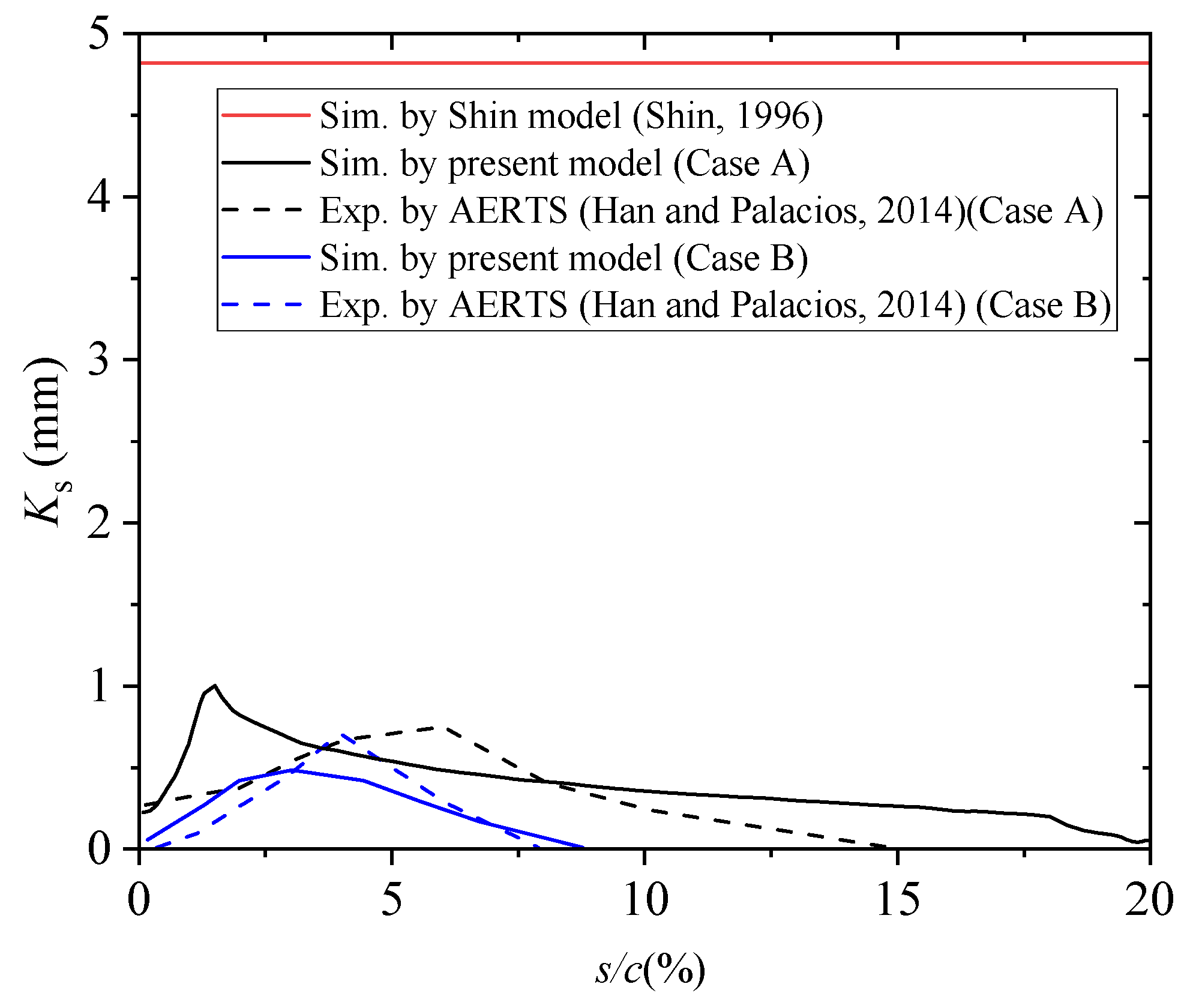
Three distinct hydrodynamic regimes—a hydraulically smooth zone (water film), a transitionally rough zone (water beads), and a fully rough zone (rivulets)—are categorized by the partitioned theory method based on droplet dynamics. Each regime exhibits specific equivalent sand grain roughness heights. This framework enables determination of the relative magnitude between roughness Reynolds number and critical Reynolds number, thereby mapping the Ks distribution over the aerodynamic surface.

(3)

Incorporating local roughness effects, the refined boundary layer integral method computes convective heat transfer coefficients along the wing surface. Compared to conventional approaches, the boundary layer transition is identified at the 0.1 chordwise station (0.1 s/c).

(4)

The convective heat transfer distribution over the NACA0012 airfoil is quantitatively characterized by the proposed method. It shows that prediction accuracy for heat transfer coefficients shows measurable improvement.

References

1. Bragg, M.B.; Broeren, A.P.; Blumenthal, L.A. Iced-airfoil aerodynamics. Prog. Aerosp. Sci. 2005, 41, 323–362. [Google Scholar] [CrossRef]
2. Liu, Y.; Wang, Q.; Yi, X.; Chen, N.; Ren, J.; Li, W. An anti-icing scaling method for wind tunnel tests of aircraft thermal ice protection system. Chin. J. Aeronaut. 2024, 37, 1–6. [Google Scholar] [CrossRef]
3. Liu, Y.; Yang, Q.; Wang, Q.; Guo, X.; Bu, X.; Yi, X. Investigations on Optimization and Verification of Nacelle Hot Air Anti-Icing System in a Large Icing Wind Tunnel. Aerosp. Sci. Technol. 2025, 163, 110312. [Google Scholar] [CrossRef]
4. Aliaga, C.N.; Aubé, M.S.; Baruzzi, G.S.; Habashi, W.G. FENSAP-ICE-Unsteady: Unified in-flight icing simulation methodology for aircraft, rotorcraft, and jet engines. J. Aircr. 2011, 48, 119–126. [Google Scholar] [CrossRef]
5. Verdin, P.G.; Charpin, J.P. Multi-stepping ice prediction on cylinders and other relevant geometries. J. Aircr. 2013, 50, 871–878. [Google Scholar] [CrossRef]
6. Cao, Y.; Ma, C.; Zhang, Q.; Sheridan, J. Numerical simulation of ice accretions on an aircraft wing. Aerosp. Sci. Technol. 2012, 23, 296–304. [Google Scholar] [CrossRef]
7. Lavoie, P.; Pena, D.; Hoarau, Y.; Laurendeau, E. Comparison of thermodynamic models for ice accretion on airfoils. Int. J. Numer. Methods Heat Fluid Flow. 2018, 28, 1004–1030. [Google Scholar] [CrossRef]
8. Zhang, Y.; Yuan, X.; Xiong, J.; Bu, X. An Electro-thermal De-icing Model and Simulation Analysis Considering Ice Shedding. Trans. Nanjing Univ. Aeronaut. Astronaut. 2025, 42, 162–177. [Google Scholar]
9. Ferro, C.G.; Pietrangelo, F.; Maggiore, P. Heat exchange performance evaluation inside a lattice panel using CFD analysis for an innovative aerospace anti-icing system. Aerosp. Sci. Technol. 2023, 141, 108565. [Google Scholar] [CrossRef]
10. Yakhya, S.; Ernez, S.; Morency, F. Computational fluid dynamics investigation of transient effects of aircraft ground deicing jets. J. Thermophys. Heat Transf. 2019, 33, 117–127. [Google Scholar] [CrossRef]
11. Ozcer, I.A.; Baruzzi, G.S.; Reid, T.; Habashi, W. FENSAP-ICE: Numerical prediction of ice roughness evolution, and its effects on ice shapes. SAE Tech. Pap. 2011. [Google Scholar] [CrossRef]
12. Bayeux, C.; Radenac, E.; Villedieu, P. Theory and validation of a 2D finite-volume integral boundary-layer method for icing applications. AIAA J. 2019, 57, 1092–1112. [Google Scholar] [CrossRef]
13. Harry, R.; Radenac, E.; Blanchard, G.; Villedieu, P. Heat Transfer modeling by integral boundary-layer methods towards icing applications. In Proceedings of the AIAA AVIATION 2021 FORUM, VIRTUAL EVENT, 2–6 August 2021. [Google Scholar]
14. Ruff, G.A.; Berkowitz, B.M. Users Manual for the NASA Lewis Ice Accretion Prediction Code (LEWICE); Sverdrup Technology, Inc.: Brook Park, OH, USA, 1990. [Google Scholar]
15. Shin, J. Characteristics of surface roughness associated with leading-edge ice accretion. J. Aircr. 1996, 33, 316–321. [Google Scholar] [CrossRef]
16. Hansman Jr, R.J.; Turnock, S.R. Investigation of surface water behavior during glaze ice accretion. J. Aircr. 1989, 26, 140–147. [Google Scholar] [CrossRef]
17. Han, Y.; Palacios, J. Transient heat transfer measurements of surface roughness due to ice accretion. In Proceedings of the 6th AIAA Atmospheric and Space Environments Conference, Atlanta, GA, USA, 16–20 June 2014. [Google Scholar]
18. Steiner, J.; Bansmer, S. Ice roughness and its impact on the ice accretion process. In Proceedings of the 8th AIAA Atmospheric and Space Environments Conference, Washington, DC, USA, 13–17 June 2016. [Google Scholar]
19. Mcclain, S.T.; Vargas, M.; Tsao, J.; Broeren, A.; Lee, S. Ice accretion roughness measurements and modeling. In Proceedings of the European Conference for Aeronautics and Space Sciences (EUCASS), Milan, Italy, 3–6 July 2017. [Google Scholar]
20. Yamaguchi, K.; Hansman, R.J., Jr. Heat transfer on accreting ice surfaces. J. Aircr. 1992, 29, 108–113. [Google Scholar] [CrossRef]
21. Martinelli, R.C. An Investigation of Aircraft Heaters: VIII-A Simplified Method for the Calculation of the Unit Thermal Conductance Over Wings. National Advisory Committee for Aeronautics. 1943. Available online: https://ntrs.nasa.gov/citations/19930092970 (accessed on 14 July 2025).
22. Goldstein, K.; Novoselac, A. Convective heat transfer in rooms with ceiling slot diffusers (RP-1416). HVACR Res. 2010, 16, 629–655. [Google Scholar] [CrossRef]
23. Blasius, H. Grenzschichten in Flüssigkeiten Mit Kleiner Reibung; Druck von BG Teubner: Leipzig, Germany, 1907. [Google Scholar]
24. Kolev, N.I. Multiphase Flow Dynamics; Springer: Berlin/Heidelberg, Germany, 2007. [Google Scholar]
25. Department of Transportation; FAA. 14 CFR Appendix O to Part 25—Supercooled Large Drop Icing Conditions; FAA: Washington, DC, USA, 2014. [Google Scholar]
26. Özgen, S.; Canıbek, M. Ice accretion simulation on multi-element airfoils using extended Messinger model. Heat Mass Transf. 2009, 45, 305–322. [Google Scholar] [CrossRef]
27. Rodič, P. Modelna Podobnost in Vpliv Modelnega Merila na Prenos Rezultatov Fizičnega Hidravličnega Modela na Prototip: Magistrsko Delo [na Spletu]. Master’s Thesis, Ljubljana, Slovenia, 2016. Available online: https://repozitorij.uni-lj.si/IzpisGradiva.php?lang=slv&id=88894 (accessed on 15 July 2025).
28. Shin, J.; Berkowitz, B.; Chen, H.; Cebeci, T. Prediction of ice shapes and their effect on airfoil performance. In Proceedings of the Aerospace Sciences Meeting, Reno, NV, USA, 7–10 January 1991. [Google Scholar]
29. Guo, W.; Shen, H.; Li, Y.; Feng, F.; Tagawa, K. Wind tunnel tests of the rime icing characteristics of a straight-bladed vertical axis wind turbine. Renew. Energy 2021, 179, 116–132. [Google Scholar] [CrossRef]
30. Wen, T.; Agarwal, R.K. A new extension of wray-agarwal wall distance free turbulence model to rough wall flows. In Proceedings of the AIAA Scitech 2019 Forum, San Diego, CA, USA, 7–11 January 2019. [Google Scholar]
31. Ignatowicz, K.; Morency, F.; Beaugendre, H. Sensitivity study of ice accretion simulation to roughness thermal correction model. Aerospace 2021, 8, 84. [Google Scholar] [CrossRef]
Figure 1. Mass and energy conservation for a differential element on anti-icing surfaces [8].
Aerospace 12 00634 g001
Figure 2. Flow distribution of boundary layer near the flat plates [27].
Aerospace 12 00634 g002
Figure 3. Schematic of the roughness height in the water film flow zone.
Aerospace 12 00634 g003
Figure 4. Diagram of force acting on water droplets [29].
Aerospace 12 00634 g004
Figure 5. Relation between temperature of the boundary layer, contact angle, and inclination angle.
Aerospace 12 00634 g005
Figure 6. Pressure coefficient curve (Case A).
Aerospace 12 00634 g006
Figure 7. Flowchart of the proposed method for h prediction.
Aerospace 12 00634 g007
Figure 8. Local velocity near the boundary layer (Case A).
Aerospace 12 00634 g008
Figure 9. Comparison of different roughness models with experimental values [12,15].
Aerospace 12 00634 g009
Figure 10. Roughness Reynolds number (Case A).
Aerospace 12 00634 g010
Figure 11. h behavior on the surface of NACA0012 airfoil (Case A).
Aerospace 12 00634 g011
Figure 12. Fr behavior on the surface of NACA0012 airfoil.
Aerospace 12 00634 g012