Article

Visual Detection on Aircraft Wing Icing Process Using a Lightweight Deep Learning Model

School of Aeronautics and Astronautics, Sun Yat-Sen University, Shenzhen 518000, China
*
Author to whom correspondence should be addressed.
These authors contributed equally to this work.
Aerospace 2025, 12(7), 627; https://doi.org/10.3390/aerospace12070627
Submission received: 30 May 2025 / Revised: 3 July 2025 / Accepted: 10 July 2025 / Published: 12 July 2025
(This article belongs to the Section Aeronautics)

Abstract

Aircraft wing icing significantly threatens aviation safety, causing substantial losses to the aviation industry each year. High transparency and blurred edges of icing areas in wing images pose challenges to wing icing detection by machine vision. To address these challenges, this study proposes a detection model, Wing Icing Detection DeeplabV3+ (WID-DeeplabV3+), for efficient and precise aircraft wing leading edge icing detection under natural lighting conditions. WID-DeeplabV3+ adopts the lightweight MobileNetV3 as its backbone network to enhance the extraction of edge features in icing areas. Ghost Convolution and Atrous Spatial Pyramid Pooling modules are incorporated to reduce model parameters and computational complexity. The model is optimized using the transfer learning method, where pre-trained weights are utilized to accelerate convergence and enhance performance. Experimental results show WID-DeepLabV3+ segments the icing edge at 1920 × 1080 within 0.03 s. The model achieves the accuracy of 97.15%, an IOU of 94.16%, a precision of 97%, and a recall of 96.96%, representing respective improvements of 1.83%, 3.55%, 1.79%, and 2.04% over DeeplabV3+. The number of parameters and computational complexity are reduced by 92% and 76%, respectively. With high accuracy, superior IOU, and fast inference speed, WID-DeeplabV3+ provides an effective solution for wing-icing detection.

1. Introduction

Flight safety is a fundamental concern in the aviation field. Under specific meteorological conditions, icing is a significant factor threatening flight safety. When an aircraft encounters supercooled large droplets or flies through clouds containing ice crystals, ice may accumulate on the leading edge of the aircraft wing surface. This accumulation alters the aerodynamic performance of the aircraft, reducing maneuverability and stability and posing a severe threat to flight safety [1].
Aircraft accidents caused by icing are not uncommon. According to statistical data from the U.S. National Transportation Safety Board, 583 aircraft icing-related incidents occurred between 1982 and 2000, resulting in 819 fatalities [2]. Between 2003 and 2006, 380 additional wing-icing-related flight accidents were recorded in the United States. Since 2007, China has also experienced several icing-related flight accidents.
The icing detector plays a crucial role in an aircraft’s anti-icing and de-icing system, significantly enhancing modern large passenger aircraft’s safety, efficiency, and technological advancement. Currently, single-point icing detectors are commonly used for monitoring icing conditions. Traditional single-point icing detection methods include the flat-film vibration method, differential pressure method, radioactive isotope detection, infrared radiation reflection, and fiber-optic reflection detection.
The vibration method determines icing conditions by monitoring changes in sensor vibration frequency after ice formation [3]. The flat-film resonance method detects icing by analyzing changes in mass and stiffness when ice accumulates on the film surface. The differential pressure method identifies icing by measuring the engine inlet’s dynamic and static pressure differences. The radioactive isotope method assesses the icing state based on the number of particles reaching the receiver from a radiation source. Infrared detection enables non-contact icing monitoring on rotor and blade surfaces. The fiber-optic icing detection method, based on reflected-light loss measurement, detects icing by analyzing the attenuation of reflected light from the source to the measured surface [4].
In 2014, Zhou et al. [5] researched inclined-end-face fiber-optic icing sensors, designing three types: single-inclined, double-inclined, and composite double-inclined. His work established foundational principles and testing methods for various sensors under different icing conditions, facilitating engineering applications of icing detection technology [6,7,8]. Xin et al. [9] introduced a method using a distributed fiber-optic acoustic sensing system with a fiber Bragg grating array to monitor wing icing conditions and temperature during thermal de-icing. Zheng et al. [10] investigated the influence of electrode structures on sensor performance via finite-element simulation, selecting optimized interdigital electrodes and designing a planar electrode sensor for thin-ice detection on wings. Furthermore, they developed an ice-type recognition and thickness detection system using capacitance and impedance parameters. Aris Ikiades [11] developed a fiber-optic array ice sensor that enables real-time monitoring of wing surface ice accretion rates and types. This is achieved by directly illuminating and detecting reflected and scattered light from the ice surface and volume, while measuring the accretion rate and ice type on the wing. Liang Ding et al. [12] conducted experimental research on the icing characteristics of sensor probes in a large icing wind tunnel, accurately simulating the real icing environment encountered by aircraft. They proposed a closed-loop experimental method that includes the selection of typical conditions, interference inspection of sensor arrays, and verification of ice shape repeatability.
Some methods employ neural networks and flight data to predict aircraft icing. Yura Kim et al. [13] conducted a statistical analysis utilizing 3D dual-polarization radar variables, 3D atmospheric variables, and aircraft icing data to develop an algorithm capable of detecting icing potential regions. E.S. Abdelghany et al. [14] proposed a novel approach that combines machine learning (ML) and the Internet of Things (IoT) to predict the thermal performance characteristics of a partial-span wing anti-icing system constructed with the NACA 23014 airfoil section. Sibo Li et al. [15] introduced a purely data-driven method to identify complex patterns between different flight conditions and aircraft icing severity predictions. A supervised learning algorithm was employed to establish a predictive framework that makes forecasts based on any set of observations. Sergei Strijhak et al. [16] utilized artificial neural networks (ANNs) for ice accretion prediction on various airfoils.
The icing image detection method utilizes a CCD camera to capture images of the icing area. The images undergo preprocessing operations such as smoothing, denoising, and sharpening before being analyzed against standard reference images. This allows for contour and thickness calculations of the icing area. In [17] developed the equal-spacing fringe method, which estimates icing thickness by observing the staggered fringes on a non-iced wing and their disappearance after icing. In 2004, FMC Aerospace in Orlando, USA, introduced a camera-based icing detection method [18] that detects icing by analyzing natural spectral changes in water and ice. Guo et al. [19] proposed a non-contact image-processing method using threshold segmentation to analyze icing images obtained from an ice wind tunnel, achieving high-accuracy shape recognition. Qu et al. [20] combined icing condition parameters and airfoil cross-section images with deep-learning technology to develop a multimodal fusion-based neural network for accurately predicting icing characteristics on symmetric airfoils. Suo et al. [21] constructed a deep-learning wing-icing prediction model trained on simulated two-dimensional icing samples. While capable of rapid icing predictions based on flight conditions, the model lacked accurate icing image data, limiting its ability to identify actual icing areas. Yu et al. [22] integrated a super-resolution network with a visual transformer to build a high-accuracy wing-icing prediction model trained on icing conditions and airfoil images. Zhang et al. [23] developed a segmentation model trained on actual wing-icing images, successfully identifying icing areas. Su et al. [24] applied the U-Net deep-learning model for large-area wing-icing detection, achieving thickness measurements. However, this approach reached only 5 FPS, which is insufficient for real-time icing detection systems.
Despite the various aircraft icing detection methods, significant challenges remain in practical applications. Sensor-based methods are highly susceptible to environmental factors such as temperature and humidity, which can compromise accuracy. Image-based methods trained on simulated wing-icing curves lack accurate airfoil icing image data, making it difficult to determine actual icing areas. Also, models trained on authentic icing images often have long processing times and struggle with blurred edges and complex backgrounds. Recent studies on ice detection methods utilizing the UNet model have revealed that it processes a single image in 0.25 s, with significant instances of false positives and missed detections in ice-covered regions.
Inspired by previous research and recognizing that wing-icing images provide a more intuitive basis for detection, this study focuses on an image-based method utilizing wing-icing images obtained from an ice wind tunnel. Deep-learning techniques are employed to develop a lightweight aircraft wing leading edge icing detection model that balances accuracy and processing speed. The main contributions of this study are as follows:
The development of a wing-icing dataset consists of multi-perspective images of icing states for two wing types captured under various angles of attack and icing conditions.
Mitigating key challenges in existing recognition methods include inaccurate icing area detection, blurred icing edges, and complex image backgrounds. By integrating the DeepLabV3+ [25] model with transfer learning and a lightweight convolutional method, a proposal for a lightweight deep-learning model for rapid and accurate airfoil leading edge icing area identification is presented. This study significantly reduces model parameters and computational complexity while maintaining high accuracy.
The proposed Wing Icing Detection DeeplabV3+ (WID-DeeplabV3+) model balances between accuracy and speed on the icing dataset. It attains 97.15% accuracy and 94.16% IOU while running at 0.03s. Compared to recent icing detection methods that utilize U-shaped models, WID-DeeplabV3+ exhibits superior precision in detection and a quicker processing speed for aircraft wing icing, making it a promising reference solution for future applications.

2. Materials and Methods

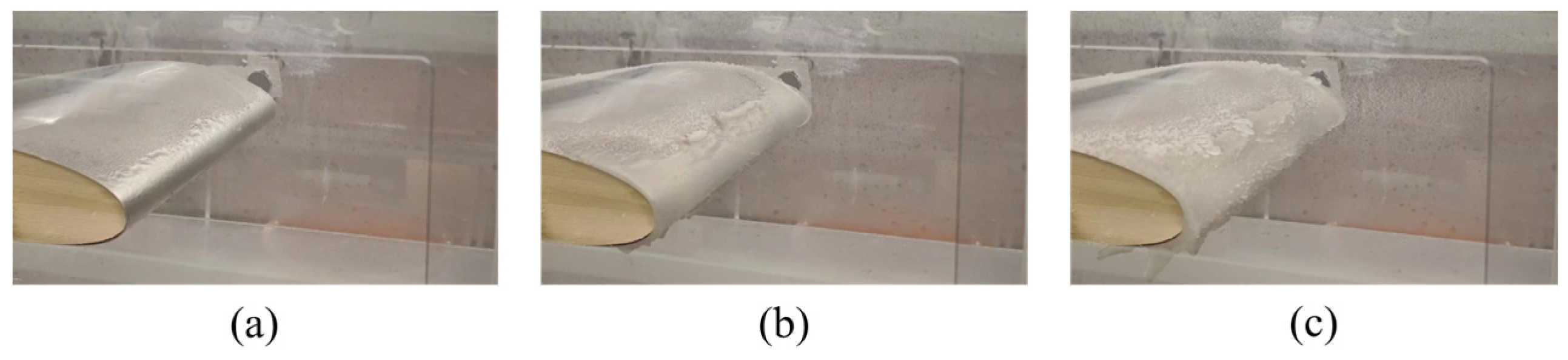
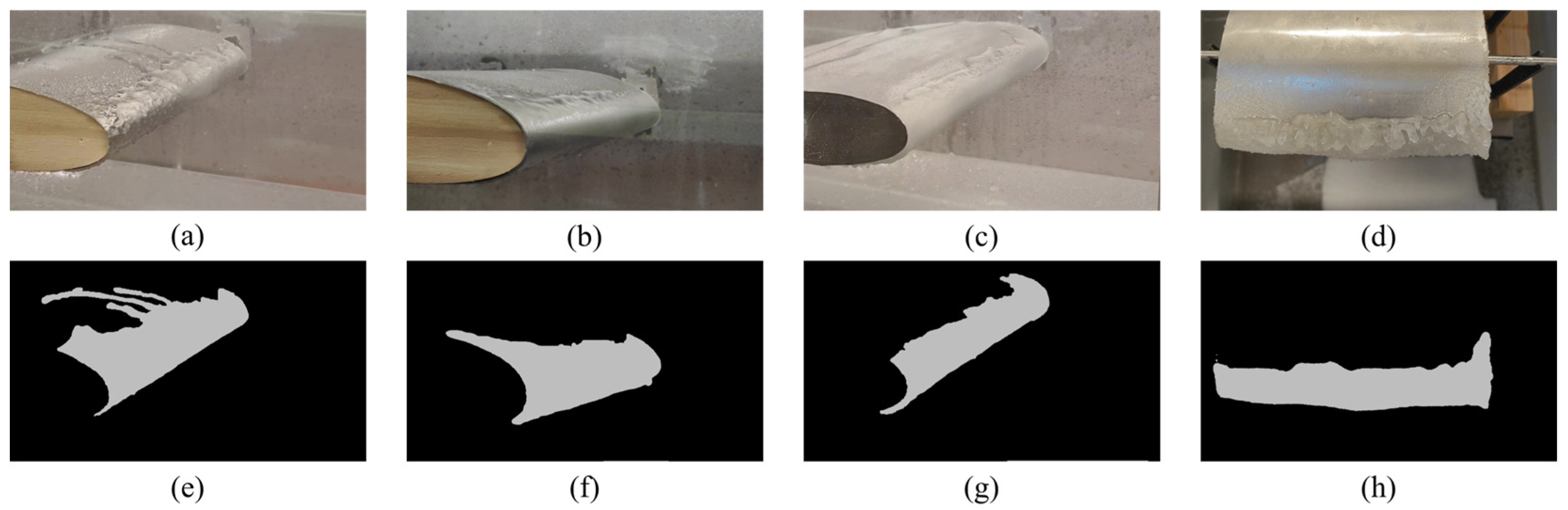
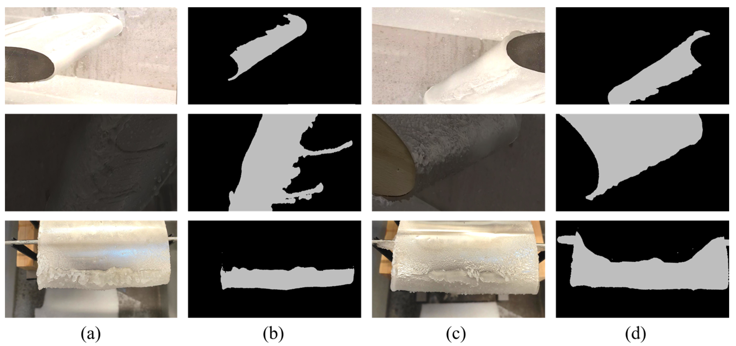
2.1. Image Data Acquisition Annotation

No publicly available dataset exists for wing icing, and relevant research in this area has certain limitations. To address this gap, this study utilizes a small desktop recirculating icing wind tunnel (see Figure 1) to conduct wing icing experiments under natural light. Various wing types are tested under different icing conditions. Given that icing formation varies with environmental factors, the angle of attack and ambient temperature are selected as key experimental variables to ensure the uniqueness of each test. The measurement of certain parameters in the experimental ice wind tunnel is detailed in Appendix A.
Image data acquisition is performed using a Xiaomi smartphone, which captures videos of the icing process. A fixed tripod is positioned 10 cm to 30 cm from the experimental section to ensure consistent framing. Each icing experiment lasts five minutes, allowing for the transition from an initial clear ice state to a significantly iced condition. The specific experimental setup is detailed in Table 1.
As the icing process progresses, the ice accumulation on the wing leading edge increases over time. Initially, icing forms on the leading edge, exhibiting high transparency, which may cause the model to misclassify ice as part of the wing, potentially limiting detection performance (see Figure 2a). As icing continues, the ice layer thickens near the leading edge, making the distinction between ice and wing more apparent (see Figure 2b). Eventually, the ice fully covers the leading-edge area (see Figure 2c). To develop a robust icing detection model capable of identifying different icing stages, the final dataset includes images representing all three icing states.
For video data processing, frames are extracted at three-second intervals, yielding 1300 original wing icing images. These images capture front and side views of ice accumulation within five minutes for each wing type. The dataset is manually labeled, categorizing images into ice and background classes (see Figure 3).

2.2. Data Augmentation

Data augmentation is a crucial technique in deep learning for enhancing dataset diversity. It is particularly beneficial for datasets with limited samples or suboptimal quality. Standard data augmentation methods include flipping, rotation, cropping, scaling, and translation.
Due to experimental constraints, the acquired icing images were captured from a single perspective under consistent lighting conditions. However, aircraft operate in diverse lighting environments, including low-light conditions. This study employs offline data augmentation to enhance the dataset and address this limitation. Five transformations—random flipping, random rotation, random scaling, brightness adjustment, and contrast adjustment—are applied to the icing images and their corresponding labels. These data augmentation operations expanded the dataset size and improved data quality, facilitating model convergence and generalization performance. Ultimately, 5000 processed images were obtained, with some samples shown in Figure 4. Each transformation is applied independently, ensuring uniqueness in the augmented dataset. The dataset is then partitioned into training, validation, and test sets, with 3000 images allocated for training and 1000 images each for validation and testing.

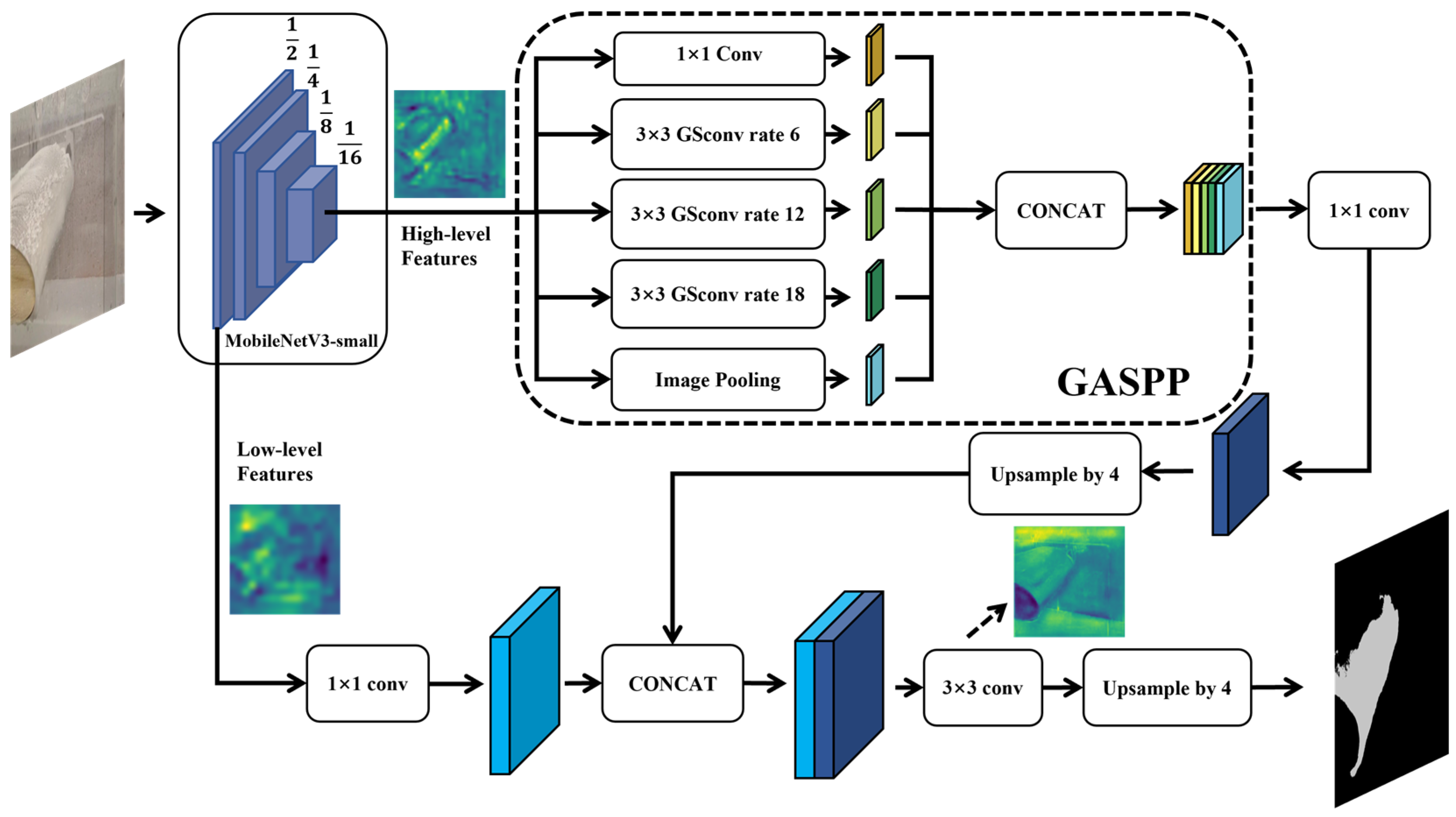
2.3. Improved DeeplabV3+ for the Leading Edge of Airfoil Icing Detection

The Deeplab [26] algorithm is a classic image segmentation algorithm capable of achieving high-precision image segmentation. As the latest network architecture in the Deeplab series, DeeplabV3+ delivers high-precision segmentation on most image segmentation datasets, surpassing the majority of known image segmentation algorithms. The DeeplabV3+ algorithm primarily consists of three components: the backbone network (Backbone), the Atrous Spatial Pyramid Pooling (ASPP) module, and the feature fusion module. DeeplabV3+ employs Xception [27] as its backbone network to enhance the model’s feature extraction capability for input images. The ASPP module mainly utilizes atrous convolutions with different dilation rates stacked into a pyramid structure to capture image features at varying receptive fields, followed by fusion to strengthen the model’s ability to extract local features. The feature fusion module combines shallow features from the backbone network with the output features of the ASPP module, enabling the model to focus on both shallow semantic information and deep feature information. This forms an Encode-Decode structure, allowing the model to retain more feature information during the up-sample process, thereby improving overall performance. Experimental results on detecting ice accumulation on the wing leading edge under natural light demonstrate that the DeeplabV3+ model with Xception as the backbone network can effectively identify ice-covered regions.
To address the challenges of high ice transparency and indistinct edges in wing ice images under natural lighting conditions, this study builds upon DeeplabV3+ by introducing MobileNetV3 [28] as the backbone network and optimizing the ASPP module with the Ghost Conv [29] structure. Combined with transfer learning, this approach constructs a model tailored for detecting ice accumulation on the wing leading edge under natural lighting, enhancing both the model’s operational speed and its ability to perform fine-grained segmentation of the ice edge.
The WID-DeeplabV3+ network framework is illustrated in Figure 5. The model initially utilizes a backbone network to extract features from the input wing icing images. The output of the backbone network is bifurcated into two components: one is a deep feature map with a resolution of 1/16 of the original image, which encompasses high-level semantic information and abstract features of the image, enabling it to capture the complex morphology and structural characteristics of wing icing; the other is a shallow feature map with a resolution of 1/2 of the original image, retaining rich detailed information and spatial location information, which assists in accurately identifying the specific location of icing regions on the wing. The deep feature map is then fed into the GASPP module, where the dilation rates are set to [6,12,18]. Multi-scale feature information aggregation is achieved through convolutional operations with varying dilation rates. This multi-scale feature extraction method effectively captures the feature information of wing icing regions across different scales, whether it be fine textures or large-scale icing areas, ensuring precise extraction. The aggregated feature map is subsequently upsampled to match the size of the shallow feature map and concatenated with it. This fusion technique allows high-level semantic information and low-level detailed information to complement each other, constructing a more comprehensive and discriminative feature representation. Subsequently, two convolutional layers are employed to aggregate the features as the model output. The specific details of the WID-DeeplabV3+ model will be elaborated in subsequent chapters.

2.3.1. MobileNetV3 as Backbone

The Google research team proposed MobileNetV3 in 2019. As the third-generation lightweight network in the MobileNet series, this architecture is specifically designed for mobile and embedded devices, reducing computational complexity and parameter count while maintaining high accuracy, thereby improving inference speed. As an enhanced version of MobileNetV2 [30], MobileNetV3 retains the lightweight characteristics of its predecessor while achieving higher efficiency and accuracy through multiple innovations and optimizations.
MobileNetV3 employs advanced depthwise separable convolution technology, significantly reducing computational costs and parameter numbers compared to standard convolutions, making it particularly suitable for resource-constrained devices. In terms of architectural design, the network introduces a novel activation function called h-swish, which improves model accuracy while maintaining computational efficiency. Compared to the ReLU6 activation function used in MobileNetV2, h-swish performs better in low-precision environments, enhancing the network’s expressive capability. MobileNetV3 utilizes Neural Architecture Search (NAS) technology to automatically determine the optimal network configuration, maximizing recognition accuracy while minimizing model size and computational load. The network also optimizes inter-layer connections and incorporates the Squeeze-and-Excitation (SE) attention mechanism, adaptively adjusting feature map weights to focus on key feature information, further improving feature extraction capability. The basic structure of MobileNetV3 is shown in Figure 6.
The detailed settings are consistent with those described in the MobileNetV3 paper. Initially, a 1 × 1 convolution operation is used to expand the channel dimensions of the initial input feature map, enriching the feature information for subsequent operations without significantly increasing computational costs. This is followed by a 3 × 3 depthwise convolution, which performs independent convolution operations on each input channel to achieve effective spatial information interaction and extract local image features. Subsequently, the SE attention mechanism is applied to adaptively adjust the feature maps output by the depthwise convolution across channels. This mechanism compresses the spatial dimensions via global average pooling, then learns channel weights through two fully connected layers, and finally reweights the feature maps based on these weights, significantly enhancing the expressive power of key features. Lastly, a 1 × 1 convolution is used to fuse information along the channel dimensions, adjusting the feature maps to the appropriate size. Through residual connections, this output is added to the result of the initial 1 × 1 convolution in the module, mitigating gradient vanishing issues while enabling cross-layer feature reuse. The resulting processed feature map from the basic module serves as high-quality input for subsequent network layers.
In this study, the convolutional results before the last fully connected layer in the original MobileNetV3 network are used as the output feature maps for the WID-DeeplabV3+ backbone network. The intermediate layer outputs of MobileNetV3, with feature maps at one-quarter the size of the input image, serve as shallow features for subsequent feature fusion in WID-DeeplabV3+. Comparative experiments were conducted with other backbone networks. Table 2 presents the experimental results of leading-edge wing icing detection using different feature extraction networks (HrNetV2 [31], ResNet50 [32], Xception, and MobileNet) as backbone architectures. Among them, the DeeplabV3+ model with MobileNetV3 as the backbone network demonstrates advantages in detection performance and parameter count compared to other backbone networks. Specifically, using MobileNetV3 as the backbone network for the DeeplabV3+ model achieves the best detection performance with 2.33 M parameters and 12.07 G FLOPs computational load. Compared to other backbone networks, accuracy improves by 0.24–5.69%, IOU by 0.44–3.44%, precision by 0.15–4.85%, recall by 0.33–4.93% and dice by 0.24–4.89%. These results indicate that using MobileNetV3 as the backbone network significantly enhances the model’s runtime speed and certain detection performance metrics.

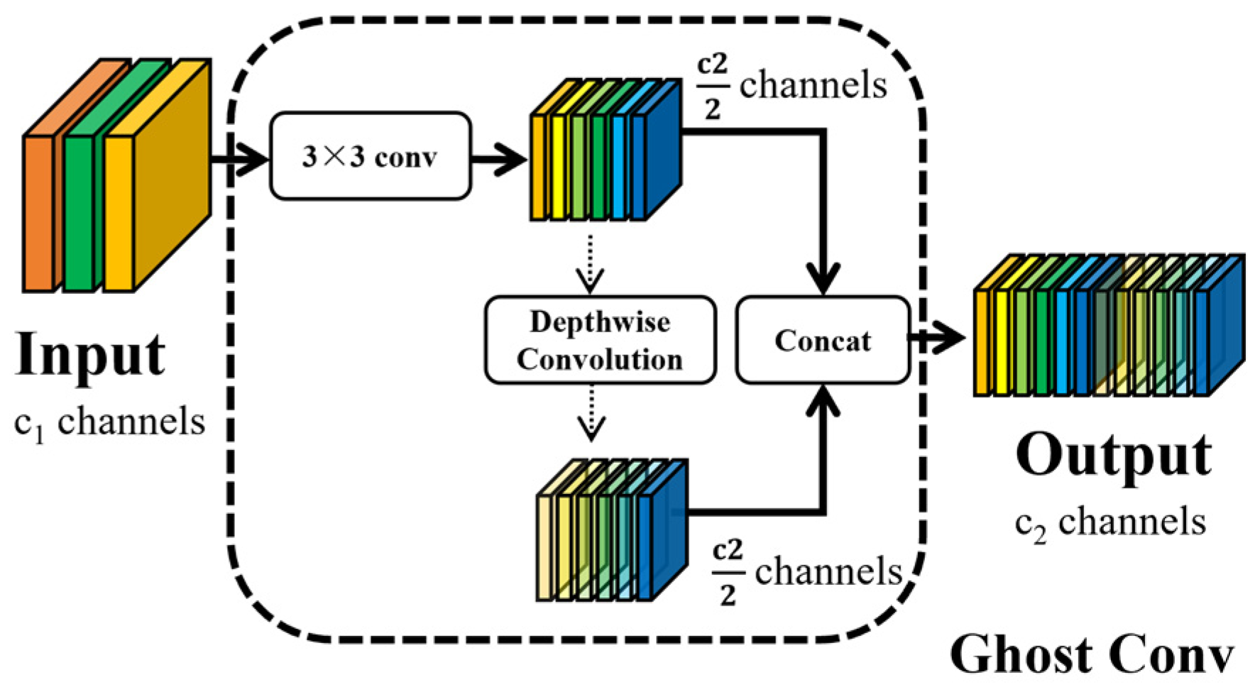
2.3.2. Ghost Atrous Spatial Pyramid Pooling Module

In the video sequence, the wing icing area undergoes a dynamic evolution process, expanding from small to large and from thin to thick, and it occupies only a partial region of the image. The original DeepLabV3+ algorithm utilizes the ASPP module, which extracts features from the input feature map using convolutional kernels with different dilation rates. By employing dilated convolutions with varying receptive fields, the ASPP module captures long-range dependencies and enhances multi-scale contextual information, thereby improving the feature extraction capability.
However, achieving a sufficiently large receptive field requires setting high dilation rates, which significantly increases computational complexity and the number of parameters. The original ASPP module suffers from excessive computational overhead, negatively impacting the model’s inference speed. Moreover, an excessively large receptive field may cause the model to overly focus on large-scale icing areas while neglecting the fine-grained features of small-scale icing regions, thereby reducing segmentation accuracy in these areas.
To address these limitations, this study proposes a GASPP module that integrates GSConv (see Figure 7) with ASPP. The input feature map is processed using a standard 3 × 3 convolutional layer to generate an intermediate feature map with half the number of target channels. Subsequently, a 3 × 3 depthwise convolution is applied to this intermediate feature map, where the depthwise convolution operation performs independent convolution calculations within each channel, thereby producing a Ghost feature map with the same number of channels as the intermediate feature map. Finally, the intermediate feature map and the Ghost feature map are concatenated along the channel dimension, resulting in a new feature map that serves as the final output of this module. This structural design effectively reduces computational complexity and parameter count while maintaining strong feature representation capabilities.
To mitigate the high computational cost and parameter count of the original ASPP module, we introduce the GASPP module that replaces standard convolutions with Ghost convolutions. This technique generates additional feature maps using fewer parameters while maintaining the same output dimensions. Specifically, GSConv enhances model accuracy by preserving hidden inter-channel connections while maintaining low time complexity, achieving a balance between information loss from standard convolutions and depthwise separable convolutions. Furthermore, this method effectively reduces the network’s parameter count and computational complexity. When the feature map size is H × W with C channels and the output channel is N, the computational cost ratio (1) and parameter count ratio (2) between standard convolution and Ghost Conv are as follows:
r s = N H W C k k N s H W C k k + ( s 1 ) N s H W C d d = C k k 1 s C k k + ( s 1 ) s C d d s C s + C 1 s
r s = N C k k N s C k k + ( s 1 ) N s d d s C s + C 1 s
Among them, k refers to the convolution kernel size; d is the convolution kernel size during linear operations, similar to k; and s denotes the number of linear transformations, with s << c.
In this study, the s value in the GASPP module is set to 2. By integrating GSConv into the ASPP structure, this research replaces some conventional convolutions, ultimately constructing the GASPP module. While maintaining the same dilation rates [6,12,18] as ASPP, GASPP significantly improves the model’s inference speed.

2.4. Evaluation Standard

This study employs metrics including accuracy, intersection over union (IOU), precision, recall, dice, parameter, computational complexity, and inference time to comprehensively evaluate the model’s performance in wing ice detection. In image segmentation tasks, the relationship between predicted pixel categories and their corresponding annotations can be classified into four types: True Positive (TP)—pixels correctly classified as positive samples; False Negative (FN)—pixels that should have been classified as positive but were incorrectly identified as negative; False Positive (FP)—pixels that should have been classified as negative but were incorrectly identified as positive; and True Negative (TN)—pixels correctly classified as negative samples. Accuracy is defined as the ratio of correctly predicted samples to the total number of predictions, with the calculation formula provided in Equation (3). For segmentation tasks, IOU measures the ratio of the intersection area to the union area between predicted and annotated regions, where values closer to 1 indicate superior segmentation performance, as defined in Equation (4). Precision represents the proportion of correct predictions among all positive predictions, calculated according to Equation (5). Recall reflects the proportion of actual positive samples that were correctly predicted, calculated following Equation (6). The Dice coefficient is a similarity measure function between the true sample set and the predicted sample set, commonly used to represent the similarity between two samples. Its calculation follows Equation (7). Additionally, parameter count, computational complexity, and FPS are used to quantify model scale and inference speed.
A c c u r a c y = T P + T N T P + T N + F P + F N
I O U = T P T P + F P + F N
P r e c i s i o n = T P T P + F P
R e c a l l = T P T P + F N
D i c e = 2 T P 2 T P + F N + F P

3. Experimental Result and Analysis

3.1. Experimental Platform and Parameter Settings

All experiments were conducted on the Windows operating system using the PyTorch framework. The specific hardware configurations are detailed in Table 3. The model training employed a cross-entropy loss function [33] to calculate the difference between predicted values and ground truth, as defined in Equation (8):
L o s s = 1 N i = 1 N y i log ( p ( y i ) ) + ( 1 y i ) log ( 1 p ( y i ) )
Here, y represents a binary label, which can be either 0 or 1, and p(y) denotes the probability that the output corresponds to label y. The Adam [34] optimizer is utilized for optimization purposes, with an initial learning rate set at 0.001. Throughout the training process, a polynomial decay strategy is implemented to dynamically adjust the learning rate. To prevent overfitting, an L2 regularization technique with a coefficient of 0.0001 is applied.

3.2. Comparisons of Effects Before and After Improvement of the Model

Figure 8 illustrates the confusion matrices [35] and training loss curves for both the Deeplabv3+ and WID-DeeplabV3+ models. The DeeplabV3+ model frequently misclassified ice as background and vice versa, more so than the WID-DeeplabV3+ model. Moreover, the number of correctly identified background and ice instances was notably lower for the DeeplabV3+ model compared to the WID-DeeplabV3+ model. This suggests that the enhanced method improves the model’s ability to detect icing regions and decreases misclassification errors.
Table 4 provides a comparison of the accuracy, IOU, precision, recall, and dice for wing icing detection between the DeeplabV3+ and WID-DeeplabV3+ models under natural light. The findings indicate that the WID-DeeplabV3+ model significantly surpasses the DeeplabV3+ model in wing icing detection tasks: Accuracy of ice region detection increased by 1.83%, IOU values rose by 3.55%, precision improved by 1.79%, recall went up by 2.04% and dice improved by 1.92%. Furthermore, when handling input images at a resolution of 1920 × 1080, the WID-DeeplabV3+ model sustains a consistent detection speed of 0.03 s, fulfilling real-time detection requirements. In summary, the WID-DeeplabV3+ model effectively and accurately completes the task of detecting leading-edge wing icing in natural lighting conditions.

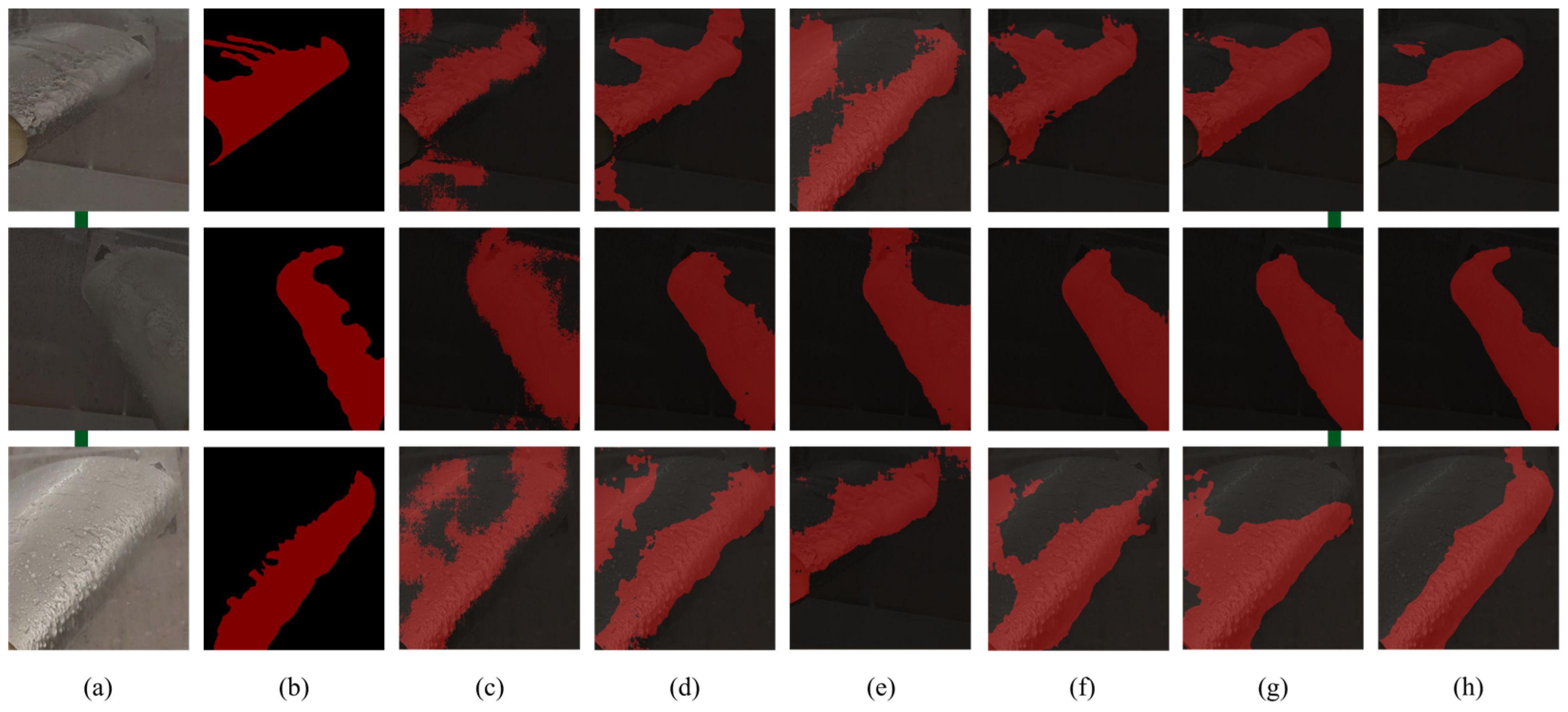
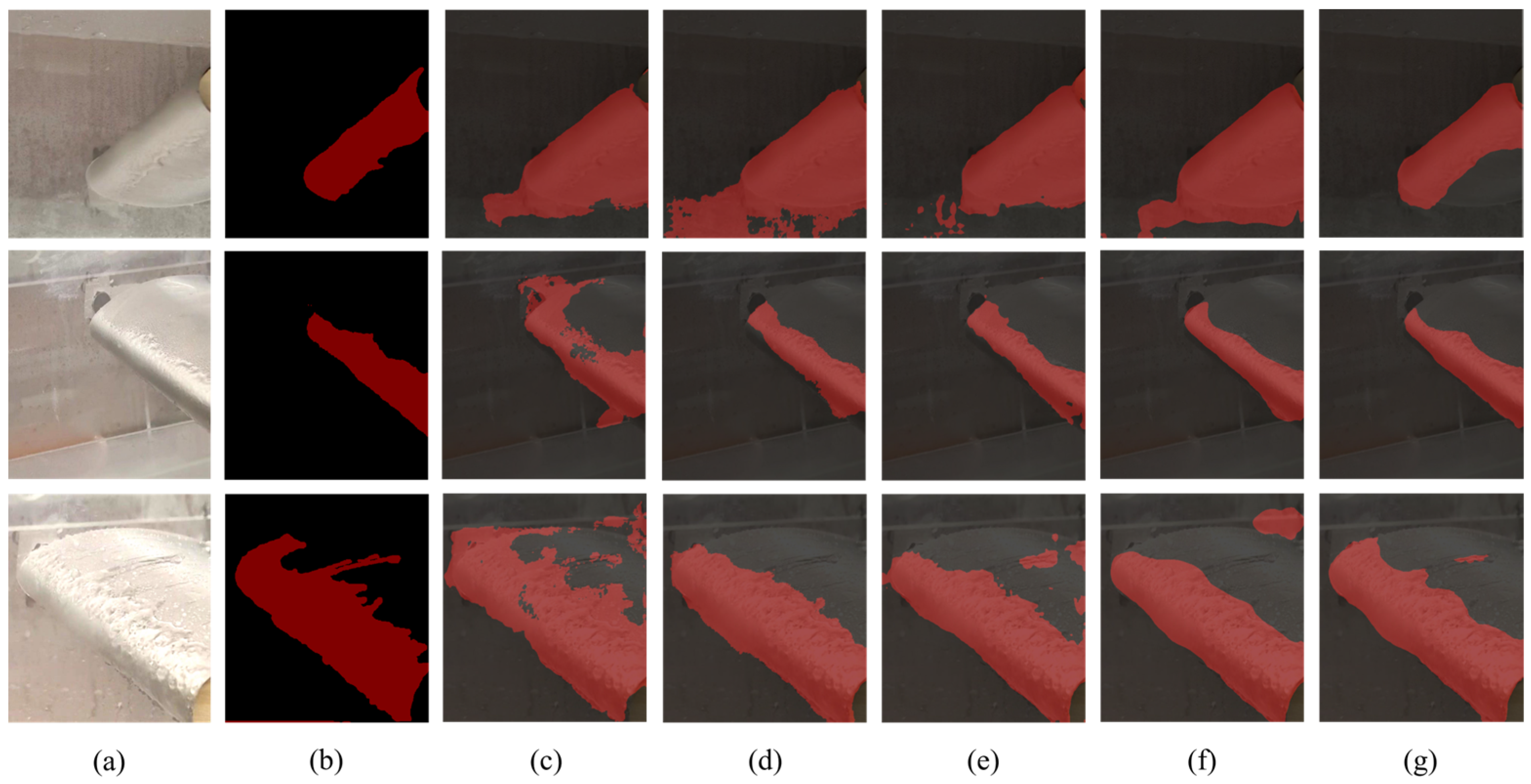
3.3. Comparison Experiments of Different Models

To further validate the performance of the improved model, we conducted verification tests on the same dataset. The WID-DeeplabV3+ model was compared with multiple mainstream image segmentation models, including FCN [36], SegNet [37], UNet [38], UNext [39], PSPNet [40], BiSeNet [41], ENet [42], DABNet [43], and DeeplabV3+. Table 5 presents the performance metrics of each detection algorithm, while Figure 9 shows the comparison of some detection results.
The data in Table 5 indicate that at the same training conditions, WID-DeeplabV3+ outperforms other models in terms of accuracy, IOU, precision, recall, and dice. Although it does not have the smallest number of parameters or computational load, when considering both detection accuracy and model runtime speed, WID-DeeplabV3+ demonstrates the best overall performance among the aforementioned image segmentation models, achieving a better balance between detection accuracy and speed. Specifically, compared to other models, WID-DeeplabV3+ improves accuracy by 1.87–10.26%, IOU by 3.55–18.26%, precision by 1.79–11.52%, recall by 2.04–10.96% and dice by 1.92–10.75%.
As shown in Figure 10 and Figure 11, we compared the wing icing region detection performance of different models. Figure 10h and Figure 11g demonstrate that the proposed model accurately segments the boundaries of icing regions, reducing missed and false detections while improving the wing icing regions detection accuracy. These visualization results of leading-edge wing icing confirm that by adopting MobileNetV3 as the backbone network, combined with the GASPP module and transfer learning, the model achieves higher accuracy in wing icing detection tasks. Its segmentation accuracy significantly surpasses other comparative models, with improved handling of missed and false detections, finer segmentation of icing region edges, efficient operation with fewer parameters, and lower computational costs.

3.4. Network Improvement Ablation Experiments

Ablation experiments are typically employed in complex neural networks to investigate the influence of specific substructures, training strategies, and hyperparameters on model performance, playing a crucial guiding role in neural network architecture design. To evaluate the effectiveness of the proposed improvements, this study systematically assesses model performance through ablation experiments. By incrementally adding modules to the baseline model, the contribution of each component is analyzed. All experiments are conducted under identical conditions to ensure consistency in hyperparameter configuration.
To validate the efficacy of MobileNetV3 as the backbone network, the GASPP module, and the transfer learning method, ablation experiments were performed as shown in Table 6. The results demonstrate that adopting MobileNetV3 as the backbone of DeepLabV3+ achieves a balance between accuracy and computational efficiency in aircraft wing leading edge icing detection tasks. Compared to the original DeepLabV3+ backbone network Xception, the MobileNetV3-based DeepLabV3+ model reduces parameters by 93% and computational cost by 76%, with slight improvements in other metrics.
After incorporating the GASPP module, the model parameters and computational load further decrease while performance slightly improves. By employing transfer learning—initializing the weights of WID-DeepLabV3+ with the pre-trained MobileNetV3 weights from the ImageNet dataset [44]—the accuracy, IOU, precision, and recall increase by 1.83%, 3.55%, 1.79%, and 2.04%, respectively, while model parameters and computational requirements significantly decrease.
To comprehensively evaluate the detection performance of the WID-DeeplabV3+ model on wing icing regions, Figure 12 presents the heatmap visualization results generated by Gradient-weighted Class Activation Mapping (Grad-CAM) for both DeeplabV3+ and WID-DeeplabV3+, illustrating the visual representation of wing icing region detection. All images in Figure 8 are sourced from the test set of the wing icing dataset, including images with thin icing, thick icing, and those captured from varying perspectives. It is important to note that warmer colors in the heatmaps indicate higher contribution of the corresponding regions to the icing detection results, signifying greater model attention to those areas.
As shown in Figure 12c,f,i, when the DeeplabV3+ model is employed for wing icing region detection, it is prone to interference from small water droplets or ice beads condensed on the wing surface, as well as the wing skin, leading to reduced attention on the leading-edge icing regions. This is the primary reason why the model often exhibits missed detections, false detections, and insufficient edge detection precision during wing icing detection. However, after optimization, the heatmaps of WID-DeeplabV3+ (Figure 12b,e,h) demonstrate significantly enhanced focus on the leading-edge icing regions while effectively suppressing attention to irrelevant background areas. This observation confirms the efficacy of the optimization—WID-DeeplabV3+ strengthens attention to wing icing regions while mitigating background interference.
The experimental results indicate that these optimizations enable the model to more effectively utilize contextual information, thereby improving focus on icing regions while reducing interference from irrelevant backgrounds. The heatmap visualization ultimately proves that these enhancements significantly improve the model’s performance in detecting leading-edge wing icing regions under natural lighting conditions.

4. Discussion

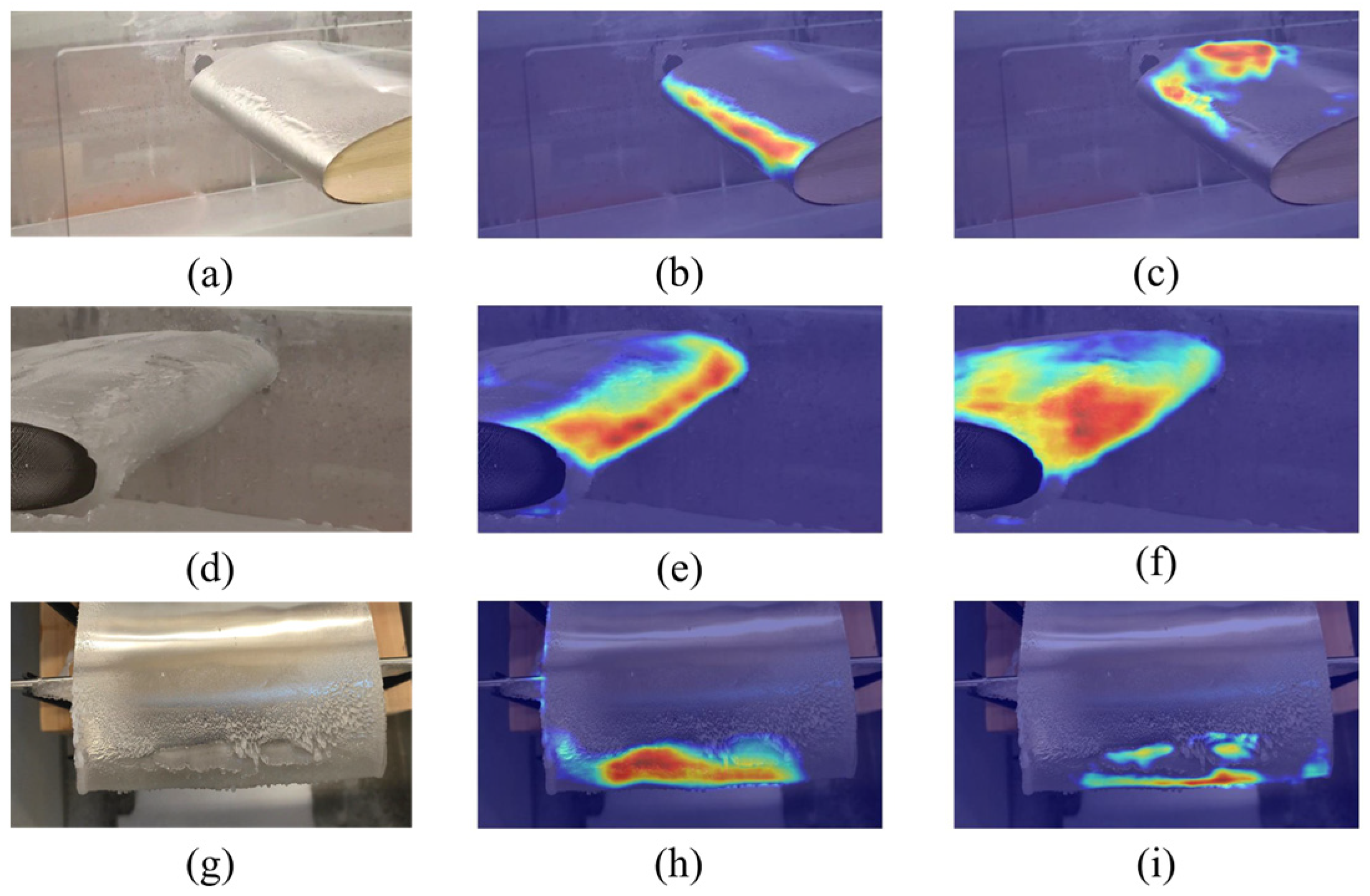
4.1. Feasibility Analysis of Wing Leading Edge Icing Detection Under Natural Lighting Conditions

When ice initially forms on the wing, the accumulation is thin. Due to the high transparency of ice, the model may exhibit low sensitivity to the characteristics of ice during this early stage, leading to misclassification—either identifying clean wings as iced or failing to detect actual ice formation, resulting in missed or false detections. To further evaluate the performance of the WID-DeeplabV3+ model in detecting early-stage ice accretion on wing leading edge under natural light, the research team conducted supplementary experiments to analyze the initial ice formation. The heatmaps of the original model and WID-DeeplabV3+ are shown in Figure 13.
Figure 13a displays images extracted at 5-frame intervals from a video of wing leading edge ice accretion, covering five sequential stages from no ice to initial ice formation, demonstrating temporal correlation. The first and second images show no ice, while the third to fifth exhibit ice formation. Figure 13b presents the heatmap visualization results of the original model, which shows high attention on clean wing areas, increasing the likelihood of false detections. As ice begins to form on the leading edge, DeeplabV3+ does not distinctly shift its focus to the iced regions, maintaining significant attention on non-iced areas. Figure 13c illustrates the heatmap visualization of the WID-DeeplabV3+ model. For ice-free images, the model still focuses on the wing surface but shows marked improvement compared to DeeplabV3+. As ice forms on the leading edge, WID-DeeplabV3+ progressively concentrates its attention on the iced regions and stabilizes over time, indicating that the model has better learned the features of ice accretion and demonstrates superior detection capabilities.
These results demonstrate that the WID-DeeplabV3+ model exhibits stronger feature extraction for early-stage ice formation on the wing leading edge under natural light, with significantly improved detection performance over the original model. Thus, it is expected to deliver superior detection performance in practical applications.

4.2. Limitations of the WID-DeeplabV3+ Model

It should be specifically noted that during actual aircraft flight, the wing icing environment is extremely complex and subject to numerous interference factors. The dataset collected in this experiment was obtained through tests conducted in an icing wind tunnel, which may exhibit certain discrepancies from real-world conditions. Due to the limitations of the data acquisition equipment and icing wind tunnel facilities, this study did not account for the special scenario of direct sunlight exposure on the camera lens, focusing instead on airflow variations during flight, changes in lighting, high transparency of ice accumulation, and the indistinct edge of icing regions. Consequently, the model’s detection performance may be constrained under extremely low-light conditions or when light directly strikes the camera lens. Additionally, during the initial stages of wing icing, the ice layer is extremely thin and may reflect the wing’s inherent color, potentially leading to false or missed detections by the model. Therefore, future efforts will involve collecting a substantial volume of images featuring extreme scenarios and early-stage thin ice accumulation as new data, combined with post-processing techniques to achieve precise detection of icing regions on the wing leading edge, thereby enhancing the model’s capability to detect extreme scenarios and early-stage icing.

5. Conclusions

Ice detection is a critical measure for aircraft to address icing interference during flight, ensuring flight safety to a certain extent. To rapidly remove ice accumulation on the leading edge of wings and minimize its impact on wing performance, it is essential to detect leading-edge ice conditions quickly and accurately. This study conducts an in-depth analysis of the technical challenges in detecting ice accumulation using leading-edge wing images and develops an innovative solution named “WID-DeeplabV3+.” The proposed method incorporates the MobileNetV3 network and introduces the GASPP module, enabling effective detection of leading-edge ice accumulation, precise segmentation of ice region edges, and improved model runtime efficiency. Specifically, our approach achieves accuracy of 97.15%, intersection over union (IOU) of 94.16%, recall of 97%, precision of 96.96% and dice of 96.98%. These positive results validate the feasibility of the proposed method for detecting leading-edge ice accumulation on aircraft wings under natural lighting conditions, while also indicating the need for continued optimization and exploration. The proposed model demonstrates robust detection performance across thin to thick ice accumulation stages on the wing leading edge, making it suitable for real-time monitoring and serving as an auxiliary tool for de-icing tasks. Future plans include constructing a multi-task dataset (e.g., more diverse wing types, real-world wing icing images, and ice accumulation under other light sources) to develop a detection system that mitigates the interference of external lighting conditions on airfoil leading edge icing detection performance. Although the model is specifically designed for the wing leading edge, it can be extended to detect ice accumulation on other parts of the aircraft. Through ongoing research, this work will provide more valuable technical options for detecting ice accumulation during aircraft flights.

Author Contributions

Y.Y.; Writing—original draft, Investigation, Visualization, Validation, Software, Methodology, Formal analysis, Conceptualization, Data curation. C.T.; Writing—review and editing, Investigation, Formal analysis, Data curation, Software. J.H.; Data curation, Validation. Z.C.; Data curation, Visualization. Z.X.; Funding acquisition, Project administration, Resources, Writing—review and editing. All authors have read and agreed to the published version of the manuscript.

Funding

This work is supported by the Shenzhen Science and Technology Program (JCYJ20220530145203007).

Data Availability Statement

The raw data supporting the conclusions of this article will be made available by the authors on request.

Acknowledgments

We would like to thank the anonymous reviewers for their valuable suggestions.

Conflicts of Interest

The authors declare no conflicts of interest.

Appendix A

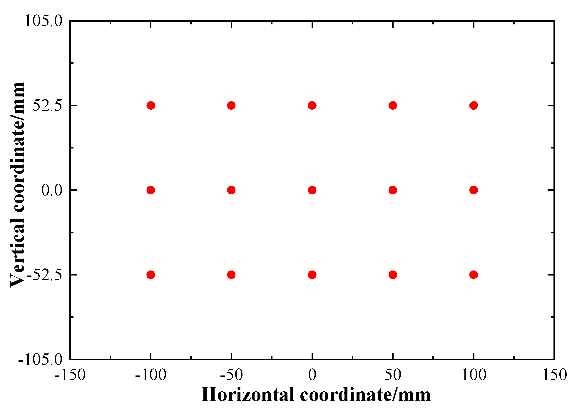
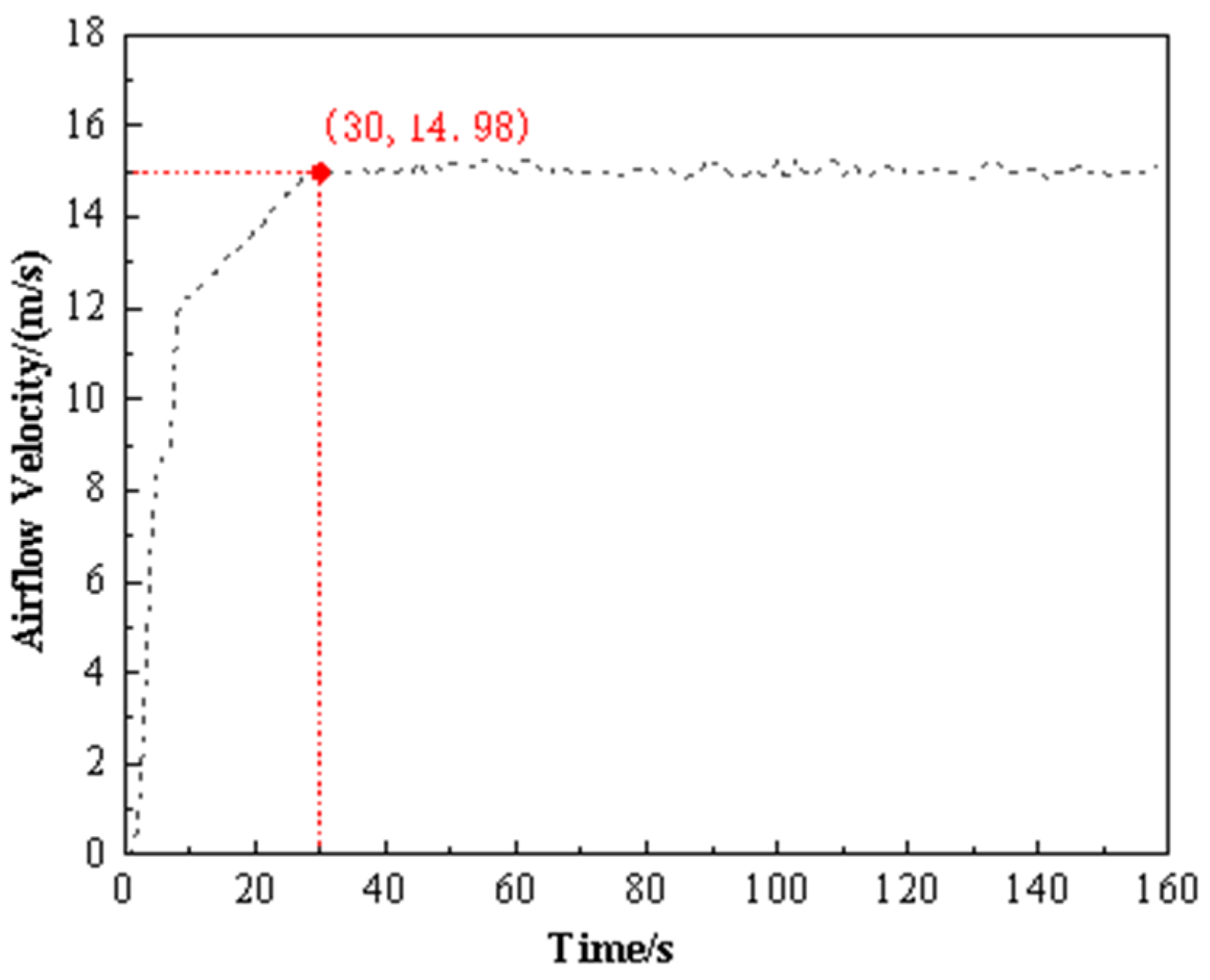
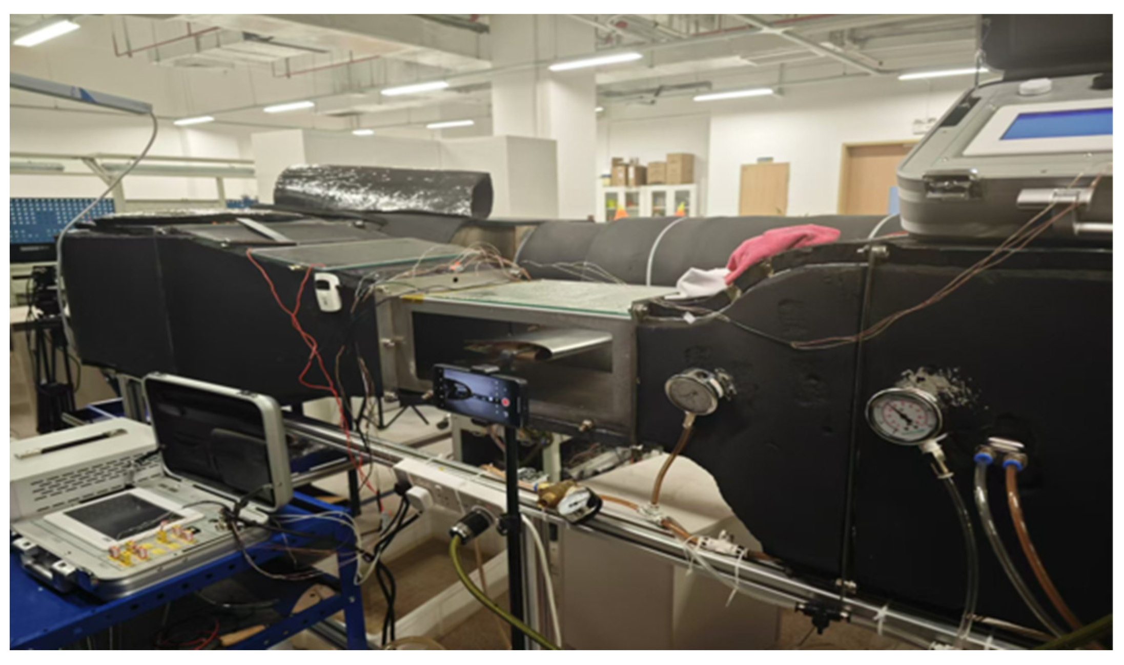
Appendix A.1. The Wind Speed and Wind Speed Uniformity Test

The uniformity of wind speed distribution within the test section indicates the quality of the flow field. A Testo 405i hot-wire anemometer was utilized to measure the wind speed in the test section, boasting a measurement accuracy of ±0.3 m/s. Throughout the measurement process, all axial fans were initially operated at full power to document the wind speed variation curve at the central position of the test section. Following this, the wind speed was regulated to 5 m/s and 15 m/s, respectively, to record the wind speed values at all locations specified in Figure A1. The final test results are presented in Figure A2 and Figure A3. The wind speed increase curve for the ice wind tunnel test section is depicted in Figure A2. Figure A3 illustrates the wind speed distribution across the test section’s cross-section at wind speeds of 5 m/s and 15 m/s, respectively.
Figure A1. Location of measurement points in the test section.
Aerospace 12 00627 g0a1
Figure A2. Airflow velocity increase curve in the test section.
Aerospace 12 00627 g0a2
Figure A3. Airflow velocity distribution in the test section under different wind speeds.
Aerospace 12 00627 g0a3

Appendix A.2. The Minimum Temperature and Temperature Uniformity Test

During the temperature testing, the power and refrigeration systems were activated, with the airflow velocity maintained at 10 m/s. The chiller shutdown temperature was set to −30 °C. The temperature variation at the center of the test section was continuously recorded using a thermocouple. In addition, the temperature readings from all thermocouples were recorded at two target temperatures: −5 °C and −15 °C. The cooling curve of the ice wind tunnel test section is depicted in Figure A4. Figure A5 displays the final outcomes of the experimental tests.
Figure A4. Cooling curve of the test section.
Aerospace 12 00627 g0a4
Figure A5. Temperature distribution in the test section at different temperatures.
Aerospace 12 00627 g0a5

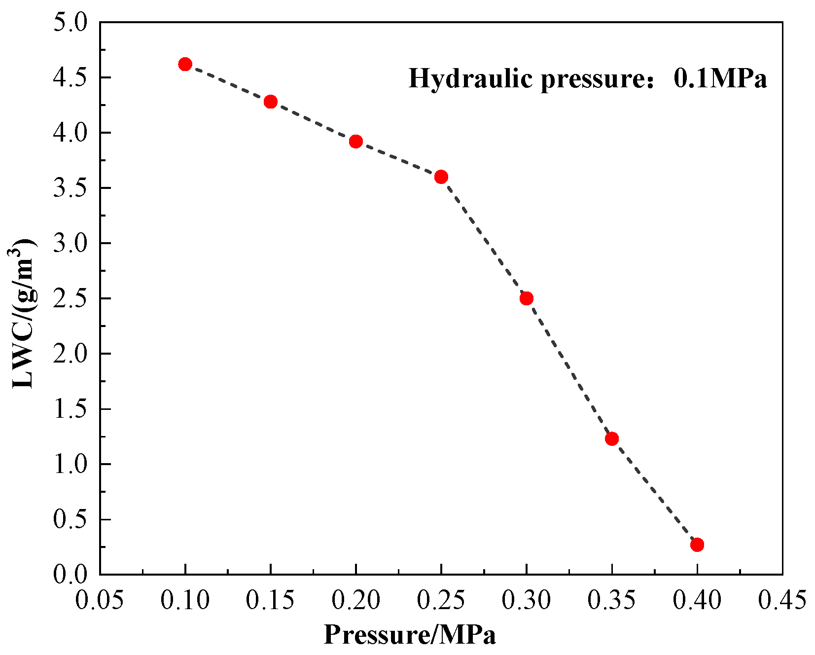
Appendix A.3. The MVD and LWC Test

The MVD was measured using a machine vision method. Spray images were captured using a high-intensity light source in combination with a FLIR industrial camera. After pixel calibration, droplet contours were identified using OpenCV, and the volumetric distribution was subsequently calculated. As shown in Figure A6, when the liquid pressure was maintained at 0.1 MPa, the MVD decreased with increasing air pressure, ranging from 12.68 μm to 25.04 μm.
Figure A6. The variation of MVD with air pressure.
Aerospace 12 00627 g0a6
The LWC was measured using an improved multi-row ice accretion probe method. Five rows of ice accretion blades were evenly distributed across the test section. After 60 s of spray operation, the ice thickness at various heights along each blade was measured using a vernier caliper. The LWC was calculated according to the standard formula. The LWC at each measurement point was ultimately calculated using Formula (A1).
L W C = ρ i c e Δ S E b v t
In the equation, ρice is the density of ice, ∆S is the ice accretion thickness, Eb is the collection coefficient, v is the wind speed in the test section, and t is the collection time. Figure A7 indicates that under a constant liquid pressure of 0.1 MPa, the LWC decreases linearly with increasing air pressure, ranging from 0.27 to 4.62 g/m3.
Figure A7. The variation of LWC with air pressure.
Aerospace 12 00627 g0a7

References

  1. Yi, X.; Gui, Y.; Zhu, G.; Du, Y. Experimental and computational investigation into ice accretion on airfoil of a transport aircraft. J. Aerosp. Power 2011, 26, 808–813. [Google Scholar] [CrossRef]
  2. Mason, B.J. Physics of Clouds and Precipitation. Nature 1954, 174, 957–959. [Google Scholar] [CrossRef]
  3. Wang, H.; Huang, X.; Zhang, B. Design Theory of Vibrating-tube Ice Detector. Instrum. Tech. Sens. 2008, 3, 9–11. [Google Scholar] [CrossRef]
  4. Wei, L.; Jie, Z.; Lin, Y. A Fiber-Optic Aircraft Icing Detection System Using Double Optical Paths Based on the Theory of Information Fusion. Chin. J. Sens. Actuators 2009, 22, 1352–1355. [Google Scholar] [CrossRef]
  5. Zhou, J. Aircraft Icing Type Detection Based on Oblique End-face Fiber Optic Technology. Master’s Thesis, Huazhong University of Science and Technology, Wuhan, China, 2014. [Google Scholar] [CrossRef]
  6. Cheng, P.; Wu, C. Neural network based robust adaptive nonlinear control for aircraft under one side of wing loss. Syst. Eng. Electron. 2016, 38, 607–617. [Google Scholar]
  7. Yi, X.; Zhu, G.; Wang, K.; Li, S. Numerically simulating of ice accretion on airfoil. Acta Aerodyn. Sin. 2002, 20, 428–433. [Google Scholar] [CrossRef]
  8. Yi, X.; Wang, K.; Ma, H.; Zhu, G. 3-D numerical simulation of droplet collection efficiency in large-scale wind turbine icing. Acta Aerodyn. Sin. 2013, 31, 745–751. [Google Scholar]
  9. Gui, X.; Zeng, F.; Gao, J.; Fu, X.; Li, Z. Detection of Aircraft wing icing and de-icing by optical fiber sensing with FBG array. Measurement 2025, 247, 116748. [Google Scholar] [CrossRef]
  10. Zheng, D.; Li, Z.; Du, Z.; Ma, Y.; Zhang, L.; Du, C.; Li, Z.; Cui, L.; Xuan, X.; Deng, X. Design of capacitance and impedance dual-parameters planar electrode sensor for thin ice detection of aircraft wings. IEEE Sens. J. 2022, 22, 11006–11015. [Google Scholar] [CrossRef]
  11. Ikiades, A. Fiber optic ice sensor for measuring ice thickness, type and the freezing fraction on aircraft wings. Aerospace 2022, 10, 31. [Google Scholar] [CrossRef]
  12. Ding, L.; Yi, X.; Hu, Z.; Guo, X. Experimental Study on Optimum Design of Aircraft Icing Detection Based on Large-Scale Icing Wind Tunnel. Aerospace 2023, 10, 926. [Google Scholar] [CrossRef]
  13. Kim, Y.; Ye, B.-Y.; Suk, M.-K. AIDER: Aircraft Icing Potential Area DEtection in Real-Time Using 3-Dimensional Radar and Atmospheric Variables. Remote. Sens. 2024, 16, 1468. [Google Scholar] [CrossRef]
  14. Abdelghany, E.S.; Farghaly, M.B.; Almalki, M.M.; Sarhan, H.H.; Essa, M.E.-S.M. Machine learning and iot trends for intelligent prediction of aircraft wing anti-icing system temperature. Aerospace 2023, 10, 676. [Google Scholar] [CrossRef]
  15. Li, S.; Qin, J.; He, M.; Paoli, R. Fast evaluation of aircraft icing severity using machine learning based on XGBoost. Aerospace 2020, 7, 36. [Google Scholar] [CrossRef]
  16. Strijhak, S.; Ryazanov, D.; Koshelev, K.; Ivanov, A. Neural network prediction for ice shapes on airfoils using icefoam simulations. Aerospace 2022, 9, 96. [Google Scholar] [CrossRef]
  17. Hoover, G.A. Aircraft Ice Detectors and Related Technologies for Onground and Inflight Applications; Fedaral Aviation Administration Technical Center; Atlantic City International Airport: Atlantic County, NJ, USA, 1993; Volume 1993, p. 54. Available online: http://catalog.hathitrust.org/Record/102586835 (accessed on 1 April 1993).
  18. Ikiades, A.A.; Armstrong, D.J.; Hare, G.G.; Konstantaki, M.; Crossley, S.D.; Culshaw, B.; Marcus, M.A.; Dakin, J.P.; Knee, H.E. Fiber optic sensor technology for air conformal ice detection. Ind. Highw. Sens. Technol. 2004, 5272, 357–368. [Google Scholar] [CrossRef]
  19. Guo, L.; Qin, S.; Li, Q.; Liu, S.; Wang, Z. Research on ice contour extraction of aircraft model based on machine vision. Autom. Instrum. 2020, 6, 15–20. [Google Scholar]
  20. Qu, J.; Wang, Q.; Peng, B.; Yi, X. Icing prediction method for arbitrary symmetric airfoil using multimodal fusion. J. Aerosp. Power 2024, 39, 20220143. [Google Scholar] [CrossRef]
  21. Suo, W.; Sun, X.; Zhang, W.; Yi, X. Aircraft ice accretion prediction based on geometrical constraints enhancement neural networks. Int. J. Numer. Methods Heat Fluid Flow 2024, 34, 3542–3568. [Google Scholar] [CrossRef]
  22. Yu, D.; Han, Z.; Zhang, B.; Zhang, M.; Liu, H.; Chen, Y. A fused super-resolution network and a vision transformer for airfoil ice accretion image prediction. Aerosp. Sci. Technol. 2024, 144, 108811. [Google Scholar] [CrossRef]
  23. Zhang, D.; Wei, P.; Li, Q.; Tan, M. Novel Wing Icing Area Recognition Based on Morphological Processing Enhanced U-Net Network. In Proceedings of the 2021 IEEE 3rd International Conference on Civil Aviation Safety and Information Technology (ICCASIT), Changsha, China, 20–22 October 2021; pp. 1194–1997. [Google Scholar] [CrossRef]
  24. Su, X.; Guan, R.; Wang, Q.; Yuan, W.; Lyu, X.; He, Y. Ice area and thickness detection method based on deep learning. Acta Aeronaut. Astronaut. Sin. 2023, 44, 205–213. [Google Scholar] [CrossRef]
  25. Chen, L.-C.; Zhu, Y.; Papandreou, G.; Schroff, F.; Adam, H. Encoder-decoder with atrous separable convolution for semantic image segmentation. In Proceedings of the European Conference on Computer Vision (ECCV), Munich, Germany, 8–14 September 2018; pp. 801–818. [Google Scholar] [CrossRef]
  26. Chen, L.C.; Papandreou, G.; Kokkinos, I.; Murphy, K.; Yuille, A.L. Deeplab: Semantic image segmentation with deep convolutional nets, atrous convolution, and fully connected crfs. IEEE Trans. Pattern Anal. Mach. Intell. 2017, 40, 834–848. [Google Scholar] [CrossRef]
  27. Chollet, F. Xception: Deep learning with depthwise separable convolutions. In Proceedings of the IEEE Conference on Computer Vision and Pattern Recognition, Honolulu, HI, USA, 21–26 July 2017; pp. 1251–1258. [Google Scholar] [CrossRef]
  28. Howard, A.; Sandler, M.; Chen, B.; Wang, W.; Chu, G.; Chen, L.-C.; Chen, B.; Tan, M.; Vasudevan, V.; Zhu, Y.; et al. Searching for mobilenetv3. In Proceedings of the IEEE/CVF International Conference on Computer Vision, Seoul, Republic of Korea, 27 October–2 November 2019; pp. 1314–1324. [Google Scholar] [CrossRef]
  29. Han, K.; Wang, Y.; Tian, Q.; Guo, J.; Xu, C.; Xu, C. Ghostnet: More features from cheap operations. In Proceedings of the IEEE/CVF Conference on Computer Vision and Pattern Recognition, Seattle, WA, USA, 13–19 June 2020; pp. 1580–1589. [Google Scholar] [CrossRef]
  30. Sandler, M.; Howard, A.; Zhu, M.; Zhmoginov, A.; Chen, L.-C. Mobilenetv2: Inverted residuals and linear bottlenecks. In Proceedings of the IEEE Conference on Computer Vision and Pattern Recognition, Salt Lake City, UT, USA, 18–22 June 2018; pp. 4510–4520. [Google Scholar] [CrossRef]
  31. Sun, K.; Xiao, B.; Liu, D.; Wang, J. Deep high-resolution representation learning for human pose estimation. In Proceedings of the IEEE/CVF Conference on Computer Vision and Pattern Recognition, Long Beach, CA, USA, 15–20 June 2019; pp. 5693–5703. [Google Scholar] [CrossRef]
  32. He, K.; Zhang, X.; Ren, S.; Sun, J. Deep residual learning for image recognition. In Proceedings of the IEEE Conference on Computer Vision and Pattern Recognition, Las Vegas, NV, USA, 27–30 June 2016; pp. 770–778. [Google Scholar] [CrossRef]
  33. Ma, Y.; Liu, Q.; Qian, Z. Automated image segmentation using improved PCNN model based on cross-entropy. In Proceedings of the 2004 International Symposium on Intelligent Multimedia Video and Speech Processing, Hong Kong, China, 20–22 October 2004; pp. 743–746. [Google Scholar]
  34. Kingma, D.P. Adam: A method for stochastic optimization. In Proceedings of the International Conference for Learning Representations, San Diego, CA, USA, 7–9 May 2015. [Google Scholar] [CrossRef]
  35. Powers, D.M. Evaluation: From precision, recall and F-measure to ROC, informedness, markedness and correlation. Int. J. Mach. Learn. Technol. 2011, 2, 37–63. [Google Scholar] [CrossRef]
  36. Long, J.; Shelhamer, E.; Darrell, T. Fully convolutional networks for semantic segmentation. In Proceedings of the IEEE Conference on Computer Vision and Pattern Recognition, Boston, MA, USA, 7–12 June 2015; pp. 3431–3440. [Google Scholar] [CrossRef]
  37. Badrinarayanan, V.; Kendall, A.; Cipolla, R. Segnet: A deep convolutional encoder-decoder architecture for image segmentation. IEEE Trans. Pattern Anal. Mach. Intell. 2017, 39, 2481–2495. [Google Scholar] [CrossRef]
  38. Ronneberger, O.; Fischer, P.; Brox, T. U-net: Convolutional networks for biomedical image segmentation. In Proceedings of the Medical Image Computing and Computer-Assisted Intervention–MICCAI 2015: 18th International Conference, Munich, Germany, 5–9 October 2015; pp. 234–241. [Google Scholar] [CrossRef]
  39. Valanarasu, J.M.J.; Patel, V.M. Unext: Mlp-based rapid medical image segmentation network. In Proceedings of the International Conference on Medical Image Computing and Computer-Assisted Intervention, Singapore, 18–22 September 2022; pp. 23–33. [Google Scholar] [CrossRef]
  40. Zhao, H.; Shi, J.; Qi, X.; Wang, X.; Jia, J. Pyramid scene parsing network. In Proceedings of the IEEE Conference on Computer Vision and Pattern Recognition, Honolulu, HI, USA, 21–26 July 2017; pp. 2881–2890. [Google Scholar] [CrossRef]
  41. Yu, C.; Wang, J.; Peng, C.; Gao, C.; Yu, G.; Sang, N. Bisenet: Bilateral segmentation network for real-time semantic segmentation. In Proceedings of the European Conference on Computer Vision (ECCV), Malmö, Sweden, 8–13 September 2018; pp. 325–341. [Google Scholar] [CrossRef]
  42. Paszke, A.; Chaurasia, A.; Kim, S.; Culurciello, E. Enet: A deep neural network architecture for real-time semantic segmentation. arXiv 2016, arXiv:1606.02147. [Google Scholar] [CrossRef]
  43. Li, G.; Yun, I.; Kim, J.; Kim, J. Dabnet: Depth-wise asymmetric bottleneck for real-time semantic segmentation. In Proceedings of the 30th British Machine Vision Conference, Cardiff, UK, 9–12 September 2019. [Google Scholar] [CrossRef]
  44. Deng, J.; Dong, W.; Socher, R.; Li, L.; Li, K.; Li, F. Imagenet: A large-scale hierarchical image database. In Proceedings of the 2009 IEEE Conference on Computer Vision and Pattern Recognition, Miami, FL, USA, 18 August 2009; pp. 248–255. [Google Scholar] [CrossRef]
Figure 1. Experimental environment of an icing wind tunnel.
Aerospace 12 00627 g001
Figure 2. Images of wing icing in three states. (a) Ice is thin and transparent at the outset; (b) ice gradually thickens and contrasts with the airfoil; (c) ice features are evident, covering the leading edge of the airfoil.
Aerospace 12 00627 g002
Figure 3. Image of airfoil icing and label. (ad) show the origin image of airfoil icing; (eh) indicate a labeled map of the corresponding ice accumulation region. The black areas represent the background, while the white areas denote the ice.
Aerospace 12 00627 g003
Figure 4. Some samples after data augmentation. (a,c) indicate a set of sample images that have undergone strategies such as brightness adjustment, rotation, flipping, etc.; (b,d) indicate the corresponding labeled image after implementing the data augmentation strategy.
Aerospace 12 00627 g004
Figure 5. The framework of the WID-DeeplabV3+ model.
Aerospace 12 00627 g005
Figure 6. Framework architecture of MobilenetV3 Block. FC means the fully connected layers.
Aerospace 12 00627 g006
Figure 7. The structure of Ghost Conv Block.
Aerospace 12 00627 g007
Figure 8. Confusion matrix and loss rate curve of two models. (a,c) indicate the DeeplabV3+ confusion matrix and loss rate; (b,d) indicate the WID-DeeplabV3+ confusion matrix and loss rate.
Aerospace 12 00627 g008
Figure 9. Comparison chart of partial indicators across different models. (a) means the accuracy curves image; (b) indicates the IOU curves image.
Aerospace 12 00627 g009
Figure 10. Visualized airfoil icing detection results of the comparative models. (a) refers to the original wing icing image, while (b) is the corresponding labeled image; (ch) mean the model result of FCN, UNet, SegNet, PSPNet, DeeplabV3+, and WID-DeeplabV3+.
Aerospace 12 00627 g010
Figure 11. Visualized airfoil icing detection results of the comparative models. (a) refers to the original wing icing image, while (b) is the corresponding labeled image; (cg) mean the model result of UNext, ENet, DABNet, BiSeNet, and WID-DeeplabV3+.
Aerospace 12 00627 g011
Figure 12. The heatmap visualization results of DeeplabV3+ and WID-DeeplabV3+. The warmer colors indicate a greater contribution of these areas to the ice detection results, meaning the model focuses more on them. (a,d,g) indicate the original image; (b,e,h) indicate the result of WID-DeeplabV3+; (c,f,i) indicate the result of DeeplabV3+.
Aerospace 12 00627 g012
Figure 13. DeeplabV3+ and WID-DeeplabV3+ visualization results of heatmaps showing the transition from non-iced to iced conditions on the wing leading edge. The warmer colors indicate a greater contribution of these areas to the ice detection results, meaning the model focuses more on them. (a) means the original images; (b) means the result of DeeplabV3+; (c) indicates the result of WID-DeeplabV3+.
Aerospace 12 00627 g013
Table 1. The airfoil icing experimental environments.
Wing ModelAngle of
Attack
Environmental
Temperature
Air VelocityMedium Volume
Diameter
Liquid Water Content
NACA0020−10 °C15 m/s18 μm2.5 g/m3
−15 °C
−10 °C
−15 °C
BoeingB27−10 °C
−15 °C
−10 °C
−15 °C
Table 2. The results of different backbones with DeeplabV3+ in airfoil icing dataset.
MethodBackboneAccuracy (%)IOU (%)Precision (%)Recall (%)Dice (%)Params (M)Floats (G)
DeeplabV3+htnetv293.8687.9093.7893.3393.5533.91115.19
ResNet5091.0182.8490.6890.4790.5739.7659.77
Xception95.3290.6195.2194.9295.0637.0550.60
MobileNetv295.4690.9095.3895.0795.225.2216.92
MobileNetV395.7091.3495.5395.4095.462.3312.07
Table 3. Hardware configuration and software environment.
HardwareConfigSoftwareConfig
CPU4 coresSystemWindows
GPUTesla V100PyTorch2.6.0
RAM32 GCUDA12.4
Hard disk100 GCUDNN9.1.0
Table 4. Airfoil icing segmentation results by DeeplabV3+ and WID-DeeplabV3+.
MethodAccuracy (%)IOU (%)Precision (%)Recall (%)Dice (%)Params (M)Floats (G)Inference Time
DeeplabV3+95.3290.6195.2194.9295.0637.0550.600.14
WID-DeeplabV3+97.1594.1697.0096.9696.981.7011.920.03
Table 5. Experimental comparison results of different segmentation models.
MethodAccuracy (%)IOU (%)Precision (%)Recall (%)Dice (%)Params (M)Floats (G)
FCN86.8975.9086.4886.0086.2318.64102.00
SegNet91.7786.1491.6391.1191.3629.44160.67
UNet90.9782.7490.8590.2490.5417.26160.76
UNext91.1382.9990.8990.6490.761.4722.96
ENet93.5887.3893.5293.0193.260.352.17
DABNet94.6289.2994.4594.1594.290.755.28
BiSeNet94.2988.6694.0293.9193.9612.8013.04
PSPNet93.4587.1093.1493.0293.0749.07194.40
DeeplabV3+95.3290.6195.2194.9295.0637.0550.60
WID-DeeplabV3+97.1594.1697.0096.9696.981.7011.92
Table 6. Ablation experiments results of different modules. √ represents the use of the module.
DeeplabV3+MobileNetV3GASPPPretrainAccuracy (%)IOU (%)Precision (%)Recall (%)Params (M)Floats (G)
95.3290.6195.2194.9237.0550.60
95.7091.3495.5395.402.3312.07
95.8391.5895.6495.541.7011.92
97.1594.1697.0096.961.7011.92
Disclaimer/Publisher’s Note: The statements, opinions and data contained in all publications are solely those of the individual author(s) and contributor(s) and not of MDPI and/or the editor(s). MDPI and/or the editor(s) disclaim responsibility for any injury to people or property resulting from any ideas, methods, instructions or products referred to in the content.

