Optimal Midcourse Guidance with Terminal Relaxation and Range Convex Optimization

Abstract

In midcourse guidance, strong constraints and dual-channel control coupling pose major challenges for trajectory optimization. To address this, this paper proposes an optimal guidance method based on terminal relaxation and range convex programming. The study first derived a range-domain dynamics model with the angle of attack and bank angle as dual control inputs, augmented with path constraints including heat flux limitations, to formulate the midcourse guidance optimization problem. A terminal relaxation strategy was then proposed to mitigate numerical infeasibility induced by rigid terminal constraints, thereby guaranteeing the solvability of successive subproblems. Through the integration of affine variable transformations and successive linearization techniques, the original nonconvex problem was systematically converted into a second-order cone programming (SOCP) formulation, with theoretical equivalence between the relaxed and original problems established under well-justified assumptions. Furthermore, a heuristic initial trajectory generation scheme was devised, and the solution was obtained via a sequential convex programming (SCP) algorithm. Numerical simulation results demonstrated that the proposed method effectively satisfies strict path constraints, successfully generates feasible midcourse guidance trajectories, and exhibits strong computational efficiency and robustness. Additionally, a systematic comparison was conducted to evaluate the impact of different interpolation methods and discretization point quantities on algorithm performance.

1. Introduction

Hypersonic glide vehicles (HGVs), characterized by their high velocity, superior maneuverability, and extended operational range, present substantial challenges to modern defense systems [1,2]. The midcourse guidance phase serves as a crucial enabler for successful terminal interception, facilitating optimal interceptor positioning by achieving both advantageous spatial geometry and angular conditions for engagement [3,4].

Midcourse guidance design approaches can be broadly classified into two categories. The first category relies on the relative motion relationship between the interceptor and the target, achieving guidance through line-of-sight (LOS) control [5]. In Ref. [6], the limitations of traditional proportional navigation guidance (PNG) in intercepting high-speed maneuvering targets were analyzed, and a simplified finite-time interception guidance law was derived. An improved three-dimensional pure PNG law was proposed in Ref. [7] by adjusting the guidance direction, demonstrating a significant performance enhancement for interceptors. Ref. [8] developed a fractional-order calculus guidance algorithm incorporating a nonlinear proportional-integral-derivative guidance law that substantially reduced the miss distance by enhancing the differential signal response. Considering missile velocity variations, Ref. [9] addressed the cooperative guidance problem for multiple low-speed missiles intercepting high-speed targets under specific velocity-angle constraints in a two-dimensional space. By employing finite-time convergence theory and sliding mode control, Ref. [10] achieved convergence in both the LOS direction and the normal plane, ensuring effective three-dimensional cooperative guidance against high-speed targets. Ref. [11] combined an event-triggered mechanism with a finite-time convergence guidance law to optimize terminal interception efficiency for high-speed de-forming targets. Using zero-effort-miss as a terminal constraint condition, Ref. [12] solved the fixed terminal-time constrained problem via a critical neural network with a time-varying activation function. Although the first category can effectively counter target maneuvers, it may exhibit limitations in satisfying certain flight constraints.

For hypersonic glide vehicles, midcourse guidance based on dynamical models has been widely employed due to its capability in handling nonlinear dynamics and constraints [13]. Midcourse guidance trajectory planning can be addressed through indirect methods, direct methods, or heuristic/intelligent algorithms [14]. The indirect method [15], based on the maximum principle, transforms the problem into a two-point boundary value problem and derives an analytical solution. While this method offers high solution accuracy, its application to nonlinear models with complex constraints remains challenging [16]. The direct method [17,18] discretizes the continuous infinite-dimensional problem into a finite-dimensional formulation, solved through nonlinear programming algorithms. As a type of direct method, the pseudospectral approach [19,20] employs global polynomial discretization to solve infinite-dimensional problems, demonstrating high accuracy in handling complex nonlinear systems. Model predictive static programming [21,22] is also a direct method, featuring relatively simple numerical computations and high computational efficiency, but requires strong linearization assumptions for high-order nonlinear constraints. Although heuristic algorithms [23] exhibit global search capabilities, their computational inefficiency limits their practicality in trajectory planning applications. Reinforcement learning [24] offers potential solutions for trajectory planning problems; however, most existing algorithms lack rigorous convergence proofs. In addition, near-optimal guidance [25,26,27] can be designed based on either LOS principles or dynamic models. While demonstrating superior computational efficiency, this approach may lack the rigorous systematicity of direct methods in handling complex constraints and ensuring global optimality.

Convex optimization is a direct method that provides reliable solutions rapidly due to its high computational efficiency and global optimality [28]. Currently, it finds wide-spread applications in spacecraft [29], aerospace vehicles (missiles [3], reentry vehicles [30]), unmanned aerial vehicles [31], and ground vehicles [32]. The SCP method handles highly nonlinear systems with nonconvex constraints by iteratively constructing and solving convex subproblems until converging to the original problem’s optimum. The solution effectiveness varies across different domains: Refs. [33,34] solved the problem in a monotonically decreasing distance domain, reducing the dynamic equation’s state dimension and achieving higher computational efficiency. Refs. [35,36] established time-domain models that utilized angle of attack to decouple dual-channel control (angle of attack and bank angle). Refs. [30,37] employed the energy domain, which reduces the velocity state dimensionality but requires range and terminal speed estimation, introducing certain errors. Beyond solution domains, interpolation methods significantly impact the SCP algorithm efficiency. Common approaches include the trapezoidal method (TM) [33], pseudospectral method [38], and adaptive interpolation method [39].

Currently, one of the most significant challenges in SCP is the initial guess [28]. Some decoupled control models have addressed this issue by introducing new variables, which makes the solution independent of linearization and robust to errors in the initial guess [40]. Nevertheless, this problem remains unavoidable for most complex models. When an accurate initial estimate is unavailable, the use of virtual control [35] can resolve iteration infeasibility, though at the expense of increased state dimensionality and iteration count. A proper initial estimate significantly reduces the number of iterations required. In Ref. [41], an indirect method was employed to generate the initial trajectory estimate. Similarly, Ref. [37] utilized virtual control to construct a first-stage initial trajectory, which served as the initial guess for the second-stage optimization to guarantee feasibility. Furthermore, Ref. [42] applied the predictor-corrector method under quasi-equilibrium glide conditions to derive an initial trajectory estimate. Balancing computational efficiency and accuracy in initial trajectory generation remains a key challenge.

This paper proposes an optimal midcourse guidance method based on terminal re-laxation and range-domain convex optimization. Compared with the aforementioned literature, the main contributions are summarized as follows:

(1)

A dual-channel controlled midcourse guidance model for interceptors is established in the range domain, avoiding the linear dependence of time-domain control and eliminating the need for terminal time prediction.

(2)

A novel terminal relaxation technique is proposed to overcome the strict terminal selection requirements in optimal problem solving. Based on the maximum principle, it has been proven that the convexified second-order cone problem is equivalent to the original nonconvex problem, and simulations have verified the robustness of the algorithm.

(3)

An initial guess trajectory generation method is presented, and the performance of three discretization approaches—TM, fourth-order Runge–Kutta (RK4), and pseudospectral discretization—is compared.

The remainder of this paper is organized as follows. Section 2 formulates the optimal control problem for aerodynamic vehicles in the range domain. Section 3 addresses the nonconvex nature of the problem by transforming it into a SOCP. Section 4 details the numerical implementation including the Runge–Kutta fourth-order (RK4) method, initial guess generation, and the iterative solution algorithm. Section 5 presents numerical simulations comparing the proposed approach with TM, the Radau pseudospectral method (RPM), and the GPOPS-II software. Finally, Section 6 provides the concluding remarks.

2. Optimal Midcourse Guidance Problem in Range Domain

This paper aimed to solve a trajectory optimization problem of an aerodynamic control vehicle subject to process constraints such as heat flux, dynamic pressure, and overload.

This section describes an optimal control problem for midcourse guidance that replaces the time domain with the range domain and implements trajectory optimization subject to process constraints. At the same time, it uses affine control instead of the attack angle and bank angle as the control quantity. The modeling of dual-channel control in the range domain can employ partial linearization to avoid control linear dependence and effectively suppress high-frequency oscillations in control profiles [43].

2.1. Dynamics Model in Range Domain

Consider a vehicle-carried normal Earth axis system with its origin at the vehicle center of mass, where the z-axis is aligned with the local vertical, pointing toward Earth’s center (same direction as gravity); the x-axis lies in the vehicle’s plane of symmetry and is aligned with the horizontal component of the initial velocity vector; and the y-axis completes the right-handed Cartesian coordinate system. For an aerodynamically controlled vehicle employing bank-to-turn (BTT) maneuvering, the dimensionless dynamic model in the time domain is expressed as follows [24,33]:

$$\left\{\begin{array}{c}\dot{x}=V\cos \gamma \cos \psi \hfill \\ \dot{y}=V\cos \gamma \sin \psi \hfill \\ \dot{z}=-V\sin \gamma \hfill \\ \dot{V}=-D-\sin \gamma /r^2\hfill \\ \dot{\gamma }=L\cos \sigma /V-\cos \gamma /\left(V{r}^2\right)\hfill \\ \dot{\psi }=L\sin \sigma /\left(V\cos \gamma \right)\hfill \end{array}\right.$$

(1)

where $\left(x,y,z\right)$ denotes the position coordinates of the vehicle, $r=1-z$ is the geocentric distance of the vehicle, scaled according to the radius $R_0$ of the Earth. $V$ is the relative velocity of the vehicle to the Earth, and is scaled to $\sqrt{R_0{g}_0}$, and $g_0$ is the gravitational acceleration at $R_0$. $\gamma$ and $\psi$ denote the flight path angle and the heading angle, respectively. $\sigma$ is the bank angle. The dimensionless lift and drag accelerations are computed as

$$L=0.5R_0\rho V^2{C}_L\left(\alpha ,M\right)S/m$$

(2)

$$D=0.5R_0\rho V^2{C}_D\left(\alpha ,M\right)S/m$$

(3)

where $C_L$ and $C_D$ represent the lift and drag coefficients, respectively, which are both dependent on the angle of attack $\alpha$ and the Mach number $M$. $S$ is the reference area, $m$ is the mass, and $\rho$ is atmospheric density. In the near space below 86 km, the exponential model based on isothermal assumption is defined in the United States 1976 atmosphere to facilitate the derivation [44,45].

$$\rho ={\rho }_0{e}^{-h/H}$$

(4)

where ${\rho }_0=1.225\mathrm{kg}/{\mathrm{m}}^3$ is the sea level density, $h=-z{r}_e$ is the altitude, and $H=7110\mathrm{m}$ is the density scale height.

As shown in Figure 1, the initial state and terminal state of the vehicle are at both ends of the line segment in the lateral plane. The trajectory generation problem can be transformed into a range increasing problem on the line segment in the lateral plane. Let the projected range of a waypoint $(x,y,z)$ be $l$, and the initial position and target position of the trajectory be $(x_0,y_0,z_0)$ and $(x_f,y_f,z_f)$, respectively, then

$$l=\sqrt{{\left(x-x_0\right)}^2+{\left(y-y_0\right)}^2}$$

(5)

The projected size of the vehicle velocity on the line segment is

$$V_l=dl/dt=V\cos \gamma \cos ({\psi }_p-\psi )$$

(6)

where ${\psi }_p$ is the angle between the line of sight of the initial point and the terminal of the vehicle in the lateral plane, denoted as

$${\psi }_p=\arcsin \left(\left(y_f-y_0\right)/\sqrt{{\left(y_f-y_0\right)}^2+{\left(x_f-x_0\right)}^2}\right)$$

(7)

By substituting Equation (6) into Equation (1), the dynamics model of the vehicle in the time domain can be transformed into that in the range domain:

$$\left\{\begin{array}{l}dx/dl=\cos \psi /\cos ({\psi }_p-\psi )\\ dy/dl=\sin \psi /\cos ({\psi }_p-\psi )\\ dz/dl=-\tan \gamma /\cos ({\psi }_p-\psi )\\ dV/dl=-D/\left(V\cos \gamma \cos ({\psi }_p-\psi )\right)-\tan \gamma /\left(r^{2}V\cos ({\psi }_p-\psi )\right)\\ d\gamma /dl=L\cos \sigma /\left(V^2\cos \gamma \cos ({\psi }_p-\psi )\right)-1/\left(r^2{V}^2\cos ({\psi }_p-\psi )\right)\\ d\psi /dl=L\sin \sigma /\left(V^2{\cos }^2\gamma \cos ({\psi }_p-\psi )\right)\end{array}\right.$$

(8)

The dynamics (8) is nonlinear with respect to the aerodynamic control quantities $\alpha$ and $\sigma$. In the following, an affine system is constructed using the resistance pole line and approximated as a linear dynamical system. The parabolic drag polar is:

$$C_D\left(\alpha ,M\right)=C_{D0}\left(M\right)+K\left(M\right)C_L{\left(\alpha ,M\right)}^2$$

(9)

where the zero lift drag coefficient $C_{D0}$ and induced drag factor $K$ can be obtained by interpolating the aerodynamic data. The lift and drag coefficients corresponding to the maximum lift-to-drag ratio can be obtained through Equation (9)

$$C_L^{*}\left(M\right)=\sqrt{C_{D0}\left(M\right)/K\left(M\right)},C_D^{*}\left(M\right)=2C_{D0}\left(M\right)$$

(10)

Define a normalized coefficient $\eta$

$$\eta =C_L\left(\alpha ,M\right)/C_L^{*}\left(M\right)$$

(11)

This can be obtained through Equations (9)–(11)

$$C_L\left(\alpha ,M\right)=\eta C_L^{*}\left(M\right),C_D\left(\alpha ,M\right)=0.5C_D^{*}\left(M\right)\left[1+\eta {\left(\alpha ,M\right)}^2\right]$$

(12)

The dimensionless lift and drag acceleration can then be expressed as follows:

$$L=L^{*}\eta ,D=D^{*}\left[1+{\eta }^2\right]/2$$

(13)

where $L^{*}=0.5\rho V^2{R}_0{C}_L^{*}S/m$, $D^{*}=0.5\rho V^2{R}_0{C}_D^{*}S/m$.

The new control variables are defined below

$$u_1=\eta \cos \sigma ,u_2=\eta \sin \sigma ,u_3={\eta }^2$$

(14)

The new control variable satisfies

$$u_1^2+u_2^2=u_3$$

(15)

The selection range of bank angle $\sigma$ for BTT maneuver is as follows:

$$-\pi /2\le -{\sigma }_{\max }\le \sigma \le {\sigma }_{\max }\le \pi /2$$

(16)

where ${\sigma }_{\max }$ represents the constraint boundary of the bank angle.

Because the vehicle is limited by the angle of attack and the bank angle, there are certain constraints on the control quantity. Equation (16) can be transformed into

$$-u_1\tan {\sigma }_{\max }\le u_2\le u_1\tan {\sigma }_{\max }$$

(17)

Assuming that $\eta$ is nonnegative with a lower bound of 0 and an upper bound of $\overline{\eta }$, the range of values of $u_3$ is

$$0\le u_3\le {\overline{u}}_3$$

(18)

where ${\overline{u}}_3={\overline{\eta }}^2$.

The control constraints (15), (17) and (18) can be constructed as

$$\mathit{u}\in U=\left\{u_1^2+u_2^2=u_3,0\le u_3\le {\overline{u}}_3,-u_1\tan {\sigma }_{\max }\le u_2\le u_1\tan {\sigma }_{\max }\right\}$$

(19)

In the following, Equation (8) can be transformed into the nonlinear dynamics of an affine system

$$\dot{\mathit{x}}=\mathit{F}(\mathit{x})+\mathit{B}(\mathit{x})\mathit{u}$$

(20)

where $\mathit{x}={\left[x,y,z,V,\gamma ,\psi \right]}^{\mathrm{T}}$, $\mathit{u}={\left[u_1,u_2,u_3\right]}^{\mathrm{T}}$,

$$\mathit{F}\mathbf{(}\mathit{x}\mathbf{)}=\left[\begin{array}{c}\cos \psi /\cos ({\psi }_p-\psi )\\ \sin \psi /\cos ({\psi }_p-\psi )\\ -\tan \gamma /\cos ({\psi }_p-\psi )\\ -0.5D^{*}/\left(V\cos \gamma \cos ({\psi }_p-\psi )\right)-\tan \gamma /\left(r^{2}V\cos ({\psi }_p-\psi )\right)\\ -1/\left(r^2{V}^2\cos ({\psi }_p-\psi )\right)\\ 0\end{array}\right],$$

$$\mathit{B}\left(\mathit{x}\right)=\left[\begin{array}{ccc}{0}_{3\times 1}& 0_{3\times 1}& 0_{3\times 1}\\ 0& 0& b_{43}\\ b_{51}& 0& 0\\ 0& b_{62}& 0\end{array}\right],\left\{\begin{array}{l}{b}_{43}=-0.5D^{*}/\left(V\cos \gamma \cos ({\psi }_p-\psi )\right)\\ b_{51}=L^{*}/\left(V^2\cos \gamma \cos ({\psi }_p-\psi )\right)\\ b_{62}=L^{*}/\left(V^2{\cos }^2\gamma \cos ({\psi }_p-\psi )\right)\end{array}\right..$$

2.2. Boundary Constraints and Process Constraints

There are boundary constraints and process constraints during flight. Assuming the initial boundary condition ${\mathit{x}}_0$ of the vehicle, the initial state is $\mathit{x}\left(l_0\right)$, where the initial projected range is $l_0=0$, then the initial state constraint is

$$\mathit{x}\left(l_0\right)={\mathit{x}}_0$$

(21)

Assuming the terminal boundary condition ${\mathit{x}}_f$ of the vehicle and the state $\mathit{x}\left(l_f\right)$ of the terminal projected range $l_f$, the terminal state constraint is

$$\mathit{x}\left(l_f\right)={\mathit{x}}_f$$

(22)

The overload constraint, heat flux, and dynamic pressure in the process constraints are

$$n=\sqrt{L^2+D^2}\le n_{\max },\dot{Q}=k_Q{\rho }^{0.5}{\left(V\sqrt{R_0{g}_0}\right)}^{3.15}\le {\dot{Q}}_{\max },q=0.5\rho {\left(V\sqrt{R_0{g}_0}\right)}^2\le q_{\max }$$

(23)

For ease of expression, the process constraint (23) can be expressed as

$$L_j\left(h,V,u_3\right)-{\overline{L}}_j\le 0,j=1,2,3.$$

(24)

where ${\overline{L}}_j$ is the upper bound of the $j$th process constraint.

2.3. Formulation of the Optimal Control Problem

Using the nonlinear dynamic (20), the control constraints (19), the boundary constraints (21) and (22) and the process constraints (24), and adding the objective function, a nonlinear optimal problem with strong equality constraints can be obtained. Due to the limited power of the aerodynamic control glide vehicle, it may be difficult to accurately reach the terminal state. This paper proposes a terminal relaxation method to avoid this problem. Specifically, the terminal state constraint (22) is transformed as follows:

$$\left\{\begin{array}{l}\left|x\left(l_f\right)-x_f\right|\le c_1{\omega }_h\\ \left|y\left(l_f\right)-y_f\right|\le c_1{\omega }_z\\ \left|z\left(l_f\right)-z_f\right|\le c_1{\omega }_x\\ \left|\gamma \left(l_f\right)-{\gamma }_f\right|\le c_2{\omega }_{\theta }\\ \left|\psi \left(l_f\right)-{\psi }_f\right|\le c_2{\omega }_{\psi }\end{array}\right.$$

(25)

where $c_1$ and $c_2$ represent the coefficients before the distance term and angle term, respectively, which are used to adjust the weight of the corresponding parameters; $\mathit{\omega }=\left[{\omega }_x,{\omega }_y,{\omega }_z,{\omega }_{\gamma },{\omega }_{\psi }\right]$ is the slack variable of the corresponding parameter and does not contain the velocity state. The terminal state constraint (25) can be abbreviated as

$$\left|\mathit{x}\left(l_f\right)-{\mathit{x}}_f\right|\le \mathit{c}\mathit{\omega }$$

(26)

The objective function of the optimal problem has various forms. In this paper, the optimal midcourse guidance takes the relaxation variable with the penalty term and the maximum terminal velocity as the objective function, and the form is as follows:

$$J_0=-{\kappa }_V{V}_f+{\kappa }_{\omega }{\displaystyle \sum \omega }$$

(27)

In summary, the midcourse guidance problem of the aerodynamically controlled glide vehicle can be transformed into the optimal control problem P0 in the following form

$$\mathrm{P}0:\begin{array}{cc}\min \hfill & \hfill J_0\hfill \\ \mathrm{s}.\mathrm{t}.\hfill & \hfill \left(19\right),\left(20\right),\left(21\right),\left(24\right),\left(26\right)\hfill \end{array}$$

The optimal control problem P0 is currently nonconvex, and its nonconvexity is mainly due to three sources, namely control constraints (19), nonlinear dynamics (20), and process constraints (24).

3. SOCP Formulation

Three sources of nonconvexity were mentioned at the end of the previous section. Nonconvexity was eliminated in this section. Nonlinear dynamics (20) and process constraints (24) were first dealt with by linearization. Then, the control constraints (15) were relaxed and the precision of the relaxation was proven theoretically. Finally, the nonconvex problem P0 was transformed into an SOCP.

3.1. Linearization

Assume that the solution in the $k$th iteration is $\left\{{\mathit{x}}^{\left(k\right)},{\mathit{u}}^{\left(k\right)}\right\}$, where ${\mathit{x}}^{\left(k\right)}={\left[x^{\left(k\right)},y^{\left(k\right)},z^{\left(k\right)},V^{\left(k\right)},{\gamma }^{\left(k\right)},{\psi }^{\left(k\right)}\right]}^{\mathrm{T}}$, ${\mathit{u}}^{\left(k\right)}={\left[{u_1}^{\left(k\right)},{u_2}^{\left(k\right)},{u_3}^{\left(k\right)}\right]}^{\mathrm{T}}$. The linearization of the dynamics model (20) with respect to $\left\{{\mathit{x}}^{\left(k\right)},{\mathit{u}}^{\left(k\right)}\right\}$ can be obtained

$$\dot{\mathit{x}}=\mathit{A}({\mathit{x}}^{\left(k\right)})\mathit{x}+\mathit{{\rm B}}({\mathit{x}}^{\left(k\right)})\mathit{u}+\mathit{g}({\mathit{x}}^{\left(k\right)})$$

(28)

where $\mathit{g}({\mathit{x}}^{\left(k\right)})=\mathit{F}({\mathit{x}}^{\left(k\right)})-\mathit{A}({\mathit{x}}^{\left(k\right)}){\mathit{x}}^{\left(k\right)}$,

$$\mathit{A}({\mathit{x}}^{\left(k\right)})=\partial \mathit{F}({\mathit{x}}^{\left(k\right)})/\partial {\mathit{x}}^{\left(k\right)}+\partial \left[\mathit{B}\left({\mathit{x}}^{\left(k\right)}\right){\mathit{u}}^{\left(k\right)}\right]/\partial {\mathit{x}}^{\left(k\right)}=\left[\begin{array}{cccccc}0& 0& 0& 0& 0& a_{16}\\ 0& 0& 0& 0& 0& a_{26}\\ 0& 0& 0& 0& a_{35}& a_{36}\\ 0& 0& a_{43}& a_{44}& a_{45}& a_{46}\\ 0& 0& a_{53}& a_{54}& a_{55}& a_{56}\\ 0& 0& a_{63}& 0& a_{65}& a_{66}\end{array}\right],$$

$$\partial \left[\mathit{B}\left(\mathit{x}\right)\mathit{u}\right]/\partial \mathit{x}=\left[\begin{array}{cccccc}{0}_{3\times 1}& 0_{3\times 1}& 0_{3\times 1}& 0_{3\times 1}& 0_{3\times 1}& 0_{3\times 1}\\ 0& 0& b_{43}{u}_3{R}_0/H& b_{43}{u}_3/V& b_{43}{u}_3\tan \gamma & b_{43}{u}_3\tan ({\psi }_p-\psi )\\ 0& 0& b_{51}{u}_1{R}_0/H& 0& b_{51}{u}_1\tan \gamma & b_{51}{u}_1\tan ({\psi }_p-\psi )\\ 0& 0& b_{62}{u}_2{R}_0/H& 0& 2b_{62}{u}_2\tan \gamma & b_{62}{u}_2\tan ({\psi }_p-\psi )\end{array}\right],$$

In $\mathit{A}({\mathit{x}}^{\left(k\right)})$,

$$\left\{\begin{array}{l}{a}_{43}=-r_e{D}^{*}/\left(2HV\cos \gamma \cos ({\psi }_p-\psi )\right)-2\tan \gamma /\left(r^{3}V\cos ({\psi }_p-\psi )\right)+b_{43}{u}_3{R}_0/H\\ a_{53}=-2/\left(r^3{V}^2\cos ({\psi }_p-\psi )\right)+b_{51}{u}_1{R}_0/H\\ a_{63}=b_{62}{u}_2{R}_0/H\end{array}\right.,$$

$$\left\{\begin{array}{l}{a}_{44}=-D^{*}/\left(2V^2\cos \gamma \cos ({\psi }_p-\psi )\right)+\tan \gamma /\left(r^2{V}^2\cos ({\psi }_p-\psi )\right)\\ a_{54}=2/\left(r^2{V}^3\cos ({\psi }_p-\psi )\right)\end{array}\right.,$$

$$\left\{\begin{array}{l}{a}_{35}=-1/\left({\cos }^2\gamma \cos ({\psi }_p-\psi )\right)\\ a_{45}=-0.5D^{*}\tan \gamma /\left(V^2\cos \gamma \cos ({\psi }_p-\psi )\right)-1/\left(r^{2}V{\cos }^2\gamma \cos ({\psi }_p-\psi )\right)+b_{43}{u}_3\tan \gamma \\ a_{55}=b_{51}{u}_1\tan \gamma \\ a_{65}=2b_{62}{u}_2\tan \gamma \end{array}\right.,$$

$$\left\{\begin{array}{l}{a}_{16}=-\left(\sin \psi +\cos \psi \tan ({\psi }_p-\psi )\right)/\cos ({\psi }_p-\psi )\\ a_{26}=\left(\cos \psi -\sin \psi \tan ({\psi }_p-\psi )\right)/\cos ({\psi }_p-\psi )\\ a_{36}=\tan \gamma \tan ({\psi }_p-\psi )/\cos ({\psi }_p-\psi )\\ a_{46}=\left(0.5D^{*}/\cos \gamma +\tan \gamma /r^2\right)\tan ({\psi }_p-\psi )/\left(V\cos ({\psi }_p-\psi )\right)+b_{43}{u}_3\tan ({\psi }_p-\psi )\\ a_{56}=\tan ({\psi }_p-\psi )/\left(r^2{V}^2\cos ({\psi }_p-\psi )\right)+b_{51}{u}_1\tan ({\psi }_p-\psi )\\ a_{66}=b_{62}{u}_2\tan ({\psi }_p-\psi )\end{array}\right..$$

The second nonconvexity is the process constraints (24), which can be obtained by linearizing it with respect to $\left(h^{\left(k\right)},V^{\left(k\right)},{u_3}^{\left(k\right)}\right)$

$$L_j\left(h^{\left(k\right)},v^{\left(k\right)},{u_3}^{\left(k\right)}\right)+L_j^{\prime }\left(h^{\left(k\right)},v^{\left(k\right)},{u_3}^{\left(k\right)}\right)\cdot \left[h-h^{\left(k\right)},v-v^{\left(k\right)},u_3-{u_3}^{\left(k\right)}\right]-{\overline{L}}_j\le 0,j=1,2,3.$$

(29)

where $L_j^{\prime }\left(h^{\left(k\right)},v^{\left(k\right)},{u_3}^{\left(k\right)}\right)=\left[L_{jh}^{\prime },L_{jv}^{\prime },L_{j{u}_3}^{\prime }\right]={{\left[\partial L_j/\partial h,\partial L_j/\partial v,\partial L_j/\partial u_3\right]}_{\left(h,v,u_3\right)=}}_{\left(h^{\left(k\right)},v^{\left(k\right)},{u_3}^{\left(k\right)}\right)}$,

$$L_1^{\prime }=\left[-\rho {\left(V\sqrt{r_e{g}_0}\right)}^2/\left(2H\right),\rho {\left(\sqrt{r_e{g}_0}\right)}^{2}V,0\right],$$

$$L_2^{\prime }=\left[-k_Q{\rho }^{0.5}{\left(V\sqrt{r_e{g}_0}\right)}^{3.15}/H,3.15k_Q{\rho }^{0.5}{\left(\sqrt{r_e{g}_0}\right)}^{3.15}{V}^{2.15},0\right],$$

$$L_3^{\prime }=\left[-\sqrt{L^2+D^2}/H,2\sqrt{L^2+D^2}/V,\left({\stackrel{⌢}{L}}^2/2+\left(1+u_3\right){\stackrel{⌢}{D}}^2/4\right)/\sqrt{L^2+D^2}\right].$$

For ease of expression, the process constraints can be described as

$$L_{Uj}\le 0,j=1,2,3.$$

(30)

To ensure the validity of the linearization, trust region constraints are added

$$\left|\mathit{x}-{\mathit{x}}^{\left(k\right)}\right|\le \mathit{\delta }$$

(31)

where $\mathit{\delta }\in {\mathit{R}}^6$ is the constant vector, which is related to the corresponding state.

3.2. Relaxation of Control Constraints

The third nonconvexity is caused by the control constraints (19), and this paper adopted control constraint relaxation to deal with the nonconvexity of the constraint. The equality constraints (15) were relaxed to the inequality constraints (32).

$$u_1^2+u_2^2\le u_3$$

(32)

The relaxed control set is shown in (33).

$$\mathit{u}\in U=\left\{u_1^2+u_2^2\le u_3,0\le u_3\le {\overline{u}}_3,-u_1\tan {\sigma }_{\max }\le u_2\le u_1\tan {\sigma }_{\max }\right\}$$

(33)

In order to more clearly describe the relaxation of the control constraints, the schematic diagram is shown in Figure 2. The control set of the original control constraint (19) is shown in Figure 2a,c. The control set is a curved surface of a rotating paraboloid with an angle of $\left[-{\sigma }_{\max },{\sigma }_{\max }\right]$ and a maximum radius of ${\overline{u}}_3$, from which it can be seen that the set is obviously nonconvex. As shown in Figure 2b,d, the control set is the space whose angle is $\left[-{\sigma }_{\max },{\sigma }_{\max }\right]$ in the rotating throwing object, and the maximum radius is ${\overline{u}}_3$.

After convexification of problem P0, SOCP P1 can be obtained:

$$\mathrm{P}1:\begin{array}{cc}\min \hfill & \hfill J_0\hfill \\ \mathrm{s}.\mathrm{t}.\hfill & \hfill \left(21\right),\left(26\right),\left(28\right),\left(30\right),\left(31\right),\left(33\right)\hfill \end{array}$$

Assumption 1.

For an SOCP with a trust region, assume that the original problem has solution $x^{*}$ strictly satisfying all second-order cone (SOC) constraints and the feasible set is bounded.

Remark 1.

The assumption that the original problem has a solution is easy to hold. The assumption of a bounded feasible set is generally valid in the engineering context of this study. For instance: Control Input Boundaries: Vehicle control variables inherently possess physical limits (e.g., actuator saturation). State Variable Constraints: The operational range of state variables remains finite within any finite time horizon. Path Constraints: Original problem constraints such as overload limitations, heat flux, and dynamic pressure inherently restrict the admissible range of state variables.

Theorem 1.

Under Assumption 1, then there exists ${\delta }_0$ such that for all $\delta >{\delta }_0$: The trust region is inactive at $x^{*}$.

Proof of Theorem 1.

See Appendix A. □

Assumption 2.

The inequality constraints (30) and (33) in problem P1 can only operate in the finite interval $[l_1,l_2]\subset [l_0,l_f]$. The constraints cannot always be on the boundary within the interval $[0,l_0]$.

Remark 2.

For the optimized trajectory, the control quantity is generally not always maintained at the upper bound. When the control is always constrained at the boundary, the expected goal of trajectory design is often not achieved. In addition, the initial segment of the trajectory is generally within the constraint boundary. The initial optimization based on the initial guess trajectory is difficult to meet the strict process constraints and is easy to diverge. When the trajectory terminal state and the goal state are within $\mathit{\delta }/2$, the subsequent iteration can be considered as not diverging, and the process constraint is added in the subsequent iteration. Assumption 2 is a reasonable assumption based on Assumption 1 and is a summary of general facts.

Theorem 2.

If $\left\{{\mathit{x}}^{*}\left(l\right),{\mathit{u}}^{*}\left(l\right),\mathit{\omega }\right\}$ is the optimal solution to problem P1 and satisfies  ${\left[u_1^{*}(l)\right]}^2+{\left[u_2^{*}(l)\right]}^2=u_3^{*}(l)$, then $\left\{{\mathit{x}}^{*}\left(l\right),{\mathit{u}}^{*}\left(l\right),\mathit{\omega }\right\}$ is also the optimal solution to problem P0.

Proof of Theorem 2.

Suppose that the optimal objective function values for problems P0 and P1 are $J_{00}^{\ast }$ and $J_{01}^{\ast }$, respectively. The only difference between problems P0 and P1 lies in the difference between the control constraints (15) and (32). Since the control constraints (32) contain the control constraints (15), problem P0 is a feasible subset of problem P1, that is, $J_{00}^{\ast }\le J_{01}^{\ast }$. The optimal solution of problem P1 always satisfies ${\left[u_1^{*}(l)\right]}^2+{\left[u_2^{*}(l)\right]}^2=u_3^{*}(l)$, so the optimal solution is always feasible for problem P0, that is, $J_{00}^{\ast }\ge J_{01}^{\ast }$ Thus, $J_{00}^{\ast }=J_{01}^{\ast }$, the optimal solution to problem P1, is also optimal for problem P0. Therefore, the optimal solution to problem P0 is also optimal for problem P1. □

However, when the optimal solution of the relaxed problem P1 does not satisfy the control constraint (15), the problem is not necessarily the optimal solution of the original problem P0. Therefore, it is crucial that the optimal solution of the relaxed problem satisfies the control constraint (15), which will be solved in the next subsection.

3.3. Relaxation Accuracy Assurance

It is inevitable to have to solve the optimal problem directly according to the control constraints (33) with inaccurate relaxation. Therefore, a regularization technique in the objective function was applied in this section to avoid the inaccurate relaxation problem. The integral term of trajectory deflection angle was added to $J_0$, as shown in Problem P2 below

$$\mathrm{P}2:\begin{array}{cc}\min \hfill & \hfill J_0+{\kappa }_{\psi }{\displaystyle {\int }_{l_0}^{l_f}\psi dl}\hfill \\ \mathrm{s}.\mathrm{t}.\hfill & \hfill \left(21\right),\left(26\right),\left(28\right),\left(30\right),\left(31\right),\left(33\right)\hfill \end{array}$$

The purpose of this section is to prove the accuracy of the relaxation, that is, to ensure that the established problem P1 can satisfy the control constraints (15). The proof is given below.

Theorem 3.

If the optimal solution of problem P2 on the fixed range domain is $\left\{{\mathit{x}}^{*}\left(l\right),{\mathit{u}}^{*}\left(l\right),\mathit{\omega }\right\}$, under Assumptions 1 and 2,  ${(u_1^{*})}^2+{(u_2^{*})}^2=u_3^{*}$ in $\left[l_0,l_f\right]$ is satisfied almost everywhere.

Proof of Theorem 3.

See Appendix B. □

Corollary 1.

If $\left\{{\mathit{x}}^{*}\left(l\right),{\mathit{u}}^{*}\left(l\right),\mathit{\omega }\right\}$ is the optimal solution of problem P2, $\left\{{\mathit{x}}^{*}\left(l\right),{\mathit{u}}^{*}\left(l\right),\mathit{\omega }\right\}$ is also a feasible suboptimal solution of problem P0 under Assumption 1, and its objective function is close to the true optimal value.

Proof of Corollary 1.

Through Theorem 3, we obtain ${(u_1^{*})}^2+{(u_2^{*})}^2=u_3^{*}$. The only difference between problem P2 and problem P1 is that the regular term ${\kappa }_{\psi }{\displaystyle {\int }_{l_0}^{l_f}\psi dl}$ is added to the objective function. When the regular term is sufficiently small, the optimal solution of problem P2 can be considered to be approximately the optimal solution of problem P1, that is, $\left\{{\mathit{x}}^{*}\left(l\right),{\mathit{u}}^{*}\left(l\right),\mathit{\omega }\right\}$ is a suboptimal solution of problem P1. Then, through Theorem 1, $\left\{{\mathit{x}}^{*}\left(l\right),{\mathit{u}}^{*}\left(l\right),\mathit{\omega }\right\}$ is also a suboptimal solution to problem P0. □

In this section, the nonconvex problem P0 is finally transformed into a SOCP P2, and the optimal solution of the P2 is used to approximately solve the optimal solution of the nonconvex original problem P0.

4. Iterative Solution

Previously, the nonconvex dynamic has been linearized and convex relaxed, and the solution of problem P0 can be obtained by relaxing problem P2. The purpose of this section is to discretize problem P2 from an SOCP in infinite dimension to an SOCP in finite dimension. Finally, an iterative algorithm was designed to solve problem P2, and a simple initial guess trajectory generation method was proposed.

4.1. RK4

This subsection discretizes problem P2 through RK4. The Runge–Kutta method is a high-precision algorithm widely used in engineering. It is often used to solve differential equations when the derivative and initial value of the equation are known. It dispenses with the complex process of solving differential equations, especially RK4, but RK4 is less used in the convex optimization field. The whole process of the discretization of problem P2 by applying RK4 is described in the following.

The dynamic (28) in SOCP P2 differs from the form of the general dynamic $\dot{\mathit{x}}=\mathit{f}(t,\mathit{x})$. The following depends on the reference trajectory $\left\{{\mathit{x}}^{\left(k\right)},{\mathit{u}}^{\left(k\right)}\right\}$ of the $k$th iteration, and RK4 has the following form:

$${\mathit{x}}_i={\mathit{x}}_{i-1}+\left({\mathit{k}}_1+2{\mathit{k}}_2+2{\mathit{k}}_3+{\mathit{k}}_4\right)\Delta l/6,i=1,2,\dots ,N$$

(34)

$${\mathit{k}}_1={\mathit{A}}_{i-1}^{\left(k\right)}{\mathit{x}}_{i-1}+{\mathit{{\rm B}}}_{i-1}^{\left(k\right)}{\mathit{u}}_{i-1}+{\mathit{g}}_{i-1}^{\left(k\right)}$$

(35)

$${\mathit{k}}_2={\mathit{A}}_{\overline{i}}^{\left(k\right)}\left({\mathit{x}}_{i-1}+{\mathit{k}}_1\Delta l/2\right)+{\mathit{{\rm B}}}_{\overline{i}}^{\left(k\right)}\left({\mathit{u}}_{i-1}+{\mathit{u}}_i\right)/2+{\mathit{g}}_{\overline{i}}^{\left(k\right)}$$

(36)

$${\mathit{k}}_3={\mathit{A}}_{\overline{i}}^{\left(k\right)}\left({\mathit{x}}_{i-1}+{\mathit{k}}_2\Delta l/2\right)+{\mathit{{\rm B}}}_{\overline{i}}^{\left(k\right)}\left({\mathit{u}}_{i-1}+{\mathit{u}}_i\right)/2+{\mathit{g}}_{\overline{i}}^{\left(k\right)}$$

(37)

$${\mathit{k}}_4={\mathit{A}}_i^{\left(k\right)}\left({\mathit{x}}_{i-1}+{\mathit{k}}_3\Delta l\right)+{\mathit{{\rm B}}}_i^{\left(k\right)}{\mathit{u}}_i+{\mathit{g}}_i^{\left(k\right)}$$

(38)

where ${\mathit{A}}_j^{\left(k\right)}=\mathit{A}\left({\mathit{x}}^{\left(k\right)}\left(l_j\right)\right)$, ${\mathit{{\rm B}}}_j^{\left(k\right)}=\mathit{{\rm B}}\left({\mathit{x}}^{\left(k\right)}\left(l_j\right)\right)$, ${\mathit{g}}_j^{\left(k\right)}=\mathit{g}\left({\mathit{x}}^{\left(k\right)}\left(l_j\right)\right)$, $j=i-1,\overline{i},i.$, and $l_{\overline{i}}=\left(l_{i-1}+l_i\right)/2$.

In the following, Equations (35)–(38) are substituted into Equation (34) to simplify and obtain

$${\mathit{H}}_{i-1}{\mathit{x}}_{i-1}-{\mathit{H}}_i^{*}{\mathit{x}}_i+{\mathit{G}}_{i-1}{\mathit{u}}_{i-1}+{\mathit{G}}_i{\mathit{u}}_i=\mathit{d},i=1,\dots ,N$$

(39)

where the specific expression form of ${\mathit{H}}_{i-1}$, ${\mathit{H}}_i^{*}$, ${\mathit{G}}_{i-1}$, ${\mathit{G}}_i$, and $\mathit{d}$ are more complex, but can be directly solved. As defined, $\mathit{s}={\left[{\mathit{x}}_0^{\mathrm{T}}{\mathit{x}}_1^{\mathrm{T}}\cdots {\mathit{x}}_N^{\mathrm{T}}{\mathit{u}}_0^{\mathrm{T}}{\mathit{u}}_1^{\mathrm{T}}\cdots {\mathit{u}}_N^{\mathrm{T}}\right]}^{\mathrm{T}}$ is the optimization variable of the problem. Equation (39) can be expressed in the form of matrix

$$\mathit{Ms}=\mathit{D}$$

(40)

where the matrix $\mathit{M}$, $\mathit{D}$ can be obtained from Equation (39). In addition, the initial constraint (21) can also be incorporated into Equation (40). By discretizing other constraints in problem P2, problem P2 can be transformed into problem P3, as shown below:

$$\mathrm{P}3:\begin{array}{cc}\min \hfill & \hfill -{\kappa }_V{V}_f+{\kappa }_{\omega }{\displaystyle \sum \omega }+{\kappa }_{\psi }{\displaystyle \sum _{l=l_0}^{l_0}\psi (l)}\hfill \\ \mathrm{s}.\mathrm{t}.\hfill & \hfill \left(26\right),\left(30\right),\left(31\right),\left(33\right),\left(40\right)\hfill \end{array}$$

When there is no process constraint (30), problem P3 becomes problem P4.

4.2. Initial Guess Trajectory Generation Method and Iterative Algorithm

When solving problem P3, there is also the question of how to obtain the initial guess trajectory. A fast method for generating initial guess trajectories is given below.

Step 1: Select the normalization coefficient ${\overline{\eta }}_{max}$ and the bank angle ${\sigma }_i$ as control variables. Discretely sample ${\sigma }_i$ with a step size of $\Delta \sigma$ over the range $\left[{\sigma }_{\min },{\sigma }_{\max }\right]$, generating a trajectory cluster.

Step 2: Select the trajectories $l_1$ and $l_2$ that are closest to the terminal position in the trajectory group. The distance differences are $\Delta l_1$ and $\Delta l_2$, and the bank angles are ${\sigma }_1$ and ${\sigma }_2$. According to Equation (41), the bank angle is obtained.

$${\sigma }_3=\left({\sigma }_2\Delta l_1+{\sigma }_1\Delta l_2\right)/\left(\Delta l_1+\Delta l_2\right)$$

(41)

Step 3: Select ${\overline{\eta }}_{max}$ and bank angle ${\sigma }_3$ as control quantities to generate the initial guess trajectory.

The Algorithm 1 of the original problem P0 is obtained below by the SCP method.

Algorithm 1. Solve the original problem P0

Input: Initial guess trajectory ${\mathit{x}}^{\left(0\right)}$, trust region ${\mathit{\delta }}_{\mathrm{x}}$, convergence region ${\mathit{\epsilon }}_{\mathrm{x}}$, $k=0$ Outout: $\mathit{x}$ and $\mathit{u}$

While 1 do           If $‖{\mathit{x}}_f-{\mathit{x}}_f^{\left(k\right)}‖\le {\mathit{\delta }}_x/2$ || $k=0$                   Solve problem P4 to obtain $\mathit{x}$ and $\mathit{u}$;           Else                   Solve problem P3 to obtain $\mathit{x}$ and $\mathit{u}$;           End if

If $‖\mathit{x}-{\mathit{x}}^{\left(k\right)}‖\le {\mathit{\epsilon }}_x$ then                   return $\mathit{x}$ and $\mathit{u}$;           Else                   ${\mathit{x}}^{(k+1)}\leftarrow \mathit{x}$;                   $k\leftarrow k+1$;           End if End While

5. Numerical Simulation

In this section, a reentry glide midcourse guidance trajectory optimization problem of the aerodynamic control vehicle was used to verify the proposed method. The parameters of the vehicle were as follows: $\mathrm{m}=900\mathrm{kg}$, $S=0.4839{\mathrm{m}\mathrm{/}\mathrm{s}}^2$, $\eta \in \left[0,4.4016\right]$, and $\sigma \in \left[-60°,60°\right]$. The upper bounds of the process constraint were $n_{\max }=5{\mathrm{g}}_0$, ${\dot{Q}}_{\max }={10}^6\mathrm{J}/{(\mathrm{m}}^2\cdot \mathrm{s})$, and $q_{\max }=150\mathrm{kpa}$. The coefficient in the objective function was ${\kappa }_V=0.01$, ${\kappa }_{\gamma }=100$, ${\kappa }_{\psi }=0.1$. The coefficients of the terminal relaxation variables were $c_1=0.01$ and $c_2=1$. The number of discrete points was $N=40$. For the numerical simulation in this section, the trust region constraint radius and the iterative convergence radius were ${\mathit{\delta }}_x=\left[12000/R_0,5000/R_0,80000/R_0,500/\sqrt{R_0{g}_0},20\pi /180,20\pi /180\right]$ and ${\mathit{\epsilon }}_x=\left[120/R_0,120/R_0,800/R_0,50/\sqrt{R_0{g}_0},\pi /180,\pi /180\right]$, respectively. The initial conditions and terminal condition of the vehicle were ${\mathit{x}}_0=\left[60\mathrm{km},0\mathrm{km},0\mathrm{km},2500\mathrm{m}/\mathrm{s},0°,0°\right]$ and ${\mathit{x}}_f=\left[27\mathrm{km},25\mathrm{km},400\mathrm{km},2500\mathrm{m}/\mathrm{s},0°,10°\right]$.

The numerical simulation was performed on an Intel Core i7-1165G7 2.80 GHz processor, with programming implemented using the CVX 2.2 framework and solved by the ECOS solver [46]. In Section 5.1, the convergence mode of the proposed optimal midcourse guidance method is verified. In Section 5.2, the performance of three interpolation methods—RK4, TM, RPM, GPOPS-II with SNOPT, and IPOPT [47] optimization method—are compared. In Section 5.3, a terminal position equidistant simulation is carried out to verify the effectiveness of the proposed optimal midcourse guidance method. In Section 5.4, the impact of the three interpolation methods RK4, TM, RPM, and the number of discrete points on solving the optimal midcourse guidance problem are analyzed.

5.1. Convergence Mode of the Proposed Algorithm

In the following section, the convergence of the proposed optimal midcourse guidance method is verified, and the influence of the presence or absence of process constraints on the optimal midcourse guidance trajectory is considered. The simulation discretization method used RK4. Iteration is not feasible when the terminal equality constraint is not relaxed. The proposed algorithm iterates five times for convergence without process constraints, and the trajectory of each iteration is shown in Figure 3a,b. The convergence is iterated four times when there are process constraints, and the trajectory of each iteration is shown in Figure 3c,d. Figure 3e,f shows the terminal position error and the maximum iteration interval of the iterative process, respectively.

It is worth noting that the initial guess trajectory was generated by fixed angle of attack interpolation, and there was a certain gap with the final convergence trajectory. Without process constraints, the first iteration trajectory significantly deviated from the final converged trajectory due to substantial initial guess inaccuracy. However, rapid convergence was achieved in subsequent iterations, with the fourth and fifth iterations exhibiting near-perfect overlap. This shows that the proposed algorithm can find a feasible solution based on the inaccurate initial guess trajectory in the nonstrict constraints and fixed trust region, rather than optimization failure.

When there were process constraints, the process constraints were not applied in the first iteration. This guaranteed a feasible solution based on the initial guess trajectory. When the process constraints were added subsequently, the trajectory converged, and the third and fourth iterations were essentially overlapping. In terms of the terminal error and convergence speed of the convergence trajectory, the process constraints were similar to the nonprocess constraints in the early stage. In the later stage, this may have been due to the process constraints that accelerated the convergence of the state variables.

Table 1. Algorithm run result.

Process Constraints	Run Time (ms)	Number of Iterations	Error on Position (m)	Error on Angle (°)
No	1638.0	5	5.6 × 10−5	8.0 × 10−12
Yes	1511.6	4	9.6 × 10−5	6.0 × 10−12

presents the convergence performance of the final trajectory, with the runtime being the average of 20 simulations. In this simulation, the introduction of process constraints increased the average iteration time cost by approximately 15.5%. However, as the number of iterations was reduced by one, the overall time cost was ultimately reduced by about 7.72%.

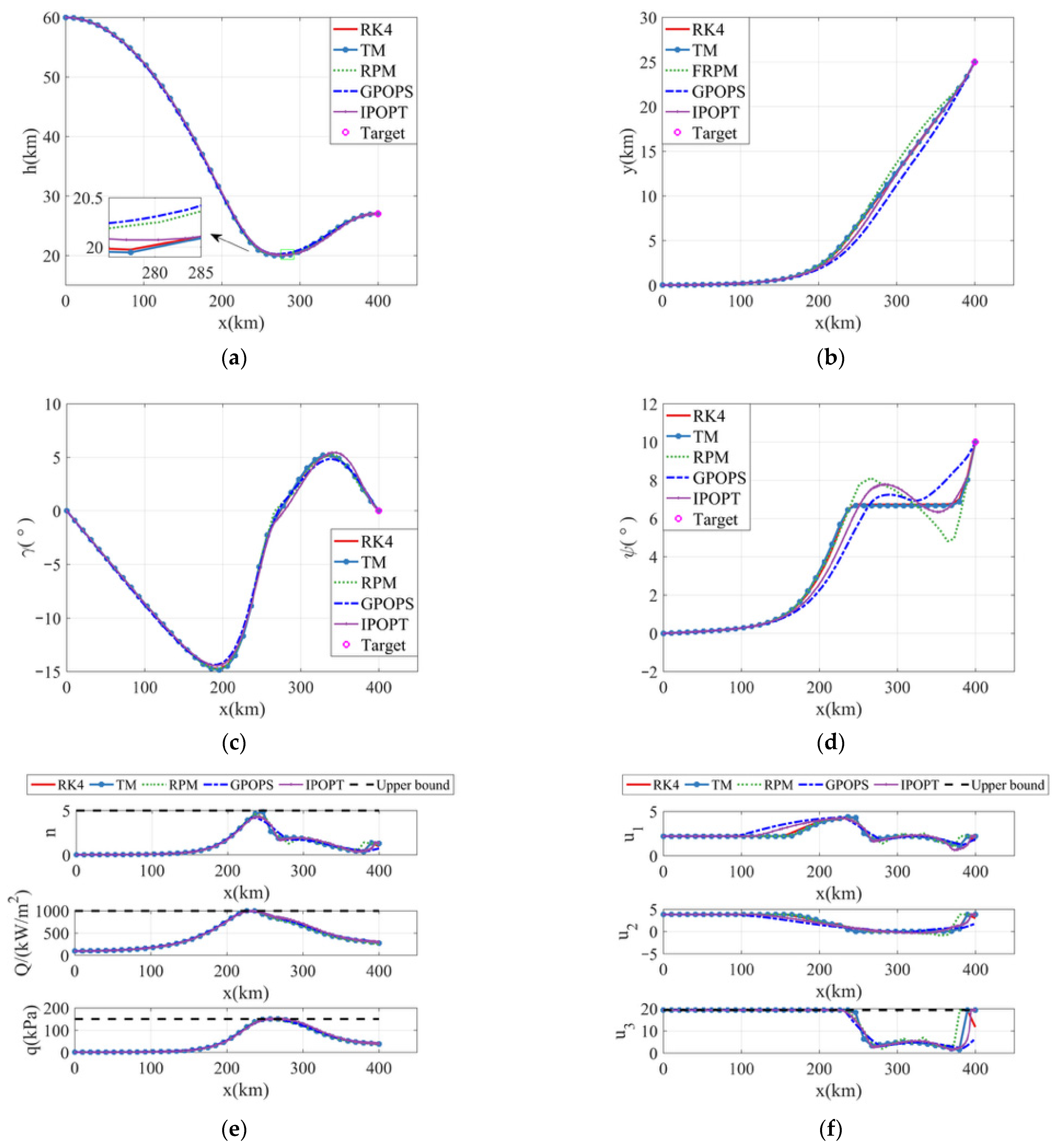
5.2. Method Performance Comparison

This section solved problem P2 using three SCP methods with different interpolation schemes: RK4, TM, and RPM. It also employed two fixed-terminal optimization methods: GPOPS and IPOPT. The performance of these approaches was then compared.

From Figure 4a,b, it can be observed that all methods generated similar trajectory shapes, successfully reaching the target position at the desired angle. Figure 4c,d shows the flight path angle and azimuth angle of the converged trajectories. The flight path angle distributions were nearly identical across methods. For heading angles, RPM, GPOPS, and IPOPT showed notable differences from the other methods. This divergence likely comes from their distinct discretization approaches and nonlinear optimization treatments. Figure 4e,f shows the process constraints and control quantities of the trajectories, which all conformed to the constraints, where the black dashed line is the maximum value of the constraints. On the whole, the simulation results of RK4 and TM were relatively similar, which was related to the equal spacing of discrete points. RPM, GPOPS, and IPOPT use non-equidistant discrete points, which are somewhat different from the previous two.

The performance of the different methods for solving problem P2 is shown in

Table 2. Comparison of results from the different methods.

Method	Run Time (ms)	Number of Iterations	Error on Position (m)	Error on Angle (°)
RK4	1511.6	4	8.5 × 10−6	6.5 × 10−13
TM	1468.2	4	2.1 × 10−4	1.9 × 10−11
RPM	1858.2	4	9.4 × 10−4	1.5 × 10−10
GPOPS	4814.6	\	0	0
IPOPT	5338.3	\	0	0

, and the running time was the average of 20 simulations. The RK4, TM, and PRM interpolation methods had similar terminal errors to solve problem P2, which can be ignored. Among the three methods, RPM took the longest time for a single iteration, and RK4 and TM had similar running times for a single iteration. The GPOPS and IPOPT methods had longer running times, and the optimized terminal error was 0 because the terminal relaxation constraint was not adopted. However, if the terminal constraint condition is changed, the GPOPS method may not be able to solve the trajectory. The effectiveness of the proposed method is verified in the next section. At 40 discrete points, with the GPOPS method as the standard, the TM method was 68.6% faster, the RK4 method was 69.5% faster, and PRM was 61.4% faster.

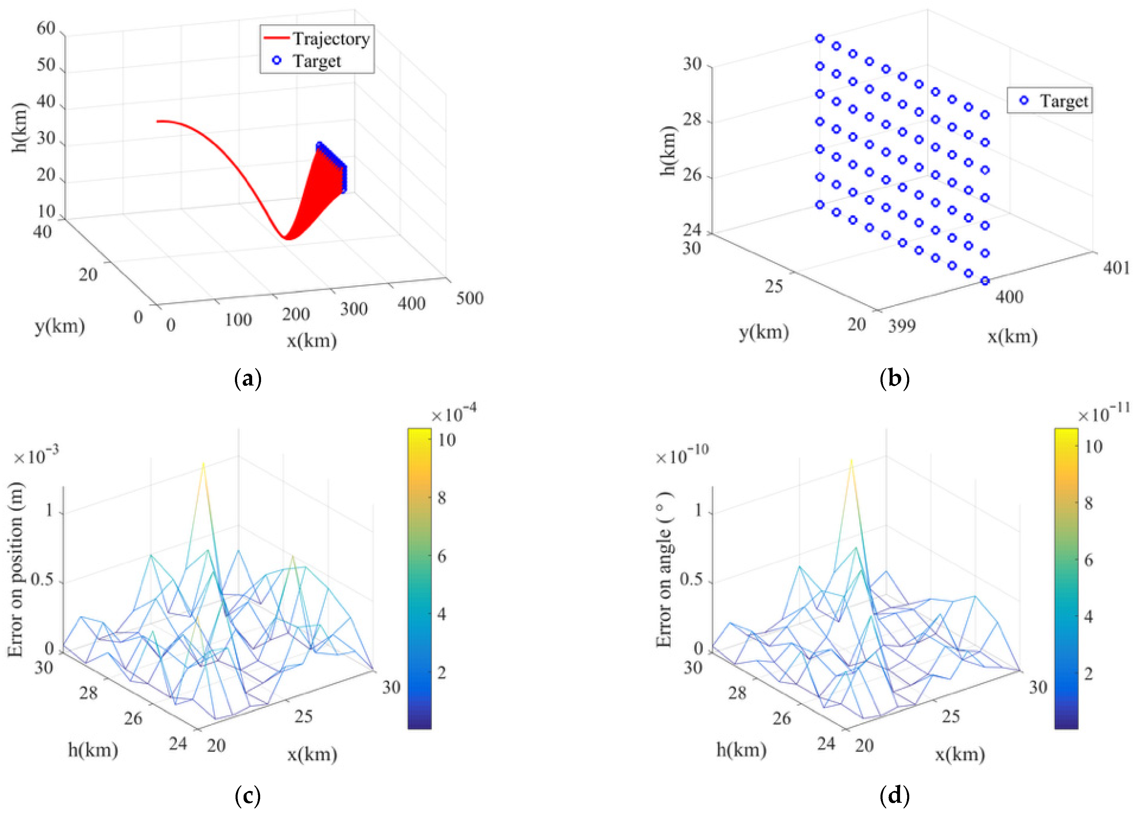
5.3. Validation of the Proposed Algorithm

The RK4 method was used to solve problem P2 under different terminal position constraints to verify the robustness of the proposed method. In this section, isometric selection of terminal position constraints was adopted, with the value of 20:0.5:30 in the z-axis direction and 24:0.5:30 in the h-axis direction, as shown in Figure 5b, and other simulation parameters remained unchanged.

Figure 5 shows that the proposed methods were capable of generating trajectories under the selected terminal position conditions. There was no infeasible solution, which shows that the proposed method is stable. It could generate the optimal midcourse guidance trajectory without modifying parameters according to specific terminal constraints. This demonstrates that our method can still effectively generate trajectories when only the terminal conditions are altered, while keeping all of the other parameters unchanged—a scenario that poses challenges for GPOPS. Figure 5c,d shows that the errors of different terminals were within a certain range, and that the optimization errors of position and angle may increase slightly on the boundary value. When the target point is far from the initial guess trajectory, the new initial guess trajectory can be selected as the reference trajectory. In engineering, the preset initial guess trajectory can be selected at medium spacing in space, or the optimized trajectory can be used as the initial guess trajectory to generate the trajectory to the ideal terminal state. The simulation results demonstrate that the proposed method can reliably achieve offline trajectory planning for midcourse guidance.

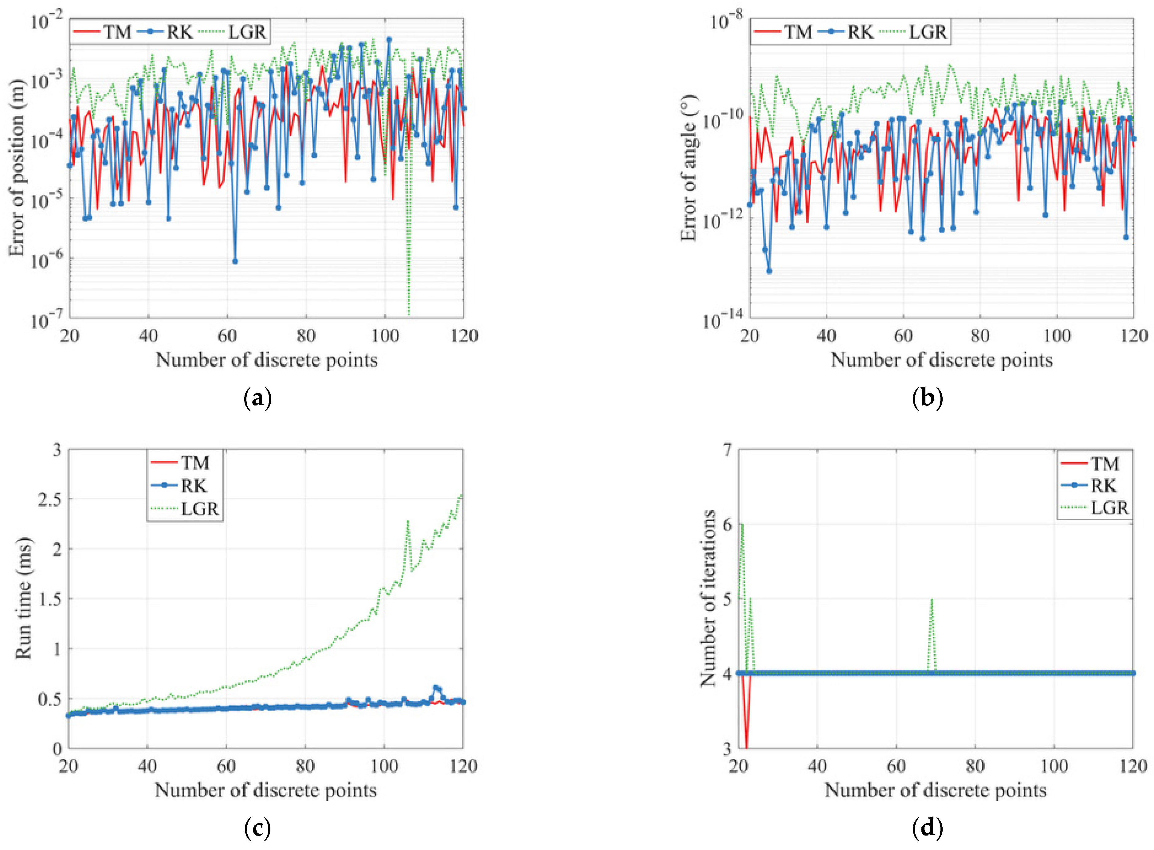
5.4. The Effect of Interpolation Method and the Number of Discrete Points

The simulation in this section mainly analyzed the effect of RK4, TM, RPM, and the number of discrete points on solving problem P2 in this paper. It can later be used as a reference for our own research and that of others. The terminal error is the difference between the trajectory terminal and the set target terminal.

Figure 6a,b shows the position error and angle error of the optimized trajectory. The terminal error of TM and RK4 was close. The optimization error of RPM was slightly worse than that of the TM and RK4 methods as a whole, but the optimization error was negligible for the vehicle volume. Figure 6c,d shows the single iteration running time and iteration number of different interpolation methods to solve problem P2. On the whole, the running time of a single iteration increased with the increase in the number of discrete points. The number of iterations showed no clear correlation with the number of discrete points. However, when fewer discrete points were used, the iteration count tended to exhibit more oscillations. The running time and iteration times of RK4 and TM were close, and the running time of RK4 was slightly larger than TM when the number of discrete points increased. The running time of RPM obviously increased with the number of discrete points, and the number of iterations was more overall. The more discrete points it had, its running time was significantly higher than RK4 and TM. Based on the positive correlation between the discretization node quantity, iteration count, and computation time, the trajectory generation duration can be regulated by optimizing these two key parameters.

The simulation results demonstrate that although no significant correlation exists between the iteration count and discretization node quantity, the computation time remains jointly influenced by these two parameters. This observed dependency facilitates the regulation of trajectory optimization duration through coordinated tuning of the node discretization density and prescribed iteration limit.

6. Conclusions

This paper addresses the challenges of dual-channel coupling and stringent terminal selection requirements in midcourse guidance trajectory design. A method for generating optimal midcourse guidance trajectories was proposed, employing range-domain affine control with terminal relaxation. The range-domain dynamic model eliminates dual-channel coupling in aerodynamically controlled vehicle without relying on angle of attack or altitude monotonicity. Terminal relaxation mitigates the strict trajectory terminal constraints imposed by limited aerodynamic maneuverability. Under reasonable assumptions, the maximum principle proves that the convexified SOCP problem is equivalent to the original nonconvex problem.

The simulation results demonstrated the effectiveness of the proposed method. Under identical initial guess trajectories and parameter constraints, the terminal state of the generated trajectory could be selected arbitrarily within a specified range. When considering process constraints in midcourse guidance with 40 discrete points, the time cost of a single iteration increased by 15.5%. Compared with the GPOPS method as a benchmark, with process constraints included, the TM method was 68.6% faster, the RK4 method was 69.5% faster, and the RPM method was 61.4% faster per iteration. Furthermore, RK4 and TM exhibited comparable computational efficiency. As the number of discrete points increased, RPM’s computational time grew significantly compared with both RK4 and TM. Future work will focus on optimizing discrete point selection based on midcourse guidance trajectory characteristics to further improve the computational efficiency.

References

1. Malyuta, D.; Yu, Y.; Elango, P.; Açıkmeşe, B. Advances in trajectory optimization for space vehicle control. Annu. Rev. Control 2021, 52, 282–315. [Google Scholar] [CrossRef]
2. Bu, X.W.; Lv, M.L.; Lei, H.M.; Cao, J. Fuzzy neural pseudo control with prescribed performance for waverider vehicles: A fragility-avoidance approach. IEEE Trans. Cybern. 2023, 53, 4986–4999. [Google Scholar] [CrossRef]
3. Kim, B.; Lee, C.-H. Optimal midcourse guidance for dual-pulse rocket using pseudospectral sequential convex programming. J. Guid. Control Dyn. 2023, 46, 1425–1436. [Google Scholar] [CrossRef]
4. Zhou, C.; He, L.; Yan, X.; Meng, F.; Li, C. Active-set pseudospectral model predictive static programming for midcourse guidance. Aerosp. Sci. Technol. 2023, 134, 108137. [Google Scholar] [CrossRef]
5. Wan, S.X.; Chang, X.F.; Li, Q.C.; Yan, J. Suboptimal midcourse guidance with terminal-angle constraint for hypersonic target interception. Int. J. Aerosp. Eng. 2019, 2019, 6161032. [Google Scholar] [CrossRef]
6. Calise, A.J. Adaptive finite time intercept guidance. J. Guid. Control Dyn. 2023, 46, 1975–1980. [Google Scholar] [CrossRef]
7. Shin, H.S.; Li, K.B. An improvement in three-dimensional pure proportional navigation guidance. IEEE Trans. Aerosp. Electron. Syst. 2021, 57, 3004–3014. [Google Scholar] [CrossRef]
8. Chen, J.; Zhao, Q.; Liang, Z.; Li, P.; Ren, Z.; Zheng, Y. Fractional calculus guidance algorithm in a hypersonic pursuit-evasion game. Def. Sci. J. 2017, 67, 688–697. [Google Scholar] [CrossRef]
9. Liu, S.; Yan, B.; Liu, R.; Dai, P.; Yan, J.; Xin, G. Cooperative guidance law for intercepting a hypersonic target with impact angle constraint. Aeronaut. J. 2022, 126, 1026–1044. [Google Scholar] [CrossRef]
10. Liu, S.; Yan, B.; Zhang, T.; Dai, P.; Liu, R.; Yan, J. Three-dimensional cooperative guidance law for intercepting hypersonic targets. Aerosp. Sci. Technol. 2022, 129, 107815. [Google Scholar] [CrossRef]
11. Yao, D.; Xia, Q. Finite-Time Convergence Guidance Law for Hypersonic Morphing Vehicle. Aerospace 2024, 11, 680. [Google Scholar] [CrossRef]
12. Xi, A.; Cai, Y. A nonlinear finite-time robust differential game guidance law. Sensors 2022, 22, 6650. [Google Scholar] [CrossRef] [PubMed]
13. Yang, B.; Jing, W.; Gao, C. Online midcourse guidance method for boost phase interception via adaptive convex programming. Aerosp. Sci. Technol. 2021, 118, 107037. [Google Scholar] [CrossRef]
14. Chai, R.; Tsourdos, A.; Savvaris, A.; Chai, S.; Xia, Y.; Chen, C.P. Review of advanced guidance and control algorithms for space/aerospace vehicles. Prog. Aerosp. Sci. 2021, 122, 100696. [Google Scholar] [CrossRef]
15. Liu, G.; Feng, W.; Yang, K.; Zhao, J. Hybrid QPSO and SQP algorithm with homotopy method for optimal control of rapid cooperative rendezvous. J. Aerosp. Eng. 2019, 32, 04019030. [Google Scholar] [CrossRef]
16. Ann, S.; Lee, S.; Kim, Y.; Ahn, J. Midcourse guidance for Exoatmospheric Interception Using Response Surface based trajectory shaping. IEEE Trans. Aerosp. Electron. Syst. 2020, 56, 3655–3673. [Google Scholar] [CrossRef]
17. Kasmi, H.; Laporte, S.; Mongeau, M.; Vidosavljevic, A.; Delahaye, D. Holistic approach for vehicle trajectory optimization using optimal control. J. Veh. 2023, 60, 1302–1313. [Google Scholar]
18. Chai, R.; Savvaris, A.; Tsourdos, A.; Chai, S.; Xia, Y. A review of optimization techniques in spacecraft flight trajectory design. Prog. Aerosp. Sci. 2019, 109, 100543. [Google Scholar] [CrossRef]
19. Dennis, M.E.; Hager, W.W.; Rao, A.V. Computational method for optimal guidance and control using adaptive Gaussian quadrature collocation. J. Guid. Control Dyn. 2019, 42, 2026–2041. [Google Scholar] [CrossRef]
20. Luo, C.X.; Zhou, C.J.; Bu, X.W. Multi-Missile Phased Cooperative Interception Strategy for High-Speed and Highly Maneuverable Targets. IEEE Trans. Aerosp. Electron. Syst. 2025, 61, 1971–1996. [Google Scholar] [CrossRef]
21. Zhou, C.; Yan, X.; Ban, H.; Tang, S. Generalized Newton Iteration based MPSP Method for Terminal Constrainted Guidance. IEEE Trans. Aerosp. Electron. Syst. 2023, 59, 9438–9450. [Google Scholar] [CrossRef]
22. Mondal, S.; Padhi, R. Angle-constrained terminal guidance using quasi-spectral model predictive static programming. J. Guid. Control Dyn. 2018, 41, 783–791. [Google Scholar]
23. Chai, R.; Tsourdos, A.; Savvaris, A.; Chai, S.; Xia, Y. Solving constrained trajectory planning problems using biased particle swarm optimization. IEEE Trans. Aerosp. Electron. Syst. 2021, 57, 1685–1701. [Google Scholar] [CrossRef]
24. Li, W.L.; Li, J.; Li, N.B.; Shao, L.; Li, M.J. Online trajectory planning method for midcourse guidance phase based on deep reinforcement learning. Aerospace 2023, 10, 441. [Google Scholar] [CrossRef]
25. Li, H.; Wang, J.; Tao, H.; Lin, D. Near-Optimal Impact-Vector-Control Guidance. J. Guid. Control Dyn. 2024, 47, 1965–1972. [Google Scholar] [CrossRef]
26. Kada, B.; Ansari, U.; Bajodah, A.H. Highly maneuvering target interception via robust generalized dynamic inversion homing guidance and control. Aerosp. Sci. Technol. 2020, 99, 105749. [Google Scholar] [CrossRef]
27. Annam, C.; Ratnoo, A.; Ghose, D. Singular-perturbation-based guidance of pulse motor interceptors with look angle constraints. J. Guid. Control Dyn. 2021, 44, 1356–1370. [Google Scholar] [CrossRef]
28. Wang, Z. A survey on convex optimization for guidance and control of vehicular systems. Annu. Rev. Control 2024, 57, 100957. [Google Scholar] [CrossRef]
29. Kayama, Y.; Howell, K.C.; Bando, M.; Hokamoto, S. Low-thrust trajectory design with successive convex optimization for libration point orbits. J. Guid. Control Dyn. 2022, 45, 623–637. [Google Scholar] [CrossRef]
30. Zhou, X.; Zhang, H.-B.; Xie, L.; Tang, G.-J.; Bao, W.-M. An improved solution method via the pole-transformation process for the maximum-crossrange problem. Proc. Inst. Mech. Eng. Part G J. Aerosp. Eng. 2020, 234, 1491–1506. [Google Scholar] [CrossRef]
31. Niu, G.; Wu, L.; Gao, Y.; Pun, M.-O. Unmanned aerial vehicle (UAV)-assisted path planning for unmanned ground vehicles (UGVs) via disciplined convex-concave programming. IEEE Trans. Veh. Technol. 2022, 71, 6996–7007. [Google Scholar] [CrossRef]
32. Mousavi, S.M.A.; Moshiri, B.; Heshmati, Z. On the distributed path planning of multiple autonomous vehicles under uncertainty based on model-predictive control and convex optimization. IEEE Syst. J. 2020, 15, 3759–3768. [Google Scholar] [CrossRef]
33. Liu, X.; Shen, Z.; Lu, P. Exact convex relaxation for optimal flight of aerodynamically controlled missiles. IEEE Trans. Aerosp. Electron. Syst. 2016, 52, 1881–1892. [Google Scholar] [CrossRef]
34. Yang, R.; Liu, X.; Song, Z. Rocket landing guidance based on linearization-free convexification. J. Guid. Control Dyn. 2024, 47, 217–232. [Google Scholar] [CrossRef]
35. Ma, S.; Yang, Y.; Tong, Z.; Yang, H.; Wu, C.; Chen, W. Improved sequential convex programming based on pseudospectral discretization for entry trajectory optimization. Aerosp. Sci. Technol. 2024, 152, 109349. [Google Scholar] [CrossRef]
36. Wang, Z.; Grant, M.J. Autonomous entry guidance for hypersonic vehicles by convex optimization. J. Spacecr. Rocket. 2018, 55, 993–1006. [Google Scholar] [CrossRef]
37. Liu, X.; Lu, P.; Pan, B. Survey of convex optimization for aerospace applications. Astrodynamics 2017, 1, 23–40. [Google Scholar] [CrossRef]
38. Wang, Q.; Li, S.; Zhang, Y.; Cheng, M. Spacecraft Close Proximity to Noncooperative Target Based on Pseudospectral Convex Method. J. Aerosp. Eng. 2024, 37, 04024034. [Google Scholar] [CrossRef]
39. Zhou, X.; He, R.-Z.; Zhang, H.-B.; Tang, G.-J.; Bao, W.-M. Sequential convex programming method using adaptive mesh refinement for entry trajectory planning problem. Aerosp. Sci. Technol. 2021, 109, 106374. [Google Scholar] [CrossRef]
40. Liu, X. Convergence-guaranteed trajectory planning for a class of nonlinear systems with nonconvex state constraints. IEEE Trans. Aerosp. Electron. Syst. 2021, 58, 2243–2256. [Google Scholar] [CrossRef]
41. Tang, G.; Jiang, F.; Li, J. Fuel-optimal low-thrust trajectory optimization using indirect method and successive convex programming. IEEE Trans. Aerosp. Electron. Syst. 2018, 54, 2053–2066. [Google Scholar] [CrossRef]
42. Wang, Z.; Lu, Y. Improved sequential convex programming algorithms for entry trajectory optimization. J. Spacecr. Rocket. 2020, 57, 1373–1386. [Google Scholar] [CrossRef]
43. Liu, X.; Shen, Z.; Lu, P. Entry trajectory optimization by second-order cone programming. J. Guid. Control Dyn. 2016, 39, 227–241. [Google Scholar] [CrossRef]
44. NASA. U.S. Standard Atmosphere, 1976; NASA Technical Memorandum X-74335; NASA: Washington, DC, USA, 1976.
45. Li, H.F. Guidance and Control Technology for Hypersonic Vehicles; China Astronautic Publishing House: Beijing, China, 2012. [Google Scholar]
46. Domahidi, A.; Chu, E.; Boyd, S. ECOS: An SOCP solver for embedded systems. In Proceedings of the 2013 European Control Conference (ECC), Zurich, Switzerland, 17–19 July 2013; pp. 3071–3076. [Google Scholar]
47. Wächter, A.; Biegler, L.T. On the Implementation of a Primal-Dual Interior Point Filter Line Search Algorithm for Large-Scale Nonlinear Programming. Math. Program 2006, 106, 25–57. [Google Scholar] [CrossRef]
48. Hartl, R.F.; Sethi, S.P.; Vickson, R.G. A survey of the maximum principles for optimal control problems with state constraints. SIAM Rev. 1995, 37, 181–218. [Google Scholar] [CrossRef]
Figure 1. Trajectory in the lateral range domain.
Aerospace 12 00618 g001
Figure 2. Schematic diagram of the original control set and the relaxed control set. (a) Horizontal section of the original control set; (b) relaxed control set horizontal section; (c) original control set; (d) relaxed control set.
Aerospace 12 00618 g002
Figure 3. Convergence graph of the algorithm with and without process constraints. (a) Longitudinal trajectories; (b) lateral trajectories; (c) longitudinal trajectories; (d) lateral trajectories; (e) error on position; (f) error on angle.
Aerospace 12 00618 g003aAerospace 12 00618 g003b
Figure 4. Convergence trajectories of different methods. (a) Longitudinal trajectories; (b) lateral trajectories; (c) flight path angle; (d) heading angle; (e) constraints on process; (f) control instruction.
Aerospace 12 00618 g004
Figure 5. Simulation under different terminal conditions. (a) Three dimensional trajectories; (b) position terminals; (c) position error; (d) angle error.
Aerospace 12 00618 g005
Figure 6. Simulation of different interpolation methods and number of discrete points. (a) Error on position; (b) error on angle; (c) average iteration run time; (d) number of iterations.
Aerospace 12 00618 g006