1. Introduction
The optimal control theory has been widely studied since its first appearance. It has been applied in mechanical [
1], aerospace [
2], chemical [
3], and other engineering fields through continuous development. In the aerospace field, numerous complicated and critical problems can be described in the form of optimal control problems (OCPs), which include attitude control [
4] and trajectory optimization [
5,
6]. As the complexity of problems increases, previous optimal control methods face challenges in providing rapid and accurate solutions, particularly when computational resources are limited. Therefore, it is necessary to study more efficient and innovative solving methods.
In recent years, the pseudospectral method has become an important method to solve nonlinear OCPs, owing to its high computational accuracy and fast convergence [
7,
8,
9,
10,
11]. The pseudospectral method, as a direct method, approximates global state and control variables with orthogonal polynomials, thereby transforming the differential equations into a set of linear algebraic equations. In addition to the various constraints and performance indices after transformation, the original nonlinear optimal control problem can be transformed into a nonlinear programming (NLP) problem, which can be solved using mature nonlinear optimization solvers such as SNOPT and IPOPT [
12,
13,
14,
15,
16,
17,
18]. Moreover, the pseudospectral method has some great characteristics, such as accurate estimation of the costates, the equivalence between the first-order necessary condition of the transformed NLP problem and the Karush–Kuhn–Tucker (KKT) condition of the original OCP [
19,
20], and a well-established convergence proof [
21]. Pseudospectral methods are categorized into the Legendre Pseudospectral Method (LPM), Gauss pseudospectral method (GPM), Radau pseudospectral method (RPM), and Chebyshev Pseudospectral Method (CPM) according to different orthogonal polynomial collocations [
22,
23]. However, NLP solvers consume significant memory and computational resources, and they cannot guarantee the feasibility of each step in the computation process. Additionally, if the initial guess provided is not sufficiently accurate, the computational time cannot be guaranteed within a specified limit. Therefore, the pseudospectral method is suitable for offline optimization [
24,
25].
In order to solve the nonlinear OCP online, Padhi et al. proposed a method for solving finite-time nonlinear OCPs with terminal constraints, known as model predictive static programming (MPSP), combining the idea of nonlinear model predictive control (MPC) and approximate dynamic programming [
26]. This method predicts terminal errors through numerical integration and discretization dynamics using the Euler integration. It has been successfully applied to many problems in the aerospace field [
27,
28]. However, this approach requires a large number of nodes to ensure the computational accuracy, which leads to low computational efficiency. Yang et al. also proposed a linear Gauss pseudospectral model predictive control method (LGPMPC) on the framework of MPC, which can solve the nonlinear OCP with fixed time [
29]. In comparison with MPSP, this method employs orthogonal collocation points, requiring fewer nodes for the same accuracy, and only needs to solve linear algebraic equations through linearization, which has higher computational efficiency and can be applied online. This method has also been developed and applied in various scenarios such as reentry guidance [
30] and long-term air-to-air missile guidance [
31,
32]. Also, scholars use a pseudospectral discretization strategy to reduce the requirement of the number of nodes for MPSP [
33]. However, both of the above methods require a performance index in the form of linear quadratic, and their costate variables are not the same as those of the original OCP. Therefore, they cannot solve OCPs with arbitrary performance indices or provide the costate variables of the original problem.
Convex optimization methods have also been widely applied in the field of guidance control due to their global optimality and convergence properties. Tang et al. proposed an optimization scheme for solving the fuel-optimal control problem by combining the indirect method with the successive convex programming [
34]. Wang et al. proposed improved sequential convex programming algorithms based on line-search and trust-region methods to address constrained entry trajectory optimization problems [
35]. Some researchers have also studied the combination of pseudospectral methods and convex optimization to improve accuracy. Sagliano investigated the Mars-powered descent problem using the pseudospectral convex optimization method [
36]. Li et al. combined Chebyshev pseudospectral discretization with successive convex optimization to propose an online guidance method, which was applied to orbit transfer problems [
37]. However, the use of convex optimization methods requires problem convexification, and the inner iterations of sequential convex optimization consume significant computational resources. The online computational efficiency of this method needs to be further improved.
The neighboring extremal optimal method was proposed in the 1960s [
38,
39], which can obtain the feedback correction when the parameters of the OCP are disturbed. Given the precalculated nominal optimal solution, this method can provide a first-order approximation of the optimal solution for perturbations in initial states and terminal constraints by minimizing the quadratic variation of the performance index. Typically, this method employs a Riccati transformation and backward sweep to solve the linearized quadratic problem derived from the original problem, yielding linear feedback gains [
40,
41]. However, due to the necessity of solving the Riccati matrix differential equations formed during the backward sweep process, the computational efficiency is too low to be applied online. In recent years, many scholars have focused on improving the computational efficiency of the neighboring extremal method [
42,
43,
44,
45,
46].
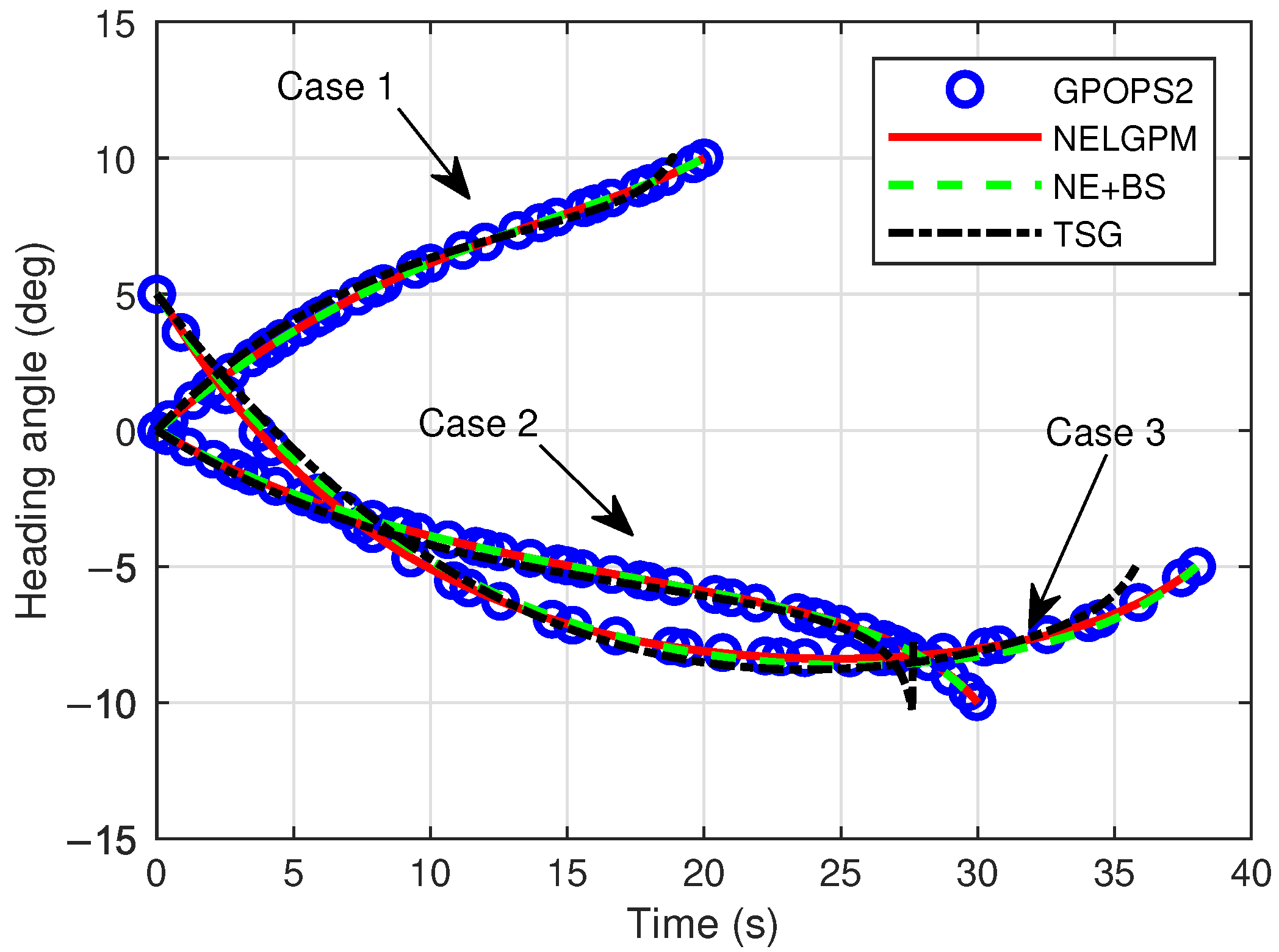
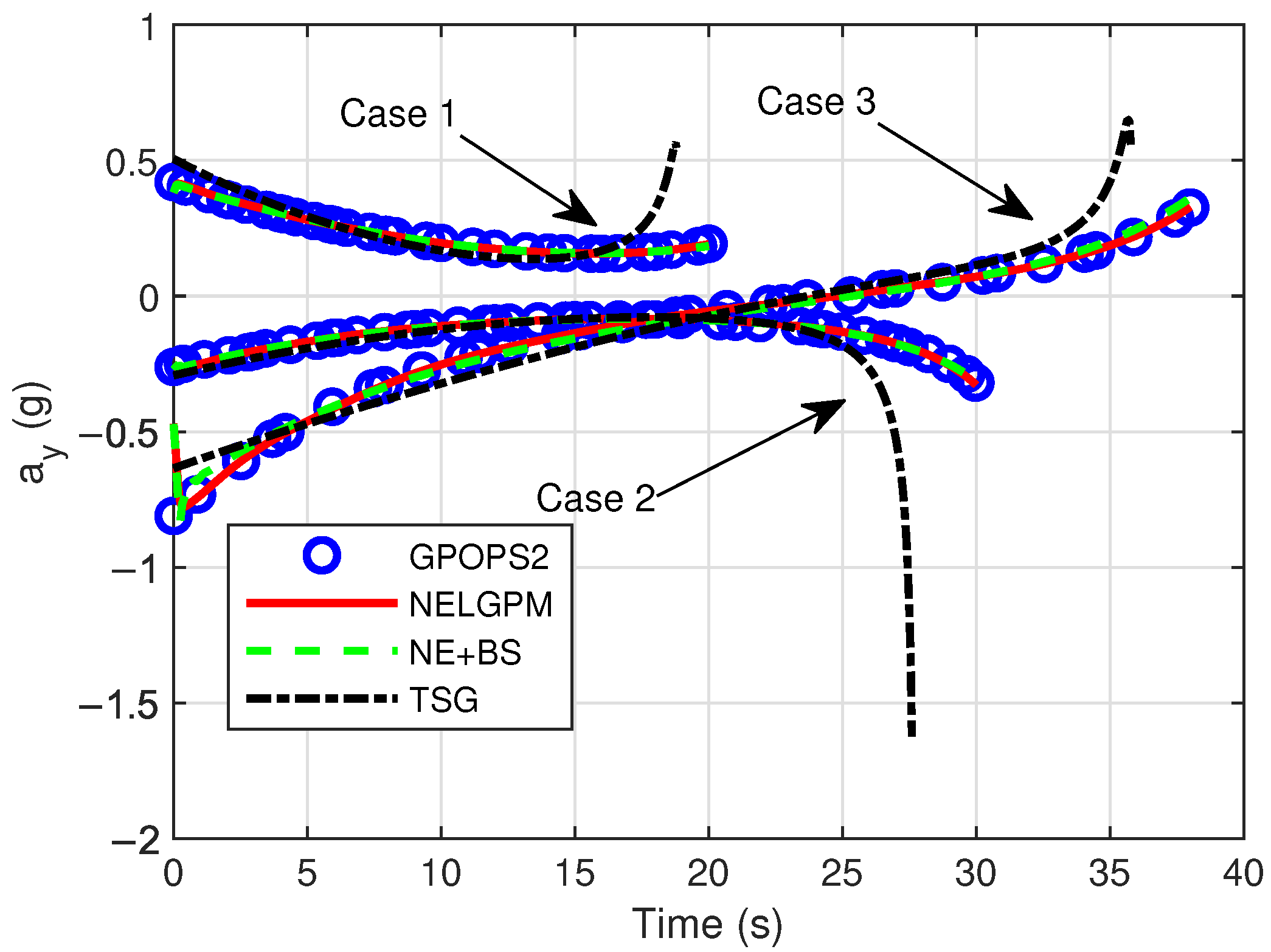
Inspired by LGPMPC and the neighboring extremal method, this paper proposes an efficient algorithm to solve nonlinear OCPs online with arbitrary performance indices. It is referred to as the neighboring extremal linear Gauss pseudospectral method (NELGPM). The main contributions of this paper are as follows: Firstly, the deviations in initial states and terminal constraints are fully considered. A quadratic performance index involving the second-order variation of the original nonlinear performance index is formulated through the variational principle and linearization around the nominal optimal solution. Secondly, the perturbation differential equations involving the deviations between the neighboring extremal path and the original optimal solution are derived via the first-order necessary conditions. Then, an OCP with a quadratic performance index and boundary constraints is formulated. Thirdly, the Gauss pseudospectral collocation is utilized to discretize the quadratic OCP, thereby transforming it into a set of linear algebraic equations including deviations in state and costate variables. Furthermore, on the polynomial space, an analytical solution of the control correction can be successfully derived to come close to the nonlinear optimal solution for the original OCP. Because of discretization at orthogonal points, this process is characterized by high computation speed and low computational complexity, which makes it suitable for online applications. The main difference from previous work is that the proposed method can solve OCP with an arbitrary performance index and provide costate information of optimal control, which greatly expands the scope of applications. Finally, the terminal guidance problem is applied to verify the performance of the proposed method. Some simulations and comparisons have been performed. The results show that it has not only high computational efficiency and accuracy, but also optimality for an arbitrary performance index. Additionally, Monte Carlo simulations have been carried out. The results demonstrate that the proposed method, even in highly dispersed environments, has good adaptability and robustness. Furthermore, NELGPM has great potential for real-time online applications.
The chapters of this paper are organized as follows:
Section 2 and
Section 3 introduce the problem formulation and the theory of neighboring extremal optimal control. Next, the solving process of pseudospectral discretization and the derivation of the control correction formula are described in detail.
Section 4 is the simulation and discussion, and
Section 5 presents the conclusion.
2. Problem Formulation
For an OCP with fixed terminal time and terminal constraints, the state differential equations are given by
where
is the state vector,
is the control vector, and
is the time variable.
And terminal constraints are
where
is the number of fixed state variables at the terminal,
are the fixed terminal values, and
is the terminal time and is also fixed.
The performance index is
where
is the initial time,
is the initial state, and
and
L are known scalar functions. Equations (
1)–(
3) describe a general fixed-time OCP, which is to identify a set of control variables
that minimize the performance index
J.
For the OCP as above, it is known from the optimal control theory that the optimal solution is determined by the following first-order necessary conditions. The Hamiltonian function
H can be expressed as
where
is the costate vector. State equations, costate equations, and control equations are
The transversality conditions are
where
is the Lagrange multiplier associated with the terminal constraints. According to (
2) and (
6), if the variable
is not terminally constrained, then
where
. If the variable
is terminally constrained, then
The solution to the original OCP can be obtained by solving the two-point boundary value problem (TPBVP) consisting of this set of equations and boundary conditions. However, if the problem is nonlinear, it is very difficult to solve in an analytical manner. Moreover, numerical iterative methods are typically used to solve such problems.
3. Neighboring Extremal Linear Gauss Pseudospectral Method
3.1. Neighboring Extremal Optimal Control
It is known that the optimal solution for a general OCP varies with changes in initial states and terminal conditions. On the assumption of small disturbances, the neighboring extremal method can provide the solution approaching the optimal solution for the problem when the initial states and terminal conditions are changed.
Considering differential equation constraints (
1) and terminal constraints (
2), the augmented performance index can be expressed as
Considering the initial state deviations
and terminal deviations
, the increment of
with respect to changes in control
can be expressed as
where
,
,
,
, etc. Because of the approximation around the nominal optimal solution, the coefficients satisfy the previous first-order necessary conditions. So (
10) can be simplified to
where all the coefficients are calculated according to the optimal solution.
From (
11), it can be seen that
and
are the first-order functions of the performance index
J with respect to the initial state deviations
and terminal deviations
.
The second-order terms on the right-hand side of (
11) can be interpreted as the second-order variation of the original problem, which can be seen as solving a new OCP with a quadratic performance index (
12), that is, by selecting
to obtain the neighboring extremal path whose initial and terminal conditions are slightly different from the optimal path. The neighboring extremal path satisfies the following linear perturbation equation:
The coefficients of this equation are also calculated according to the original optimal solution. The boundary conditions for this new OCP are
Considering the differential equation constraints (
13) and terminal constraints (
15), the new augmented performance index can be expressed as
where
and
are the deviations of the Lagrange multipliers in the original problem. Now fixing initial state deviations
and terminal deviations
, the increment of
with respect to
and
is expressed as follows:
Neglecting high-order terms in (
17), we can obtain the necessary condition for the new OCP.
The linear TPBVP formed by Equations (
18)–(
20) and (
13)–(
15) determines the neighboring extremal path with given initial state deviations and terminal deviations. From the above derivations, it can be inferred that the solutions to the TPBVP can minimize (or maximize) the second-order variation of the original OCP. As indicated by (
11), the first-order deviation terms are independent of control variables. However, changes in control derived from the second-order deviation terms yield the optimal adjustments. Assuming
is nonsingular, the control updates can be represented as follows:
According to Legendre’s condition, the second-order variation takes the minimum value if
. When
,
is nonsingular. Substituting (
21) into (
13) and (
18) yields a set of differential equations only related to
and
, expressed as follows:
where
The boundary conditions are as shown in (
24).
In the past, the conventional approach for solving the aforementioned linear TPBVP was the backward sweep method. Actually, the backward sweep method requires multiple numerical integrations, including solving a set of Riccati matrix differential equations. Additionally, to ensure accuracy and numerical stability, it also requires a sufficiently large number of integration nodes. These restrict the application of the neighboring extremal method. In response, this paper proposes a new method for efficiently solving this problem after linearization in polynomial space.
3.2. Pseudospectral Collocation Scheme of NELGPM
For the perturbed differential Equation (
22), the linear Gauss pseudospectral discretization strategy is used to discretize it and transform it into a set of linear equations, so that the changes in state variables and costate variables at each discrete node can be solved efficiently. Then the correction of control variables can be calculated from (
21) to correct the disturbance.
Gaussian quadrature is a widely used integration method, known for its high computational accuracy with few nodes. In this method, the supporting nodes are the zeros of orthogonal polynomials. In this paper, we utilize a Legendre-type Gaussian quadrature, whose zeros range within
. Thus, the initial step involves transforming the original problem’s time domain from
to
. The transformation formula is as follows:
The performance index and Hamiltonian function are also transformed into the new time domain, yielding the following outcomes:
Equation (
22) is also transformed into the following form:
As stated above, the discrete nodes are chosen as the zeros of orthogonal polynomials. Let the order of the orthogonal polynomials be
N, and
(
) are the zeros of the
Nth-order Legendre orthogonal polynomials, also known as LG (Legendre–Gauss) nodes. From these zeros, two sets of
Nth-order Lagrange polynomials
and
can be obtained, which exhibit a certain conjugate relationship.
Consequently, the variations in state variables, control variables, and costate variables can be expressed through Lagrange interpolation polynomials as shown in (
29), where
,
, and
represent the respective variable values at the discrete nodes and
,
, and
represent the result after using the
Nth-order Lagrange interpolation polynomial.
From the Lagrange interpolation polynomial, we can obtain
It is obvious that the Lagrange polynomials satisfy the requirements at the interpolation nodes.
Upon differentiating the Lagrange interpolation polynomials (
29) at the discrete nodes, the expressions for the derivatives of the change in state variables and costate variables at the LG nodes are obtained as follows:
where
,
. Simultaneously, this process also yields a differential approximation matrix
of size
.
D and
possess a certain adjoint relationship, which can be determined through the following formula:
where
and
are the quadrature coefficients of the Gaussian quadrature formula, and
is the element in the first column of
D.
Substituting (
32) into (
28), and incorporating the relationship between the initial and terminal deviations yields the following set of linear algebraic equations:
where
.
,
and
represent the values of the
A,
B, and
C matrices at the
k-th node. Note that the boundary nodes are not all included in the dynamic constraints. Therefore, two additional constraints are added to (
34), so that the terminal state deviations and costate deviations satisfy the dynamic equation constraints through Gaussian quadrature.
This set of equations shows that there is a certain linear relationship between the state and costate deviations of the neighboring extremal path and the original optimal path, so we can describe the state and costate deviations at all nodes in analytic form and compute the control corrections at all nodes via (
21).
3.3. Derivations of Analytical Correction Formula for Control
In this section, we derive the analytical control correction formula to eliminate errors and come close to the optimal solution.
Then we can use
to represent the state and costate deviations at all nodes. In order to obtain the analytical control correction formula,
must first be derived from (
34).
The first set of equations from (
34) can be written in the following form:
where
,
. Similarly, the third set of equations from (
34) can be expressed as follows:
where
,
. Combining (
36) and (
37) yields
where
.
k takes 1 to
N, and the
N equations in (
38) can be simultaneously written as
where
where
s represents the number of state variables.
In this way, we convert part of the equations in (
34) to the form with
as the unknown quantity, and the remaining one is related to the initial state deviations and the terminal costate deviations.
Combining the second and fourth equations from (
34), we obtain
Equation (
43) shows the relationship between the deviations in the initial and terminal times and that in the intermediate discrete nodes.
From (
39), if
is invertible, we obtain
Substituting (
45) into (
43) and eliminating the unknown quantity
yields
Define
, and
,
,
, and
are
s-order submatrices. Then (
46) can be simplified to
It is obvious that (
47) involves only the deviations in the initial and terminal time. The
is completely determined by the nominal trajectory.
If
is invertible, the following expressions can be obtained according to (
47):
From the boundary conditions (
24), the deviations of terminal state variables
can be calculated via terminal deviations
. Then, by using (
48), the initial and terminal deviations of the costate variables
and
can be obtained. Finally, substituting
and
into (
45), the deviations of state and costate variables
at all discrete nodes can be calculated.
From (
35), the values of
at each node can be obtained. Then substituting
into (
21), the control corrections at all discrete nodes can be obtained as shown in (
49).
where
.
Subsequently, through Lagrange interpolation (
29), the control corrections
at any given time can be obtained, thereby obtaining the complete control sequence
for the neighboring extremal path that minimizes the performance index of the original problem under the given initial and terminal deviations.
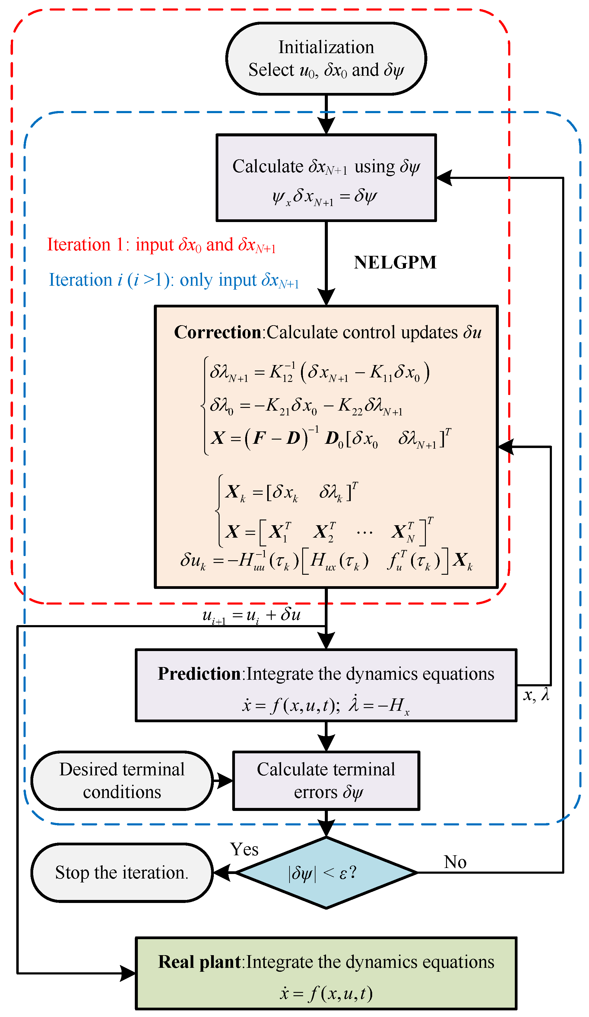
3.4. Implementation Steps
This paper presents the NELGPM for solving the nonlinear optimal control problem with an arbitrary performance index. It iteratively minimizes the second-order variation of the performance index with the constraints on perturbation equations. An analytical solution for this subproblem can be successfully derived in the polynomial space via Gauss pseudospectral collocation. Therefore, it has excellent computational efficiency and accuracy with few discrete points. The implementation steps of the proposed method are demonstrated in
Figure 1.
The specific algorithm flow is as follows.
Step 1: Determine the initial optimal trajectory and control, and set the initial state deviations and terminal errors .
Step 2: Calculate the terminal state deviations
according to terminal errors
. Then, based on the standard trajectory, calculate the neighboring extremal control updates from the initial deviations
and the terminal deviations
using (
45), (
48), and (
49).
Step 3: Integrate the dynamics differential equations with the updated controls, and record the new trajectory and terminal errors .
Step 4: Calculate the terminal state deviations
using the new terminal errors
. Substitute the terminal state deviations and updated trajectory into (
45), (
48), and (
49) to calculate control updates. At this stage, the initial deviations are set to zero.
Step 5: Take the updated control as the current control and return to step 3. Evaluate whether the terminal error accuracy meets the requirement. If it does, the algorithm terminates; if not, the algorithm continues.
Through the above steps, it can provide the iterative solution coming closer to the optimal solution for the original optimal control problem with the constraints on initial and terminal deviations. It should be noted that the algorithm requires an approximately optimal reference trajectory using the given performance index as the initial trajectory, which can be obtained through offline optimization algorithms.
In addition, according to (
23) and (
45), the computation of control correction requires some matrices to be nonsingular. Since we need to obtain the optimal solution in advance, the problems chosen for study are all normal optimal control problems. In this case, the matrices generated during the process will not be singular.


