Abstract
Modeling of wall-bounded turbulent flows, in particular the hybridization of the Reynolds-averaged Navier-Stokes (RANS) and large eddy simulation (LES) methods, has faced serious questions for decades. Specifically, there is continuous research of how usually applied methods such as detached eddy simulation (DES) and wall-modeled LES (WMLES) can be made more successful in regard to complex, high-Reynolds-number () flow simulations. The simple question is how it is possible to enable reliable and cost-efficient predictions of high- wall-bounded turbulent flows in particular under conditions where data for validation are unavailable. This paper presents a strict analysis of strategies for the design of seamlessly resolving turbulent flow simulations for a wide class of turbulence models. The essential conclusions obtained are the following ones: First, by construction, usually applied methods like DES are incapable of systematically spanning the range from modeled to resolved flow simulations, which implies significant disadvantages. Second, a strict solution for this problem is given by novel continuous eddy simulation (CES) methods, which perform very well. Third, the design of a computational simplification of CES that still outperforms DES appears to be very promising.
1. Introduction
The introduction of two-equation Reynolds-averaged Navier-Stokes (RANS) turbulence models by Kolmogorov [1] has marked a milestone in turbulence research. Such models involve two basic ingredients: an equation for the kinetic energy of turbulence k (which reflects the intensity of turbulent velocity fluctuations) and an equation for the scale of turbulence (an equation for the dissipation rate of turbulent kinetic energy, or the turbulence dissipation time scale , or the turbulence frequency , or the turbulence length scale ). The structure of the transport equation for k is well established, but there is still significant uncertainty about the most appropriate scale variable that should be considered in conjunction with k and the appropriate structure of the scale variable equation [2,3,4,5]. The most common structure of scale equations currently applied follows simple return-to-equilibrium concepts [6,7] similar to the Bhatnagar–Gross–Krook (BGK) approximation [8] of the Boltzmann equation.
Interestingly, Kolmogorov [1] did not include a production term in his -equation. Rotta [9,10] made an attempt to provide a solution to these questions from a fundamental view point; he developed a model. This approach addresses a relevant question: the fact that forming a source term equilibrium using usually applied or models does not allow for the determination of a length L (or related) scale [5]. Specifically, this source term equilibrium enables it to determine one turbulence variable () but no second turbulence variable. On the other hand, Rotta’s equation requires an extra term near the wall to be consistent with the log law [5,11]. Menter and Egorov [5] addressed these questions based on a thorough analysis of Rotta’s approach, leading to a revision of Rotta’s model. However, there are different lines to argue regarding the concrete model formulation: a linear dependency on the second velocity derivative was proposed first [12], whereas a quadratic formulation has been used later [5]. Such structural uncertainty characterizes all currently applied turbulence models. For example, the Spalart–Allmaras (SA) model, one of the most often applied models, is purely based on empirical arguments [13]. The use of large eddy simulation (LES) [14,15,16,17,18,19] which focuses on an almost complete flow resolution is no way to ignore these RANS problems. As is well known, LES requires unaffordable computational costs in regard to high-Reynolds-number (), complex turbulent flow simulations [20,21,22,23]. A major concern with LES is also the missing involvement of a reliable measure of its resolution ability [24,25].
The no-alternative solution is the hybridization of the RANS and LES methods. Many different ways were suggested in this regard. One very popular way is the wall-modeled LES (WMLES) [15,18,19,20,21,26,27,28,29,30,31,32,33,34,35,36], where RANS components are involved close to solid walls. Variations of this approach given by the development of the Reynolds-stress-constrained LES (RSC-LES) [37,38,39,40,41,42,43,44,45,46,47,48] are discussed elsewhere [6]. Another very popular way is given by detached eddy simulation (DES) [49,50,51,52,53,54,55,56,57,58,59,60], where the performance of RANS models is improved by switching from the RANS turbulence length scale applied close to the wall to a much smaller LES-type length scale away from the wall. A variety of alternative methods were suggested [6,61], including unified RANS-LES (UNI-LES) [62,63,64,65,66,67], partially averaged Navier–Stokes (PANS) [68,69,70,71,72,73,74,75,76,77,78,79], partially integrated transport modeling (PITM) [80,81,82,83,84,85,86,87,88,89,90], and scale adaptive simulation (SAS) methods [5,12,60,91,92,93,94]. However, such hybrid RANS-LES methods suffer from a variety of problems. Being mostly based on RANS, these methods fully reflect the structural uncertainty of equations and the choice of model variables. On top of that, such equations suffer from the uncertainty of how RANS and LES equation elements should be combined and how simulation settings should be chosen. Such issues apply to aerospace and wind energy problems but also to a variety of other problems, such as, for example, mesoscale and microscale modeling in regard to atmospheric simulations and many technical applications [95,96,97]. It is also worth mentioning the following: The use of machine learning (ML) methods becomes increasingly popular. Such developments are promising, but there is currently no indication that the use of such ML methods in regard to the hybridization of LES relates to essential methodological improvements; see the recent review in Ref. [98].
The difficulty of dealing with these issues is the lack of a direct mathematical approach to derive such turbulence equations. There are mathematical approaches to analyze turbulence models like renormalization group theory (RNG) [99,100,101,102], consistency with thermodynamics [103,104], and realizability [105,106], but these approaches are based on a given equation structure. However, a promising approach in this regard is the following: A rudimentary expectation is a turbulence model’s ability to cover different scaling regimes, e.g., to seamlessly transition between non-resolving and resolving regimes. This may be seen to pose requirements on a turbulence scale equation. Such an approach has been presented recently by the development of continuous eddy simulation (CES) methods [6,98,107,108,109,110,111,112,113,114,115,116,117,118,119,120]. The motivation of this paper is to significantly extend this approach to a wide class of turbulence models and various scaling regimes. On this basis, new insight can be obtained in regard to both the appropriate structure of turbulence equations and the appropriate transitioning between several scaling regimes. This paper is organized in the following way: A generic two-equation turbulence model is introduced in Section 2 followed by an analysis of hybridization frameworks in Section 3. Section 4 deals with an analysis of hybridization strategies, and applications will be discussed in Section 5. Conclusions are presented in Section 6. An illustration of this paper’s structure is given in Figure 1.
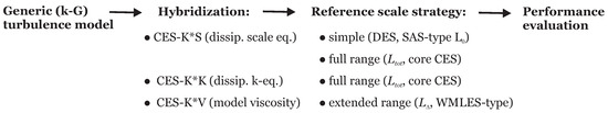
Figure 1.
Overview of the analysis presented. CES refers to continuous eddy simulation; K*S, K*K, and K*V refer to the generic turbulence model used in the different hybridization versions (hybridization in scale equation, k equation, and ).
2. Generic Two-Equation Turbulence Model
As a basis for the following discussion, we introduce first the two-equation turbulence model [2,121]. The model considered is given by the incompressible continuity equation and momentum equation
Here, denotes the filtered Lagrangian time derivative, and the sum convention is used throughout this paper. refers to the component of the spatially filtered velocity. We have here the filtered pressure , is the constant mass density, k is the modeled energy, is the constant kinematic viscosity, and is the rate-of-strain tensor. The modeled viscosity is given by . Here, is a model parameter with a standard value , and L is a characteristic length scale. The latter can be related to the dissipation rate of modeled kinetic energy, or the dissipation time scale , or turbulence frequency by , respectively. We note that RANS and LES approaches differ by different settings of characteristic length scales L in and the different grids applied. For k and , we consider the transport equations
Here, is the production of k, where is the characteristic shear rate. is a constant with standard value , and . In addition we have , where [2] implies . For simplicity we show the diffusion term for high flows, i.e., the contribution of to the diffusivity is neglected. For clarity purposes we do account for , which is usually set equal to unity.
It is relevant to note that the methods presented are applicable to stratified flows if appropriate extensions are considered [116]. There is a need for the addition of a potential temperature equation and the addition of buoyancy and Coriolis terms in the mean flow equations. In regard to the further analysis presented in this paper, it is relevant to note that the analysis of turbulence models is unchanged with the understanding that the buoyancy production has to be added to the shear production P.
There is not only the model [2,121] that is applied to determine the turbulence scale; there is also a large variety of models that are applied instead of the model: models [2,122], models [123,124,125], models [5,9,10,126], models [5,12], and stand-alone models without the k-equation [13,127,128]. To enable the discussion of a large variety of usually applied turbulence models, we generalize the scale equation considered (the ϵ Equation (2b)). Specifically, we follow Umlauf and Burchard [129] by introducing the generic scale variable . Here, m and are any numbers, and is a function of that depends on the model: e.g., we have
The use of the model in conjunction with the definition enables the derivation of the following generic turbulence model:
Here, , , and the following abbreviations are applied:
Three examples for scale equations implied in this way are given in Table 1, where the corresponding and are given in terms of Equation (5). Two relevant observations are the following ones: First, the source terms should not include diffusive turbulent transport terms, leading to the requirement that . We will assume from now on as is usually assumed. Nevertheless, to stress the generality of further developments, we will keep as an adjustable parameter (keeping in mind that turbulence models do not always strictly follow requirements). Second, the appearance of cross-diffusion terms in the dissipation term given by is not in line with turbulence modeling principles. (i) There is no reason to assume that the model has a higher degree of reliability than other two-equation models. By using another turbulence model than the model, we would obtain different cross-diffusion terms in regard to every two-equation turbulence model considered. Thus, these terms simply represent spurious source terms, which should be disregarded. (ii) In addition, the nondimensional is unbounded, and it can be positive or negative. Thus, the inclusion of in the dissipation term may imply random effects. (iii) The strongest argument against the inclusion of is that it prevents the hybridization of the generic model presented below. As argued in the introduction, this fact speaks against physical principles.

Table 1.
Equations for , , and derived from the model.
Based on these arguments we will consider the following generic turbulence model:
Here, and are constants, and . The last expression in Equation (6b) indicates the spirit of this model, the trend toward a production-to-dissipation equilibrium. As pointed out in Appendix A, there are three conditions imposed on this model. In addition to , the log law implies
On top of this there is the constraint . The latter condition is usually not strictly satisfied, but most turbulence models apply settings in line with this requirement.
3. Hybridization Frameworks
The generic turbulence model provides the basis for hybridizations, but there are actually three ways to address this question. A first way is to hybridize dissipation terms in the generic model. A second way is to hybridize the modeled viscosity in the generic turbulence model equation. A third way is the reduction of the generic two-equation model to a one-equation model with corresponding hybridization. Details of these three techniques will be presented in the following section. These results are summarized in Table 2.
Table 2.
Summary of hybrid models obtained, where and . Characteristic-related settings for the reference length scale are given on the right-hand side. Based on , the log-law requirements for CES-K*S, CES-K*K, and CES-K*V are . The last two rows (CES-SAS and CES-DES) describe specific choices of CES-K*S. For the model we have , and for the model we have and , respectively.
3.1. Hybridization of the Generic Two-Equation Model
According to Equation (6), the turbulence model considered is expressed as
In the RANS equations, we have a constant . In contrast to that, is considered to be an adjustable parameter here. As pointed out in the introduction, a rudimentary expectation is a model’s ability to seamlessly cover resolving and modeling flow regimes. However, it requires care with the understanding of the meaning of resolving and modeling flow regimes. Used on appropriate grids, Equation (8) can be used in the resolving mode; the turbulence variables such as L and k become much smaller than in RANS mode in this case. However, a transition between different regimes cannot trivially be accomplished by using Equation (8) on appropriate (fine or coarser) grids in conjunction with . In this case, Equation (8) would operate as an unsteady RANS with a random, uncontrolled inclusion of some resolved motion (which is known to be an inappropriate concept; see LES performed on coarse grids). Consequently, this transition has to be driven by the model itself. The latter can be accomplished by variational analysis that requires the model to ensure a transition between different scaling regimes. As shown in Appendix B, such variational analysis implies
where refers to the modeled reference length scale ratio (no assumption regarding the reference length scale will be made right now). An assumption made in this analysis is the neglect of substantial derivatives and only in regard to the calculation of . This assumption simplifies equations; it was found to be very well justified in previous applications [109,110,119].
The hybridization of the dissipation in the scale equation is not the only option; it is also possible to apply a corresponding hybridization of the dissipation in the k-equation,
where the adjustable hybridization parameter is introduced. By using the same analysis as before (see Appendix B) we obtain
It is remarkable to see that drives the hybridization for the large family of turbulence models considered and for different types of hybridizations. As expected and desired by Rotta [9,10], we find that a length scale () enters the turbulence production–dissipation terms in addition to the time scale .
3.2. Viscosity Hybridization of the Generic Two-Equation Model
Hybridizations of the generic model by modifying dissipation terms in the scale or k equation are not the only options: there is another option focusing on the hybridization of the modeled viscosity . The generic turbulence model equations considered for this case are given by
Here, is a constant as considered before, and the adjustable is introduced. The latter stands for a modification of the modeled viscosity, with the understanding that is used inside the gradient term of turbulent transport terms. As shown in Appendix C by using a corresponding variational analysis as before, we obtain for this case
Here, and refer to any reference state. A significant difference to the hybridizations in terms of and considered before is that fact that scales with instead of the scaling with obtained in regard to and .
3.3. The One-Equation Hybrid Generic Model
The reduction of the generic model to a one-equation model can be obtained as follows (more specifically, we derive first a two-equation model that enables the transition to an one-equation model). This derivation is only meaningful by considering a modeled viscosity equation: ; no other assumption is made,
Here, refers to an adjustable hybridization parameter. According to Equation (A13), is given by
Here, is used again as a non-specified reference scale.
The transition to a one-equation model is described in Appendix D. We obtain in this way
see Equation (A23). An alternative writing is given by Equation (A24),
In these equations, , , and are model parameters. An essential fact is the following: The latter parameters are obtained by model variables including , which has a log-law value of unity. No attempt is made to satisfy log-law requirements via setting . Instead, the log-law requirements are imposed as conditions on model parameters given by and , respectively; see Appendix D.
4. Analysis of Hybridization Strategies
A summary of available modeling frameworks as presented in Section 3 is given in Table 2. The actual hybridization requires a specification of the reference state, in particular the setting of . This is very essential: the range covered by L to variations determines the hybrid range covered by the simulation method. Several possibilities for settings (which depend on the specific modeling framework considered) will be discussed in the following section. An overview of these options is provided in Figure 2. For clarity purposes we only discuss here the implications of settings in regard to Table 2 methods; no further assumptions as usually applied will be made.
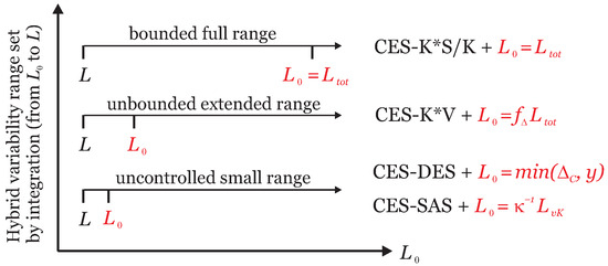
Figure 2.
Functionality range of hybrid RANS-LES methods implied by settings of the reference length scale , which determines the hybrid range covered by the method.
4.1. Simple Empirical Strategies
The first most simple strategy is to follow the DES concept, characterized by a switch of RANS and LES length scales. DES can be applied in a variety of versions. For the following discussion we focus on a comparison with a one-equation modeled viscosity equation (see Equations (16) and (17))
The DES concept is to apply [49]. Here, is the filter width, , and y is the distance from the nearest wall. The constant is given by , where refers to the Kolmogorov constant. Values , e.g., imply . In DES methods, the typical notation applied is , where the characteristic DES constant is introduced. The idea of this approach is to enable the simulation of instationary flow on appropriate grids. In this mode, the model length scale L is much smaller than in RANS mode; L can be of the order of the filter width . Then, there is little variation of ; see the illustration in Figure 2. This means, as given by DES does not allow it to span regimes ranging from total modeling to a total flow resolution: the DES concept is therefore an inappropriate concept to set up seamlessly operating hybrid simulation methods. This conclusion is fully in line with the experience obtained by DES simulations. There is research for about 30 years of how to stabilize the uncontrolled interaction of modeled and resolved flow without any convergence accomplished so far [130].
A second simple strategy (applicable in the CES-K*S framework) is the use of the von Kármán length scale as the reference length scale as applied in SAS methods, where . In the logarithmic flow region we find . A simple way to illustrate the SAS approach is to take reference to Equation (14),
By using and and , the equation can be written as
The typical SAS setting applied is then . Based on the ability of to pick up flow instabilities, reference to a resolving flow regime is included in this way [5]. This approach is successful [5,12,91,92,93,94], but concerns arise from both a theoretical viewpoint [131,132] and with respect to the simulation performance [133]. These issues can be traced back to the concept of not spanning a complete variability range of the model in between fully resolved and fully modeled regimes (see the illustration in Figure 2). Something of interest is the following: there is ambiguity in the SAS approach of how to include the effect of : a linear dependency on the second velocity derivative was proposed first [12], whereas a quadratic formulation has been used later [5]. The analysis presented here confirms the need for a quadratic formulation.
4.2. Unbounded Extended Range
A systematic strategy (applicable in the CES-K*V framework) for introducing such that a variety of resolution regimes is spanned is to match LES scaling with modeling. This concept may be seen to safeguard an LES simulation performed on relatively coarse grids (grids that cannot ensure an appropriate LES resolution). By using , the latter can be accomplished based on [120]
where , and . For a sufficiently small , Equation (21) implies . The relation is simply a consequence of calculating L by integration over the Kolmogorov spectrum [81]. Equation (21) can be simplified by replacing by combined with an appropriate bounding. This leads to
This bounding is relatively well justified; see Figure 3, where is shown.
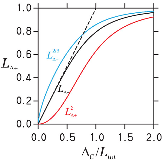
Figure 3.
, , and determined by . We used here the abbreviation . The dashed line shows .
It is of interest to note that this strategy is only meaningful within the CES-K*V concept, which involves scaling with in contrast to the in the other modeling approaches. Hence, we consider
The use of combined with according to Equation (22) and (for simplicity) results in
4.3. Bounded Full Range
The only way to enable a transitioning between fully resolved and fully modeled regimes (applicable in the CES-K*S/K framework) is the identification , where is the total length scale involving both modeled and resolved contributions (see below). This approach can be implemented in CES-K*S,
and CES-K*K models,
According to Equation (9), we have here . In contrast to the notation applied before, we apply here , where . Correspondingly, we switch from to , where is the RANS value of . By definition we have ; refers to complete flow resolution, whereas refers to complete modeling. The mechanism of variations between the RANS state and LES can be seen by considering Equation (26). implies that . An increase in via variations increases the dissipation of k and it decreases k. For we have . Then, the production–dissipation terms of both the k and G equations are driven by , and the source terms finally disappear, leading to a zero modeled viscosity (the DNS limit). The computational methods obtained in this way are referred to as CES.
The difference between CES as presented here to usually applied RANS methods is the appearance of the resolution indicator . The modeled contribution is calculated by (the brackets refer to averaging in time). The total length scale is calculated correspondingly by . Here, is the sum of modeled and resolved contributions, where the resolved contribution is calculated by
Correspondingly, is the sum of modeled and resolved contributions, , where
Both and are calculated on the fly (during the simulation) by using Equations (27) and (28) to process the resolved fluctuations produced by the model. It is of interest to note that is related to the corresponding kinetic energy ratio by , where . Away from walls, represents a good approximation which implies .
5. Performance of Hybridization Strategies
To further scrutinize the suitability of hybridization strategies, we turn now to illustrations of their flow simulation performance. This discussion will focus on two complex high- wall-bounded turbulent flows that include flow separation: flow over periodic hills [134,135] and flow over a NASA wall-mounted hump [136]. For both of these flows, applications of the simulation methods under consideration are available.
An illustration of the periodic hill flow considered is given in Figure 4 [119]. This flow is a channel flow involving periodic restrictions. The flow, which is used a lot for the evaluation of turbulence models [6], involves features such as separation, recirculation, and natural reattachment [134,135]. Specifically, we consider this flow at the highest K for which experimental data for model evaluation are still available [119,134,135]. The NASA wall-mounted hump flow is illustrated in Figure 5. Seifert and Pack [136] developed the wall-mounted hump model to investigate unsteady flow separation, reattachment, and flow control at a high Reynolds number K based on the chord length c and freestream velocity . Here, is the dynamic viscosity, and the subscript abbreviation indicates the reference freestream conditions, which are determined at the axial point . The model reflects the upper surface of a 20-thick Glauert-Goldschmied airfoil that was originally designed for flow control purposes in the early twentieth century. As a benchmark for comparison, we used the experiment conducted by Greenblatt et al. [137] without flow control. This benchmark case has been extensively documented on the NASA Langley Research Center’s Turbulence Modeling Resource webpage and has been widely used for evaluating different turbulence modeling techniques, as discussed in the 2004 CFD Validation Workshop. We see in Figure 5 a strongly convex region just before the trailing edge, which induces flow separation.
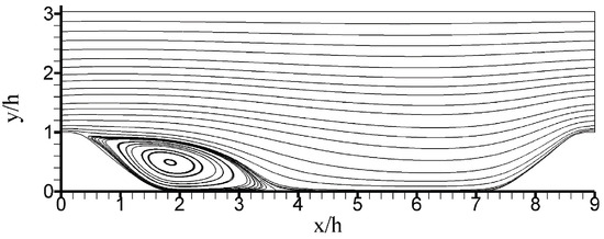
Figure 4.
Velocity streamlines seen in periodic hill flows: results obtained by continuous eddy simulation at = 37,000. Reprinted with permission from Ref. [119]. Copyright 2020 AIP Publishing.
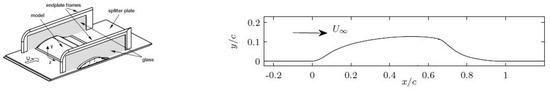
Figure 5.
Wall-mounted hump geometry. (left) Experimental setup [136]; (right) 2-D computational layout.
The computational methods considered in this section are presented in Table 3. For reasons explained in Section 4, the main focus will be on methods having the potential to systematically cover wide hybridization regimes (methods described in Section 4.2 and Section 4.3). In particular, CES-K*V has not been strictly applied so far. However, there is a version of it (referred to as the grid-adaptive simulation (GAS) method), which is very similar to CES-K*V. The GAS approach has been applied in Refs. [133,138,139] with two significant differences to CES-K*V: instead of in Equation (24), these authors applied , and the bounding has been replaced by L,
The latter [i.e., ] is a representation of the modeled-to-total k ratio in difference to the squared modeled-to-total L ratio derived here by variational analysis. As shown in Figure 3, such a modification certainly can affect the performance of simulations. An attractive feature of this approach is its computational simplicity; simulations can be performed without any need to calculate additional variables (like ). The disadvantage is the following: modeling variables such as k and L do not represent RANS variables in partially resolving simulations, i.e., the concept considered cannot provide a transition between fully resolved and fully modeled regimes.
Table 3.
Computational methods involved in performance analysis. Here, SST refers to the shear–stress transport (SST) turbulence model [140], used as the RANS baseline model.
5.1. Simple Empirical Strategies
DES and SAS face significant conceptual shortcomings; see the discussion in Section 4.1. Therefore, the DES and SAS methods will only be briefly discussed as part of the discussion of GAS methods in the next subsection. It is worth noting that the DES and SAS results discussed here were obtained by the same simulating settings as used in regard to GAS methods [133].
With regard to the periodic hill flow, DES and SAS results for reattachment point predictions are reported in Table 4. Such reattachment point predictions represent a valuable criterion of how well simulation methods can deal with separation zone characteristics. It may be seen that both SAS-SST and DDES-SST provide rather inaccurate predictions. Used on the same grid as RANS-SST, they behave basically like RANS (there is no advantage of using a hybrid method).
Table 4.
Reattachment point locations and errors to experiments for several methods. Left: periodic hill flow at K. In experiments, the reattachment point is reported as [134]. Right: NASA hump flow at K. The reattachment point is reported as [137].
With regard to the NASA hump flow, the corresponding DES and SAS results for reattachment point predictions are also reported in Table 4. Although the results are less drastic, the message is pretty much the same as obtained for the hill flow case. In particular, there is no substantial advantage of SAS-SST and DDES-SST compared to RANS-SST. More specifically, the performance of DDES-SST is much worse than the corresponding RANS-SST prediction. The SAS-SST and DDES-SST pressure coefficient () and skin friction coefficients () distributions are shown in Figure 6; the SAS-SST and DDES-SST mean velocity predictions are shown in Figure 7. The unsatisfactory performance of SAS-SST and DDES-SST with respect to these predictions, in particular DDES-SST, is clearly visible. The corresponding SAS-SST and DDES-SST predictions of the total Reynolds stress contour plots (not shown here) reveal that SAS-SST and DDES-SST incorrectly characterize the overall flow structure [133].
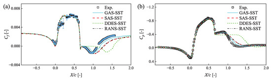
Figure 6.
NASA hump flow, (a) skin friction (), and (b) pressure coefficient () distributions obtained by GAS-SST on the 0.77M grid compared to other results [133] [taken from Wang et al. [133] with permission].
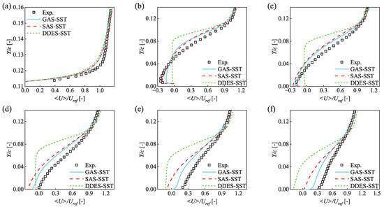
Figure 7.
NASA hump flow; mean velocity profiles obtained by GAS-SST on the 0.77M grid compared to other results [133] [taken from Wang et al. [133] with permission]. The positions from the left to the right and from (a–f) are , respectively.
5.2. Unbounded Extended Range
With regard to the periodic hill flow, the GAS-SST predictions show a very different picture. The reattachment point predictions are reported in Table 4. Overall, the results are good. Nevertheless, in contrast to expectations, we observe that a grid refinement implies a systematic increase in the error. Similarly, a grid refinement leads to slightly less accurate predictions of the pressure coefficient distribution (not shown here). Velocity and Reynolds stress predictions on the coarsest grid show a very good agreement with measurements (not shown here).
With regard to the NASA hump flow, GAS-SST reattachment point predictions are also reported in Table 4. The error is relatively small and unaffected by grid refinement. GAS-SST skin friction () and pressure coefficient () distributions are shown in Figure 6. The results show significant improvements compared to SAS-SST, DDES-SST, and RANS-SST. Nevertheless, the double-peak structure of the distribution is not well reflected and is no different to RANS-SST. The corresponding mean velocity profiles are shown in Figure 7. Overall, there is a reasonable agreement with experimental results, although the profiles at cannot be seen to be accurate. The grid effect on these results is not reported. The Reynolds stresses are presented reasonably well. Contour plots of total Reynolds stress (not shown here) also show that GAS-SSTS describes the overall flow structure really well compared to experimental results and are much improved compared to SAS-SST and DDES-SST [133].
5.3. Bounded Full Range
In regard to periodic hill flows, the CES-K*K version applied (CES-KOKU, see Table 3) shows an almost perfect prediction of the reattachment point, even the use of a very coarse (0.12M) grid provides excellent reattachment point predictions (see Table 4). A thorough evaluation of the model performance for this flow can be found elsewhere [119]. A significant range of ( K) and a variety of coarse and finer grids (, , and involving 500 K, 250 K, and 120 K grid points, respectively) were considered. In particular, these simulations cover the whole range of simulations under almost resolving and almost completely modeled regimes. These studies reveal an excellent ability of this model to represent the characteristics of the recirculation zone, the structure of the velocity field, and the Reynolds stresses.
In regard to the NASA hump flow, a significant range of (M) and a variety of coarse and finer grids were considered, including a grid with 1.7M grid points and a grid with 3.9M grid points. The reattachment point predictions of the CES-K*S version applied (CES-KOS, see Table 3) are also shown in Table 4. The results are excellent; there are errors of 0.3% and 0% on the and grids, respectively, which is even much below the error of GAS-SST. An example of CES advantages is given in Figure 8 in regard to comparisons with WRLES and WMLES [111]. We see that all methods involved show a reasonable agreement with the experimental pressure coefficient profiles. Figure 8 also shows the mean skin friction coefficient obtained by CES-KOS, WMLES, and WRLES simulations, demonstrating their agreement with experimental values. In the separation zone, from , WRLES underpredicts the skin friction coefficient, while WMLES overestimates the actual peak. In regard to post-reattachment, however, the profiles of WRLES and CES-KOS match relatively well, despite using different frameworks, mesh sizes, and grid resolutions. In regard to GAS-SST, we see that the CES-K*S version applied represents the peak structure better than GAS-SST. Figure 9 shows corresponding mean velocity profiles. The conclusion is that the CES-K*S version applied provides predictions that are equivalent to or better than WRLES, better than WMLES, and better than GAS-SST.
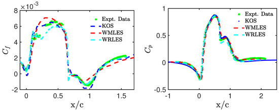
Figure 8.
NASA hump flow, CES-KOS, WMLES [142], and WRLES [143,144] simulation results on the grid at K: skin-friction () and pressure () coefficients [111].
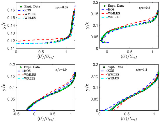
Figure 9.
CES-KOS, WMLES [142], and WRLES [143,144] simulation results on the grid at K: Mean velocity profiles [111].
6. Conclusions
This paper presents an analysis of strategies for the design of seamlessly resolving turbulent flow simulations. The basis for this study is a generic two-equation turbulence model which covers all usually applied two-equation turbulence models like or models. Technically, there are two new ingredients in this approach. First, three basic hybridization frameworks are introduced for this wide class of turbulence models, which are referred to as CES-K*S (hybridization of dissipation in scale equation), CES-K*K (hybridization of dissipation in k equation), and CES-K*V (hybridization of modeled viscosity). The results obtained are based on exact variational analysis. The second technical novelty is the consideration of a flexible hybridization (related to the specification of the reference length scale ), which can be adjusted to several objectives. A first strategy (the simple empirical strategy) is the specification of according to DES-type and SAS-type models. A second strategy (the unbounded extended range strategy) is to take explicit reference to LES scaling in terms of the filter width . A third strategy (the bounded, full-range strategy) is to take reference to the total (RANS type) variables. As illustrated in Figure 2, these three strategies differ significantly with respect to computational requirements and their ability to cover various simulation regimes.
Relevant conclusions presented here can be summarized as follows:
- Turbulence modeling. An essential ingredient of turbulence models is a scale equation, e.g., an or equation. There is no theoretical basis for such an equation; these equations are designed by taking reference to empirical arguments. There exists a huge variety of such equations: the model [2,121], models [2,122], models [123,124,125], models [5,9,10,126], models [5,12], and stand-alone models without a k-equation [13,127,128]. On top of that, a variety of equation structures (including or excluding cross-diffusion terms) is applied. The analysis presented here cannot provide strict guideline for further developments, but it leads to very valuable conclusions. First, the requirement for turbulence models to be applicable to various scaling regimes excludes the inclusion of cross-diffusion terms, which prohibits the hybridization of equations. Second, the diffusivities of the k and scale equations (e.g., the and applied) should be the same. Third, the analysis presented clarifies the structure of dissipation terms; it provides corresponding evidence that is missing in SAS and DES approaches.
- Usually applied hybrid RANS-LES. Based on the fundamental conceptual shortcomings of RANS and LES (to often provide unreliable predictions of separated turbulent flows or to be inapplicable to very high- flows seen in reality because resolution requirements cannot be met), the use of hybrid RANS-LES is the no-alternative approach to deal with these problems. Most hybrid RANS-LES applications are performed with DES-type or WMLES-type models. WMLES is known to be relatively inaccurate [6,110,111]; explicit evidence for this view is provided by the discussions in Section 5. In addition, WMLES faces significant uncertainty of predictions caused by different ways to combine RANS and LES elements in WMLES equations. The situation is different in regard to DES. There is research over decades hoping to improve DES predictions by empirical model improvements combined with variations of how DES is used. For the first time, this paper provides explicit mathematical evidence that DES cannot systematically span a range of modeled-to-resolved flow regimes because of the scaling applied (the setting of ). As specified in Figure 2, DES only triggers uncontrolled instabilities. This is often helpful, but is no guarantee for systematic improvements of simulation results compared to RANS. As shown here, the same issue applies to SAS. The flow simulation results presented in Section 5 fully confirm this view.
- Optimal solution: core CES: A way to overcome these problems is the use of the full-range strategy, which is equivalent to CES methods that apply to explicitly drive the hybrid model in between fully modeled (RANS) and fully resolved (LES) regimes. Applications of this approach [110,111,119] demonstrate an impressive ability of this approach to provide very good flow predictions at relatively low computational cost. A specific feature of CES is its well balanced predictive ability, in contrast to the DES and WMLES methods that can provide some flow characteristics well at the cost of other flow characteristics. Comparisons with WRLES and WMLES results (see, e.g., the comparisons presented in Section 5) show that CES performs clearly better than WMLES and at least as good or better than WRLES at a small fraction of the WRLES cost. It is essential to note that CES methods include via their own flow resolution indicator in contrast to LES methods. This matters in regard to the known difficulty of assessing the resolution ability of LES [24,25]. It is also worth mentioning that the methods presented here (based on the generic model consideration) enable the use of LES in conjunction with a variety of turbulence models that may be considered according to specific requirements.
- Interesting option: WMLES-type CES. In contrast to the usually applied hybrid methods, the CES core methods require the explicit calculation of by processing statistics of resolved motion. Currently available experience shows that this adds only a little fraction to computational costs, but it requires corresponding computational code modifications. An interesting alternative pointed out here is the use of the unbounded extended range strategy, which takes explicitly reference to LES scaling in terms of the filter width . In this way, the involvement of additional simulation ingredients (like ) can be avoided. This concept (which represents a version of consistently formulated WMLES) may be seen to safeguard an LES simulation performed on relatively coarse grids (grids that cannot ensure an appropriate LES resolution). Nevertheless, because of the reference scaling applied, there is no guarantee that this concept works well in regimes on coarse grids, well away from the LES regime. A variant of using this approach has been discussed here by taking reference to GAS simulation results; see Section 5. The results are much better than the corresponding RANS, DES, and SAS results, but not as good as the CES results. It is worth noting that the GAS concept differs from the corresponding result obtained here by variational analysis by applying, for example, an inaccurate scaling with (see the discussion related to Equation (29)).
Funding
This research received no external funding.
Data Availability Statement
Data are contained within the article.
Acknowledgments
I would like to acknowledge support from the National Science Foundation (AGS, Grant No. 2137351, with N. Anderson as Technical Officer). This work was supported by Wyoming NASA Space Grant Consortium (NASA Grant No. 80NSSC20M0113) and the University of Wyoming School of Computing (Wyoming Innovation Partnership grant).
Conflicts of Interest
The author declares no conflict of interest.
Appendix A. Constraints on Generic Model Parameters
By neglecting substantial derivatives, the generic model equations considered are expressed as
where . The log law is accounted for by , where refers to the friction velocity, is the von Kármán constant, and y is the wall distance. The first equation is satisfied by the constant , which implies ; this means . With the help of the relations for k and S that are obtained, the latter relation implies . The combination of these expressions provides a length scale and . Consistency with logarithmic boundary layer observations leads to a first constraint on model parameters given by .
To take advantage of Equation (A1b), we need to calculate . Based on the definition of G, we have , i.e., in the log-law region. The latter implies
The use of this expression in Equation (A1b) in conjunction with leads then to the second constraint on generic model parameters given by
Another model parameter requirement arises as follows. Based on the definition of we find for the turbulence length scale the equation
Let us consider the model’s applicability to homogeneous turbulent shear flow. By using the corresponding transport equations for k and G, we obtain the equation
This relation leads to the third constraint , because homogeneous shear cannot determine a length scale [129].
Appendix B. Hybridization of the Generic Two-Equation Model
The transport equations considered is expressed as
In the RANS equations, we have a constant . In contrast to that, is considered to be an adjustable parameter here. Only in regard to the calculation of here do we neglect the substantial derivatives and as follows. This assumption simplifies the presentation, and it was found to be very well justified in previous applications. We will also assume that the relative variations and are invariant in space and time. This assumption is no restriction at all; it stabilizes simulations through a seamless resolution of differently resolved flow regions. We introduce, then, a hybridization error as a residual of the G equation,
where the k equation is used to replace P in the previous expression. The multiplication of the latter relation with results in
where is applied. According to the assumptions made about energy partitions, we find in the first order of variations the relations
Hence, the variation of the last two terms in Equation (A8) disappears because of
Accordingly, the variation of Equation (A8) leads to
An extremal error is determined by a zero first variation (a zero bracket term),
This equation can be integrated from a reference state (with variables and ) to a state with a certain level of resolved motion, . The result is
where refers to the modeled to reference length scale ratio.
An alternative to the hybridization of the scale equation is a corresponding hybridization applied in the k-equation,
where the adjustable hybridization parameter is introduced. By following the same hybridization approach as used before, we find the hybridization error to be given by
where the k equation is used to replace P in the previous expression. The comparison with Equation (A7) reveals the relationship . In combination with , the latter implies
Appendix C. Viscosity Hybridization of the Generic Two-Equation Model
The transport equations considered is expressed as
Here, is a constant as considered before, and the adjustable is introduced. The latter stands for a modification of the modeled viscosity, with the understanding that is used inside the gradient term of turbulent transport terms. In correspondence with Equation (A7), the error (divided by ) reads
where the k-equation is used to replace P. The variation of the last two term vanishes; see Equation (A10). Combined with , a zero first-order derivative implies
The latter relation can be also written as . This equation can be integrated from a reference state (indicated by the subscript 0) to a state with a certain level of resolved motion, , which leads to
Appendix D. The One-Equation Hybrid Generic Model
The transition to a one-equation hybrid generic model requires a closure for k. This can be accomplished as follows. By using the definitions and , Equation (14b) can also be written as
We introduce . The latter variable represents the ratio of two quadratic length scales, and ; this means . In the log layer we have , which implies . Then, Equation (A21) reads as
where is applied. We introduce two parameters: and , which results in
With the help of , which means or , we can rewrite the second term as
where is introduced. It is worth noting that both Equations (A23) and (A24) can satisfy log-law requirements. Based on , and , the log-law requirement for Equation (A23) reads as
Correspondingly, the log-law requirement for Equation (A24) is given by
where is taken into account.
References
- Kolmogorov, A.N. Equations of turbulent motion of an incompressible fluid. Izv. Akad. Nauk SSR Seria Fiz. 1942, 6, 56–58. [Google Scholar]
- Wilcox, D.C. Turbulence Modeling for CFD, 2nd ed.; DCW Industries: La Canada Flintridge, CA, USA, 1998. [Google Scholar]
- Hanjalić, K. Advanced turbulence closure models: A view of current status and future prospects. Int. J. Heat Fluid Flow 1994, 15, 178–203. [Google Scholar]
- Hanjalić, K. Will RANS survive LES?: A view of perspectives. ASME J. Fluids Eng. 2005, 127, 831–839. [Google Scholar] [CrossRef]
- Menter, F.R.; Egorov, Y. The scale-adaptive simulation method for unsteady turbulent flow prediction: Part 1: Theory and model description. Flow Turbul. Combust. 2010, 78, 113–138. [Google Scholar] [CrossRef]
- Heinz, S. A review of hybrid RANS-LES methods for turbulent flows: Concepts and applications. Prog. Aerosp. Sci. 2020, 114, 100597. [Google Scholar]
- Asinari, P.; Fasano, M.; Chiavazzo, E. A kinetic perspective on k-ϵ turbulence model and corresponding entropy production. Entropy 2016, 18, 121. [Google Scholar] [CrossRef]
- Bhatnagar, P.L.; Gross, E.P.; Krook, M. A model for collision processes in gases. I. Small amplitude processes in charged and neutral one-component systems. Phys. Rev. 1954, 94, 511–525. [Google Scholar] [CrossRef]
- Rotta, J.C. Über eine Methode zur Berechnung Turbulenter Scherströmungen. Aerodyn. Vers. Gott. 1968, Rep. 69, A14. [Google Scholar]
- Rotta, J.C. Turbulente Strömumgen; BG Teubner: Stuttgart, Germany, 1972. [Google Scholar]
- Rodi, W. Turbulence modelling for boundary-layer calculations. In Proceedings of the IUTAM Symposium on One Hundred Years of Boundary Layer Research, Göttingen, Germany, 12–14 August 2004; Meier, G., Sreenivasan, K., Eds.; Springer: Berlin/Heidelberg, Germany, 2006; pp. 247–256. [Google Scholar]
- Menter, F.R.; Egorov, Y. Revisiting the turbulent scale equation. In Proceedings of the IUTAM Symposium on One Hundred Years of Boundary Layer Research, Göttingen, Germany, 12–14 August 2004; Meier, G.E.A., Sreenivasan, K.R., Eds.; Springer: Dordrecht, The Netherlands, 2006; pp. 279–290. [Google Scholar]
- Spalart, P.; Allmaras, S. A one-equation turbulence model for aerodynamic flows. La Rech. Aérospatiale 1994, 1, 5–21. [Google Scholar]
- Pope, S.B. Turbulent Flows; Cambridge University Press: Cambridge, UK, 2000. [Google Scholar]
- Sagaut, P. Large Eddy Simulation for Incompressible Flows: An Introduction; Springer: Berlin, Germany, 2002. [Google Scholar]
- Lesieur, M.; Metais, O.; Comte, P. Large-Eddy Simulations of Turbulence; Cambridge University Press: Cambridge, UK, 2005. [Google Scholar]
- Piomelli, U. Large-eddy simulation: Achievements and challenges. Prog. Aerosp. Sci. 1999, 35, 335–362. [Google Scholar] [CrossRef]
- Piomelli, U. Large eddy simulations in 2030 and beyond. Phil. Trans. R. Soc. A 2014, 372, 20130320/1–20130320/23. [Google Scholar] [CrossRef]
- Yang, X.I.A.; Sadique, J.; Mittal, R.; Meneveau, C. Integral wall model for large eddy simulations of wall-bounded turbulent flows. Phys. Fluids 2015, 27, 025112. [Google Scholar] [CrossRef]
- Larsson, J.; Kawai, S.; Bodart, J.; Bermejo-Moreno, I. Large eddy simulation with modeled wall-stress: Recent progress and future directions. Mech. Eng. Rev. 2016, 3, 15-00418. [Google Scholar] [CrossRef]
- Bose, S.T.; Park, G.I. Wall-modeled large-eddy simulation for complex turbulent flows. Annu. Rev. Fluid Mech. 2018, 50, 535–561. [Google Scholar] [CrossRef]
- Yang, X.I.A.; Griffin, K.P. Grid-point and time-step requirements for direct numerical simulation and large-eddy simulation. Phys. Fluids 2021, 33, 015108. [Google Scholar] [CrossRef]
- Toosi, S.; Larsson, J. Towards systematic grid selection in LES: Identifying the optimal spatial resolution by minimizing the solution sensitivity. Comput. Fluids 2020, 201, 104488. [Google Scholar] [CrossRef]
- Davidson, L. Large Eddy Simulations: How to evaluate resolution. Int. J. Heat Fluid Flow 2009, 30, 1016–1025. [Google Scholar] [CrossRef]
- Wurps, H.; Steinfeld, G.; Heinz, S. Grid-resolution requirements for large-eddy simulations of the atmospheric boundary layer. Boundary Layer Meteorol. 2020, 175, 119–201. [Google Scholar] [CrossRef]
- Deardorff, J.W. A numerical study of three-dimensional turbulent channel flow at large Reynolds numbers. J. Fluid Mech. 1970, 41, 453–480. [Google Scholar] [CrossRef]
- Schumann, U. Subgrid scale model for finite difference simulations of turbulent flows in plane channels and annuli. J. Comput. Phys 1975, 18, 376–404. [Google Scholar] [CrossRef]
- Grötzbach, G. Direct numerical and large eddy simulation of turbulent channel flow. Encycl. Fluid Mech. 1987, 6, 1337–1391. [Google Scholar]
- Piomelli, U.; Ferziger, J.; Moin, P. New approximate boundary conditions for large eddy simulations of wall-bounded flows. Phys. Fluids A 1989, 6, 1061–1068. [Google Scholar] [CrossRef]
- Cabot, W.; Moin, P. Approximate wall boundary conditions in the large-eddy simulation of high Reynolds number flow. Flow Turbul. Combust. 1999, 63, 269–291. [Google Scholar] [CrossRef]
- Piomelli, U.; Balaras, E. Wall-layer models for large-eddy simulations. Annu. Rev. Fluid Mech. 2002, 34, 349–374. [Google Scholar] [CrossRef]
- Piomelli, U. Wall-layer models for large-eddy simulations. Prog. Aerosp. Sci. 2008, 44, 437–446. [Google Scholar] [CrossRef]
- Kawai, S.; Larsson, J. Wall-modeling in large eddy simulation: Length scales, grid resolution, and accuracy. Phys. Fluids 2012, 24, 015105. [Google Scholar] [CrossRef]
- Bose, S.T.; Moin, P. A dynamic slip boundary condition for wall-modeled large-eddy simulation. Phys. Fluids 2014, 26, 015104. [Google Scholar] [CrossRef]
- Park, G.I.; Moin, P. An improved dynamic non-equilibrium wall-model for large eddy simulation. Phys. Fluids 2014, 26, 015108. [Google Scholar] [CrossRef]
- Moin, P.; Bodart, J.; Bose, S.; Park, G.I. Wall-modeling in complex turbulent flows. In Advances in Fluid-Structure Interaction, Notes on Numerical Fluid Mechanics and Multidisciplinary Design 133; Braza, M., Bottaro, A., Thompson, M., Eds.; Springer: Cham, Switzerland, 2016; pp. 207–219. [Google Scholar]
- Chen, S.; Xia, Z.; Pei, S.; Wang, J.; Yang, Y.; Xiao, Z.; Shi, Y. Reynolds-stress-constrained large-eddy simulation of wall-bounded turbulent flows. J. Fluid Mech. 2012, 703, 1–28. [Google Scholar] [CrossRef]
- Chen, S.; Chen, Y.; Xia, Z.; Qu, K.; Shi, Y.; Xiao, Z.; Liu, Q.; Cai, Q.; Liu, F.; Lee, C.; et al. Constrained large-eddy simulation and detached eddy simulation of flow past a commercial aircraft at 14 degrees angle of attack. Sci. China Phys. Mech. Astron. 2013, 56, 270–276. [Google Scholar] [CrossRef]
- Xia, Z.; Shi, Y.; Hong, R.; Xiao, Z.; Chen, S. Constrained large-eddy simulation of separated flow in a channel with streamwise-periodic constrictions. J. Turbul. 2013, 14, 1–21. [Google Scholar] [CrossRef]
- Jiang, Z.; Xiao, Z.; Shi, Y.; Chen, S. Constrained large-eddy simulation of wall-bounded compressible turbulent flows. Phys. Fluids 2013, 25, 106102. [Google Scholar] [CrossRef]
- Hong, R.; Xia, Z.; Shi, Y.; Xiao, Z.; Chen, S. Constrained large-eddy simulation of compressible flow past a circular cylinder. Commun. Comput. Phys. 2014, 15, 388–421. [Google Scholar] [CrossRef]
- Zhao, Y.; Xia, Z.; Shi, Y.; Xiao, Z.; Chen, S. Constrained large-eddy simulation of laminar-turbulent transition in channel flow. Phys. Fluids 2014, 26, 095103. [Google Scholar] [CrossRef]
- Xua, Q.; Yang, Y. Reynolds stress constrained large eddy simulation of separation flows in a U-duct. J. Propul. Power Res. 2014, 3, 49–58. [Google Scholar] [CrossRef]
- Xia, Z.; Xiao, Z.; Shi, Y.; Chen, S. Constrained large-eddy simulation for aerodynamics. In Progress in Hybrid RANS-LES Modelling, Notes on Numerical Fluid Mechanics and Multidisciplinary Design 130; Girimaji, S., Haase, W., Peng, S.H., Schwamborn, D., Eds.; Springer: Cham, Switzerland, 2015; pp. 239–254. [Google Scholar]
- Jiang, Z.; Xiao, Z.; Shi, Y.; Chen, S. Constrained large-eddy simulation of turbulent flow and heat transfer in a stationary ribbed duct. Int. J. Numer. Methods Heat Fluid Flow 2016, 26, 1069–1091. [Google Scholar] [CrossRef]
- Verma, A.; Park, N.; Mahesh, K. A hybrid subgrid-scale model constrained by Reynolds stress. Phys. Fluids 2013, 25, 110805. [Google Scholar] [CrossRef]
- Xiao, Z.; Shi, Y.; Xia, Z.; Chen, S. Comment on ‘A hybrid subgrid-scale model constrained by Reynolds stress’ [Phys. Fluids 25, 110805 (2013)]. Phys. Fluids 2014, 26, 059101. [Google Scholar] [CrossRef]
- Verma, A.; Park, N.; Mahesh, K. Response to Comment on “A hybrid subgrid-scale model constrained by Reynolds stress” [Phys. Fluids 26, 059101 (2014)]. Phys. Fluids 2014, 26, 059102. [Google Scholar] [CrossRef]
- Spalart, P.R.; Jou, W.H.; Strelets, M.; Allmaras, S.R. Comments on the feasibility of LES for wings, and on a hybrid RANS/LES approach. In Advances in DNS/LES; Liu, C., Liu, Z., Eds.; Greyden Press: Columbus, OH, USA, 1997; pp. 137–147. [Google Scholar]
- Travin, A.; Shur, M.L.; Strelets, M.; Spalart, P. Detached-eddy simulations past a circular cylinder. Flow Turbul. Combust. 1999, 63, 113–138. [Google Scholar] [CrossRef]
- Spalart, P.R. Strategies for turbulence modelling and simulations. Int. J. Heat Fluid Flow 2000, 21, 252–263. [Google Scholar] [CrossRef]
- Strelets, M. Detached eddy simulation of massively separated flows. In Proceedings of the 39th AIAA Aerospace Sciences Meeting and Exhibit, Reno, NV, USA, 8–11 January 2001; AIAA Paper 01-0879. pp. 1–18. [Google Scholar]
- Travin, A.; Shur, M.L. Physical and numerical upgrades in the detached-eddy simulation of complex turbulent flows. In Advances in LES of Complex Flows; Friedrich, R., Rodi, W., Eds.; Kluwer Academic Publishers: Dordrecht, The Netherlands, 2002; pp. 239–254. [Google Scholar]
- Menter, F.R.; Kuntz, M.; Langtry, R. Ten years of industrial experience with SST turbulence model. Turbul. Heat Mass Transf. 2003, 4, 625–632. [Google Scholar]
- Spalart, P.R.; Deck, S.; Shur, M.L.; Squires, K.D.; Strelets, M.K.; Travin, A. A new version of detached-eddy simulation, resistant to ambiguous grid densities. Theor. Comput. Fluid Dyn. 2006, 20, 181–195. [Google Scholar] [CrossRef]
- Shur, M.L.; Spalart, P.R.; Strelets, M.K.; Travin, A. A hybrid RANS-LES approach with delayed-DES and wall-modelled LES capabilities. Int. J. Heat Fluid Flow 2008, 29, 1638–1649. [Google Scholar] [CrossRef]
- Spalart, P.R. Detached-eddy simulation. Annu. Rev. Fluid Mech. 2009, 41, 181–202. [Google Scholar] [CrossRef]
- Mockett, C.; Fuchs, M.; Thiele, F. Progress in DES for wall-modelled LES of complex internal flows. Comput. Fluids 2012, 65, 44–55. [Google Scholar] [CrossRef]
- Friess, C.; Manceau, R.; Gatski, T.B. Toward an equivalence criterion for hybrid RANS/LES methods. Comput. Fluids 2015, 122, 233–246. [Google Scholar] [CrossRef]
- Chaouat, B. The state of the art of hybrid RANS/LES modeling for the simulation of turbulent flows. Flow Turbul. Combust. 2017, 99, 279–327. [Google Scholar] [CrossRef]
- Menter, F.; Hüppe, A.; Matyushenko, A.; Kolmogorov, D. An overview of hybrid RANS–LES models developed for industrial CFD. Appl. Sci. 2021, 11, 2459. [Google Scholar] [CrossRef]
- Heinz, S. Unified turbulence models for LES and RANS, FDF and PDF simulations. Theoret. Comput. Fluid Dynam. 2007, 21, 99–118. [Google Scholar] [CrossRef]
- Heinz, S. Realizability of dynamic subgrid-scale stress models via stochastic analysis. Monte Carlo Methods Applic. 2008, 14, 311–329. [Google Scholar] [CrossRef]
- Heinz, S.; Gopalan, H. Realizable versus non-realizable dynamic subgrid-scale stress models. Phys. Fluids 2012, 24, 115105. [Google Scholar] [CrossRef]
- Gopalan, H.; Heinz, S.; Stöllinger, M. A unified RANS-LES model: Computational development, accuracy and cost. J. Comput. Phys. 2013, 249, 249–279. [Google Scholar] [CrossRef]
- Mokhtarpoor, R.; Heinz, S.; Stoellinger, M. Dynamic unified RANS-LES simulations of high Reynolds number separated flows. Phys. Fluids 2016, 28, 095101. [Google Scholar] [CrossRef]
- Mokhtarpoor, R.; Heinz, S. Dynamic large eddy simulation: Stability via realizability. Phys. Fluids 2017, 29, 105104. [Google Scholar] [CrossRef]
- Girimaji, S.; Srinivasan, R.; Jeong, E. PANS turbulence for seamless transition between RANS and LES: Fixed-point analysis and preliminary results. In Proceedings of the ASME FEDSM03, Honolulu, HI, USA, 6–11 July 2003; ASME Paper FEDSM2003-45336. pp. 1–9. [Google Scholar]
- Girimaji, S.; Abdol-Hamid, K. Partially averaged Navier Stokes model for turbulence: Implemantation and validation. In Proceedings of the 43rd AIAA Aerospace Sciences Meeting and Exhibit, Reno, NV, USA, 10–13 January 2005; AIAA Paper 05-0502. pp. 1–14. [Google Scholar]
- Girimaji, S. Partially-averaged Navier-Stokes method for turbulence: A Reynolds-averaged Navier-Stokes to direct numerical simulation bridging method. ASME J. Appl. Mech. 2006, 73, 413–421. [Google Scholar] [CrossRef]
- Girimaji, S.; Jeong, E.; Srinivasan, R. Partially averaged Navier-Stokes method for turbulence: Fixed point analysis and comparisons with unsteady partially averaged Navier-Stokes. ASME J. Appl. Mech. 2006, 73, 422–429. [Google Scholar] [CrossRef]
- Lakshmipathy, S.; Girimaji, S.S. Extension of Boussinesq turbulence constitutive relation for bridging methods. J. Turbul. 2007, 8, 1–20. [Google Scholar] [CrossRef]
- Frendi, A.; Tosh, A.; Girimaji, S. Flow past a backward-facing step: Comparison of PANS, DES and URANS results with experiments. Int. J. Comput. Methods Eng. Sci. Mech. 2007, 8, 23–38. [Google Scholar] [CrossRef]
- Lakshmipathy, S.; Girimaji, S.S. Partially averaged Navier-Stokes (PANS) method for turbulence simulations: Flow past a circular cylinder. ASME J. Fluids Eng. 2010, 132, 121202/1–121202/9. [Google Scholar] [CrossRef]
- Jeong, E.; Girimaji, S.S. Partially averaged Navier–Stokes (PANS) method for turbulence simulations: Flow past a square cylinder. ASME J. Fluids Eng. 2010, 132, 121203/1–121203/11. [Google Scholar] [CrossRef]
- Basara, B.; Krajnovic, S.; Girimaji, S.S.; Pavlovic, Z. Near-wall formulation of the partially averaged Navier-Stokes turbulence model. AIAA J. 2011, 42, 2627–2636. [Google Scholar] [CrossRef]
- Krajnovic, S.; Lárusson, R.; Basara, B. Superiority of PANS compared to LES in predicting a rudimentary landing gear flow with affordable meshes. Int. J. Heat Fluid Flow 2012, 37, 109–122. [Google Scholar] [CrossRef]
- Foroutan, H.; Yavuzkurt, S. A partially averaged Navier Stokes model for the simulation of turbulent swirling flow with vortex breakdown. Int. J. Heat Fluid Flow 2014, 50, 402–416. [Google Scholar] [CrossRef]
- Drikakis, D.; Sofos, F. Can artificial intelligence accelerate fluid mechanics research? Fluids 2023, 8, 212. [Google Scholar] [CrossRef]
- Schiestel, R.; Dejoan, A. Towards a new partially integrated transport model for coarse grid and unsteady turbulent flow simulations. Theor. Comput. Fluid Dyn. 2005, 18, 443–468. [Google Scholar] [CrossRef]
- Chaouat, B.; Schiestel, R. A new partially integrated transport model for subgrid-scale stresses and dissipation rate for turbulent developing flows. Phys. Fluids 2005, 17, 065106. [Google Scholar] [CrossRef]
- Chaouat, B.; Schiestel, R. From single-scale turbulence models to multiple-scale and subgrid-scale models by Fourier transform. Theor. Comput. Fluid Dyn. 2007, 21, 201–229. [Google Scholar] [CrossRef]
- Befeno, I.; Schiestel, R. Non-equilibrium mixing of turbulence scales using a continuous hybrid RANS/LES approach: Application to the shearless mixing layer. Flow Turbul. Combust. 2007, 78, 129–151. [Google Scholar] [CrossRef]
- Chaouat, B.; Schiestel, R. Progress in subgrid-scale transport modelling for continuous hybrid nonzonal RANS/LES simulations. Int. J. Heat Fluid Flow 2009, 30, 602–616. [Google Scholar] [CrossRef]
- Chaouat, B. Subfilter-scale transport model for hybrid RANS/LES simulations applied to a complex bounded flow. J. Turbul. 2010, 11, N51. [Google Scholar] [CrossRef]
- Chaouat, B. Simulation of turbulent rotating flows using a subfilter scale stress model derived from the partially integrated transport modeling method. Phys. Fluids 2012, 24, 045108. [Google Scholar] [CrossRef]
- Chaouat, B.; Schiestel, R. Analytical insights into the partially integrated transport modeling method for hybrid Reynolds averaged Navier-Stokes equations-large eddy simulations of turbulent flows. Phys. Fluids 2012, 24, 085106. [Google Scholar] [CrossRef]
- Chaouat, B.; Schiestel, R. Partially integrated transport modeling method for turbulence simulation with variable filters. Phys. Fluids 2013, 25, 125102. [Google Scholar] [CrossRef]
- Chaouat, B.; Schiestel, R. Hybrid RANS-LES simulations of the turbulent flow over periodic hills at high Reynolds number using the PITM method. Comput. Fluids 2013, 84, 279–300. [Google Scholar] [CrossRef]
- Chaouat, B. Application of the PITM method using inlet synthetic turbulence generation for the simulation of the turbulent flow in a small axisymmetric contraction. Flow Turbul. Combust. 2017, 98, 987–1024. [Google Scholar] [CrossRef]
- Menter, F.R.; Kuntz, M.; Bender, R. A scale-adaptive simulation model for turbulent flow predictions. In Proceedings of the 41st AIAA Aerospace Sciences Meeting and Exhibit, Reno, NV, USA, 6–9 January 2003; AIAA Paper 03-0767. pp. 1–12. [Google Scholar]
- Menter, F.R.; Egorov, Y. A scale-adaptive simulation model using two-equation models. In Proceedings of the 43rd AIAA Aerospace Sciences Meeting and Exhibit, Reno, NV, USA, 10–13 January 2005; AIAA Paper 05-1095. pp. 1–13. [Google Scholar]
- Menter, F.R.; Egorov, Y. The scale-adaptive simulation method for unsteady turbulent flow prediction: Part 2: Application to complex flows. Flow Turbul. Combust. 2010, 78, 139–165. [Google Scholar]
- Jakirlić, S.; Maduta, R. Extending the bounds of "steady" RANS closures: Toward an instability-sensitive Reynolds stress model. Int. J. Heat Fluid Flow 2015, 51, 175–194. [Google Scholar] [CrossRef]
- Wyngaard, J.C. Toward numerical modeling in the “Terra Incognita”. J. Atmos. Sci. 2004, 61, 1816–1826. [Google Scholar] [CrossRef]
- Juliano, T.W.; Kosović, B.; Jiménez, P.A.; Eghdami, M.; Haupt, S.E.; Martilli, A. “Gray Zone” simulations using a three-dimensional planetary boundary layer parameterization in the Weather Research and Forecasting Model. Mon. Weather Rev. 2022, 150, 1585–1619. [Google Scholar] [CrossRef]
- Heinz, S.; Heinz, J.; Brant, J.A. Mass transport in membrane systems: Flow regime identification by Fourier analysis. Fluids 2022, 7, 369. [Google Scholar] [CrossRef]
- Heinz, S. The potential of machine learning methods for separated turbulent flow simulations: Classical versus dynamic methods. Fluids 2024, 9, 278. [Google Scholar] [CrossRef]
- Yakhot, V.; Orszag, S.A. Renormalization group analysis of turbulence. I. Basic theory. J. Sci. Comput. 1986, 1, 3–51. [Google Scholar] [CrossRef]
- Yakhot, V.; Orszag, S.A.; Thangam, S.; Gatski, T.B.; Speziale, C.G. Development of turbulence models for shear flows by a double expansion technique. Phys. Fluids A Fluid Dyn. 1992, 4, 1510–1520. [Google Scholar] [CrossRef]
- Nagano, Y.; Itazu, Y. Renormalization group theory for turbulence: Assessment of the Yakhot-Orszag-Smith theory. Fluid Dyn. Res. 1997, 20, 157–172. [Google Scholar] [CrossRef]
- Zhou, Y. Renormalization group theory for fluid and plasma turbulence. Phys. Rep. 2010, 488, 1–49. [Google Scholar]
- Sadiki, A.; Bauer, W.; Hutter, K. Thermodynamically consistent coefficient calibration in nonlinear and anisotropic closure models for turbulence. Contin. Mech. Therm. 2000, 12, 131–149. [Google Scholar] [CrossRef]
- Sadiki, A.; Hutter, K. On Thermodynamics of Turbulence: Development of First Order Closure Models and Critical Evaluation of Existing Models. J. Non-Equil. Thermodyn. 2000, 25, 131. [Google Scholar] [CrossRef]
- Shih, T.H.; Liou, W.W.; Shabbir, A.; Yang, Z.; Zhu, J. A new k-ϵ eddy viscosity model for high reynolds number turbulent flows. Comput. Fluids 1995, 24, 227–238. [Google Scholar] [CrossRef]
- Shaheed, R.; Mohammadian, A.; Kheirkhah Gildeh, H. A comparison of standard k–ε and realizable k–ε turbulence models in curved and confluent channels. Environ. Fluid Mech. 2019, 19, 543–568. [Google Scholar] [CrossRef]
- Heinz, S.; Fagbade, A. Evaluation metrics for partially and fully resolving simulations methods for turbulent flows. Int. J. Heat Fluid Flow 2025, 115, 109867. [Google Scholar] [CrossRef]
- Heinz, S. Physically consistent resolving simulations of turbulent flows. Entropy 2024, 26, 1044. [Google Scholar] [CrossRef] [PubMed]
- Fagbade, A.I. Continuous Eddy Simulation for Turbulent Flows. Ph.D. Thesis, University of Wyoming, Laramie, WY, USA, 2024. Available online: https://www.proquest.com/docview/3058393461 (accessed on 1 May 2025).
- Fagbade, A.; Heinz, S. Continuous eddy simulation (CES) of transonic shock-induced flow separation. Appl. Sci. 2024, 14, 2705. [Google Scholar] [CrossRef]
- Fagbade, A.; Heinz, S. Continuous eddy simulation vs. resolution-imposing simulation methods for turbulent flows. Fluids 2024, 9, 22. [Google Scholar] [CrossRef]
- Heinz, S. A mathematical solution to the Computational Fluid Dynamics (CFD) dilemma. Mathematics 2023, 11, 3199. [Google Scholar] [CrossRef]
- Heinz, S. Minimal error partially resolving simulation methods for turbulent flows: A dynamic machine learning approach. Phys. Fluids 2022, 34, 051705. [Google Scholar] [CrossRef]
- Heinz, S. Remarks on energy partitioning control in the PITM hybrid RANS/LES method for the simulation of turbulent flows. Flow Turbul. Combust. 2022, 108, 927–933. [Google Scholar] [CrossRef]
- Heinz, S. From two-equation turbulence models to minimal error resolving simulation methods for complex turbulent flows. Fluids 2022, 7, 368. [Google Scholar] [CrossRef]
- Heinz, S. Theory-based mesoscale to microscale coupling for wind energy applications. Appl. Math. Model. 2021, 98, 563–575. [Google Scholar] [CrossRef]
- Heinz, S. The continuous eddy simulation capability of velocity and scalar probability density function equations for turbulent flows. Phys. Fluids 2021, 33, 025107. [Google Scholar] [CrossRef]
- Heinz, S.; Peinke, J.; Stoevesandt, B. Cutting-edge turbulence simulation methods for wind energy and aerospace problems. Fluids 2021, 6, 288. [Google Scholar] [CrossRef]
- Heinz, S.; Mokhtarpoor, R.; Stoellinger, M.K. Theory-based Reynolds-averaged Navier-Stokes equations with large eddy simulation capability for separated turbulent flow simulations. Phys. Fluids 2020, 32, 065102. [Google Scholar] [CrossRef]
- Heinz, S. The large eddy simulation capability of Reynolds-averaged Navier-Stokes equations: Analytical results. Phys. Fluids 2019, 31, 021702. [Google Scholar] [CrossRef]
- Rodi, W. Examples of calculation methods for flow and mixing in stratified fluids. J. Geophys. Res. Oceans 1987, 92, 5305–5328. [Google Scholar]
- Wilcox, D.C. Reassessment of the scale-determining equation for advanced turbulence models. AIAA J. 1988, 26, 1299–1310. [Google Scholar] [CrossRef]
- Speziale, C.G. On nonlinear kL and k-ϵ models of turbulence. J. Fluid Mech. 1987, 178, 459–475. [Google Scholar] [CrossRef]
- Smith, B. A near wall model for the k-L two equation turbulence model. In Proceedings of the Fluid Dynamics Conference, Colorado Springs, CO, USA, 20–23 June 1994; AIAA Paper 94-2386. pp. 1–9. [Google Scholar]
- Goldberg, U.; Chakravarthy, S. A kL turbulence closure for wall-bounded flows. In Proceedings of the 35th AIAA Fluid Dynamics Conference and Exhibit, Toronto, ON, Canada, 6–9 June 2005; AIAA Paper 05-4638. pp. 1–11. [Google Scholar]
- Mellor, G.L.; Yamada, T. Development of a turbulence closure model for geophysical fluid problems. Rev. Geophys. 1982, 20, 851–875. [Google Scholar] [CrossRef]
- Wray, T.J.; Agarwal, R.K. Application of new one-equation turbulence model to computations of separated flows. AIAA J. 2014, 52, 1325–1330. [Google Scholar] [CrossRef]
- Qian, X.; Agarwal, R.K. CFD analysis of separated flow over the Gaussian bump using various turbulence models. In Proceedings of the AIAA SCITECH 2025 Forum, Orlando, FL, USA, 6–10 January 2025; AIAA Paper 25-2209. pp. 1–6. [Google Scholar]
- Umlauf, L.; Burchard, H. A generic length-scale equation for geophysical turbulence models. J. Mar. Res. 2003, 61, 235–265. [Google Scholar] [CrossRef]
- Liu, J.; Chen, J.; Xiao, Z. Improvements for the DDES model with consideration of grid aspect ratio and coherent vortex structures. Aerosp. Sci. Technol. 2024, 151, 109314. [Google Scholar] [CrossRef]
- Heinz, S. Turbulent supersonic channel flow: Direct numerical simulation and modeling. AIAA J. 2006, 44, 3040–3050. [Google Scholar] [CrossRef]
- Plaut, E.; Heinz, S. Exact eddy-viscosity equation for turbulent wall flows—Implications for computational fluid dynamics models. AIAA J. 2022, 60, 1347–1364. [Google Scholar] [CrossRef]
- Wang, G.; Tang, Y.; Liu, Y. Gray area mitigation in grid-adaptive simulation for wall-bounded turbulent flows. Int. J. Mech. Sci. 2025, 296, 110305. [Google Scholar]
- Rapp, C.; Manhart, M. Flow over periodic hills—An experimental study. Exp. Fluids 2011, 51, 247–269. [Google Scholar] [CrossRef]
- Kähler, C.J.; Scharnowski, S.; Cierpka, C. Highly resolved experimental results of the separated flow in a channel with streamwise periodic constrictions. J. Fluid Mech. 2016, 796, 257–284. [Google Scholar] [CrossRef]
- Seifert, A.; Pack, L. Active flow separation control on wall-mounted hump at high Reynolds numbers. AIAA J. 2002, 40, 1362–1372. [Google Scholar] [CrossRef]
- Greenblatt, D.; Paschal, K.B.; Yao, C.-S.; Harris, J.; Schaeffler, N.W.; Washburn, A.E. Experimental investigation of separation control Part 1: Baseline and steady suction. AIAA J. 2006, 44, 2820–2830. [Google Scholar] [CrossRef]
- Wang, G.; Liu, Y. A grid-adaptive simulation model for turbulent flow predictions. Phys. Fluids 2022, 34, 075125. [Google Scholar] [CrossRef]
- Wang, G.; Tang, Y.; Wei, X.; Liu, Y. Predicting turbulent flow over a backward-facing step using grid-adaptive simulation method. Aerosp. Sci. Technol. 2025, 158, 109913. [Google Scholar] [CrossRef]
- Menter, F.R. Two-equation eddy-viscosity turbulence models for engineering applications. AIAA J. 1994, 32, 1598–1605. [Google Scholar] [CrossRef]
- Gloerfelt, X.; Cinnella, P. Large eddy simulation requirements for the flow over periodic hills. Flow Turbul. Combust. 2019, 103, 55–91. [Google Scholar] [CrossRef]
- Iyer, P.S.; Malik, M.R. Wall-modeled large eddy simulation of flow over a wallmounted hump. In Proceedings of the 2016 AIAA Aerospace Sciences Meeting, San Diego, CA, USA, 4–8 January 2016; pp. 1–22. [Google Scholar]
- Uzun, A.; Malik, M. Large-Eddy Simulation of flow over a wall-mounted hump with separation and reattachment. AIAA J. 2018, 56, 715–730. [Google Scholar] [CrossRef]
- Uzun, A.; Malik, M.R. Wall-resolved large-eddy simulation of flow separation over NASA wall-mounted hump. In Proceedings of the 55th AIAA Aerospace Sciences Meeting, Grapevine, TX, USA, 9–13 January 2017. AIAA Paper 17-0538. [Google Scholar]
Disclaimer/Publisher’s Note: The statements, opinions and data contained in all publications are solely those of the individual author(s) and contributor(s) and not of MDPI and/or the editor(s). MDPI and/or the editor(s) disclaim responsibility for any injury to people or property resulting from any ideas, methods, instructions or products referred to in the content. |
© 2025 by the author. Licensee MDPI, Basel, Switzerland. This article is an open access article distributed under the terms and conditions of the Creative Commons Attribution (CC BY) license (https://creativecommons.org/licenses/by/4.0/).