Analysis of the Influence of Tether–Soil Interaction on the Attachment Trajectory of Small Celestial Body Detector

Abstract

Multi-tethered spacecraft formation refers to a group of spacecraft that are connected by tethers. These spacecraft work together to perform tasks, such as encircling and capturing small celestial bodies. When the multi-tethered spacecraft formation is in the process of encircling and capturing small celestial bodies, there is a significant risk of the tethers colliding with the soil (or surface material) of the small celestial body. Such a collision can affect the trajectory of the small celestial body detector. To address this issue, a coupled dynamic model has been proposed. This model takes the interaction between the tethers and the soil of the small celestial body into account. The discrete element method is used to establish the asteroid soil model, and the multi-body-tethered spacecraft system is simplified into a two-spacecraft system. The detector model is established by using the dual quaternion, and the tether model is established by using the chain rod model combined with the finite element method. Finally, a multi-condition simulation test is carried out. The results show that the influence of tether–soil coupling on the trajectory of the detector is mainly as follows: the influence of tether–soil interaction on the trajectory of the detector is mainly reflected in the displacement of the detector along the axial direction of the tether.

1. Introduction

The exploration of small celestial bodies is of great significance for exploring the evolution of the solar system, studying the origin of life, protecting the safety of the Earth, and developing extraterrestrial resources [1]. The early detection methods of small celestial bodies are mainly flyby detection and orbital detection, and the spacecraft will not have direct contact with small celestial bodies. Now, the detection methodologies are progressively evolving toward impact-based, surface-attachment, and sample-return paradigms [2,3,4]. At present, the methods used in the detection and sampling of small celestial bodies are mostly contact and separation [5]. In the future, the small celestial body detection sampling task will develop in the direction of long-term landing, sampling return, and composite high-reliability sampling. The reliable attachment and stable connection of the detector to the small celestial body, as a prerequisite for successful sampling, will be the focus of research [6,7].

Small celestial bodies have complex characteristics, such as a small size, weak gravitational field, irregular shape, rugged surface morphology, and uncertain surface construction and composition [8]. This poses technical challenges for the long-term attachment and deep sampling of the small celestial body detector: the small size of the small celestial body, the lack of a large flat area on the surface for attachment, and the high accuracy of the attachment position and speed [2]. The gravitational field of the small celestial body is weak. In the process of sample drilling, the detector cannot rely on its own weight to obtain sufficient adhesion, which is difficult to meet the requirements of the sampling footage force. Due to the uncertainty of the surface morphology and composition of the small celestial body and the lack of prior knowledge, it is impossible to obtain the mechanical properties of the asteroid soil before landing, and adaptability of the attachment mode is highly required [9]. Traditional attachment sampling methods, such as flying spear, magnetic attraction, cutting, clamping, etc., need a specific surface morphology and geological composition to achieve reliable attachment to small celestial bodies, which is difficult to apply in the presence of uncertainties on the surface of small celestial bodies. As a cutting-edge small body detection sampling scheme, the multi-tethered spacecraft formation encirclement capture technology is different from the traditional attachment sampling method. It can effectively achieve long-term reliable attachment and can carry out deep sampling [10,11].

Multi-tethered spacecraft formation [12,13] refers to a formation system that uses tethers to connect multiple node-based spacecraft and form a large-scale configuration through tether retraction. The multi-tethered spacecraft formation (MTSF) encircles the capture of small celestial bodies [10,14] as an innovative solution for detecting small celestial bodies, with the capture of small celestial bodies realized through the cooperative work of node spacecraft and the control of tether retraction. The persistent and stable attachment of the detector on the surface of the small celestial body is realized through multi-node cooperative anchoring, and deep drilling sampling operations are carried out [15], as shown in Figure 1. This method has the following advantages: it utilizes tether binding; reduces energy consumption, achieves long-term reliable attachment; provides greater footage force for deep drilling; solves the problem of sampling being limited to the surface layer in the microgravity environment; provides an effective technical way for deep sampling; and has strong adaptability to different surface morphologies and geological compositions of small celestial bodies. For a detailed description of the multi-tethered spacecraft formation, readers are referred to Reference [10].

The complex relative dynamics between the node-based spacecraft, the tether, and the small celestial body need to be considered when the MTSF captures the small celestial body. At present, for the dynamic modeling of MTSF, the spacecraft is mostly simplified as a particle, ignoring the tether mass. Reference [16], based on a virtual structure, used the lumped mass model to calculate the spin angular velocity and realized the deployment of the triangular tethered formation system. In Reference [17], the dynamic equation of tethered spacecraft in an orbit maneuver was established using the dumbbell model, and a tethered spacecraft system with fixed thrust was studied. In Reference [18], the motion equation of tethered satellite system was derived by using the absolute nodal coordinate formulation (ANCF). In Reference [19], the variable length tether and its dynamic equation were described using the absolute nodal coordinate formulation (ANCF) and the D’ Alembert principle. The natural coordinate formulation (NCF) was used to describe the motion of three satellites. The Lagrange multiplier method was used to describe the control dynamics equation of the system, and the influence of the deployment speed and the applied jet force on the deployment dynamics of the tethered system were studied. In Reference [20], the nonlinear dynamic model of attitude–orbit coupling in a triangular tether formation was derived under the condition of ignoring the mass of the tether and always maintaining the tension state of the tether.

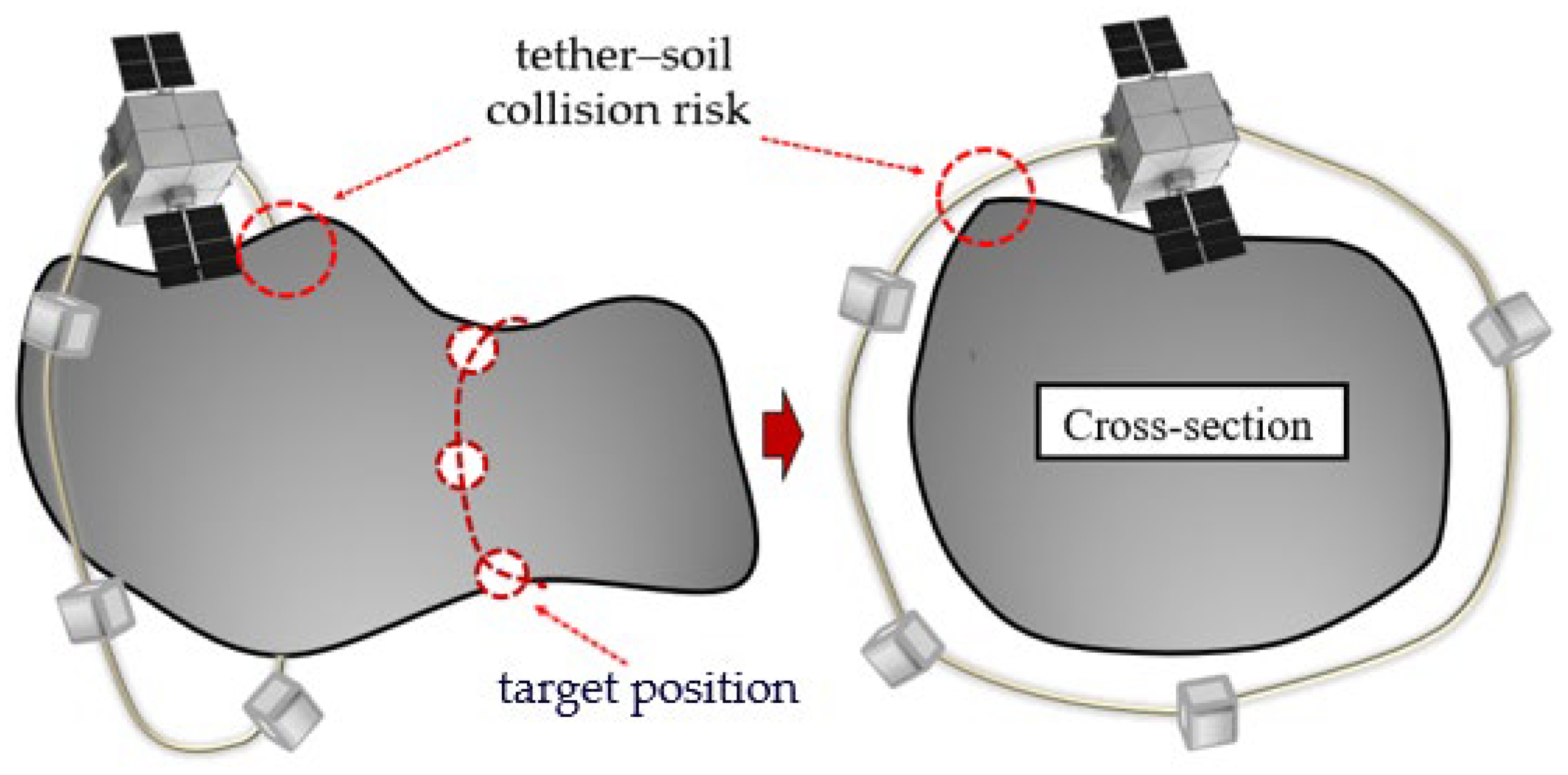
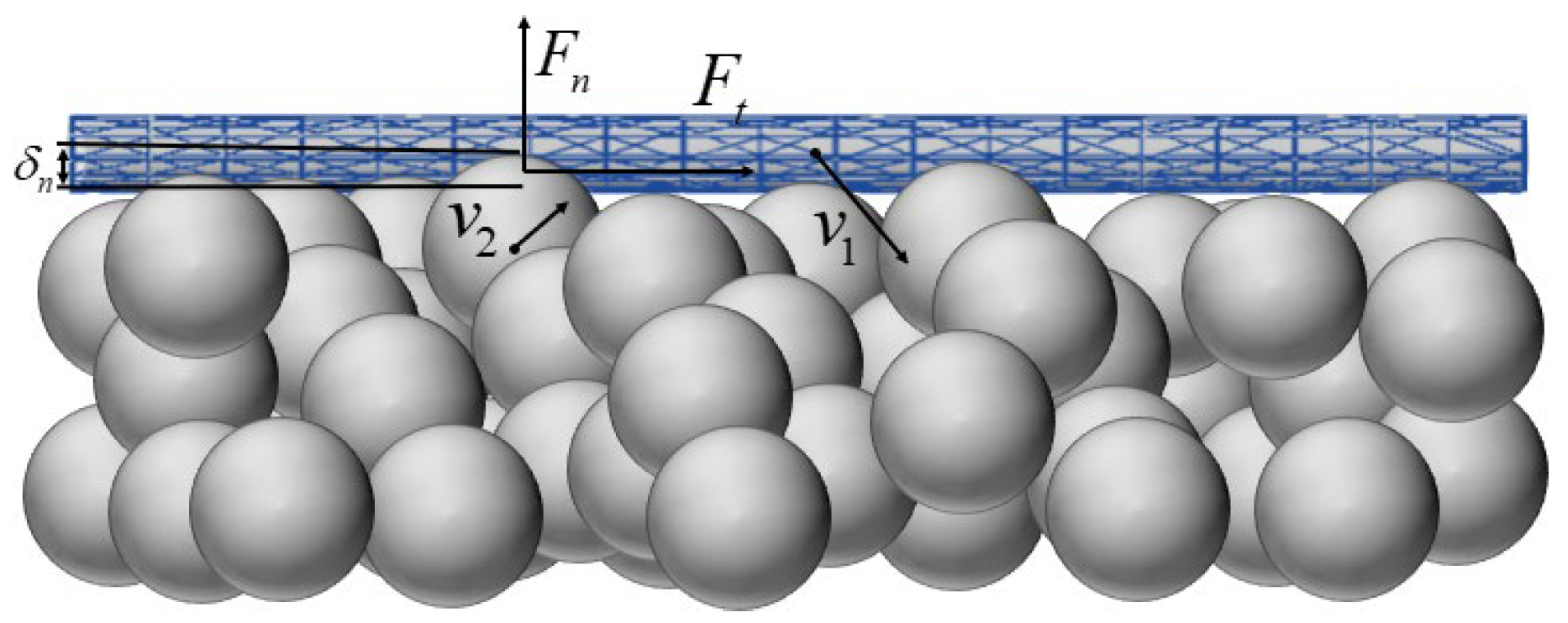
The above research only considers the interaction and reaction between the tether and the spacecraft. In addition to the tension force in the tethers within the system, the external forces considered are limited to gravity, and the influence of the tether–soil interaction on the position of the spacecraft is not considered. However, during the encirclement of small celestial bodies by multi-tethered spacecraft, the tether will collide with the asteroid soil, as shown in Figure 2. When the tether collides with the asteroid soil, an instantaneous impact force will be generated. This impact force will lead to a sharp increase in the tension of the tether and will also cause the dynamic response of the tether, such as vibration and fluctuation. When the tether collides with the asteroid soil, the impact force generated will be transmitted along the tether to the spacecraft connected to it. This force transmission may have a significant impact on the stability, attitude control, and overall structure of the spacecraft.

When the tether collides with the surface of a celestial body, the interaction generates an instantaneous impact force, leading to a dynamic alteration in the tension distribution within the tether. This energy transfer eventually acts on the connected spacecraft body. The instantaneous impact load will exert additional torque and acceleration on the spacecraft, perturb the original mechanical equilibrium state, and affect the displacement and attitude of the spacecraft. This not only requires the attitude control system to compensate for the attitude deviation in real time but also increases the prediction accuracy requirement of the control algorithm for the dynamic response.

In the field of research on low-velocity impacts on the asteroid soil of small celestial bodies, Reference [21] studied the Touch-And-Go Sample Acquisition Mechanism (TAGSAM) interaction with Bennu through numerical simulations using two collisional codes, PKDGRAV and GDC-I. Reference [22] utilized the Discrete Element Method (DEM) to simulate the general effects on the regolith of Phobos, thereby estimating the surface coefficient of restitution. Reference [23] applied the DEM simulation to test the formation of low-velocity craters (with velocities in the range of 5–50 cm/s) in granular materials under microgravity conditions. These studies have provided valuable insights and laid the groundwork for the establishment of the model in our current paper.

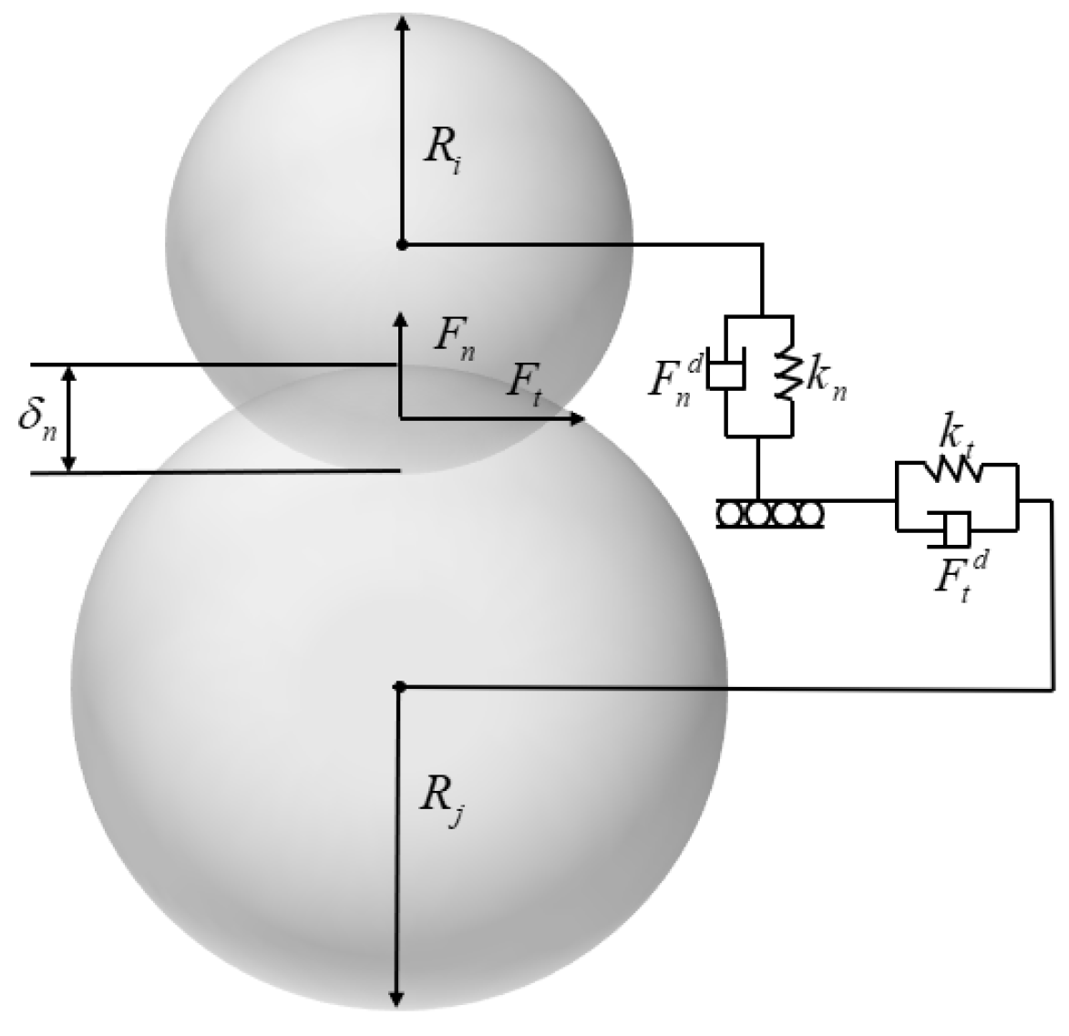
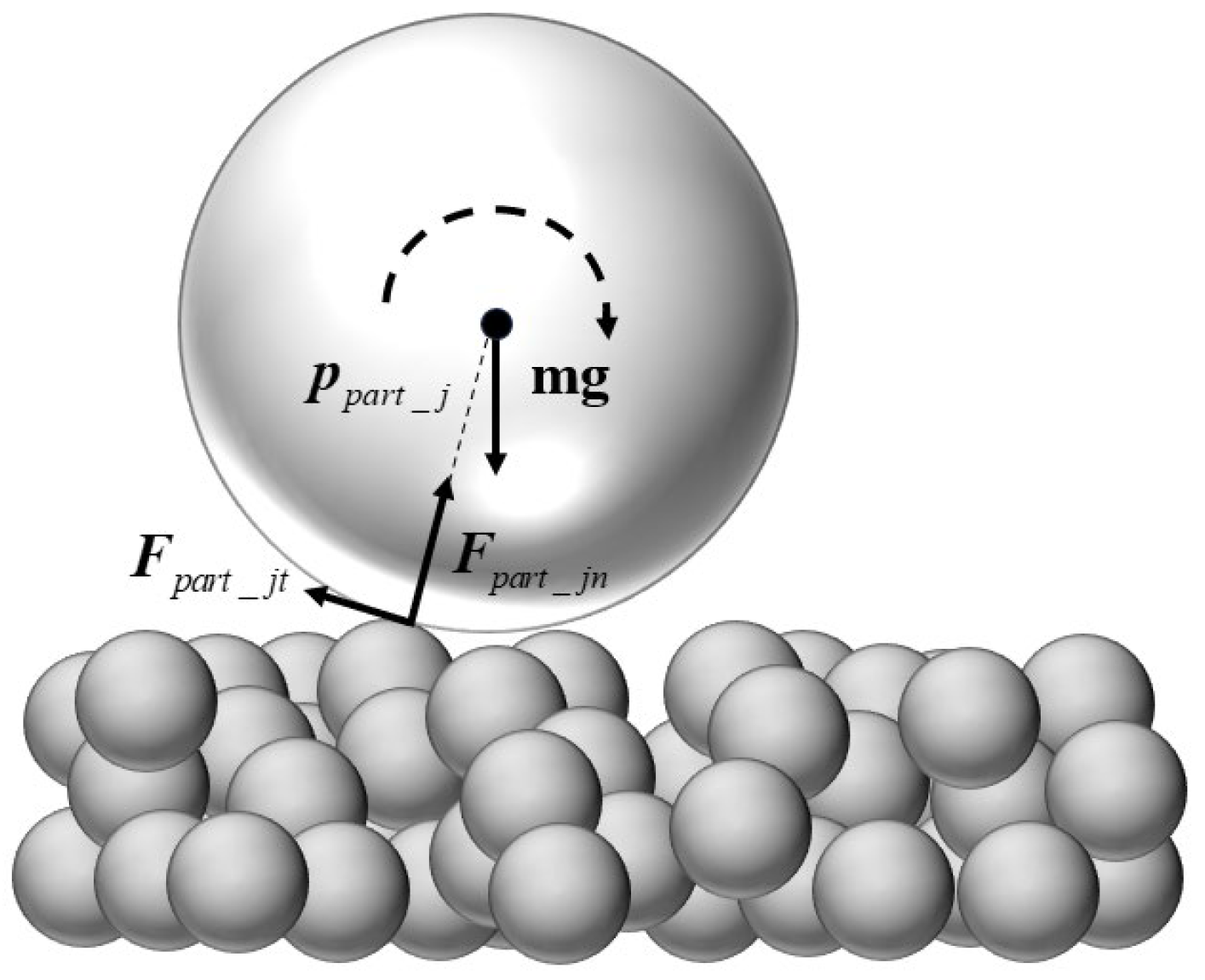
This paper proposes a coupling dynamic model based on a rigid–flexible coupling multi-body dynamics method and discrete element method to study the influence of tether–soil interaction on the trajectory of small celestial body detector. The multi-tethered spacecraft is simplified into a rigid–flexible coupling model of two satellites. The detector adopts a dual quaternion to establish a six-degree-of-freedom rigid body dynamics model. The tether adopts the chain rod model and combines the finite element method to model. The asteroid soil is modeled by the discrete element method. By comparing the displacement results of the detector in the tethered and untethered states, the influence of the tether–soil interaction on the trajectory of the small celestial detector is studied.

2. MTSF Dynamics Modeling

2.1. Contact Model with Gravel Layer

Small celestial bodies are modeled by the discrete element method, and the asteroid soil particles are simplified into spherical particles. The contact is calculated by the Hertz–Mindlin contact model [24,25,26].

Hertz–Mindlin contact model is mainly used for spherical particle contact, including the calculation of normal force, tangential force, and damping force. The contact force between the discrete elements can be divided into normal elastic force $F_n$, normal damping force $F_n^d$, tangential elastic force $F_t$, tangential damping force $F_t^d$, and rolling friction moment $T$. The Hertz–Mindlin contact model can be described by the spring–damper–slider model, as shown in Figure 3.

The Hertz theory [25] is used to calculate the normal elastic force. Based on the assumption of elastic half space, the nonlinear relationship between the normal contact force and the deformation is derived. The expression of the normal force $F_{\mathrm{n}}$ is as follows:

$$F_n={\displaystyle \frac{4}{3}}{E}^{\ast }{R}^{\ast {\displaystyle \frac{1}{2}}}{\delta }_n^{{\displaystyle \frac{3}{2}}}$$

(1)

Here, $E^{\ast }$ represents the equivalent elastic modulus between the two particles, $R^{\ast }$ represents the comprehensive curvature radius between the two particles, and ${\delta }_n$ represents the normal overlap of the two particles.

The comprehensive curvature radius $R^{\ast }$ is calculated by using the following formula:

$$R^{\ast }={\displaystyle \frac{R_1{R}_2}{R_1+R_2}}$$

(2)

Here, $R_1$ and $R_2$ represent the radius of the two particles, respectively.

The equivalent elastic modulus $E^{\ast }$ is calculated by using the following formula:

$$E^{\ast }={\displaystyle \frac{E_1{E}_2}{E_1(1-{\nu }_2^2)+E_2(1-{\nu }_1^2)}}$$

(3)

Here, $E_1$ and $E_2$ represent the elastic modulus of the two particles, respectively; $v_1$ and $v_2$ represent the Poisson ratio of the two particles, respectively.

Application of Mindlin–Deresiewicz theory [25]: According to the tangential displacement and stiffness of the contact area, the tangential force is calculated. The expression of tangential elastic force $F_t$ is as follows:

$$F_t=-S_t{\delta }_t$$

(4)

Here, $S_t$ represents tangential stiffness, and ${\delta }_t$ represents tangential overlap.

The tangential stiffness $S_t$ is calculated using the following formula:

$$S_{\mathrm{t}}=8G^{\ast }\sqrt{R^{\ast }{\delta }_t}$$

(5)

Here, $G^{\ast }$ represents the equivalent elastic shear modulus between two particles.

The equivalent elastic shear modulus $G^{\ast }$ is calculated using the following formula:

$$G^{\ast }={\displaystyle \frac{G_1{G}_2}{G_1(1-{\nu }_2)+G_2(1-{\nu }_1)}}$$

(6)

Here, $G_1$ and $G_2$ represent the elastic shear modulus of the two particles, respectively.

The damping model is used to calculate the damping force, and the energy dissipation is indirectly defined by the recovery coefficient to avoid direct measurement of the damping ratio of complex materials. The damping force is divided into tangential damping force and normal damping force.

The expression of normal damping force $F_n^d$ is as follows:

$$F_n^d=-2\sqrt{{\displaystyle \frac{5}{6}}}\beta \sqrt{S_n{m}^{\ast }}{v}_r^n$$

(7)

Here, $\beta$ represents the damping coefficient, $S_n$ represents the normal stiffness, $m^{\ast }$ represents the equivalent mass, and $v_r^n$ represents the normal relative velocity between the two particles.

The damping coefficient $\beta$ is calculated using the following formula:

$$\beta ={\displaystyle \frac{\ln e}{\sqrt{{\ln }^{2}e+{\pi }^2}}}$$

(8)

Here, $e$ represents the coefficient of restitution.

The normal stiffness $S_n$ is calculated using the following formula:

$$S_n=2E^{\ast }\sqrt{R^{\ast }{\delta }_n}$$

(9)

The equivalent mass $m^{\ast }$ is calculated using the following formula:

$$m^{\ast }={\displaystyle \frac{m_1{m}_2}{m_1+m_2}}$$

(10)

Here, $m_1$ and $m_2$ represent the mass of the two particles, respectively.

The expression of tangential damping force $F_t^d$ is as follows:

$$F_t^d=-2\sqrt{{\displaystyle \frac{5}{6}}}\beta \sqrt{S_t{m}^{\ast }}{v}_r^t$$

(11)

Here, $v_r^t$ represents the tangential relative velocity between the two particles.

Rolling friction is calculated by the independent torque model. The expression of rolling friction torque $T$ is as follows:

$$T=-{\mu }_r{F}_n{R}_i{\omega }_i$$

(12)

Here, ${\mu }_r$ represents rolling friction coefficient; $R_i$ represents the distance from the particle centroid to the contact point; and ${\omega }_i$ represents the unit angular velocity of the object at the contact point.

2.2. Small Celestial Body Detector Formation Dynamics

The small celestial body detector uses a dual quaternion [10,27] to establish a six-degree-of-freedom rigid body dynamics model. The dual quaternion combines quaternion and translation vectors to describe the rotation and translation of a rigid body and can deal with position and attitude at the same time.

The dual quaternion consists of a real part and dual part:

$$\widehat{\mathit{q}}={\mathit{q}}_r+\epsilon {\mathit{q}}_d$$

(13)

Here, $q_r,q_d\in {ℝ}^z$, where ${ℝ}^z$ represents the z-dimensional vector set; $q_r$ is a real part vector, describing rotation and representing rigid body attitude; $q_d$ is the dual part vector, describing translation and representing rigid body displacement; $\epsilon$ is the dual unit (satisfying ${\epsilon }^2=0,\epsilon \ne 0$); and the superscript $\widehat{·}$ represents the even number field.

The relative kinematic equation, that is, the derivative of the dual quaternion, is expressed as follows:

$${\dot{\widehat{q}}}_{A/B}={\displaystyle \frac{1}{2}}{\widehat{q}}_{A/B}\otimes {\widehat{\omega }}_{A/B}^A={\displaystyle \frac{1}{2}}{\widehat{\omega }}_{A/B}^B\otimes {\widehat{q}}_{A/B}$$

(14)

Here, the subscript $A,B$ represents the detector $A$ body coordinate system and the detector $B$ body coordinate system, and the superscript is the coordinate system expressed by the physical quantity; ${\widehat{q}}_{A/B}$ represents the six-degree-of-freedom transformation dual quaternion of the $A$ coordinate system relative to the $B$ coordinate system; ${\dot{\widehat{q}}}_{A/B}$ is its derivative with respect to time; and ${\widehat{\omega }}_{A/B}^A$ represents the velocity spinor of the $A$ coordinate system relative to the $B$ coordinate system.

The rigid body dynamics equation is expressed as follows:

$${\dot{\widehat{\mathit{\omega }}}}_{A/I}^A=-{\widehat{\mathit{\omega }}}_{A/I}^A\times {\widehat{\mathit{J}}}_A{\widehat{\mathit{\omega }}}_{A/I}+{\widehat{\mathit{F}}}_A^A$$

(15)

Here, the subscript $I$ represents the inertial system; ${\widehat{J}}_A$ represents the dual inertia matrix of the detector $A$; ${\widehat{F}}_A^A$ represents the dual external force acting on the detector $A$, the dual external force acting on the $A$ coordinate system, where ${\widehat{F}}_A^A=F_A^A+\epsilon M_A^A$, and the dual external force and the couple external torque acting on the center of mass of the detector $A$, respectively. ${\widehat{\mathit{\omega }}}_{A/I}^A$ and ${\dot{\widehat{\omega }}}_{A/I}^A$, respectively, are the velocity spinor of the $A$ coordinate system relative to the $I$ coordinate system and the expression in the $A$ coordinate system’s time derivative.

The relative dynamic model of the $i$-node spacecraft relative to the centroid of the small celestial body is

$$\begin{array}{c}{\widehat{J}}_i{\dot{\widehat{\omega }}}_{i/B}^i=-{\widehat{\omega }}_{i/I}^i\times {\widehat{J}}_i{\widehat{\omega }}_{i/I}^i-{\widehat{J}}_i({\widehat{q}}_{i/B}^{\ast }\otimes {\dot{\widehat{\omega }}}_{B/I}^B\otimes {\widehat{q}}_{i/B})\\ +{\widehat{J}}_i\left({\widehat{\omega }}_{i/B}^i\times ({\widehat{q}}_{i/B}^{\ast }\otimes {\widehat{\omega }}_{B/I}^B\otimes {\widehat{q}}_{i/B})\right)+{\widehat{F}}_i^i\end{array}$$

(16)

In the external force term, in addition to the irregular dual gravity of the small celestial body, the dual tether force, the dual control force, etc., the force and moment of the granular medium on the node spacecraft should also be included. Therefore, the coupled external force can be expressed as

$${\widehat{\mathit{F}}}_i^i={\widehat{\mathit{F}}}_s^i+{\widehat{\mathit{F}}}_a^i+{\widehat{\mathit{F}}}_u+{\displaystyle \sum }_{k=1}^n{\widehat{\mathit{a}}}_{ik}\odot {\widehat{\mathit{F}}}_{Tk}^i+{\displaystyle \sum }_{j=1}^m{\widehat{\mathit{\beta }}}_j\odot {\widehat{\mathit{F}}}_{part\_j}^i$$

(17)

Here, ${\widehat{F}}_u=F_u+\epsilon {\tau }_u$ represents the dual control force; $F_u$ and ${\tau }_u$ are the control force and control torque of the node spacecraft actuator, respectively; ${\widehat{F}}_a=F_a+\epsilon {\tau }_a$ represents the dual gravity of a small celestial body; $F_a$ and ${\tau }_a$ are the gravity of a small celestial body and the gravitational gradient moment, respectively; ${\widehat{F}}_s$ represents the gravity of other related celestial bodies; ${\widehat{F}}_{Tk}=F_{ik}^{Tw}+\epsilon F_{ik}^{Tw}\times L_{wik}$ is the dual tether force; ${\displaystyle {\displaystyle \sum }_{j=1}^m}{\widehat{\mathit{\beta }}}_j\odot {\widehat{\mathit{F}}}_{part\_j}^i$ is the dual collision force of a total of $m$ particles received by the node-based spacecraft; and ${\widehat{\mathit{F}}}_{part\_j}^i$ is the dual collision force of the $j$ particle medium to the node-based spacecraft, as shown in Figure 4.

The expression of ${\widehat{F}}_{part\_j}^i$ is

$${\widehat{\mathit{F}}}_{part\_j}^i={\mathit{F}}_{part\_jn}+\epsilon {\mathit{F}}_{part\_jt}\times {\mathit{p}}_{part\_jt}$$

(18)

Here, ${\mathit{p}}_{part\_jt}$ is the displacement of the contact position between the particle medium and the node-based spacecraft from the center of mass of the node-based spacecraft. ${\mathit{F}}_{part\_jn}$ and ${\mathit{F}}_{part\_jt}$ are the normal and tangential forces of the contact impact force on the force axis, respectively, and include the damping force and elastic force. The calculation method is the same as the inter-particle force in the upper summary, and it is no longer repeated.

2.3. Flexible Tether Dynamics

The tether is established by combining the chain rod model and the finite element method. The core idea of modeling is to divide the continuous tether structure into discrete elements and simulate the mechanical behavior of the tether by setting physical properties and boundary conditions.

The chain rod model [28] is used to discretize the tether into a series of rigid straight rods connected by spherical motion pairs, which can fully consider the flexibility of the tether. The finite element method further divides each rigid segment into finite element mesh and converts it into a flexible body. The finite element method can fully consider the elasticity of the tether. The tether model is shown as Figure 5.

The motion equation of the flexible body chain rod model is expressed by the Lagrange equation, and the expression is as follows:

$${\displaystyle \frac{\mathrm{d}}{\mathrm{d}t}}\left({\displaystyle \frac{\partial T}{\partial {\dot{q}}_i}}\right)-{\displaystyle \frac{\partial T}{\partial q_i}}+{\displaystyle \frac{\partial U}{\partial q_i}}=F_i$$

(19)

Here, $T$ represents the kinetic energy of the system, $U$ represents the potential energy of the system, $q_i$ represents the generalized coordinates describing the degree of freedom of the system, and $F_i$ represents the non-conservative force corresponding to the generalized coordinates.

The continuous Lagrange equation is transformed into the form of discrete linear equations. The expression is as follows:

$$M_{ab}{\ddot{u}}^b+C_{ab}{\dot{u}}^b+K_{ab}{u}^b=F_{ab}$$

(20)

Here, $M_{ab}$ is the mass matrix, describing the inertial characteristics of the system; $C_{ab}$ is the damping matrix, describing the damping characteristics of the system; $K_{ab}$ is the stiffness matrix, describing the elastic restoring force of the system; $F_{ab}$ is the external force vector, which is composed of the body force, surface force, and concentrated force; and $u^b$, ${\dot{u}}^b$, and ${\ddot{u}}^b$ are the node displacement, velocity, and acceleration vectors, respectively.

The calculation of the contact force between the tether elastomer model and the asteroid soil discrete element model is shown in Figure 6.

Considering that only the elements adjacent to the element have short-range force in the discrete element calculation, and combined with the calculation characteristics of the finite element that can deal with continuous media, long-range forces, and complex boundary conditions, the calculation model with a layer of transition layer [29] is adopted as shown in Figure 7. In the transition layer, the finite element is treated as a discrete element with an infinite radius. The contact force method between the discrete element and the finite element in the transition layer is the same as the contact calculation method between the particles in Section 1, and the Hertz–Mindlin model is used. The discrete element and finite element in the transition boundary provide boundary conditions for each other, and the discrete element region and the finite element region outside the transition layer are solved according to their respective methods.

The selection of time step needs to consider the stability requirements of both discrete element method and finite element method.

The discrete element solution step size requires that the discrete elements cannot penetrate each other in one step, that is

$$F_{ij}\Delta t=m_j{v}_j\le M$$

(21)

Here, $F_{ij}\Delta t$ is the impulse, $m_j{v}_j$ is the momentum obtained by the particles $j$, and $M$ is the maximum momentum that the particles $j$ can obtain during the entire collision process.

The stability condition of the finite element solution step size is as follows:

$$\Delta t\le T_n/\pi$$

(22)

Here, $T_n$ is the minimum natural vibration period of the finite element system.

Usually, the time step taken by the discrete element is a few hundredths of the critical step, which is significantly smaller than the finite element. For simplicity, the same time step is used in the combination method, that is, the time step determined by the discrete element [29].

3. Numerical Simulation

3.1. Initial Condition

In this paper, the rigid–flexible coupling multi-body dynamics modeling method and the discrete element method are used to establish the spacecraft–tether dynamics model and the asteroid soil dynamics model. The two models are coupled to form the spacecraft–tether system–particle medium collision dynamics model. The displacement results of the detector in two states of tethered and untethered at different collision speeds are compared to explore the influence of the tether–soil interaction on the trajectory of the small celestial body detector.

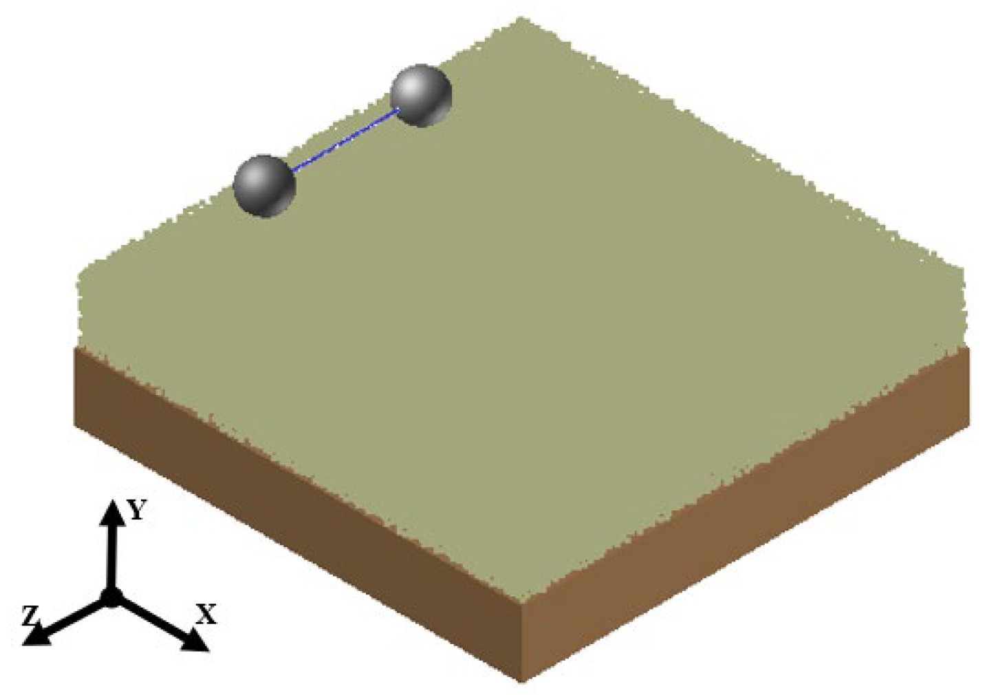
The spacecraft rigid body model, the tether chain rod model, and the small body surface particle discrete element model are combined to form a coupling simulation model. The coordinate axis is defined as Figure 8, the X direction is the forward direction of the detector, the Y direction is the downward direction of the detector, and the Z direction is the axial direction of the tether. The weak gravitational acceleration of the small body is selected as 0.01 m/s², and the direction is the negative direction of the Y-axis.

The spacecraft is simplified as a homogeneous spherical rigid body, and the specific parameters are as follows. The quality of the spacecraft is 10 kg. In terms of moments of inertia, $I_{xx}$, $I_{yy}$, and $I_{zz}$ all have a numerical value of 0.04 kg·m². Additionally, the radius of the spacecraft is 0.1 m.

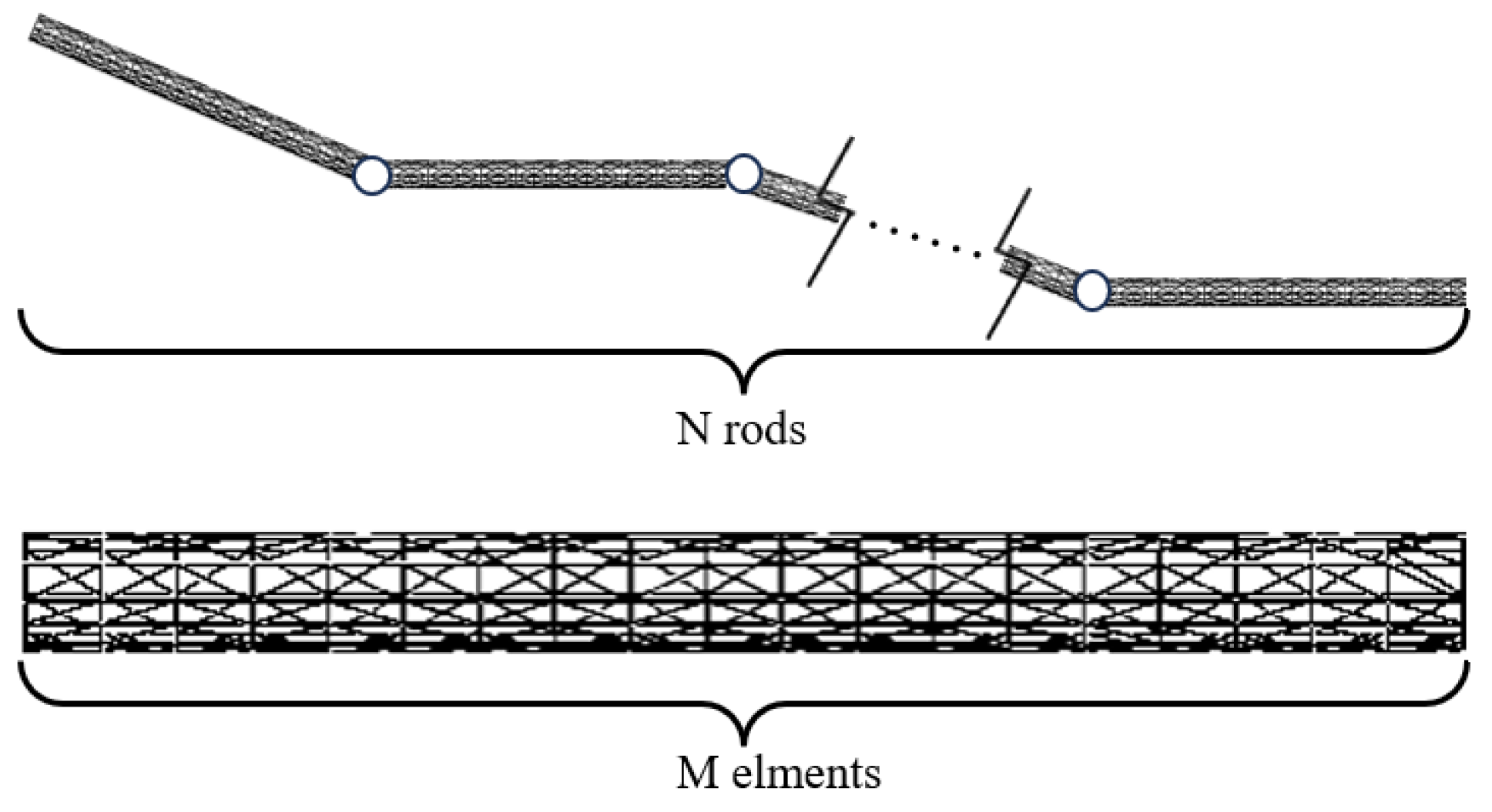
The tether is composed of 10 flexible rods with a length of 50 mm connected by a ball hinge, with a total length of 500 mm. Regarding the material parameters of the tether, the elastic modulus is 200 GPa, the density is 7850 kg/m³, Poisson’s ratio is 0.285, and the damping coefficient is 0.0001.

The gravel layer particles are simplified as spherical particles, and the relevant characteristic parameters [14] are as follows: the particle diameter is 20 mm, the density of the granular material is 2790 kg/m³, the particle Poisson ratio is 0.3, the restitution coefficient is 0.8, the rolling friction coefficient is 0.1, and the static friction coefficient is 1.5. In addition, the particle depth is 300 mm, the gravel roughness height is 300 mm, and the gravel groove side length is 2 m.

In terms of contact characteristic parameters, the contact characteristic parameters between particles and the tether (P–T) and between particles and the detector (P–D) are as follows, respectively: the restitution coefficient between the particles and the tether is 0.8, the rolling friction coefficient is 0.25, and the static friction coefficient is 1.2; the restitution coefficient between the particles and the detector is 0.8, the rolling friction coefficient is 0.25, and the static friction coefficient is 1.2.

3.2. Operating Conditions Setting

To comparing the tethered and untethered conditions, this paper sets up three groups of comparative simulations with different speeds based on the above model. There are six operating conditions (OC) under different speeds, including untethered and tethered conditions, as shown in

Table 1. Operating conditions setting.

OC	Untethered/Tethered	Vy (mm/s)	Vx (mm/s)
1	Untethered	−100	−300
2	Tethered	−100	−300
3	Untethered	−100	−200
4	Tethered	−100	−200
5	Untethered	−100	−100
6	Tethered	−100	−100

Operating condition 1 and 2 form Comparison 1, operating condition 3 and 4 form Comparison 2, and operating condition 5 and 6 form Comparison 3.

.

3.3. Simulation Result

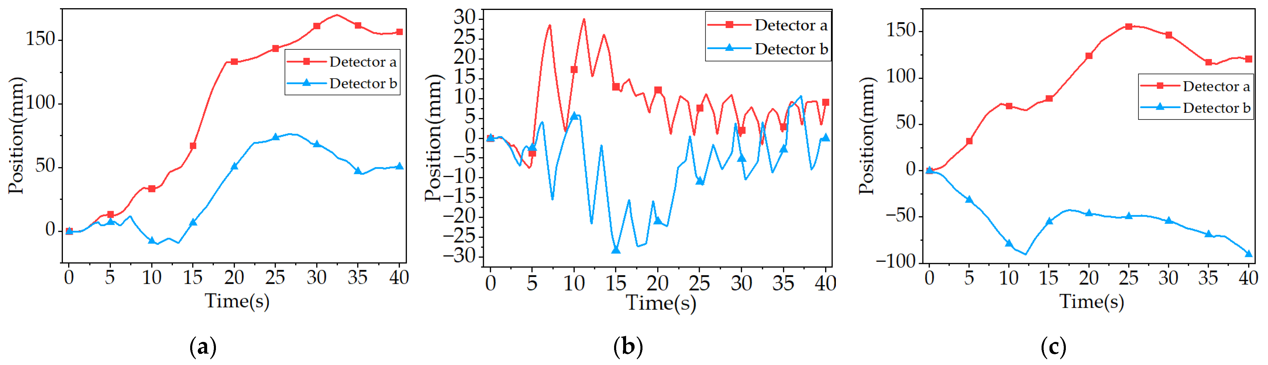
Because there are two operating conditions in each group of comparisons, and there are two detectors in each operating condition, in order to facilitate the comparison, in the result diagram, the untethered system is indicated by the dotted line, the tethered system is indicated by the real line, Detector a is indicated by the symbol ‘$\square$’, and Detector b is indicated by the symbol ‘$△$’.

3.3.1. Comparison 1

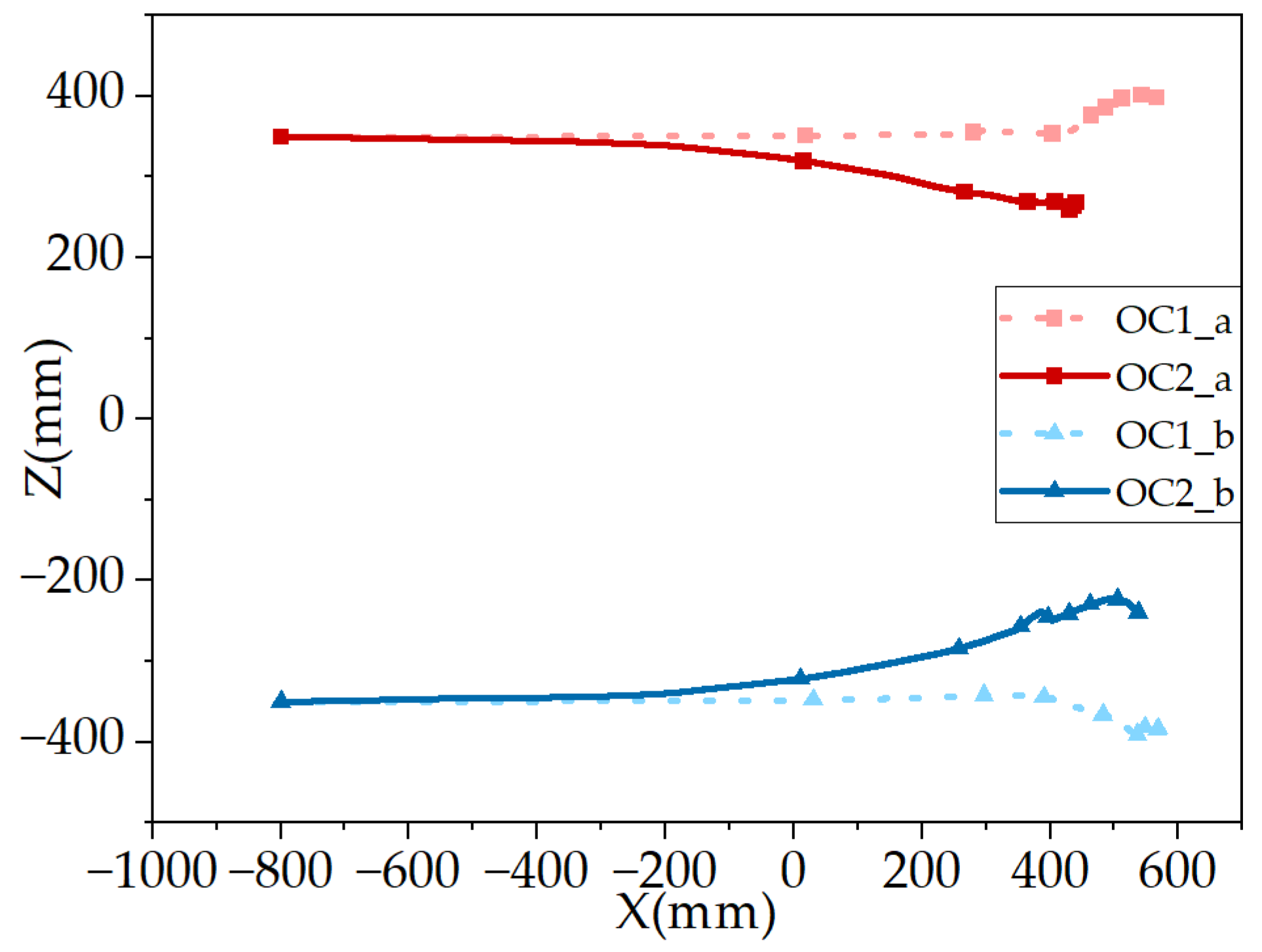
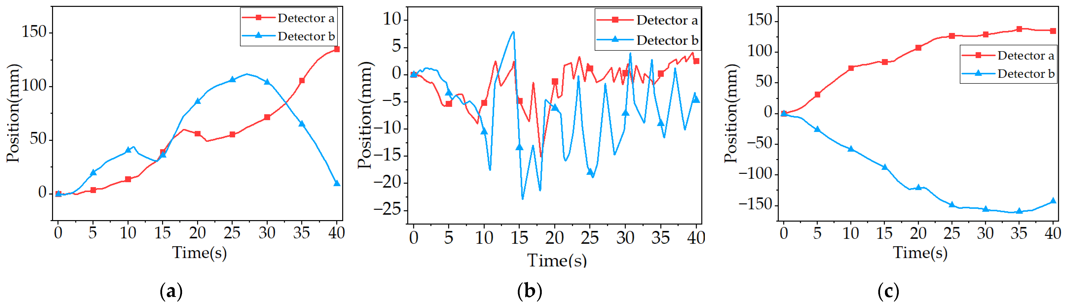
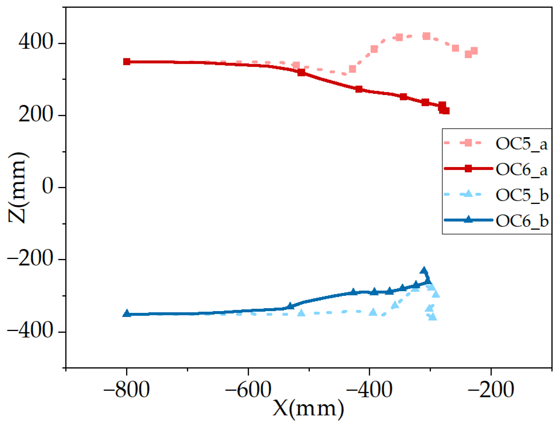
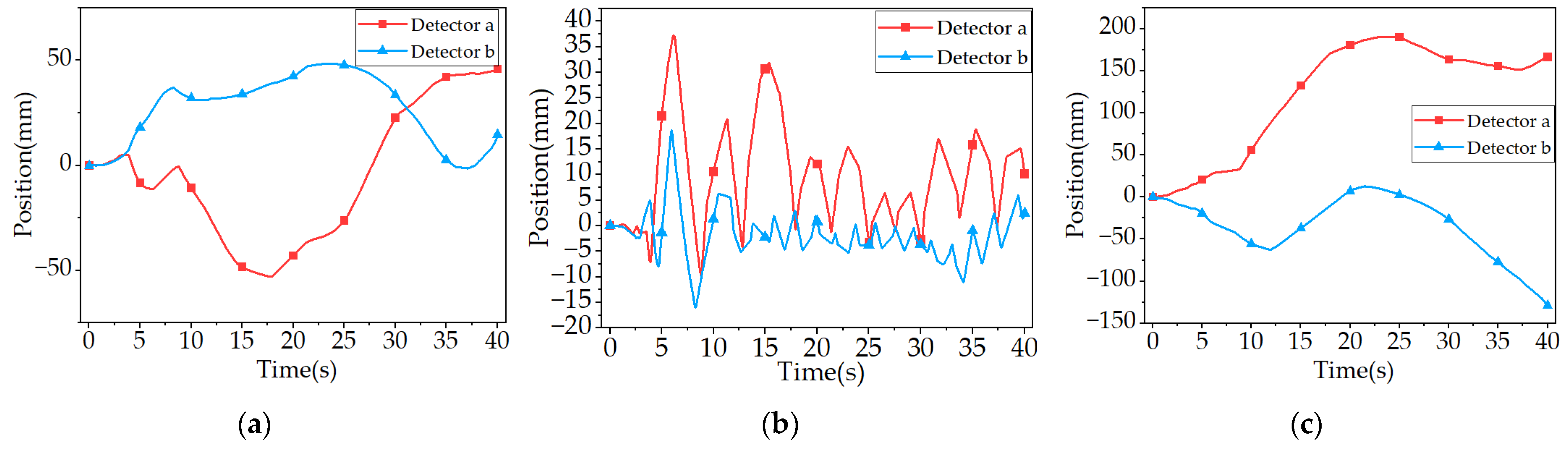
The top view of the detector trajectory in conditions 1 and 2 is shown in Figure 9, and the time interval between each symbol is 5 s.

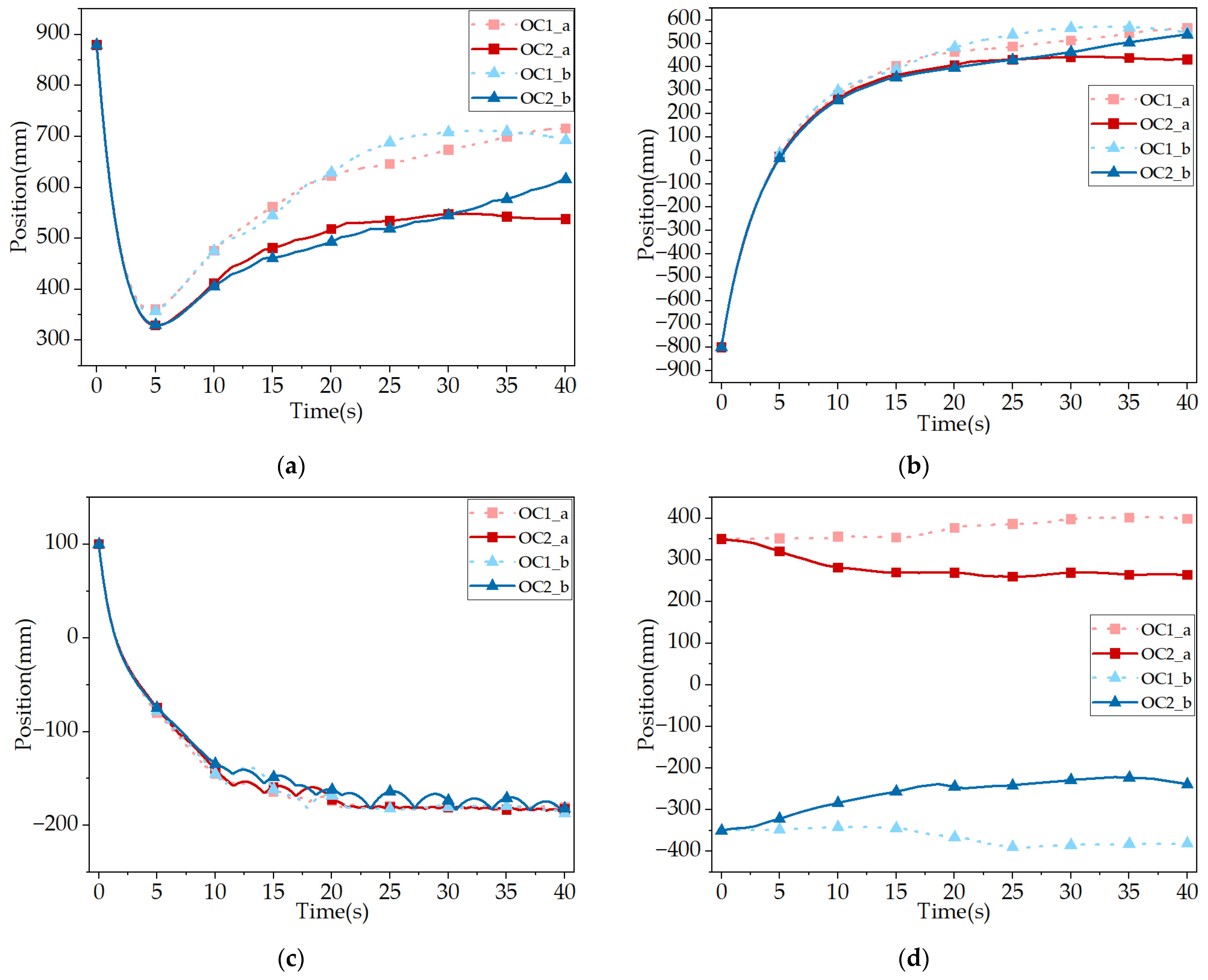
The displacement results of operating conditions 1 and 2 are shown in Figure 10.

According to Figure 10, under the condition of an X-direction speed of 300 mm/s and a Y-direction speed of −100 mm/s, the forward displacement of the detector in the tethered system is generally lower than that of the detector in the untethered system. The time required for the detector to drop to the same position in the tethered system is longer than that in the untethered system; compared with the detector in the untethered system, the detector in the tethered system has obvious displacement in the axial direction of the tether, and the detector moves closer to the other detector.

The results of the displacement difference between the detectors corresponding to operating conditions 1 and 2 are shown in Figure 11.

From the analysis of the above figure, the maximum displacement deviation in the X-direction can reach 135.0 mm, the maximum displacement deviation in the Y-direction can reach 22.9 mm, and the maximum displacement deviation in the Z-direction can reach 161.0 mm.

In the X-direction, the final displacement difference in Detector a in the untethered and tethered states accounts for 9.9% of its total displacement in the untethered state; the final displacement difference in Detector b in the untethered and tethered states accounts for 0.7% of its total displacement in the untethered state. In the Z-direction, the displacement difference between the beginning and end of Detector a in the tethered system is 1.78 times that in the untethered system. The displacement difference between the beginning and end of Detector b in the tethered system is 3.52 times that in the untethered system.

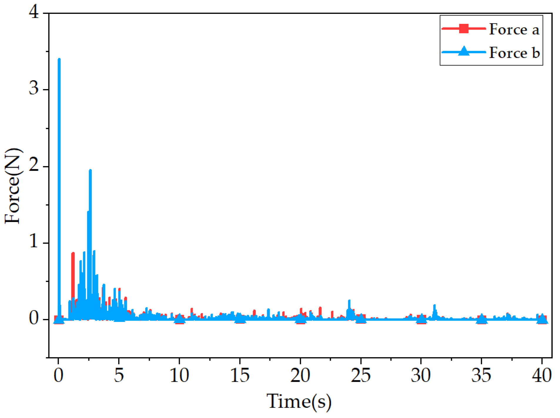
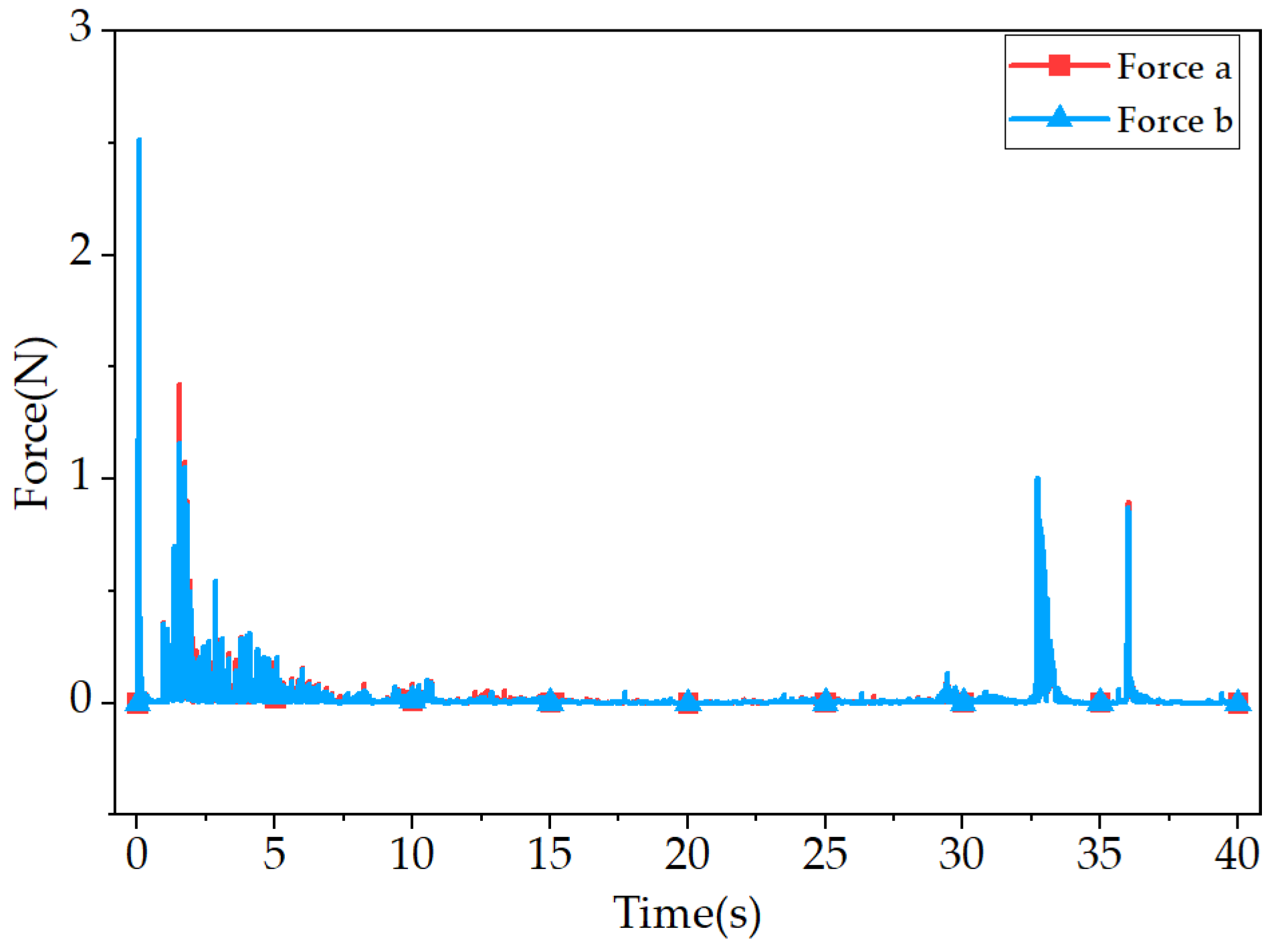
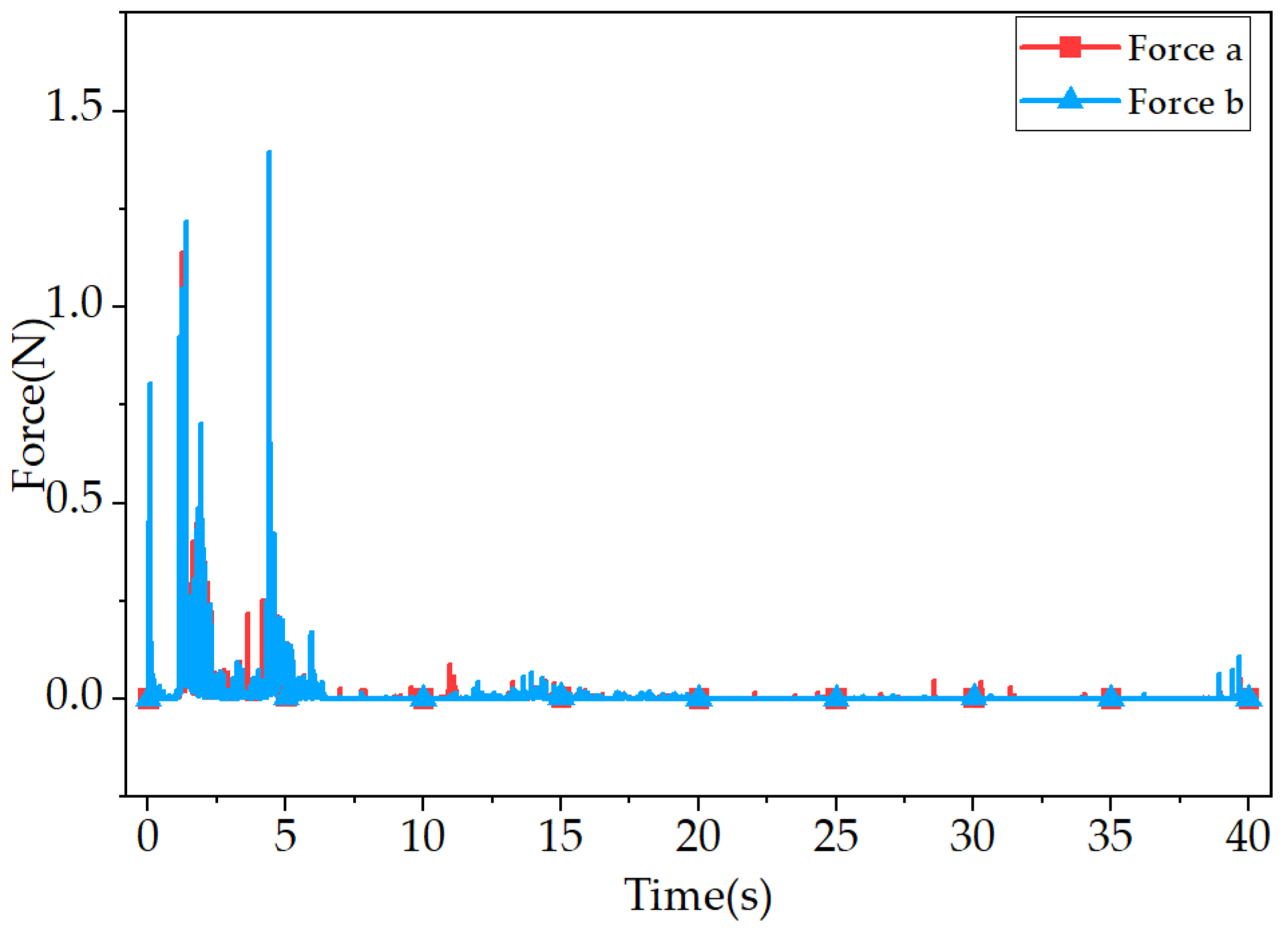
The force at the tether–detector connection in operating condition 2 is shown in Figure 12. The force transmitted by the tether–soil interaction to the detector can reach a maximum of 3.41 N.

3.3.2. Comparison 2

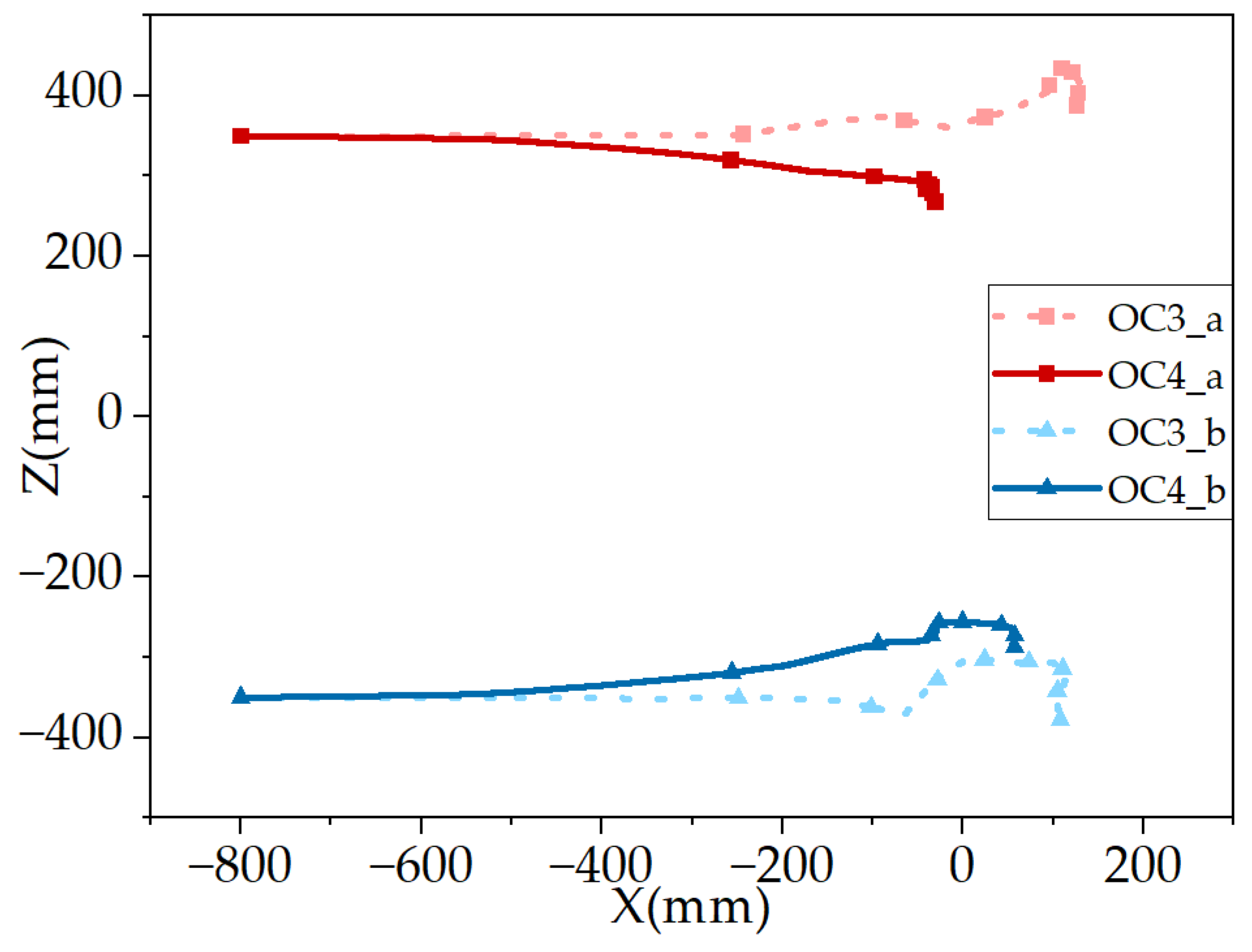
The top view of the detector trajectory in conditions 3 and 4 is shown in Figure 13, and the time interval between each symbol is 5 s.

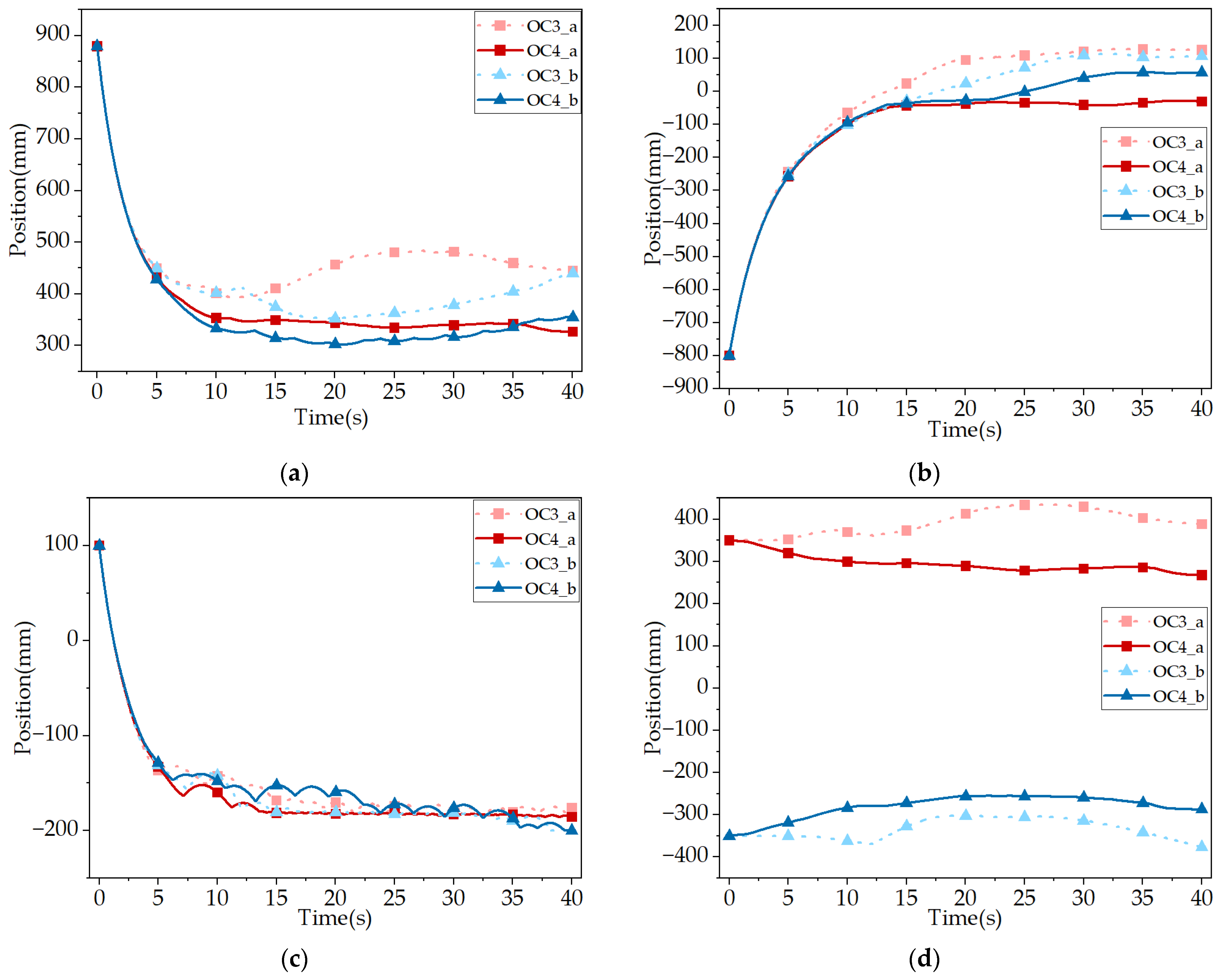
The displacement results of operating conditions 3 and 4 are shown in Figure 14.

According to the figure, under conditions of an X-direction speed of 200 mm/s and a Y-direction speed of −100 mm/s, the displacement law of the detector is the same as that in Comparison 1, and it will not be described here.

The results of the displacement difference between the detectors corresponding to operating conditions 3 and 4 are shown in Figure 15.

From the analysis of the above figure, the maximum displacement deviation in the X-direction can reach 170.2 mm, the maximum displacement deviation in the Y-direction can reach 30.1 mm, and the maximum displacement deviation in the Z-direction can reach 156.3 mm.

In the X-direction, the final displacement difference in Detector a in the untethered and tethered states accounts for 16.9% of its total displacement in the untethered state; the final displacement difference in Detector b in the untethered and tethered states accounts for 5.6% of its total displacement in the untethered state. In the Z-direction, the displacement difference between the beginning and end of Detector a in the tethered system is 2.15 times that in the untethered system. The displacement difference between the beginning and end of Detector b in the tethered system is 2.32 times that in the untethered system.

The force at the tether–detector connection in operating condition 4 is shown in Figure 16. The force transmitted by the tether–soil interaction to the detector can reach a maximum of 2.52 N.

3.3.3. Comparison 3

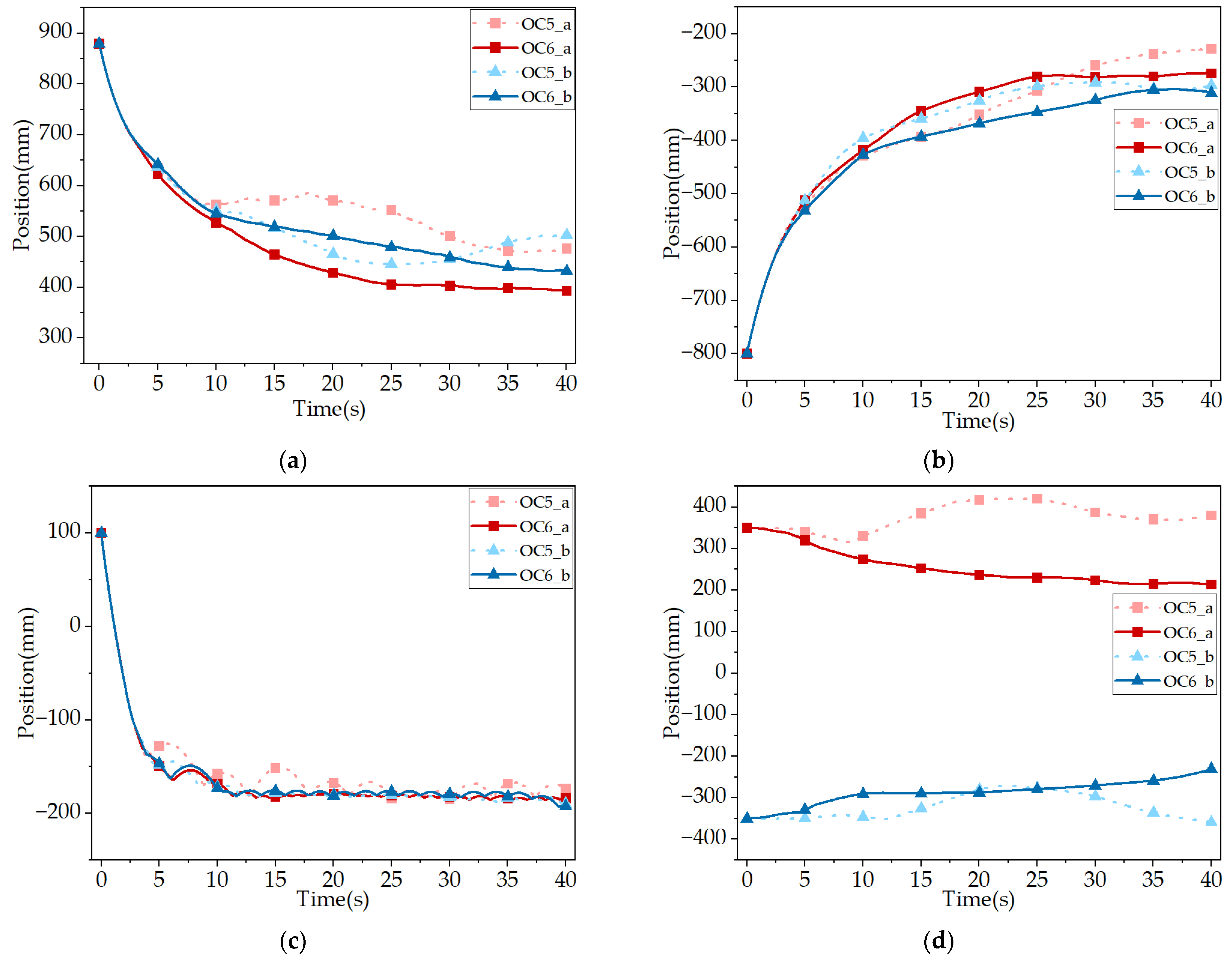
The top view of the detector trajectory in conditions 5 and 6 is shown in Figure 17, and the time interval between each symbol is 5 s.

The displacement results of operating conditions 5 and 6 are shown in Figure 18.

According to the figure, under conditions of an X-direction speed of 100 mm/s and a Y-direction speed of −100 mm/s, the displacement law of the detector is the same as that in Comparison 1, and it will not be described here.

The results of the displacement difference between the detectors corresponding to operating conditions 5 and 6 are shown in Figure 19.

From the analysis of the above figure, the maximum displacement deviation in the X-direction can reach 53.0 mm, the maximum displacement deviation in the Y-direction can reach 37.3 mm, and the maximum displacement deviation in the Z-direction can reach 190.6 mm.

In the X-direction, the final displacement difference in Detector a in the untethered and tethered states accounts for 8.0% of its total displacement in the untethered state; the final displacement difference in Detector b in the untethered and tethered states accounts for 2.9% of its total displacement in the untethered state. In the Z-direction, the displacement difference between the beginning and end of Detector a in the tethered system is 4.59 times that in the untethered system. The displacement difference between the beginning and end of Detector b in the tethered system is 13.16 times that in the untethered system.

The force at the tether–detector connection in operating condition 6 is shown in Figure 20. The force transmitted by the tether–soil interaction to the detector can reach a maximum of 1.39 N.

4. Discussion

In this paper, based on the multi-body dynamics method and the discrete element method, the spacecraft–tether–soil coupling dynamics model is established for the risk of tether–soil collision that may exist in the process of multi-tethered spacecraft encircling and capturing small celestial bodies. According to the simulation results, the influence of tether–soil interaction on the trajectory of the detector is analyzed, and the following conclusions are obtained:

The influence of tether–soil interaction on the trajectory of the detector is mainly reflected in the displacement of the detector along the axial direction of the tether. In the forward direction of the detector, the tether–soil interaction reduces the forward displacement of the detector. In the axial direction of the tether, the tether–soil interaction makes the two detectors move closer to each other, and the displacement changes greatly.

In view of the constraints of time and the current authors’ competences, this topic can be further promoted in the following directions in a follow-up study:

• Integrating the control system: Spacecraft adaptive control and tether retraction control are integrated into the coupled dynamics model to study the attitude stability, orbit maintenance, and other control problems of the spacecraft in a complex environment, so as to improve the autonomous decision-making and execution ability of the spacecraft. Aiming at the dynamic characteristics of the tether during the retraction process, key technologies, such as tension control and speed adjustment of the tether, are studied to ensure the stability and safety of the tether during the retraction process.
• The relationship between tether dynamics and displacement differences in granular material deserves further attention. A comprehensive analysis of tether–particle interactions could significantly enhance our understanding of the physical processes at play. Thus, we propose this as a critical future research direction, with the potential to unlock new insights into the behavior of systems involving granular materials and tether-like structures.

References

1. Wang, T.; Quan, Q.; Tang, D.; Deng, Z. Progress in the development of small-celestial-body anchoring robots. Nat. Astron. 2023, 7, 380–390. [Google Scholar] [CrossRef]
2. Cui, P.Y.; Yuan, X.; Zhu, S.Y.; Qiao, D. Research progress of small body autonomous landing techniques. Yuhang Xuebao/J. Astronaut. 2016, 37, 759–767. [Google Scholar]
3. Gong, Z.; Li, M.; Chen, C.; Zhao, C. The frontier science and key technologies of asteroid monitoring and early warning, security defense and resource utilization. Chin. Sci. Bull. 2020, 65, 346–372. [Google Scholar] [CrossRef]
4. Cheng, B.; Yu, Y.; Baoyin, H. Recent advances in granular dynamics for small-body touchdown missions. Sci. Sin. Technol. 2021, 51, 1299–1314. [Google Scholar] [CrossRef]
5. Yano, H.; Kubota, T.; Miyamoto, H.; Okada, T.; Scheeres, D.; Takagi, Y.; Yoshida, K.; Abe, M.; Abe, S.; Barnouin, O.; et al. Touchdown of the hayabusa spacecraft at the muses sea on itokawa. Science 2006, 312, 1350–1353. [Google Scholar] [CrossRef]
6. Zhang, X.; Zhang, G.Q.; Xie, H.P.; Gao, M.Z.; Wen, Y.F. A review of sampling exploration and devices for extraterrestrial celestial bodies. Space Sci. Rev. 2022, 218, 59. [Google Scholar] [CrossRef]
7. Wei, Z.; Qinkun, C.; Junlin, L. Technical progress in the utilization and exploitation of small celestial body resources. Acta Astronaut. 2023, 208, 219–255. [Google Scholar]
8. Feng, J.; Hou, X.; Armellin, R. Survey on studies about model uncertainties in small body explorations. Prog. Aeosp. Sci. 2019, 110, 100549. [Google Scholar] [CrossRef]
9. Morgan, P.; Grott, M.; Knapmeyer-Endrun, B.; Golombek, M.; Delage, P.; Lognonné, P.; Piqueux, S.; Daubar, I.; Murdoch, N.; Charalambous, C.; et al. A pre-landing assessment of regolith properties at the InSight landing site. Space Sci. Rev. 2018, 214, 104. [Google Scholar] [CrossRef]
10. Yang, Y.; Huang, Y.; Zhang, H.; Tian, H.; Zhao, Y. A method for capturing small body in close proximity multi-body tethered spacecraft formations. Sci. Sin. Phys. Mech. Astron. 2024, 54, 234511. [Google Scholar] [CrossRef]
11. Yang, Y.; Huang, Y.; Tian, H.; Zhu, Y.; Qian, C.; Zhao, Y. Design and experimental verification of multi-tethered spacecraft formation encircled to capture small celestial body system. Acta Astronaut. 2025, 229, 65–76. [Google Scholar] [CrossRef]
12. Liu, J.; Li, G.; Zhu, Z.H.; Zhan, X. Orbital boost characteristics of spacecraft by electrodynamic tethers with consideration of electric-magnetic-dynamic energy coupling. Acta Astronaut. 2020, 171, 196–207. [Google Scholar] [CrossRef]
13. Liu, J.; Zhu, Z.H.; Li, G.; Zhan, X. Fuzzy-based continuous current control of electrodynamic tethers for stable and efficient orbital boost. Aerosp. Sci. Technol. 2021, 118, 106999. [Google Scholar] [CrossRef]
14. Yang, Y.; Tian, H.; Shi, J.; Ge, D.; Xu, J.; Huang, Y. Design and stability analysis of attachment buffer system for small celestial body detector. J. Deep. Space Explor. 2024, 11, 559–569. [Google Scholar]
15. Kim, M.; Hall, C. Dynamics and control of tethered satellite systems for NASA’s SPECS mission. Adv. Astronaut. Sci. 2003, 116, 1–20. [Google Scholar]
16. Nakaya, K.; Iai, M.; Omagari, K.; Yabe, H.; Matunaga, S. Formation deployment control for spinning tethered formation flying—Simulations and ground experiments. In Proceedings of the AIAA Guidance, Navigation, and Control Conference and Exhibit, Providence, RI, USA, 16–19 August 2004. [Google Scholar]
17. Sun, L.; Zhao, G.; Huang, H. Stability and control of tethered satellite with chemical propulsion in orbital plane. Nonlinear Dyn. 2013, 74, 1113–1131. [Google Scholar] [CrossRef]
18. Lim, J.; Chung, J. Dynamic analysis of a tethered satellite system for space debris capture. Nonlinear Dyn. 2018, 94, 2391–2408. [Google Scholar] [CrossRef]
19. Luo, C.Q.; Sun, J.L.; Wen, H.; Jin, D.P. Dynamics of a tethered satellite formation for space exploration modeled via ANCF. Acta Astronaut. 2020, 177, 882–890. [Google Scholar] [CrossRef]
20. Cai, Z.; Li, X.; Zhou, H. Nonlinear dynamics of a rotating triangular tethered satellite formation near libration points. Aerosp. Sci. Technol. 2015, 42, 384–391. [Google Scholar] [CrossRef]
21. Ballouz, R.; Walsh, K.J.; Sánchez, P.; Holsapple, K.A.; Michel, P.; Scheeres, D.J.; Zhang, Y.; Richardson, D.C.; Barnouin, O.S.; Nolan, M.C.; et al. Modified granular impact force laws for the OSIRIS-REx touchdown on the surface of asteroid (101955) bennu. Mon. Not. Roy. Astron. Soc. 2021, 507, 5087–5105. [Google Scholar] [CrossRef]
22. Çelik, O.; Baresi, N.; Ballouz, R.; Ogawa, K.; Wada, K.; Kawakatsu, Y. Ballistic deployment from quasi-satellite orbits around phobos under realistic dynamical and surface environment constraints. Planet Space Sci. 2019, 178, 104693. [Google Scholar] [CrossRef]
23. Çelik, O.; Ballouz, R.; Scheeres, D.J.; Kawakatsu, Y. A numerical simulation approach to the crater-scaling relationships in low-speed impacts under microgravity. Icarus 2022, 377, 114882. [Google Scholar] [CrossRef]
24. Jiang, M.; Yu, H.; Leroueil, S. A simple and efficient approach to capturing bonding effect in naturally microstructured sands by discrete element method. Int. J. Numer. Methods Eng. 2007, 69, 1158–1193. [Google Scholar] [CrossRef]
25. Baran, O.; Degennaro, A.; Ramé, E.; Wilkinson, A. DEM simulation of a schulze ring shear tester. In Proceedings of the 6th International Conference on Micromechanics of Granular Media, Golden, CO, USA, 13–17 July 2009; pp. 409–412. [Google Scholar]
26. Gao, X.; Tang, D.; Yue, H.; Jiang, S.; Deng, Z. Influence of friction on sampling disturbance of lunar surface in direct push sampling method based on DEM. Adv. Space Res. 2017, 59, 3036–3044. [Google Scholar] [CrossRef]
27. Wang, J.; Liang, H.; Sun, Z.; Wu, S.; Zhang, S. Relative motion coupled control based on dual quaternion. Aerosp. Sci. Technol. 2013, 25, 102–113. [Google Scholar] [CrossRef]
28. Puig-Suari, P.; Longuski, J. Aerocapture with a flexible tether. J. Guid. Control Dyn. 1995, 18, 6. [Google Scholar] [CrossRef]
29. Fu, H.; Liu, C.; Wang, W.; Li, T. A combined discrete/finite element method in shock dynamics. Chin. J. High Press. Phys. 2006, 20, 379–385. [Google Scholar]
Figure 1. The MTSF encircles the capture of small celestial bodies [10].
Aerospace 12 00596 g001
Figure 2. Tether–soil collision risk.
Aerospace 12 00596 g002
Figure 3. Hertz–Mindlin contact model.
Aerospace 12 00596 g003
Figure 4. Spacecraft–soil interaction.
Aerospace 12 00596 g004
Figure 5. Chain rod model combined with finite element method.
Aerospace 12 00596 g005
Figure 6. Tether–soil interaction.
Aerospace 12 00596 g006
Figure 7. Transition layer.
Aerospace 12 00596 g007
Figure 8. Tethered spacecraft–soil coupling model.
Aerospace 12 00596 g008
Figure 9. The top view of the detector trajectory in conditions 1 and 2.
Aerospace 12 00596 g009
Figure 10. Displacement comparison of detectors in operating conditions 1 and 2. (a) Total displacement. (b) X-direction displacement. (c) Y-direction displacement. (d) Z-direction displacement.
Aerospace 12 00596 g010
Figure 11. The displacement difference between operating conditions 1 and 2. (a) X-direction. (b) Y-direction (c) Z-direction.
Aerospace 12 00596 g011
Figure 12. The force at the tether–detector connection in operating condition 2.
Aerospace 12 00596 g012
Figure 13. The top view of the detector trajectory in conditions 3 and 4.
Aerospace 12 00596 g013
Figure 14. Displacement comparison of detectors in operating conditions 3 and 4. (a) Total displacement. (b) X-direction displacement. (c) Y-direction displacement. (d) Z-direction displacement.
Aerospace 12 00596 g014
Figure 15. The displacement difference between operating conditions 3 and 4. (a) X-direction. (b) Y-direction (c) Z-direction.
Aerospace 12 00596 g015
Figure 16. The force at the tether–detector connection in operating condition 4.
Aerospace 12 00596 g016
Figure 17. The top view of the detector trajectory in conditions 5 and 6.
Aerospace 12 00596 g017
Figure 18. Displacement comparison of detectors in operating conditions 5 and 6. (a) Total displacement. (b) X-direction displacement. (c) Y-direction displacement. (d) Z-direction displacement.
Aerospace 12 00596 g018
Figure 19. The displacement difference between operating conditions 5 and 6. (a) X-direction. (b) Y-direction (c) Z-direction.
Aerospace 12 00596 g019
Figure 20. The force at the tether-detector connection in operating condition 6.
Aerospace 12 00596 g020