Trajectory Optimization with Constraints Using Neural Networks and Genetic Algorithms

Abstract

Improving the flight trajectory in climb phases, such as in the continuous climb operation, has the potential to reduce fuel consumption. In this paper, we propose an approach that combines a neural network and genetic algorithms to determine the fuel-optimal vertical climb profile under a given flight envelope. As a case study, this method was utilized for the climb phase of a Boeing 787. The results indicate that, from a fuel-consumption perspective, a steep climb with a climb rate of approximately 3000 ft/min to the cruising altitude is desirable. This implies that staying at a high altitude for a long time is effective in reducing fuel consumption. Plotting the vertical profile on the map as a case study of climb trajectory for Narita International Airport indicates that the profile is possible with a vertical separation of 1000 ft with arrival traffic and overflight around the airport. Finally, we discuss the limitations of the optimization method and future challenges.

1. Introduction

Improving aircraft flight operation methods can reduce fuel consumption. Reducing fuel consumption is financially beneficial for airlines because fuel costs increased from 24% to 32% of their expenditures between 2019 and 2024 [1]. Although aviation has many environmental impacts, such as contrails [2] and black carbon [3], lower fuel consumption leads to reduced carbon dioxide emissions, which comprise approximately one-third of radiative forcing by the aviation industry [4], contributing to a decrease in the overall environmental impact of the aviation industry. Aircraft flight operations involve various phases. During the ascent phase, the aircraft is heavy and consumes a significant amount of fuel.

Given this background, this study focused on climbing methods. Under a continuous climb operation (CCO), considering fuel consumption [5], it has been proposed that an airplane should climb to its cruising altitude without leveling. The optimization of climb trajectories must consider various factors, such as greenhouse gas emissions, noise, flight time, and fuel consumption, which are often interrelated and may involve trade-offs. Wan et al. optimized climbing trajectory using the required time-of-arrival constraints [6]. Zeh et al. balanced these factors [7]. In [8], the authors successfully reduced both noise and fuel consumption. CCO has the potential to reduce fuel consumption by more than 10%, as estimated using Quick Access Recorder data [9] and by solving a mathematical model [10]. In one study, new procedures for the end of the climb were proposed [11]. In another study [12], the climb trajectory was optimized sufficiently quickly for onboard computing.

Despite the merits of damping fuel consumption, it is difficult to conduct CCO around a congested airport, as the optimal trajectory may change owing to weather conditions, which requires trajectory flexibility [13]. In [14], the characteristics of flight level-offs in current operations were examined. Considering airport capacity, CCO should be employed entirely or not at all [15], as it leads to an increased workload for air traffic controllers [16]. Research on managing conflicts with arrival traffic is advancing. Data links enable the automation of trajectory prediction and other processes. This improves the accuracy of collision prediction and significantly reduces the frequency of climb interruptions [17]. Considering these previous studies, trajectory optimization with a flight envelope and customizable restrictions is useful.

An accurate fuel-consumption model is an important and necessary technology that enables effective trajectory management. Numerous studies have been conducted to predict fuel consumption. These studies can be categorized as physically based or data-driven based on the nature of the fuel-consumption-prediction models. Traditionally, as in [18], thrust is calculated using an equation based on energy, and the fuel-flow rate is calculated by multiplying the thrust by an engine-specific constant. Some studies, such as OpenAP [19], have improved accuracy by adding correction terms to the physical model. Although physical knowledge has been used to explore important parameters in the fuel-flow rate [20,21], energy-based calculations suffer from low accuracy, despite their low computational cost. Meanwhile, machine learning techniques have enabled high-accuracy predictions at the cost of increased computational load, and recent studies have reported improved accuracy by introducing the latest neural networks (NNs) [22]. Moreover, highly accurate predictions can be achieved by incorporating physical properties [23] and selecting appropriate learning methods for each flight phase [24]. Fuel consumption has also been estimated using radar track data [25] and ADS-B data [26]. In addition, fuel consumption over the entire terminal area [27] and on the airport surface [28] has been estimated to optimize fuel efficiency in overall operations. Moreover, the relationship between takeoff weight and fuel consumption has been estimated by calculating the sensitivity of machine learning models [29].

Based on the above research, this paper proposes a method to create a fuel-optimal CCO profile for an aircraft using a novel approach combining machine learning fuel-consumption models and a genetic algorithm (GA).

Recently, the integration of machine learning models and optimization algorithms has gained significant attention across various fields. In the aerospace domain in particular, this integration has been applied to several design-related problems, such as unmanned aerial vehicle (UAV) design [30], thin-walled stiffened structures [31], and low-Reynolds-number airfoil optimization [32]. These studies typically employ NNs as surrogate models to approximate complex physical phenomena, enabling a more efficient exploration of high-dimensional design spaces and facilitating the identification of optimal configurations. However, this approach has not yet been applied to the trajectory design of civil aircraft around airports.

While previous studies have applied either machine learning techniques for fuel estimation or optimization algorithms for trajectory planning, few have explored the integration of high-fidelity data-driven fuel models with trajectory optimization using evolutionary algorithms. To the best of our knowledge, the combination of an NN-based fuel-consumption model and GA for continuous climb trajectory optimization has not been comprehensively investigated. This novel integration enables flexible trajectory design under realistic operational constraints, thereby achieving improved fuel efficiency while maintaining operational feasibility. This data-driven framework leverages an NN-based fuel-consumption model and GA, enabling the efficient and flexible optimization of vertical profiles for any aircraft type if the data are accessible. The contributions of this study are twofold. First, we propose a data-driven approach to determine the fuel-optimum profile with a flight envelope and restrictions, which is versatile and applicable to cruise or descent optimization. Second, the results indicate a new operation strategy for airlines from the perspective of fuel reduction.

The remainder of this paper is organized as follows. Section 2 explains the problem setting and optimization method used in this study. Section 3 illustrates the results of the fuel-consumption prediction and optimized climb path in terms of fuel consumption. Section 4 discusses the proposed method and operational feasibility of the optimized vertical profile. Finally, Section 5 presents the conclusions and future prospects.

2. Method

In this section, we discuss the problem setting as a case study (Section 2.1) and the method of fuel-based trajectory optimization during climbing (Section 2.2–Section 2.5).

2.1. Problem Setting

We define the scope of this study as an optimization problem for a climbing vertical profile between 4000 and 38,000 ft. The study setting is a flight from Narita International Airport to Manila. This is because both the Boeing 787 and 767 are in service on this route, considering future airport-wide studies.

Table 1. Configuration of the trajectory.

Name	Value
Aircraft Type	Boeing 787-9
Initial Altitude	4000 ft
Cruise Altitude	38,000 ft
Initial Climb Rate	2000 ft/min
Final Climb Rate	0 ft/min
Initial Airspeed	220 kt
Cruise Airspeed	between 450 kt and 500 kt
Duration	1087 s

lists the initial and final conditions as well as other parameters related to the trajectory. All values in Table 1, including the total duration of the climb phase, are fixed and not subject to optimization. This ensures a consistent framework for evaluating the performance of different acceleration strategies without confounding effects from varying boundary conditions. The parameters are determined from actual data from a population of flights. For example, the cruising altitude is determined using the cruising altitude mode, as shown in

Table 2. Cruise flight level of the flight from Narita International Airport to Manila.

Cruise Flight Level	Frequency
260	0
280	1
300	1
320	0
340	2
360	3
380	4
400	3

.

Regarding meteorological conditions, in this study, a standard atmospheric model was assumed, and the influence of wind was not considered. This simplification was intentionally made to focus on the evaluation of the fundamental performance of the proposed optimization methodology under controlled conditions. This allows for a clearer assessment of the characteristics of the method, independent of external disturbances.

2.2. Flow of This Method

Figure 1 illustrates the procedure of this method.

The raw dataset is described in Section 2.3.

The trajectory-optimization method can be divided into two subprocedures:

• Prediction of the fuel consumption of a trajectory (Section 2.4)
• Acceleration optimization (Section 2.5)

2.3. Dataset

This study used two types of datasets: Flight Data Recorder (FDR) data from a Japan Airlines-operated Boeing 787 aircraft and publicly available radar-based track data from CARATS Open Data. These datasets provide complementary perspectives for modeling individual aircraft performance and capturing traffic context, respectively.

2.3.1. Flight Data Recorder Data

We analyzed a dataset consisting of approximately 3.1 million time-series points derived from 2296 climb segments of Boeing 787 flights operated by Japan Airlines between September 2019 and February 2020. Japan Airlines provided the data under a research collaboration agreement. The FDR records aircraft state parameters, including altitude, airspeed, fuel flow, climb rate, and static air temperature, at 1 s intervals.

This dataset was used in two parts of the study: for constructing an NN-based fuel-flow estimation model (Section 2.4.3) and generating climb-phase acceleration profiles (Section 2.5.1).

2.3.2. Track Data (Used in Section 4.2.2)

For context on surrounding air traffic, we used historical radar track data from the CARATS Open Data platform, provided by Japan’s Ministry of Land, Infrastructure, Transport, and Tourism (MLIT). These data correspond to the same days and times as the Japan Airlines flights and include aircraft position (latitude, longitude, altitude) at intervals of approximately 10 s.

Although this dataset does not include fuel flow or true airspeed (TAS), it provides a realistic depiction of the airspace environment during the climbs of interest. This contextual information is used in Section 4.2.2 to assess potential airspace and airport capacity implications.

2.4. Prediction of the Fuel Consumption of a Trajectory

This section describes the proposed method to predict the fuel consumption of a trajectory. This method is divided into three sub-methods: trajectory expression (Section 2.4.1), NN architecture (Section 2.4.2), and NN training (Section 2.4.3).

2.4.1. Trajectory Expression and Model Input

In aircraft dynamics, the motion of an aircraft can be divided into longitudinal and lateral motion. This study focused on the longitudinal movement of the aircraft; lateral movement is usually defined using the Standard Instrument Departure or other rules.

Figure 2 shows the procedure used to predict fuel consumption from a given trajectory. The longitudinal trajectory was parameterized using the horizontal and vertical accelerations (Equation (1)), which served as optimization variables in this study. These accelerations were then integrated into velocity and position using the initial flight conditions specified in Table 1.

The resulting kinematic profiles were used to generate the input variables for the NN-based fuel-flow model. The inputs were altitude, TAS, Mach number, climb rate, roll angle, gross weight, FPA, static temperature, and aircraft type (787-8 or 787-9). The transformation from acceleration to fuel consumption involves the following steps:

1.

Integrate the acceleration profile $a=[a_x,a_z]$ over time to obtain velocity $v=[v_x,v_z]$ and position $x=[x,z]$, using an explicit Runge–Kutta 4th order method with fixed time step $\mathsf{\Delta }t$. The time step is selected such that the total climb duration to FL380 is discretized into $n=100$ steps.

2.

At each time step i, the following features are derived from the physical state and used as NN inputs:

(a)

Altitude: $z_i$ (in meters) converted to feet.

(b)

TAS: $TA{S}_i=\sqrt{v_{x,i}^2+v_{z,i}^2}$, assuming no wind conditions.

(c)

Vertical Speed: $v_{z,i}$ converted from m/s to ft/min.

(d)

FPA: ${\theta }_i=arctan\left({\displaystyle \frac{v_{z,i}}{v_{x,i}}}\right)$.

(e)

Static Temperature: Computed from altitude using the standard atmosphere model.

(f)

Mach Number: Calculated as the ratio of $TA{S}_i$ to the speed of sound based on ambient temperature.

(g)

Aircraft Weight: Assumed to be fixed and equal to the value at 4000 ft for computational efficiency.

(h)

Aircraft Type: Set to Boeing 787-9 throughout the prediction.

3.

The NN predicts the instantaneous fuel-flow rate $f{f}_i$ using the features from step 2. The total fuel consumption $fc\left(a\right)$ is then calculated by Equation (2):

This approach allows for a consistent mapping from the acceleration-based trajectory representation to the predicted fuel usage, while accounting for physical constraints and atmospheric conditions through derived input variables.

$$\begin{array}{cc}\hfill a& =\left(\begin{array}{cc}{a}_{x0}& a_{z0}\\ ⋮& ⋮\\ a_{xn}& a_{zn}\end{array}\right)\hfill \end{array}$$

(1)

$$\begin{array}{cc}\hfill fc\left(a\right)& =\sum _{i=1}^{n}ff\left(a\right)\times \Delta t\hfill \end{array}$$

(2)

2.4.2. Artificial Neural Network Fuel Flow Model Architecture

In Section 2.4.1, the trajectory was defined by acceleration and converted into the NN input. Fuel flow is predicted based on the inputs generated by the method described in Section 2.4.

In this study, an artificial NN model was utilized to predict the current fuel flow. This is because it is easy to introduce a physical restriction (PR) into an artificial NN model [23]. PR is described in Section 2.4.3. The network was developed using TensorFlow [33]. The network was composed of an input layer, hidden layers, and an output layer. The layers are connected as shown in Figure 3, and each neuron has an activation function $ReLU\left(x\right)=max(x,0)$, which is a nonlinear function. The parameters of the NN and its training are listed in

Table 3. Settings of the NN and its training.

Description	Value
Loss function	Equation (14)
Batch size	512
Hidden layers	3, with 32, 16, 8 neurons for each layer
Activation function	ReLU for hidden layers and linear for the output layer
Max number of epochs	300

.

2.4.3. Training of the Neural Network

This section presents the method for introducing PR and the training settings.

In standard NNs, the loss function for training is typically defined to minimize the squared error:

$$\begin{array}{c}\hfill Loss={\displaystyle \frac{1}{N}}\sum _{i=1}^N{(y_i-{\widehat{y}}_i)}^2\end{array}$$

(3)

where

• N is the number of samples,
• $y_i$ is the true target value, and
• ${\widehat{y}}_i$ is the predicted value.

However, in this study, we introduced an additional PR to the loss function from the energy equation (Equation (4)) [18] based on the fuel-flow equation (Equation (5)). This improves the performance for out-of-range inputs [23] by excluding physically undesirable conditions:

$$\begin{array}{c}\hfill Thr=mg{\displaystyle \frac{dh}{dt}}{\displaystyle \frac{1}{V_{TAS}}}+m{\displaystyle \frac{d{V}_{TAS}}{dt}}+D\end{array}$$

(4)

$$\begin{array}{c}\hfill FuelFlow=c_{j}Thr\end{array}$$

(5)

where

• $Thr$ is the thrust of the engines;
• m is the mass of the aircraft;
• g is the gravitational acceleration;
• $V_{TAS}$ is the TAS;
• D is the drag force;
• $c_j$ is the thrust-specific fuel flow.

1.

The steeper the climb, the greater the fuel consumption:

A penalty term $p_{FPA}$ is calculated based on the difference in the FPA, which is motivated by the fact that a steeper climb requires more fuel:

$$\begin{array}{c}\hfill p_{FPA}=\sum _{i=1}^{n}ReLU(ff\left(FP{A}_i\right)-ff\left(FP{A}_{i+1}\right))\end{array}$$

(6)

This term is derived from the following considerations: The FPA is defined as

$$\begin{array}{c}\hfill FPA=arcsin\left({\displaystyle \frac{dh/dt}{V_{TAS}}}\right)\end{array}$$

(7)

According to the energy-balance equation (Equation (4)), assuming a constant TAS $V_{TAS}$, a larger FPA requires a greater thrust. This relationship is represented by the equation $FP{A}_i>FP{A}_{i+1}$, which implies $Th{r}_i>Th{r}_{i+1}$.

2.

The heavier the aircraft, the higher the fuel consumption:

The other penalty term $p_{weight}$ is calculated based on the difference in weight, which is motivated by the fact that the heavier the aircraft, the more fuel it needs to climb:

$$\begin{array}{c}\hfill p_{weight}=\sum _{i=1}^{n}ReLU(ff\left(weigh{t}_i\right)-ff\left(weigh{t}_{i+1}\right))\end{array}$$

(8)

This term is derived from the following considerations: As the target of this study is a commercial aircraft, it is reasonable to assume that the lift is approximately equal to the weight during flight. If the lift-to-drag ratio is denoted by $L/D$, the energy-balance equation (Equation (4)) can be rearranged as follows:

$$\begin{array}{c}\hfill Thr=mg\left({\displaystyle \frac{dh}{dt}}{\displaystyle \frac{1}{V_{TAS}}}+{\displaystyle \frac{1}{g}}{\displaystyle \frac{d{V}_{TAS}}{dt}}+{\displaystyle \frac{1}{L/D}}\right)\end{array}$$

(9)

This equation indicates that the required thrust is proportional to the aircraft’s weight. This relationship is represented by the equation $Weigh{t}_i>Weigh{t}_{i+1}$, which implies $Th{r}_i>Th{r}_{i+1}$.

3.

Downward Convex Fuel Flow:

The last penalty term $p_{speed}$ is calculated based on the second-order difference in velocity (V):

$$\begin{array}{c}\hfill p_{speed}=\sum _{i=1}^{n}ReLU(2ff\left(V_i\right)-ff\left(V_{i+1}\right)-ff\left(V_{i-1}\right))\end{array}$$

(10)

This term is derived from the following considerations: The aerodynamic drag force experienced by the aircraft is expressed as

$$\begin{array}{c}\hfill D={\displaystyle \frac{1}{2}}\rho V_{TAS}^{2}S{C}_D\end{array}$$

(11)

$$\begin{array}{c}\hfill C_D=C_{D0}+k{C}_L^2\end{array}$$

(12)

where $\rho$ denotes air density, $V_{TAS}$ denotes TAS, S denotes wing reference area, $C_D$ denotes the drag coefficient, $C_{D0}$ denotes the parasitic drag coefficient, and k denotes the induced drag factor. Assuming a steady flight for a commercial aircraft, the lift is approximately equal to the aircraft’s weight. Substituting this condition into the energy-balance equation (Equation (4)) and assuming constant acceleration and climb rate, the required thrust becomes a convex function of airspeed. This relationship can be expressed using constants a and b as

$$\begin{array}{c}\hfill Thr=mg{\displaystyle \frac{dh}{dt}}{\displaystyle \frac{1}{V_{TAS}}}+m{\displaystyle \frac{d{V}_{TAS}}{dt}}+a{V}_{TAS}^2+{\displaystyle \frac{b}{V_{TAS}^2}}\end{array}$$

(13)

This indicates that the thrust forms a downward convex profile. Therefore, a second-order difference-based penalty term $p_{speed}$ is introduced to discourage abrupt speed variations.

The final loss function is a weighted sum of the squared error and above penalty terms:

$$\begin{array}{c}\hfill Loss={\displaystyle \frac{1}{n}}\sum _{i=1}^n{(y_i-f\left(x_i\right))}^2+k_{FPA}{p}_{FPA}+k_{alt}{p}_{alt}+k_{speed}{p}_{speed}\end{array}$$

(14)

where $k_{FPA}$, $k_{weight}$, and $k_{speed}$ are weight coefficients that balance the importance of the physical constraints relative to the original squared error minimization. The value of k was set to 1, which provides the best prediction accuracy.

During training, 80% of the flight data were used for training, while the remaining 20% were reserved for validation.

2.5. Optimization

A GA was employed to optimize the fitness value. The advantage of a GA is that it can escape from locally optimal solutions by causing mutations with a certain probability. This algorithm was developed using DEAP [34]. The algorithm parameters are listed in

Table 4. Settings for GA optimizer.

Description	Value
Trials	4
Population size	100
Maximum number of generations	1500
Crossover Probability	0.5
Mutation Probability	0.2
Crossover function	Two-point crossover
Mutation function	Gaussian Mutation
Selection function	Tournament selection

. Four trials were conducted under identical conditions. Increasing the population size and maximum number of generations generally improves the solution accuracy but also increases the number of generations required for convergence [35]. Therefore, these parameters were determined by balancing the computational time and solution accuracy.

After the optimization, solutions were filtered to ensure that the solution meets the constraints described in Section 2.5.2. Only the solutions that met this condition were retained for analysis.

2.5.1. Initial Population

The initial population is typically generated from random numbers; however, in this study, the initial population was generated from the actual operation data with numerical differentials, according to Equations (15) and (16). This was done to avoid out-of-distribution NN inputs, which can lead to erratic predictions. Equation (15) uses the approximation that the horizontal speed is almost the same as the TAS:

$$\begin{array}{c}\hfill a_{xk}={\displaystyle \frac{TA{S}_{k+1}-TA{S}_k}{\mathsf{\Delta }{t}_k}}\end{array}$$

(15)

$$\begin{array}{c}\hfill a_{zk}={\displaystyle \frac{IVV{R}_{k+1}-IVV{R}_k}{\mathsf{\Delta }{t}_k}}\end{array}$$

(16)

2.5.2. Fitness Value

The fitness value consists of two parts, as shown in Equation (17):

• objective function (the target to minimize, $fpd\left(a\right)$) and
• penalty (the value to show the constraint violation, $p\left(a\right)$),

$$\begin{array}{c}\hfill f\left(a\right)=fpd\left(a\right)+p\left(a\right)\end{array}$$

(17)

The objective function of this study ($fpd\left(a\right)$) is the fuel consumption per distance ($fpd\left(a\right)$; Equation (18) is the inverse of the specific range), which is the value of the fuel consumption divided by the traveled distance. This is because airlines aim to minimize fuel consumption, not necessarily to reach their cruising altitude, but rather to reach their destination.

$$\begin{array}{c}\hfill fpd\left(a\right)={\displaystyle \frac{fc\left(a\right)}{x_{horizonal}}}={\displaystyle \frac{fc\left(a\right)}{\int \int a_{x}dt}}\end{array}$$

(18)

The penalty term ($p\left(a\right)$) was introduced into the optimized profile to remain within the training data and flight envelope with the vertical profile constraints. In addition, some constraints were introduced to satisfy the cruise phase parameters. In addition, if flight restrictions are required, such as a speed limit for low altitudes, they can be added.

For example, the target flight phase in this study was the climbing phase; therefore, the climb rate must have been positive. If the configuration of prohibiting descent was not applied, the output trajectory would climb higher than the cruising altitude and then descend to the target altitude.

To meet this demand, the constraints were as follows:

1.

The altitude at the end of the climb is above the cruising altitude and less than +500 ft (to transfer to the cruise phase).

2.

The airspeed at the end of the climb is between 450 and 500 kt (to transfer to the cruise phase).

3.

The speed does not exceed Mach 0.89 (Flight Envelope Protection).

4.

The airspeed does not exceed 500 kt (Flight Envelope Protection).

5.

The climb rate is positive (avoid descent; the target of the optimization is the climb phase).

6.

The acceleration rate does not exceed $2ft/s^2$ (Operational Configuration).

7.

In the thrust model ([18]), the thrust does not exceed the maximum thrust at takeoff minus $1/8$ of the aircraft weight (to protect the flight envelope and avoid an impossible climb rate).

The trajectory was penalized in proportion to the magnitude of the constraint violation, as denoted by $p\left(a\right)$ in Equation (19). x denotes the check value of the constraints. k was set to the value that achieves the best performance (minimizing the inverse of the specific range), where the penalty is of the same order as $fbr\left(a\right)$, and

$$\begin{array}{c}\hfill p\left(a\right)=\sum _{m=1}^7{k}_{m}ReLU(x\left(a\right)-x_{limit})\end{array}$$

(19)

3. Results

This section presents the results of the fuel-flow prediction in Section 3.1 and the trajectory-optimization process in Section 3.2.

3.1. Fuel Flow Prediction

Table 5. Fuel-flow-prediction evaluation with and without PR.

	RMSE (lb/h)	${\mathit{R}}^2$
NN without PR (Test: 20% of the data)	1641.21	0.92
NN with PR (Test: 20% of the data)	1637.39	0.92
NN without PR (Training: 80% of the data)	1641.21	0.92
NN with PR (Training: 80% of the data)	1632.11	0.92

lists the evaluation indicators of each model. These indicators demonstrate the robustness of the model. The $R^2$ and RMSE values in Table 5 are almost the same for the training and validation data. Furthermore, the weight statistics of the NN are shown in

Table 6. Model weight statistics.

Layer	Wgt Idx	Shape	Mean	Std	Min	Max
0	0	$(9,32)$	$-2.45\times {10}^{-1}$	$1.58\times {10}^1$	$-8.05\times {10}^1$	$1.11\times {10}^2$
0	1	$(32,)$	$8.23\times {10}^{-2}$	$6.32\times {10}^0$	$-1.39\times {10}^1$	$1.46\times {10}^1$
1	0	$(32,16)$	$-3.51\times {10}^{-2}$	$7.54\times {10}^{-1}$	$-1.09\times {10}^1$	$2.37\times {10}^0$
1	1	$(16,)$	$2.31\times {10}^{-1}$	$5.00\times {10}^0$	$-7.45\times {10}^0$	$1.09\times {10}^1$
2	0	$(16,8)$	$-1.10\times {10}^{-1}$	$7.24\times {10}^{-1}$	$-4.32\times {10}^0$	$1.32\times {10}^0$
2	1	$(8,)$	$-9.26\times {10}^{-1}$	$4.21\times {10}^0$	$-9.78\times {10}^0$	$4.86\times {10}^0$
3	0	$(8,1)$	$-1.68\times {10}^{-1}$	$4.22\times {10}^{-1}$	$-7.10\times {10}^{-1}$	$4.11\times {10}^{-1}$
3	1	$(1,)$	$5.09\times {10}^0$	$0.00\times {10}^0$	$5.09\times {10}^0$	$5.09\times {10}^0$

.

Figure 4 and Figure 5 plot the predicted and measured values and show that there is little difference depending on whether there are physical constraints.

Although the accuracy of the model will be discussed later, these models with PRs were used to optimize the vertical profile in terms of the inverse of the specific range, which in the training process has the potential to predict the fuel flow outside the training data more precisely than other models.

3.2. Trajectory Optimization

Figure 6 shows the optimized trajectories for the four trials under the same conditions, and their fitness values for the generations are shown in Figure 7. The numbers in Figure 6 correspond to those in Figure 7. To address the inherent stochastic nature of the GA, four independent trials were intentionally conducted. In practical applications, GAs can exhibit variable convergence behaviors, and running multiple trials is a common strategy for efficiently increasing the likelihood of identifying high-quality solutions. If one trial fails to converge satisfactorily, another may succeed. Therefore, we performed four independent trials as a practical approach to reduce the effects of randomness inherent in GAs. In support of this approach, we note that with multiple trials, we can acquire optimal results more quickly. Furthermore, in response to the variability in the GA performance, we conducted a sensitivity analysis to evaluate the influence of mutation and crossover probabilities on the optimization results. Figure 8 shows the average fitness values obtained for different combinations of mutation and crossover probabilities. The analysis shows that the absence of mutation tends to degrade the performance, whereas moderate crossover probabilities (e.g., 0.5) yield relatively stable and improved average fitness values.

Comparing Figure 6 and Figure 7, the trajectory of the small fitness value indicates that the aircraft climbs rapidly to the cruising altitude. This does not contradict the CCO, which is fuel efficient for climbing to the cruising altitude without leveling.

For further results and discussion, based on Figure 7, the No. 3 trajectory was selected because of the rapid convergence of its fitness value. The No. 3 trajectory and actual trajectory in real operation are shown in Figure 9. Compared with the real trajectories, the trajectories climb rapidly to the cruising altitude and maintain that altitude.

The climbing times for each altitude are listed in

Table 7. Optimized and FDR mean climb time.

	Optimized	FDR Mean
4000 to 10,000 ft	118.9 s	186.2 s
10,000 to 15,000 ft	82.8 s	142.9 s
15,000 to 20,000 ft	75.9 s	137.8 s
20,000 to 25,000 ft	87.0 s	152.0 s
25,000 to 30,000 ft	103.3 s	180.2 s

. Comparing the climb times listed in Table 7, the climb time in real operation is longer. In the climbing phase, a steeper climb indicates a higher fuel-consumption rate. However, owing to the rapid climb to cruise altitude, where the air is cooler and thinner than at the leveling altitude, the aircraft can fly more fuel efficiently.

In terms of the total fuel consumption, a 15% reduction in duration was predicted, as shown in

Table 8. Fuel-consumption (Boeing 787).

	Fuel Consumption (lb)	Fuel per Second (lb/s)	Fuel per NM (lb/NM)
Baseline	7012	6.092	51.13
Optimized	5811	5.101	42.38

.

By implementing this climb trajectory, the 787 could save approximately USD 380 in fuel per flight and reduce carbon dioxide emissions by 1.66 tons, equating to a saving of USD $1.39\times {10}^5$ or $6.06\times {10}^2$ tons per year.

An average climb rate of approximately 3300 ft/min was the best, as calculated from the climb time.

The other state quantities for the Boeing 787 are shown in Figure 10, Figure 11, Figure 12, Figure 13, Figure 14 and Figure 15: fuel flow in Figure 10, altitude in Figure 11, TAS in Figure 12, climb speed in Figure 13, mach in Figure 14, and FPA in Figure 15.

4. Discussion

In this section, the proposed method (Section 4.1) and its operational feasibility (Section 4.2) are discussed.

4.1. Validity of the Method

This section describes three factors: fuel-flow model, optimization algorithm, and proposed trajectory-optimization method that integrates these approaches.

4.1.1. Fuel Flow Model

Generally, in machine learning, performance tends to degrade outside the range of the training data. Previous research [23] has shown that introducing physical constraints into machine learning models can improve accuracy. However, in this study, no significant improvement in accuracy for the training range was observed, as shown in Table 5. This is presumably due to the larger amount of training data compared to previous studies.

4.1.2. Optimization Algorithm

The optimized vertical profiles in Trials 3 and 4 in Figure 6 were almost the same as those in CCO. However, Trial 1 did not include the shape of CCO, which is not preferable in terms of the fitness value. This problem can be described based on initial conditions. If the initial population lacks a favorable acceleration profile, convergence does not lead to CCO. This problem can be solved using other evolution algorithms, such as the estimation of distribution algorithm.

Furthermore, to mitigate the stochastic nature of the GA, we performed four independent trials in this study to acquire a more preferable result more quickly. Nevertheless, it is expected that other optimization algorithms, such as differential evolution, could provide more stable and precise solutions by reducing the impact of randomness. Exploring these methods is an important direction for future research.

4.1.3. Proposed Trajectory Optimization Method

In this paper, we proposed a trajectory-optimization method that combines a precise NN fuel-consumption model and GA. This method enables a flexible flight envelope configuration based on precise fuel flow predictions.

As mentioned in Section 2.5, the GA has the advantage of escaping from local solutions. This advantage works poorly when combined with the NN model. With the algorithm, the flight profile provides an out-of-distribution input or flight envelope. For example, aircraft consume more than twice the fuel when flying at twice the cruise speed, making such speeds inefficient. However, in the case of the NN model, the increase in resource consumption is less than double, making faster operation more efficient from a numerical perspective and resulting in an over-speed solution. To prevent this phenomenon, the constraints in Section 2.5.2 are necessary.

To validate the effectiveness of the optimized solution, we first plotted the optimized results within the NN’s training data to ensure that the trajectory remained within the training domain. Figure 16, Figure 17, Figure 18 and Figure 19 show the relationship between the training data (blue plots) and optimized solution (red line). The horizontal axis represents altitude. The plots indicate that the optimized solution is within the range of the training data and properly predicts fuel consumption because the red line is within the blue area.

Additionally, we estimated the fuel consumption of the optimized trajectory using the BADA [18] performance model.

Table 9. Fuel-consumption comparison between the models.

Fuel Consumption (lb)	BADA	NN Model	Base Line (Actual Data)
	6889	5776	7012

and Figure 20 show the fuel consumption and flow calculated by BADA. The BADA-based estimation suggests a potential fuel reduction of approximately 100 lb for the optimized trajectory. However, the difference in the magnitude of the estimated reduction between the NN and BADA indicates that the NN model may underestimate the actual fuel consumption. Furthermore, in Figure 20, given that large variations in fuel flow are heavily influenced by acceleration, we recognize the need to impose constraints on acceleration changes in future work to improve the robustness of the optimization.

4.1.4. Dataset Bias

To address potential concerns regarding the generality of the results, we emphasize that both the NN model and GA are designed to mitigate dataset-specific biases inherent in FDR data, which in this study were limited to Boeing 787 aircraft operated by Japan Airlines.

The NN model was trained to capture the intrinsic motion characteristics of the aircraft rather than airline-specific operational patterns. In addition, the use of a GA for optimization enhances the model’s ability to avoid local optima and explore a wider solution space, further reducing the influence of biases tied to specific operational strategies.

However, validating the generalizability of the proposed approach requires data from other airlines. In our future work, we plan to extend our dataset to include operations from multiple carriers. This will enable a more comprehensive evaluation of the robustness and applicability of the proposed method under various operating conditions.

4.2. Operational Feasibility

In this section, we discuss operational feasibility from two perspectives: airlines and air traffic controllers.

4.2.1. Operational Feasibility from Airline Perspective

This study indicated that climbing at a steep FPA is more effective than climbing at an actual FPA in terms of fuel consumption. This result does not contradict the results of previous studies [5].

However, maximum thrust climbs are generally avoided in standard airline operations because of their adverse effects on engine wear and fuel efficiency. The Federal Aviation Administration (FAA) also provides guidelines for reduced and derated take-off thrust (power) procedures [36,37]. In addition, for short flights, the overall cost can be reduced by three to seven dollars per flight [38]. Moreover, high-thrust climbs can increase community noise [39] and pollutant emissions [40] during departure. These factors highlight the multi-objective nature of real-world flight operations.

In addition to fuel and engine costs, pilot workload and passenger comfort should be considered. In current operations, after reaching a certain altitude, autopilot (VNAV: Vertical NAVigation) is in charge of control and provides a comfortable flight for passengers. Subsequently, pilots can concentrate on their surveillance. Thus, implementing the proposed trajectory can reduce the automation level and increase the workload of pilots. These trade-offs should be discussed in terms of safety and comfort, particularly in the context of future flight simulator experiments and real-world flight validation.

Furthermore, to implement the proposed trajectory in real-world operations, it is essential to consider meteorological conditions. For instance, the engine thrust can be degraded under high ambient temperatures, which may affect an aircraft’s ability to follow the optimized trajectory. To ensure the operational feasibility and robustness of the proposed approach, future work should extend the optimization framework to account for a variety of environmental conditions, including temperature, wind, and atmospheric pressure.

4.2.2. Operational Feasibility from Air Traffic Controller Perspective

It is also important to ensure that the designed CCO route does not interfere with the air traffic around the airport and can be safely managed by air traffic control. We validated the operational feasibility around Narita International Airport, where Boeing 787-9s are regularly in service.

As mentioned in Section 2.3.2, track data from aircraft other than Boeing 787 operated by Japan Airlines are radar surveillance data for 42 days between September 2019 and February 2020 and consist of 199,818 flights in Fukuoka FIR. These data were used because they represent historical traffic conditions.

The validation was performed using two scenarios, as shown in

Table 10. Level-off scenarios and operations.

Scenario	Reason for Level-Off	Operation
1	Fly under the arrival traffic	South wind
2	Fly under the over-flight	North wind

, where the focused flight had the same lateral and optimized vertical profiles, and the other traffic had the same trajectory (same lateral and vertical profiles). In both Scenarios 1 and 2, the flight could fly over the interfering flight while maintaining a safe vertical separation of 1000 ft. Thus, the optimized trajectory is technically feasible; however, it may not be acceptable to air traffic controllers because it cannot precisely predict the climb.

In addition, in this case study, the altitude of the overflight was FL300, and no conflict occurred. Further data analysis and case studies in overflight cruising scenarios other than FL300 are required.

Furthermore, it should be noted that wind conditions can significantly affect the vertical profile of climbing aircraft. In particular, headwinds tend to result in a steeper climb, allowing the aircraft to reach higher altitudes earlier along the horizontal path, whereas tailwinds may lead to a shallower climb, causing the aircraft to remain at lower altitudes for longer distances. These variations can affect the timing and location of potential conflicts with other traffic, particularly in complex terminal airspaces.

Therefore, to ensure the robustness and acceptability of the optimized trajectories in operational environments, it is essential to incorporate wind effects into the trajectory generation and conflict detection processes. Further studies should examine how different wind scenarios influence vertical separation and controller predictability, potentially through large-scale simulations and real-time human-in-the-loop experiments.

5. Conclusions and Future Work

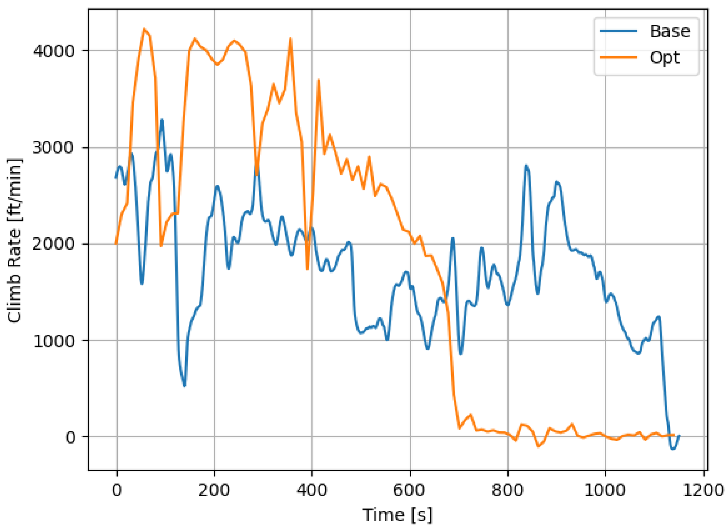
In this paper, we proposed a novel trajectory-optimization method that combines an artificial NN and GA. This approach enables optimization of the trajectory with any restrictions and flight envelope based on a precise fuel-consumption model of the trajectory. We utilized this method for the climbing phase of a Boeing 787. The optimization results indicated that it is desirable to climb continuously and rapidly to the cruise altitude at a faster rate of approximately 3000 ft/min compared to current practice, which could reduce fuel consumption by approximately 15%. Additionally, the trajectory plot showed that a vertical profile is possible under current airport operations, although it is difficult to handle overflight.

However, this method has some limitations that need to be considered. First, without constraints, the result goes out of the flight envelope, and the profile is impossible. This problem can be solved by improving the fuel-flow model. Second, the output solution is sometimes only locally optimal.

Our future research directions are as follows: First, we will incorporate weather conditions and arriving traffic into the simulation, verify the feasibility of safe implementation, and apply the optimized trajectory in practice. Second, we will use the optimized trajectory identified in this study to reduce overall fuel consumption at the airport. Finally, we will compare the convergence properties of different optimization algorithms while exploring the influence of various data sources, human factors, controllability, and passenger comfort.

References

1. International Air Transport Association (IATA). Industry Statistics Fact Sheet; International Air Transport Association (IATA): Montreal, QC, Canada, 2024. [Google Scholar]
2. Teoh, R.; Engberg, Z.; Schumann, U.; Voigt, C.; Shapiro, M.; Rohs, S.; Stettler, M. Global aviation contrail climate effects from 2019 to 2021. EGUsphere 2023, 2023, 1–32. [Google Scholar]
3. Stettler, M.E.; Boies, A.M.; Petzold, A.; Barrett, S.R. Global civil aviation black carbon emissions. Environ. Sci. Technol. 2013, 47, 10397–10404. [Google Scholar] [CrossRef]
4. Lee, D.S.; Fahey, D.W.; Skowron, A.; Allen, M.R.; Burkhardt, U.; Chen, Q.; Doherty, S.J.; Freeman, S.; Forster, P.M.; Fuglestvedt, J.; et al. The contribution of global aviation to anthropogenic climate forcing for 2000 to 2018. Atmos. Environ. 2021, 244, 117834. [Google Scholar] [CrossRef] [PubMed]
5. Villegas Díaz, M.; Gómez Comendador, V.F.; García-Heras Carretero, J.; Arnaldo Valdés, R.M. Environmental benefits in terms of fuel efficiency and noise when introducing continuous climb operations as part of terminal airspace operation. Int. J. Sustain. Transp. 2020, 14, 903–913. [Google Scholar] [CrossRef]
6. Wan, J.; Zhang, H.; Liu, F.; Lv, W.; Zhao, Y. Optimization of aircraft climb trajectory considering environmental impact under RTA constraints. J. Adv. Transp. 2020, 2020, 2738517. [Google Scholar] [CrossRef]
7. Zeh, T.; Lindner, M.; Rosenow, J.; Fricke, H. Optimization of departure routes beyond aircraft noise abatement. In Proceedings of the International Conference on Research in Air Transportation (ICRAT 2022), Tampa, FL, USA, 19–23 June 2022. [Google Scholar]
8. Ho-Huu, V.; Hartjes, S.; Visser, H.G.; Curran, R. An optimization framework for route design and allocation of aircraft to multiple departure routes. Transp. Res. Part D Transp. Environ. 2019, 76, 273–288. [Google Scholar] [CrossRef]
9. Zhang, M.; Huang, Q.; Liu, S.; Zhang, Y. Fuel-consumption model of the climbing phase of departure aircraft based on flight data analysis. Sustainability 2019, 11, 4362. [Google Scholar] [CrossRef]
10. Atipan, S.; Aerpanich, K. Fuel burn optimisation of jet-propelled aircraft during climb using excel solver. J. Aerosp. Soc. Malays. 2024, 2, 1–10. [Google Scholar]
11. Mori, R. Fuel-saving climb procedure by reduced thrust near top of climb. J. Aircr. 2020, 57, 800–806. [Google Scholar] [CrossRef]
12. Alexandrov, V.; Zybin, E.Y.; Kosyanchuk, V.; Selvesyuk, N.I.; Tremba, A.A.; Khlebnikov, M.V. Optimization of Aircraft Fuel Consumption During the Climb Phase. Autom. Remote Control 2022, 83, 1742–1757. [Google Scholar] [CrossRef]
13. Lindner, M.; Zeh, T.; Braßel, H.; Rosenow, J.; Fricke, H. Traffic flow funnels based on aircraft performance for optimized departure procedures. Future Transp. 2022, 2, 711–733. [Google Scholar] [CrossRef]
14. Miller, M.E.; Graham, M.; Aldous, J. Efficient climb and descent benefit pool. In Proceedings of the 2011 IEEE/AIAA 30th Digital Avionics Systems Conference, Seattle, WA, USA, 16–20 October 2011; pp. 2E1-1–2E1-11. [Google Scholar] [CrossRef]
15. Pérez-Castán, J.A.; Comendador, F.G.; Rodríguez-Sanz, A.; Montes, R.B.; Valdes, R.A.; Sanz, L.P. Impact of continuous climb operations on airport capacity. Transp. Res. Part C Emerg. Technol. 2018, 96, 231–250. [Google Scholar] [CrossRef]
16. Pérez-Castán, J.A.; Asensio, B.; Rodríguez-Sanz, Á.; Ho-Huu, V.; Sanz, L.P.; Comendador, F.G.; Valdés, R.M.A. Impact of continuous climb operations in ATC workload. Case-study Palma airport. J. Air Transp. Manag. 2020, 89, 101890. [Google Scholar] [CrossRef]
17. McNally, D.; Mueller, E.; Thipphavong, D.; Paielli, R.; Cheng, J.H.; Lee, C.; Sahlman, S.; Walton, J. A Near-Term Concept for Trajectory Based Operations with Air/Ground Data Link Communication. In Proceedings of the ICAS 2010, 27th Congress of the International Council of the Aeronautical Sciences, Nice, France, 19–24 September 2010. number ARC-E-DAA-TN2193. [Google Scholar]
18. Nuic, A.; Poles, D.; Mouillet, V. BADA: An advanced aircraft performance model for present and future ATM systems. Int. J. Adapt. Control Signal Process. 2010, 24, 850–866. [Google Scholar] [CrossRef]
19. Sun, J.; Hoekstra, J.M.; Ellerbroek, J. OpenAP: An open-source aircraft performance model for air transportation studies and simulations. Aerospace 2020, 7, 104. [Google Scholar] [CrossRef]
20. Poll, D.; Schumann, U. An estimation method for the fuel burn and other performance characteristics of civil transport aircraft in the cruise. Part 1 fundamental quantities and governing relations for a general atmosphere. Aeronaut. J. 2021, 125, 257–295. [Google Scholar] [CrossRef]
21. Poll, D.; Schumann, U. An estimation method for the fuel burn and other performance characteristics of civil transport aircraft during cruise: Part 2, determining the aircraft’s characteristic parameters. Aeronaut. J. 2021, 125, 296–340. [Google Scholar] [CrossRef]
22. Metlek, S. A new proposal for the prediction of an aircraft engine fuel consumption: A novel CNN-BiLSTM deep neural network model. Aircr. Eng. Aerosp. Technol. 2023, 95, 838–848. [Google Scholar] [CrossRef]
23. Uzun, M.; Demirezen, M.U.; Inalhan, G. Physics guided deep learning for data-driven aircraft fuel consumption modeling. Aerospace 2021, 8, 44. [Google Scholar] [CrossRef]
24. Baklacioglu, T. Modeling the fuel flow-rate of transport aircraft during flight phases using genetic algorithm-optimized neural networks. Aerosp. Sci. Technol. 2016, 49, 52–62. [Google Scholar] [CrossRef]
25. Chatterji, G.B. Fuel burn estimation using real track data. In Proceedings of the 11th AIAA Aviation Technology, Integration, and Operations (ATIO) Conference, Including the AIAA Balloon Systems Conference and 19th AIAA Lighter-Than, Virginia Beach, VA, USA, 20–22 September 2011; p. 6881. [Google Scholar]
26. Jarry, G.; Delahaye, D.; Hurter, C. Towards aircraft generic Quick Access Recorder fuel flow regression models for ADS-B data. In Proceedings of the International Conference on Research in Air Transportation, Singapore, 1–4 July 2024. [Google Scholar]
27. Senzig, D.A.; Fleming, G.G.; Iovinelli, R.J. Modeling of terminal-area airplane fuel consumption. J. Aircr. 2009, 46, 1089–1093. [Google Scholar] [CrossRef]
28. Clemons, E.; Reynolds, T.; Badrinath, S.; Chati, Y.; Balakrishnan, H. Enhancing aircraft fuel burn modeling on the airport surface. In Proceedings of the 2018 Aviation Technology, Integration, and Operations Conference, Atlanta, GA, USA, 25–29 June 2018; p. 3991. [Google Scholar]
29. Chati, Y.S.; Balakrishnan, H. Statistical modeling of aircraft engine fuel flow rate. In Proceedings of the 30th Congress of the International Council of the Aeronautical Science, Daejeon, Republic of Korea, 25–30 September 2016; pp. 1–10. [Google Scholar]
30. Karali, H.; Inalhan, G.; Tsourdos, A. Advanced UAV Design Optimization Through Deep Learning-Based Surrogate Models. Aerospace 2024, 11, 669. [Google Scholar] [CrossRef]
31. Lyu, Y.; Niu, Y.; He, T.; Shu, L.; Zhuravkov, M.; Zhou, S. An efficient method for the inverse design of thin-wall stiffened structure based on the machine learning technique. Aerospace 2023, 10, 761. [Google Scholar] [CrossRef]
32. Bakar, A.; Li, K.; Liu, H.; Xu, Z.; Alessandrini, M.; Wen, D. Multi-objective optimization of low reynolds number airfoil using convolutional neural network and non-dominated sorting genetic algorithm. Aerospace 2022, 9, 35. [Google Scholar] [CrossRef]
33. Abadi, M.; Agarwal, A.; Barham, P.; Brevdo, E.; Chen, Z.; Citro, C.; Corrado, G.S.; Davis, A.; Dean, J.; Devin, M.; et al. TensorFlow: Large-Scale Machine Learning on Heterogeneous Systems. 2015. Available online: http://www.tensorflow.org (accessed on 24 February 2025).
34. Fortin, F.A.; De Rainville, F.M.; Gardner, M.A.; Parizeau, M.; Gagné, C. DEAP: Evolutionary Algorithms Made Easy. J. Mach. Learn. Res. 2012, 13, 2171–2175. [Google Scholar]
35. Gotshall, S.; Rylander, B. Optimal population size and the genetic algorithm. Population 2002, 100, 900. [Google Scholar]
36. Federal Aviation Administration. Advisory Circular 25-13—Reduced and Derated Takeoff Thrust (Power) Procedures; Technical Report; U.S. Department of Transportation: Washington, DC, USA, 1988.
37. FAA Aviation Rulemaking Advisory Committee, Flight Test Harmonization Working Group. Topic 22 Derated/Reduced Takeoff Thrust Recommendation Report; Technical Report; U.S. Department of Transportation, Federal Aviation Administration: Washington, DC, USA, 2024.
38. Donaldson, R.; Fischer, D.; Gough, J.; Rysz, M. Economic impact of derated climb on large commercial engines. In Proceedings of the 2007 Boeing Performance and Flight Operations Engineering Conference; General Electric: Boston, MA, USA, 2007; p. 8-1. [Google Scholar]
39. Nakazawa, T.; Shinohara, N.; Hanaka, K. The effects of aircraft take-off thrust reduction on noise exposure around the airport. In Proceedings of the INTER-NOISE and NOISE-CON Congress and Conference Proceedings; Institute of Noise Control Engineering: Wakefield, MA, USA, 2019; Volume 259, pp. 7347–7352. [Google Scholar]
40. Koudis, G.S.; Hu, S.J.; Majumdar, A.; Jones, R.; Stettler, M.E. Airport emissions reductions from reduced thrust takeoff operations. Transp. Res. Part D Transp. Environ. 2017, 52, 15–28. [Google Scholar] [CrossRef]
Figure 1. Overview of this study; section numbers are shown in parentheses.
Aerospace 12 00583 g001
Figure 2. Trajectory definition and fuel burn calculation.
Aerospace 12 00583 g002
Figure 3. Structure of the NN; the inputs are the state of the aircraft, and the output is the current fuel flow.
Aerospace 12 00583 g003
Figure 4. Prediction without PR vs. actual value.
Aerospace 12 00583 g004
Figure 5. Prediction with PR vs. actual value.
Aerospace 12 00583 g005
Figure 6. Optimized trajectories in four trials; the numbers in the legend are the trial numbers.
Aerospace 12 00583 g006
Figure 7. Fitness value for generations; the numbers in the legend are the trial numbers (the trial numbers correspond to the trial numbers in Figure 6).
Aerospace 12 00583 g007
Figure 8. Sensitivity analysis of average fitness values with respect to mutation and crossover probabilities.
Aerospace 12 00583 g008
Figure 9. Optimized trajectories of Boeing 787; “Opt” is the optimized trajectory, and “Base” is an actual path of a flight.
Aerospace 12 00583 g009
Figure 10. Fuel flow vs. time.
Aerospace 12 00583 g010
Figure 11. Altitude vs. time.
Aerospace 12 00583 g011
Figure 12. True airspeed vs. time.
Aerospace 12 00583 g012
Figure 13. Climb speed vs. time.
Aerospace 12 00583 g013
Figure 14. Mach vs. time.
Aerospace 12 00583 g014
Figure 15. FPA vs. time.
Aerospace 12 00583 g015
Figure 16. Altitude vs. TAS.
Aerospace 12 00583 g016
Figure 17. Altitude vs. climb rate.
Aerospace 12 00583 g017
Figure 18. Altitude vs. Mach.
Aerospace 12 00583 g018
Figure 19. Altitude vs. FPA.
Aerospace 12 00583 g019
Figure 20. Fuel flow predicted by BADA and NN of the optimized trajectory and baseline actual data.
Aerospace 12 00583 g020