Satellite Navigation of a Lunar Rover with Sensor Fusion for High-Accuracy Navigation

Abstract

The Moon has become the focus of renewed interest for numerous space agencies and private companies worldwide. In the coming years, various scientific and commercial missions are planned, with a particular emphasis on exploring the South Pole. These missions include orbiters, landers, as well as both static and mobile rovers. For all these operations, continuous and accurate position knowledge is essential. This paper evaluates the performance of a navigation system designed for a lunar rover using the future satellite navigation infrastructure. It highlights the critical role of integrating multiple information sources, including a Digital Elevation Model (DEM) of the lunar surface and a high-precision Inertial Measurement Unit (IMU). The results demonstrate that a comprehensive suite of instruments enables highly accurate and reliable navigation for a mobile rover. While standalone satellite navigation, due to the reduced number of available sources, offers navigation accuracy of the orders of tens of meters, the addition of the DEM lowers the error at 5 m level; the IMU further improve by roughly 40% the performance on horizontal positioning.

1. Introduction

In recent years, interest in lunar exploration has surged, as NASA’s Artemis program [1] demonstrates, with the declared goal to return humans to the Moon.

To facilitate upcoming lunar operations, space agencies worldwide, in partnership with the private sector, are developing a dedicated communication and navigation network in lunar orbit. The European Space Agency (ESA) is advancing this effort through its Moonlight initiative [2], which aims to establish Lunar Communication and Navigation Services (LCNSs). By collaborating with commercial providers, the ESA seeks to enhance the capabilities available for both institutional and private lunar ventures.

The LCNS navigation framework draws inspiration from terrestrial GNSS, incorporating similar methodologies and technologies. It is based on the transmission of broadcast signals from LCNS satellites to predefined regions. These satellites will emit one-way signals while maintaining synchronization with each other and a common reference time scale. By processing the time of arrival and frequency of received CDMA (Code-Division Multiple-Access) signals, users can extract key navigation parameters—including pseudo-range, Doppler shift, and carrier phase—using broadcast navigation messages containing essential data such as ephemerides and clock corrections. With information from multiple LCNS satellites, users can independently compute their position, velocity, and the offset between their local receiver clock and the LCNS system reference time.

In this context, the one-way broadcast signal is also referred to as the Augmented Forward Signal (AFS), as defined in the Lunanet interoperability framework [3]. To maximize performance, LCNS is designed to be interoperable with Lunanet, allowing users to leverage multiple compatible navigation services, much like the multi-constellation approach used in terrestrial GNSS.

For effective navigation, users will need receivers capable of acquiring and tracking one-way signals from multiple LCNS satellites. However, given the technical constraints involved in deploying a full lunar navigation and communication constellation, the initial operational phase will likely include a limited number of satellites. As a result, standalone LCNS-based Position, Velocity, and Time (PVT) solutions may not always be sufficient to meet user requirements. To address this, PVT performance must be evaluated in conjunction with additional sensor integrations.

While previous works have focused on the case of a user orbiting the Moon [4], this paper presents an analysis of navigation performance for a mobile surface user, such as a lunar rover. Lunar rover navigation has been subject to many studies, focusing on different navigation techniques. Inertial navigation is for example considered in [5]. In ref. [6], the authors have developed crater-based localization to enable lunar rovers to estimate their global position and heading on the Moon with a goal performance of position error less than 5 m (m) and heading error less than 3 degree, 3σ, in sunlit areas. Visual odometry navigation is considered in [7], while position of a rover on surface of the Moon is suggested in [8] by using a group of self-calibrating rovers, which serves as mobile reference points. The present paper is specifically focused on the analysis of the performance that can be achieved using LCNS, examining the benefits of integrating complementary sensors, including an Inertial Measurement Unit (IMU) and a Digital Elevation Model (DEM), to enhance positioning accuracy and reliability. This study is currently under investigation by space agencies and research centers, as the works [9,10] show. In this research line, in [11] the use of an IMU is disregarded, while it is present in [10]. In this sense, the present work does not present novel or groundbreaking navigation algorithms, but it is aimed at serving as a benchmark for assessing the performance that can be expected for lunar rover navigation; specifically, this paper analyzes the relative importance of the different sensors, suggesting the best solution and a sub-optimal yet cost-effective solution. The convergence analysis is included to consolidate the performance assessment; finally, a Monte Carlo approach is implemented in order to have a reasonable estimate of the best accuracy that can be achieved by implementing the complete sensor suite. At the scope, a high-fidelity simulator of the available measurements (pseudorange, accelerations and local altitude information) is developed, as they serve as input for a loosely coupled Kalman Filter.

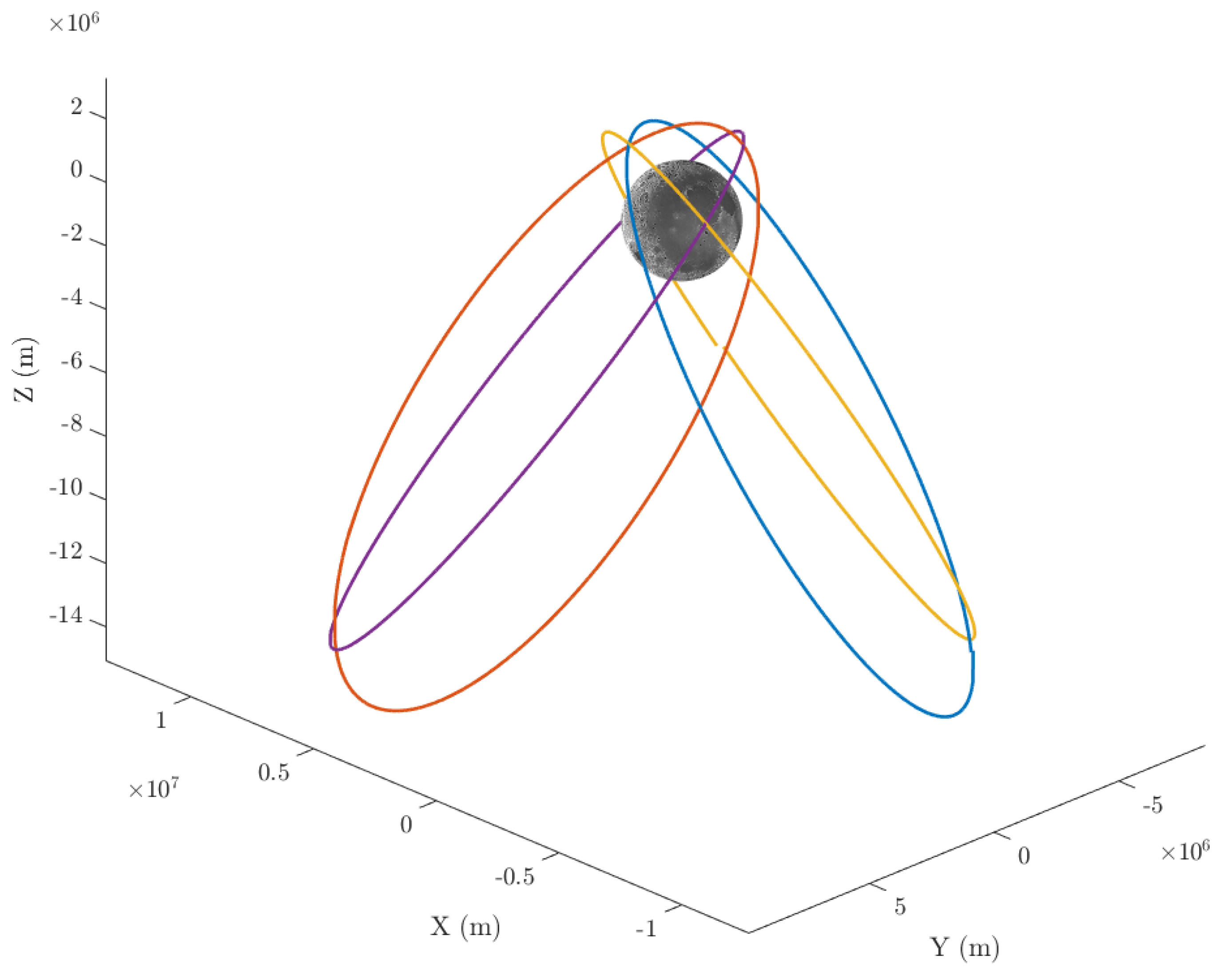
The paper is organized as follows: in Section 2, the scenario in terms of LCNS constellation and rover trajectory is described; the models of the sensors’ measurements are described in Section 3. The filter implementation, with all the modifications needed to include the different sensors, are described in Section 4 and Section 5. In Section 6 the impact of the inclusion of additional sensors is analyzed and discussed; in Section 7 a Monte Carlo approach has been implemented to statistically characterize the results, and in Section 8 the convergence time is studied. Final remarks are reported in Section 9.

2. Scenario

2.1. The ELFO Constellation

The considered LCNS navigation service is based on 4 navigation satellites with Eccentric Lunar Frozen Orbits (ELFOs).

The orbital parameters of the satellites of the candidate ELFO constellation for satellite navigation [12] are selected to provide high-stability, significant coverage of poles areas (in particular, the South Pole) while requiring low station-keeping budgets and minimizing orbit maintenance costs.

With respect to ref. [13] (where a constellation of 5 satellites was considered), in this work, four ELFO satellites in three different orbital planes are considered (as in [14]). This is a minimum for satellite navigation; thus, the performance obtained with this minimum configuration could only improve when larger constellations should be considered. The selected parameters are described in

Table 1. Initial ELFO osculating constellation parameters.

	SAT 1	SAT 2	SAT 3	SAT 4
a (km)	9748.997	9763.5	9740.5	9751.9
ecc	0.7	0.7	0.7	0.7
Incl (deg)	52.7	52.7	60	53
Arg (deg)	88.2	89.4	90.7	91.6
RAAN (deg)	−53.4	158.9	−18.9	129.9
f0 (deg)	188.4	158.3	4217.1	100.8

and the resulting orbits (propagated in a Moon Inertial frame t) are reported in Figure 1. The Moon Inertial frame, centered in the Moon, is defined as an inertial system referenced to the Moon equator (at the J2000 epoch) with the x-axis pointing along the line formed by the intersection of the Moon equator and Earth’s mean equator at J2000. The z-axis points along the Moon’s spin axis direction at the J2000 epoch. The y-axis completes the right-handed set.

2.2. Rover Trajectory

The rover’s trajectory is designed to traverse a crater, including both a descent and an ascent phase. The initial latitude and longitude are −88.319 deg and 78,456 deg, respectively, while the final latitude and longitude are −88.319 deg and 78.461 deg, respectively. The overall distance covered by the rover is 47.55 km during the 24 h. A 3D representation of the rover’s path can be found in Figure 2, while the altitude variation suffered during the travel is reported in Figure 3.

The most reasonable reference frame for the rover state representation and relevant estimation is a Moon-fixed reference frame. Two different systems have long been in use for the Moon [15]. These are the Mean Earth/polar axis, or often just Mean Earth (ME) and the Principal Axis systems. ME is defined by having 0° longitude in the mean direction of the Earth and an equator defined by the mean direction of the lunar rotation pole, and it is the current standard for mapping and defining surface coordinates. The PA is defined by the axes of the principal moments of inertia of the Moon [16,17], and it has been mostly used for modeling of geophysical parameters, such as the lunar gravity field.

The ME system has been employed for lunar mapping purposes for centuries, and there are many reasons to continue its use as the standard lunar coordinate system. The PA system is not more accurate and has no clear advantage over the ME system for mapping purposes. Following these considerations, the ME frame will be adopted.

3. Navigation Sensor Suite

3.1. LCNS Measurements

The pseudorange and the pseudorange rate measurements associated with the j-th satellite at epoch k can be modeled as

$${\widehat{\rho }}_{j,k}={\rho }_{j,k}+{\epsilon }_{j,k}$$

(1)

$${\widehat{\dot{\rho }}}_{j,k}={\dot{\rho }}_{j,k}+{\delta }_{j,k}$$

(2)

where ${\rho }_{j,k}$ and ${\dot{\rho }}_{j,k}$ represent the true values of the geometric range and the range rate referring to the j-th satellite at epoch k, whereas ${\epsilon }_{j,k}$ and ${\delta }_{j,k}$ are the pseudorange error and the pseudorange rate error.

3.1.1. Pseudorange

The pseudorange measurements are affected by various error source contributions including the satellite clock offset, multipath errors, user Delay Lock Loop (DLL) errors and the user clock offset. Each of these contributions is modeled and summed up to the simulated true range to obtain the pseudoranges. In particular, it shall be noted that the contribution of the satellite clock offset is subtracted rather than summed: this considers the fact that a delay in the satellite clock leads to an under-estimation on the pseudorange.

The satellite and users’ clocks have been modeled as miniRAFS and OCXO, respectively, according to [18,19].

The multipath effect is another important error source contribution that cannot be neglected in lunar scenarios. However, due to the lack of detailed and validated models for the estimation of lunar multipath effects, a simple Additive White Gaussian Noise (AWGN) model has been considered.

To model the user receiver thermal noise effects impacting the code tracking loop, assuming the user terminal implements a DLL, a general expression for the dynamic stress and the thermal noise code tracking error for a non-coherent DLL discriminator is reported in [20].

3.1.2. Pseudorange Rate

As thoroughly described in [20], the dominant sources of phase error in a navigation receiver Phase-Locked Loop (PLL) are thermal noise, oscillator imperfections, and dynamic stress. The phase error is the root sum square of every source of uncorrelated phase error such as thermal noise and oscillator noise. Oscillator noise includes vibration-induced error and Allan deviation-induced error. It also includes SV oscillator phase noise. However, rules of thumb can be used based on closed-form equations that approximate the measurement errors of the tracking loops, as presented in [20].

The time derivative of the estimated PLL error is then evaluated to compute the error contribution affecting the range rate measurements.

3.2. IMU Model

The IMU that is modeled for the lunar rover is a navigation grade device, for example the iMAR iNAV-RQH-1001 named in [10], where the linear acceleration is modeled using the following characteristic equation [21]:

$$y=\left[\begin{array}{ccc}{s}_x& {\epsilon }_{xy}& {\epsilon }_{xz}\\ {\epsilon }_{yx}& s_y& {\epsilon }_{yz}\\ {\epsilon }_{zx}& {\epsilon }_{zy}& s_z\end{array}\right]a+b+w$$

(3)

where $s_i$ are the scale factors on the three body axis, ${\epsilon }_{ij}$ are factors accounting for non-orthogonality, b is the vector of biases and w is the error of noise. All these terms are modeled as described in

Table 2. Characteristics of the modeled IMU.

IMU Parameter	Value
Frequency	10 Hz
Scale Factor Error Model	Gauss–Markov
Scale Factor Sigma	100 ppm
Scale Factor Correlation Time	7200 s
Bias Error Model	Gauss–Markov
Bias Sigma	10 $\mathsf{\mu }\mathrm{g}$
Bias Correlation Time	7200 s
Noise Error Model	Additive white Gaussian noise
Noise Sigma	8 ${\displaystyle \frac{\mathsf{\mu }\mathrm{g}}{\sqrt{\mathrm{H}\mathrm{z}}}}$
Orthogonality Error Model	Gauss–Markov
Orthogonality Sigma	0.025 (deg)
Orthogonality Correlation Time	7200 s

.

Because the focus of the paper is not on inertial navigation, in the following, some simplifications have been implemented. The measurement is not considered as coming from the IMU but is available from other sensors; of course, this means that the role of gyros in inertial navigation is neglected. The attitude is evaluated by the on-board computer at 1 Hz, with a 0.1-degree white gaussian noise affecting all rotation axes. The acceleration measurements can be rotated from the rover body-fixed frame to the Moon ME frame thanks to this additional source of information.

3.3. Digital Elevation Model

The DEM provides information about the altitude with respect to the reference Moon sphere (radius $R_{sphere}$ = 1737.4 km), given a certain latitude and longitude, and it provides a critical additional information for the rover navigation, even though DEM itself is affected by different sources of uncertainties: errors related to DEM data (due interpolation and orbital inaccuracies), errors due to terrain variations, and finally positional uncertainties of the rover itself [11]. The latter can significantly amplify altitude estimation errors, particularly around crater edges. The DEM used in this paper is produced by the Lunar Orbiter Laser Altimeter (LOLA) instrument on board the Lunar Reconnaissance Orbiter (LRO) [22].

This data product is a shape map (radius) of the Moon at a resolution of 10 m/pix by 10 m/pix, true at the pole in polar stereographic (spherical) projection, based on altimetry data acquired by the LOLA instrument. A visual representation of the used DEM in Figure 4. The dataset that can be found in [23] can be loaded on the navigation processor, but in order to implement a more realistic scenario, the position of the rover is based on a realization of the DEM that has been generated considering the original one and applying on top an error distribution to account for bias and noise on the source model, which differs from the expected one because of additional bias and noise.

The information from the DEM is extracted with the following approach: the latitude $\phi$ and longitude $\lambda$ of the rover are computed from the estimate state vector, considering the Moon as an ellipsoid with polar radius $R_p$ = 1736 km and equatorial radius $R_e$ = 1738.1 km.

The estimated position of the rover on the stereographic polar projection is computed:

$$\begin{array}{l}x=R_{sphere}\left({\displaystyle \frac{\pi }{2}}+\phi \right)\sin \left(\lambda \right)\\ x=R_{sphere}\left({\displaystyle \frac{\pi }{2}}+\phi \right)\cos \left(\lambda \right)\end{array}$$

The position in pixels on the DEM array is computed:

$$\begin{array}{l}{x}_{DEM}=-{\displaystyle \frac{y}{px}}+{\displaystyle \frac{D_{DEM}}{2}}\\ y_{DEM}={\displaystyle \frac{x}{px}}+{\displaystyle \frac{D_{DEM}}{2}}\end{array}$$

where in this case $px=10m$ is the pixel dimension and $D_{DEM}=15168$ is the dimension of the DEM array. A 2D interpolation is finally computed to find the altitude in correspondence to $x_{DEM}$, $y_{DEM}$.

4. Filter Implementation

4.1. Extended Kalman Filter Architecture

The basic architecture of the proposed navigation algorithms relies on the Extended Kalman Filter (EKF) approach. The details of the building blocks change according to the different scenarios as a function of the sensors that are included. In all cases, the EKF principle consists of a prediction phase, in which the current state is propagated from the previous one according to a dynamic model, followed by an update phase, in which the prediction is corrected thanks to the incoming measurements through an optimal gain called Kalman gain; associated with each quantity (estimate, prediction, measurement), there is a statistical information, the covariance matrix, that must be updated coherently. The loop is repeated iteratively (see Figure 5) starting from an initial guess. All the details can be found, for example, in ref. [24].

4.2. Propagation

The Kalman Filter assumed for the rover simulation implements in the state propagation stage a dynamic filter based on simple stationary dynamics, as no a priori knowledge of the rover trajectory is supposed to be available.

The estimate state vector is defined as:

$${\mathit{x}}_{r,0}={\left[x_r,y_r,z_r,{\dot{x}}_r,{\dot{y}}_r,{\dot{z}}_{r,},{\delta t}_r,{\dot{\delta t}}_r\right]}^T$$

where ${\left[x_r,y_r,z_r\right]}^T$ is the rover position, ${\left[{\dot{x}}_r,{\dot{y}}_r,{\dot{z}}_r\right]}^T$ is the rover velocity, and ${\left[{\delta t}_r,{\dot{\delta t}}_r\right]}^T$ is the rover receiver clock bias and clock bias drift. Position and velocity are expressed in the Moon ME frame. The initial error covariance 8 × 8 matrix ${\mathit{P}}_0$ associated to the state vector is defined as the expectation of the square of the deviation of the state vector estimate from the true value of the state vector:

$${\mathit{P}}_{\mathbf{0}}=\mathrm{d}\mathrm{i}\mathrm{a}\mathrm{g}{\left[\begin{array}{ccc}{\sigma }_{x,0}^2& {\sigma }_{y,0}^2& {\sigma }_{z,0}^2\end{array} \begin{array}{ccc}{\sigma }_{\dot{x},0}^2& {\sigma }_{\dot{y},0}^2& {\sigma }_{\dot{z},0}^2\end{array} \begin{array}{cc}{\sigma }_{\delta t,0}^2& {\sigma }_{\dot{\delta t},0}^2\end{array}\right]}^T$$

where ${\sigma }_{x,0}^2,{\sigma }_{y,0}^2,{\sigma }_{z,0}^2$ are variances in the position, ${\sigma }_{\dot{x},0}^2,{\sigma }_{\dot{y},0}^2,{\sigma }_{\dot{z},0}^2$ the velocity error variances, and ${\sigma }_{\delta t,0}^2 \mathrm{a}\mathrm{n}\mathrm{d} {\sigma }_{\dot{\delta t},0}^2$ the error variances of the receiver clock bias and clock bias drift. The following

Table 3. Initial elements of the state covariance matrix.

${\mathit{\sigma }}_{\mathit{x}0}$	${\mathit{\sigma }}_{\mathit{y}0}$	${\mathit{\sigma }}_{\mathit{z}0}$	${\mathit{\sigma }}_{\dot{\mathit{x}}0}$	${\mathit{\sigma }}_{\dot{\mathit{y}}0}$	${\mathit{\sigma }}_{\dot{\mathit{z}}0}$	${\mathit{\sigma }}_{\mathit{\delta }\mathit{t}0}$	${\mathit{\sigma }}_{\dot{\mathit{\delta }\mathit{t}}0}$
100 m	100 m	100 m	0.05 m/s	0.05 m/s	0.05 m/s	100 m	0.05 m/s

shows the standard deviation values used in the simulation to define the initial state covariance matrix.

The rover state vector and the associated error covariance matrix estimated at epoch k − 1 is propagated to the epoch k:

$${\widehat{\mathit{x}}}_{k|k-1}={\mathit{\Phi }}_{k-1}{\widehat{\mathit{x}}}_{k-1|k-1}$$

(4)

$${\mathit{P}}_{k|k-1}={\mathit{\Phi }}_{k-1}{\mathit{P}}_{k-1|k-1}{\mathit{\Phi }}_{k-1}^T+{\mathit{Q}}_{k-1}$$

(5)

where ${\widehat{\mathit{x}}}_{k|k-1}$ and ${\mathit{P}}_{k|k-1}$ are, respectively, the state vector and the relative error covariance matrix propagated at epoch k with the measurements available at epoch k − 1. $\mathit{\Phi }$ is the transition matrix:

$${\Phi }_{k-1}=\left[\begin{array}{cccc}{I}^{3\times 3}& dt\cdot I^{3\times 3}& 0^{3\times 1}& 0^{3\times 1}\\ 0^{3\times 3}& I^{3\times 3}& 0^{3\times 1}& 0^{3\times 1}\\ 0^{1\times 3}& 0^{1\times 3}& 1& dt\\ 0^{1\times 3}& 0^{1\times 3}& 0& 1\end{array}\right]$$

(6)

$0^{n\times m},I^{n\times m}$ are the zero matrix and the identity matrix of dimensions $\left(n\times m\right)$, respectively.

Q_k is the process noise covariance matrix referring to the inaccuracies assumed for the propagation model, described at each t_k time by the following matrix, with values as per

Table 4. Elements of the process disturbances’ covariance matrix.

${\mathit{\sigma }}_{\mathit{x}}$	${\mathit{\sigma }}_{\mathit{y}}$	${\mathit{\sigma }}_{\mathit{z}}$	${\mathit{\sigma }}_{\dot{\mathit{x}}}$	${\mathit{\sigma }}_{\dot{\mathit{y}}}$	${\mathit{\sigma }}_{\dot{\mathit{z}}}$	${\mathit{\sigma }}_{\mathit{\delta }\mathit{t}}$	${\mathit{\sigma }}_{\dot{\mathit{\delta }\mathit{t}}}$
1 m	1 m	1 m	0.1 m/s	0.1 m/s	0.1 m/s	1 m	1 × 10−5 m/s

:

$${\mathit{Q}}_{\mathit{k}}=\mathrm{d}\mathrm{i}\mathrm{a}\mathrm{g}{\left[ \begin{array}{ccc}{\sigma }_x^2& {\sigma }_y^2& {\sigma }_z^2\end{array} \begin{array}{ccc}{\sigma }_{\dot{x}}^2& {\sigma }_{\dot{y}}^2& {\sigma }_{\dot{z}}^2\end{array} \begin{array}{cc}{\sigma }_{\delta t}^2& {\sigma }_{\dot{\delta t}}^2\end{array}\right]}^T$$

(7)

4.3. State Update

Once the pseudorange and pseudorange rate measurements are available at epoch k together with the propagated state and associated error covariance matrix, then the Kalman gain ${\mathit{K}}_k$, minimizing the trace of the error covariance matrix of the estimates, can be computed:

$${\mathit{K}}_k={\mathit{P}}_{k|k-1}{\mathit{H}}_k^T{\left({\mathit{H}}_k{\mathit{P}}_{k|k-1}{\mathit{H}}_k^T+{\mathit{R}}_k\right)}^{-1}$$

(8)

where ${\mathit{H}}_k$ is the measurement matrix and ${\mathit{R}}_k$ is the error covariance matrix of the measurements. The propagated state vector and the associated error covariance matrix can be finally updated for the next iteration as:

$${\widehat{\mathit{x}}}_{k|k}={\widehat{\mathit{x}}}_{k|k-1}+{\mathit{K}}_k({\mathit{z}}_k-{\mathit{z}}_{p,k})$$

(9)

$${\mathit{P}}_{k|k}=\left(\mathit{I}-{\mathit{K}}_k{\mathit{H}}_k\right){\mathit{P}}_{k|k-1}{\left(\mathit{I}-{\mathit{K}}_k{\mathit{H}}_k\right)}^T+{\mathit{K}}_k{\mathit{R}}_k{\mathit{K}}_k^T$$

(10)

where ${\mathit{z}}_{p,k}$ is the prediction of the measurements, computed following the measurement equations as described in the following paragraph (in particular, Equations (18) and (19)).

5. Measurements

5.1. Satellite Navigation

The measurement vector containing the pseudorange and the pseudorange rate measurements from m satellites at epoch k can be defined as

$${\mathit{z}}_k={\left[{\rho }_{1,k},{\rho }_{2,k},\dots ,{\rho }_{m,k},{\dot{\rho }}_{1,k},{\dot{\rho }}_{2,k},\dots ,{\dot{\rho }}_{m,k}\right]}^T$$

(11)

where ${\rho }_{j,k}$ and ${\dot{\rho }}_{j,k}$ are, respectively, the estimated pseudorange and pseudorange rate measurements referring to the j-th satellite with j = 1, …, m. The measurement error covariance matrix is computed as:

$${\mathit{R}}_k={\mathit{T}}_{corr}\left[\begin{array}{cc}{\mathit{R}}_{yy}& 0\\ 0& {\mathit{R}}_{cc}\end{array}\right]{\mathit{T}}_{corr}^T$$

(12)

where ${\mathit{T}}_{corr}$ is

$${\mathit{T}}_{corr}=\left[\begin{array}{cccccc}{\mathit{I}}_m& 0& -\mathit{U}& 0& {\mathit{I}}_m& 0\\ 0& {\mathit{I}}_m& 0& -\mathit{U}& 0& {\mathit{I}}_m\end{array}\right]$$

(13)

with $\mathit{U}=\left[\begin{array}{ccc}{\widehat{r_1}}^T& 0& 0\\ 0& \dots & 0\\ 0& 0& {\widehat{r_m}}^T\end{array}\right]$,${\widehat{r}}_j={\displaystyle \frac{1}{{\Vert r\Vert }_j}}\left[\begin{array}{c}(x_j-x)\\ \left(y_j-y\right)\\ \left(z_j-z\right)\end{array}\right]$ and ${\mathit{R}}_{yy}$ being the error covariance matrix associated with the tracking error contribution:

$${\mathit{R}}_{yy}=\left[\begin{array}{cccccc}{\sigma }_{DLL1}^2& 0& 0& 0& 0& 0\\ 0& \dots & 0& 0& 0& 0\\ 0& 0& {\sigma }_{DLLm}^2& 0& 0& 0\\ 0& 0& 0& {\sigma }_{FLL1}^2& 0& 0\\ 0& 0& 0& 0& \dots & 0\\ 0& 0& 0& 0& 0& {\sigma }_{FLLm}^2\end{array}\right]$$

(14)

where ${\sigma }_{DLLj}$ and ${\sigma }_{FLLj}$ (with specific values used in the tracking jitter expressions reported in

Table 5. Receiver tracking measurement model.

LCNS Receiver Parameters
DLL Loop bandwidth (BDLL)	1 Hz
FLL Loop bandwidth (BFLL)	2 Hz
Coherent integration (Ti)	16 ms
Early-late spacing (d)	0.25 chip
Wavelength (λ)	14.28 cm
Chip length (λC)	29.305 m
Factor (F)	2

) are the error standard deviations associated with the pseudorange and pseudorange rate measurements corresponding to the j-th satellite, respectively:

$${\sigma }_{DLL}={\lambda }_C\sqrt{{\displaystyle \frac{B_{L}d}{2CN0}}\left(1+{\displaystyle \frac{1}{T_{i}CN0}}\right)}, {\sigma }_{FLL}={\displaystyle \frac{{\lambda }_L}{2\pi T_i}}\sqrt{{\displaystyle \frac{4F{B}_{FLL}}{CN0}}\left(1+{\displaystyle \frac{1}{T_{i}CN0}}\right)}$$

(15)

${\mathit{R}}_{cc}$ is the error covariance matrix associated with the LCNS navigation message parameters:

$${\mathit{R}}_{\mathit{c}\mathit{c}=}=\mathrm{d}\mathrm{i}\mathrm{a}\mathrm{g}{\left[\begin{array}{ccc}{\sigma }_{{x,s}_1}^2& {\sigma }_{{y,s}_1}^2& {\sigma }_{{z,s}_1}^2\end{array} \begin{array}{ccc}\dots & {\sigma }_{{x,s}_m}^2& {\sigma }_{{y,s}_m}^2\end{array} \begin{array}{ccc} \begin{array}{ccc}{\sigma }_{{z,s}_m}^2& {\sigma }_{{\dot{x}}_{s_1}}^2& \dots \end{array} {\sigma }_{{\dot{x}}_{s_m}}^2& {\sigma }_{t_{s_1}}^2& \dots \end{array} \begin{array}{ccc}{\sigma }_{t_{s_m}}^2& {\sigma }_{{\dot{t}}_{s_m}}^2& \dots \end{array} {\sigma }_{{\dot{t}}_{s_m}}^2 \right]}^T$$

(16)

where ${\sigma }_{{x,s}_j}^2,{\sigma }_{{y,s}_j}^2,{\sigma }_{{z,s}_j}^2$ are the error variances in the position of the j-th satellite, ${\sigma }_{{\dot{x}}_{s_j}}^2,{\sigma }_{{\dot{y}}_{s_j}}^2,{\sigma }_{{\dot{z}}_{s_j}}^2$ are the error variances in the velocity of the j-th satellite, and ${\sigma }_{t_{s_j}}^2$ and ${\sigma }_{{\dot{t}}_{s_j}}^2$ are the error variances of the satellite clock and satellite clock drift, respectively.

Table 6. LCNS satellites’ orbits and clocks measurement models (1σ).

Error Variance Component	Value
${\sigma }_{xs}$	2.89 m
${\sigma }_{ys}$	2.89 m
${\sigma }_{zs}$	2.89 m
${\sigma }_{\dot{x}s}$	0.00075 m/s
${\sigma }_{\dot{y}s}$	0.00075 m/s
${\sigma }_{\dot{z}s}$	0.00075 m/s
${\sigma }_{\delta ts}$	7.5 m
${\sigma }_{\dot{\delta t}s}$	0.00075 m/s

reports the error standard deviations associated with the position and velocity of each LCNS satellite and the error standard deviations of the satellite clock and clock drift considered in the simulation exercise.

In this case, the only measurements available on board are the pseudoranges, which can be 4 or less according to the ELFO satellites visible by the orbiter. Let us consider the position and the velocity of the j-th satellite in the Moon Inertial frame at epoch k:

$${\mathit{x}}_{s_j,k}={\left[x_{s_j,k},y_{s_j,k},z_{s_j,k},{\dot{x}}_{s_j,k},{\dot{y}}_{s_j,k},{\dot{z}}_{s_j,k}\right]}^T$$

(17)

The pseudorange and the pseudorange rate between the user and the j-th satellite are defined as follows:

$${\rho }_{\mathrm{j},\mathrm{k}}=\sqrt{{\left(x_{s_j,k}-x_{r,k}\right)}^2+{\left(y_{s_j,k}-y_{r,k}\right)}^2+{\left(z_{s_j,k}-z_{r,k}\right)}^2}+{\delta t}_{r,k}$$

(18)

$$\begin{gathered} {\dot{\rho }}_{j,k}={\displaystyle \frac{\left(x_{s_j,k}-x_{r,k}\right)}{r_j}}{(\dot{x}}_{s_1,k}-{\dot{x}}_{r,k})+{\displaystyle \frac{\left(y_{s_j,k}-y_{r,k}\right)}{r_j}}{(\dot{y}}_{s_1,k}-{\dot{y}}_{r,k})+ \\ {\displaystyle \frac{\left(z_{s_j,k}-z_{r,k}\right)}{r_j}}{(\dot{z}}_{s_1,k}-{\dot{z}}_{r,k})+{\dot{\delta t}}_{r,k} \end{gathered}$$

(19)

The linearization of the pseudorange and the pseudorange rate results in

$$∆{\mathit{z}}_k={\mathit{H}}_k{∆\mathit{x}}_{r,k}$$

(20)

where $∆{\mathit{z}}_k$ is the increment in the pseudorange and the pseudorange rate, ${∆\mathit{x}}_{r,k}$ is the increment in the state vector, and ${\mathit{H}}_k$ is the geometric matrix at time k:

$$∆{\mathit{z}}_k={\left[∆{\rho }_{1,k},∆{\rho }_{2,k},\dots ,∆{\rho }_{m,k},∆{\dot{\rho }}_{1,k},∆{\dot{\rho }}_{2,k},\dots ,∆{\dot{\rho }}_{m,k}\right]}^T$$

(21)

$${∆\mathit{x}}_{r,k}={\left[∆x_{r,k},∆y_{r,k},∆z_{r,k},∆{\dot{x}}_{r,k},∆{\dot{y}}_{r,k},∆{\dot{z}}_{r,k},∆{\delta t}_{r,k},∆{\dot{\delta t}}_{r,k}\right]}^T$$

(22)

$${\mathit{H}}_k=\left[\begin{array}{cccccccc}-{\displaystyle \frac{x_{s_1,k}-x_{r,k}}{r_1}}& -{\displaystyle \frac{y_{s_1,k}-y_{r,k}}{r_1}}& -{\displaystyle \frac{z_{s_1,k}-z_{r,k}}{r_1}}& 0& 0& 0& 1& 0\\ -{\displaystyle \frac{x_{s_2,k}-x_{r,k}}{r_2}}& -{\displaystyle \frac{y_{s_2,k}-y_{r,k}}{r_2}}& -{\displaystyle \frac{z_{s_1,k}-z_{r,k}}{r_1}}& 0& 0& 0& 1& 0\\ :& :& :& :& :& :& :& :\\ :& :& :& :& :& :& :& :\\ -{\displaystyle \frac{x_{s_m,k}-x_{r,k}}{r_m}}& -{\displaystyle \frac{y_{s_m,k}-y_{r,k}}{r_m}}& -{\displaystyle \frac{z_{s_m,k}-z_{r,k}}{r_m}}& 0& 0& 0& 1& 0\\ -{\displaystyle \frac{{(\dot{x}}_{s_1,k}-{\dot{x}}_{r,k})}{r_1}}+{\displaystyle \frac{\left(x_{s_1,k}-x_{r,k}\right)}{r_1^2}}{\dot{r}}_1& -{\displaystyle \frac{{(\dot{y}}_{s_1,k}-{\dot{y}}_{r,k})}{r_1}}+{\displaystyle \frac{\left(y_{s_1,k}-y_{r,k}\right)}{r_1^2}}{\dot{r}}_1& -{\displaystyle \frac{{(\dot{z}}_{s_1,k}-{\dot{z}}_{r,k})}{r_1}}+{\displaystyle \frac{\left(z_{s_1,k}-z_{r,k}\right)}{r_1^2}}{\dot{r}}_1& -{\displaystyle \frac{x_{s_1,k}-x_{r,k}}{r_1}}& -{\displaystyle \frac{y_{s_1,k}-y_{r,k}}{r_1}}& -{\displaystyle \frac{z_{s_1,k}-z_{r,k}}{r_1}}& 0& 1\\ -{\displaystyle \frac{{(\dot{x}}_{s_2,k}-{\dot{x}}_{r,k})}{r_2}}+{\displaystyle \frac{\left(x_{s_2,k}-x_{r,k}\right)}{r_2^2}}{\dot{r}}_2& -{\displaystyle \frac{{(\dot{y}}_{s_2,k}-{\dot{y}}_{r,k})}{r_2}}+{\displaystyle \frac{\left(y_{s_2,k}-y_{r,k}\right)}{r_2^2}}{\dot{r}}_2& -{\displaystyle \frac{{(\dot{z}}_{s_1,k}-{\dot{z}}_{r,k})}{r_1}}+{\displaystyle \frac{\left(z_{s_1,k}-z_{r,k}\right)}{r_1^2}}{\dot{r}}_1& -{\displaystyle \frac{x_{s_2,k}-x_{r,k}}{r_2}}& -{\displaystyle \frac{y_{s_2,k}-y_{r,k}}{r_2}}& -{\displaystyle \frac{z_{s_1,k}-z_{r,k}}{r_1}}& 0& 1\\ :& :& :& :& :& :& :& :\\ :& :& :& :& :& :& :& :\\ -{\displaystyle \frac{{(\dot{x}}_{s_m,k}-{\dot{x}}_{r,k})}{r_m}}+{\displaystyle \frac{\left(x_{s_m,k}-x_{r,k}\right)}{r_m^2}}{\dot{r}}_m& -{\displaystyle \frac{{(\dot{y}}_{s_m,k}-{\dot{y}}_{r,k})}{r_m}}+{\displaystyle \frac{\left(y_{s_m,k}-y_{r,k}\right)}{r_m^2}}{\dot{r}}_m& -{\displaystyle \frac{{(\dot{z}}_{s_1,k}-{\dot{z}}_{r,k})}{r_1}}+{\displaystyle \frac{\left(z_{s_1,k}-z_{r,k}\right)}{r_1^2}}{\dot{r}}_1& -{\displaystyle \frac{x_{s_m,k}-x_{r,k}}{r_m}}& -{\displaystyle \frac{y_{s_m,k}-y_{r,k}}{r_m}}& -{\displaystyle \frac{z_{s_1,k}-z_{r,k}}{r_1}}& 0& 1\end{array}\right]$$

(23)

5.2. DEM

In the rover scenario, the measurements can be enriched by the information provided by the DEM. This means that the measurement vector is increased by one element:

$$∆{\mathit{z}}_k={\left[∆{\rho }_{1,k},∆{\rho }_{2,k},\dots ,∆{\rho }_{m,k},∆{\dot{\rho }}_{1,k},∆{\dot{\rho }}_{2,k},\dots ,∆{\dot{\rho }}_{m,k},h\right]}^T$$

(24)

where h is computed as described in Section 3.3. Consequently, the measurement matrix is also increased by one last row, which reads as:

$$\begin{array}{c}{H}_k^h={\left.{\displaystyle \frac{\partial h}{\partial x}}\right|}_{x={\widehat{x}}_{k|k-1}}\hfill \\ =\left[\begin{array}{cccccccc}{\displaystyle \frac{x_r}{\sqrt{\left(x_r^2+y_r^2+z_r^2\right)}}}& {\displaystyle \frac{y_r}{\sqrt{\left(x_r^2+y_r^2+z_r^2\right)}}}& {\displaystyle \frac{z_r}{\sqrt{\left(x_r^2+y_r^2+z_r^2\right)}}}& 0& 0& 0& 0& 0\end{array}\right]\hfill \end{array}$$

(25)

Therefore, the assembled measurement matrix can be defined as

$$H_k^{LCNS+DEM}=\left[\begin{array}{c}{H}_k\\ H_k^h\end{array}\right]$$

(26)

with H_k being the measurement matrix defined for the LCNS case, i.e., when only the pseudorange and pseudorange rates are available. The error covariance matrix of the measurements for the lander/rover case becomes:

$$R_k^{LCNS+DEM}=\left[\begin{array}{cc}{R}_k& 0\\ 0& {\sigma }_{v_h}^2\end{array}\right]$$

(27)

where ${\sigma }_{v_h}^2$ is the variance of DEM information. For the simulations, a Gauss–Markov process is adopted for describing the DEM error, with:

$${\sigma }_{v_h}^2={\sigma }_{DEM}^2(1-e^{{\displaystyle \frac{ho{r}_{err}}{DE{M}_{corr}}}})$$

(28)

${\sigma }_{DEM}$= 20 m, $DE{M}_{corr}=10$, and $ho{r}_{err}$ is the estimated error in the horizontal plane, computed from the elements of the state covariance matrix. Here and in the following, the term horizontal refers to a plane that is orthogonal to the vector from the Moon center to the rover position.

5.3. IMU

In order to keep the additional possible sensors as decoupled as possible from the main navigation system, i.e., the LCNS, a loosely coupled architecture is selected for this study.

According to this design, a second Kalman Filter (here named the INS filter) must be implemented, which integrates the IMU accelerations at the IMU data rate (10 Hz) and takes the EKF estimates (position and velocity) as measurements. The prediction and update steps of the Kalman Filter are the same as described in Section 4, and they will not be repeated here; it is sufficient here to say that the dynamic model for position is a double integrator, while the bias, once rotated in the rover body frame, is supposed to have a constant dynamic. Differently from the LCNS filter, here, the estimate state comprises the position, the velocity, and IMU biases, which are the only characteristics of the IMU that will be explicitly estimated.

The prediction phase is performed at 10 Hz, while the update phase is computed at 1 Hz, i.e., when a new estimate from the LCNS filter is available. In fact, the LCNS estimates are input as measurements to the integration Kalman Filter [24].

The overall architecture in this case is depicted in Figure 6.

It must be noted that different navigation algorithms could be used: the Unscented Kalman Filter, as an example, could be implemented instead of the EKF; the fusion of IMU and LCNS measurements could be performed with more coupled architectures (tightly coupled or deeply coupled architectures; see [24] again). The architecture proposed in this paper is maybe one of the simplest and lighter from the computational point of view, which represents an issue for on-board implementation. Even though a test on a flight hardware replica is not among the objectives of this study, an idea of the computation load can be obtained by measuring the computation time of a single step of the navigation loop on a normal desktop PC (13th Gen Intel(R) Core(TM) i9-13900K, 3.00 GHz processor, 64 GB RAM), which is, as a mean, $1.6 {10}^{-4}$ s. This can be considered a promising value for real-time implementation.

6. Simulation Results: Analysis of Sensors Contribution

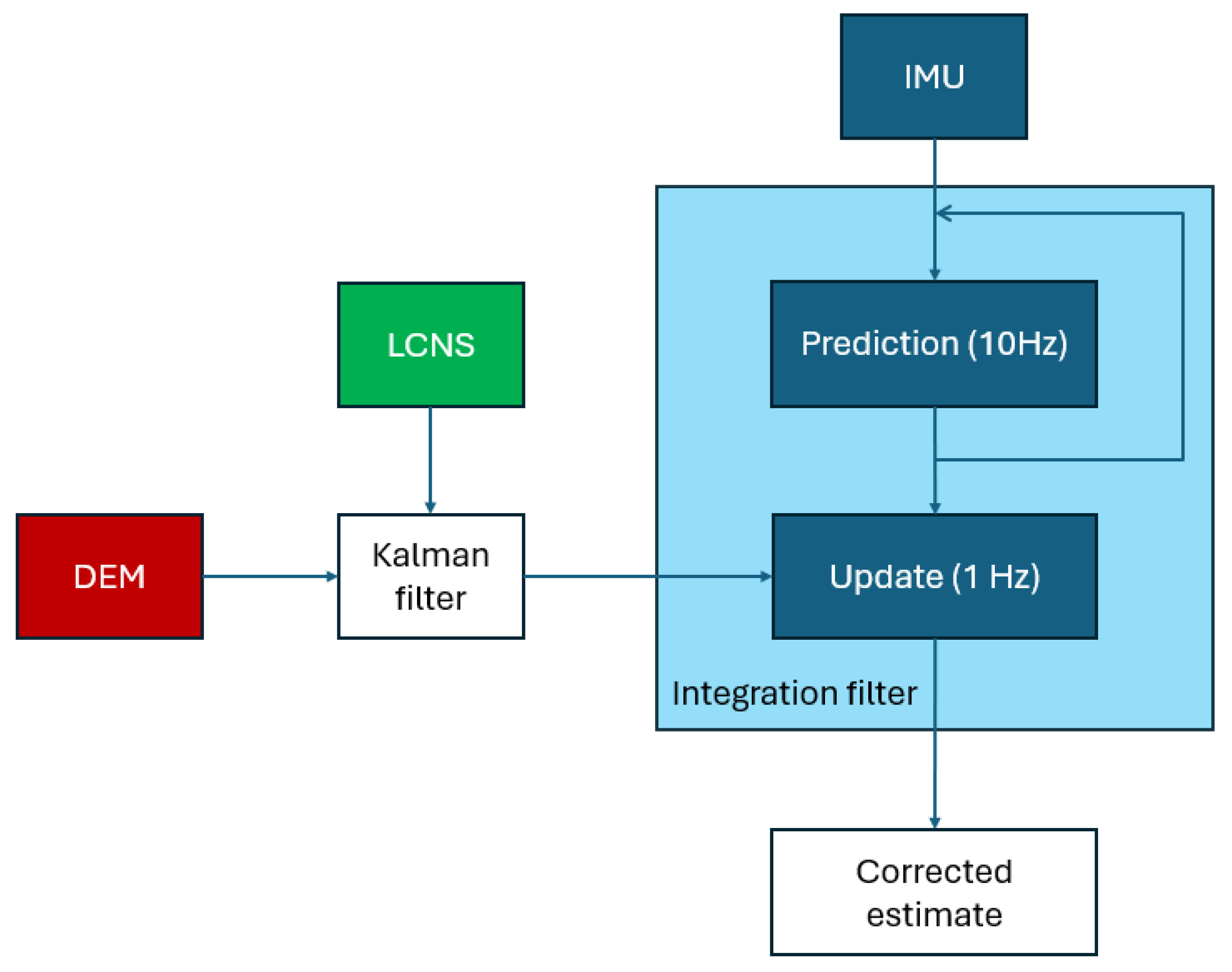
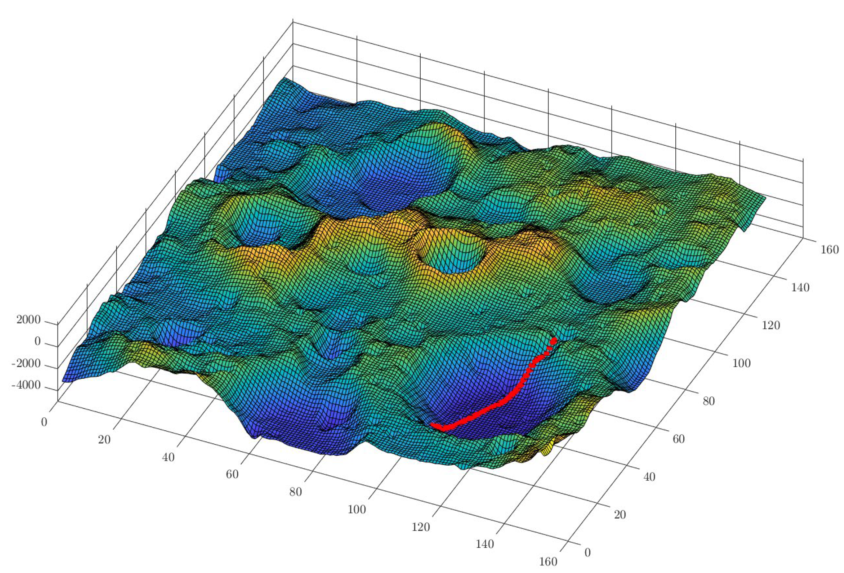
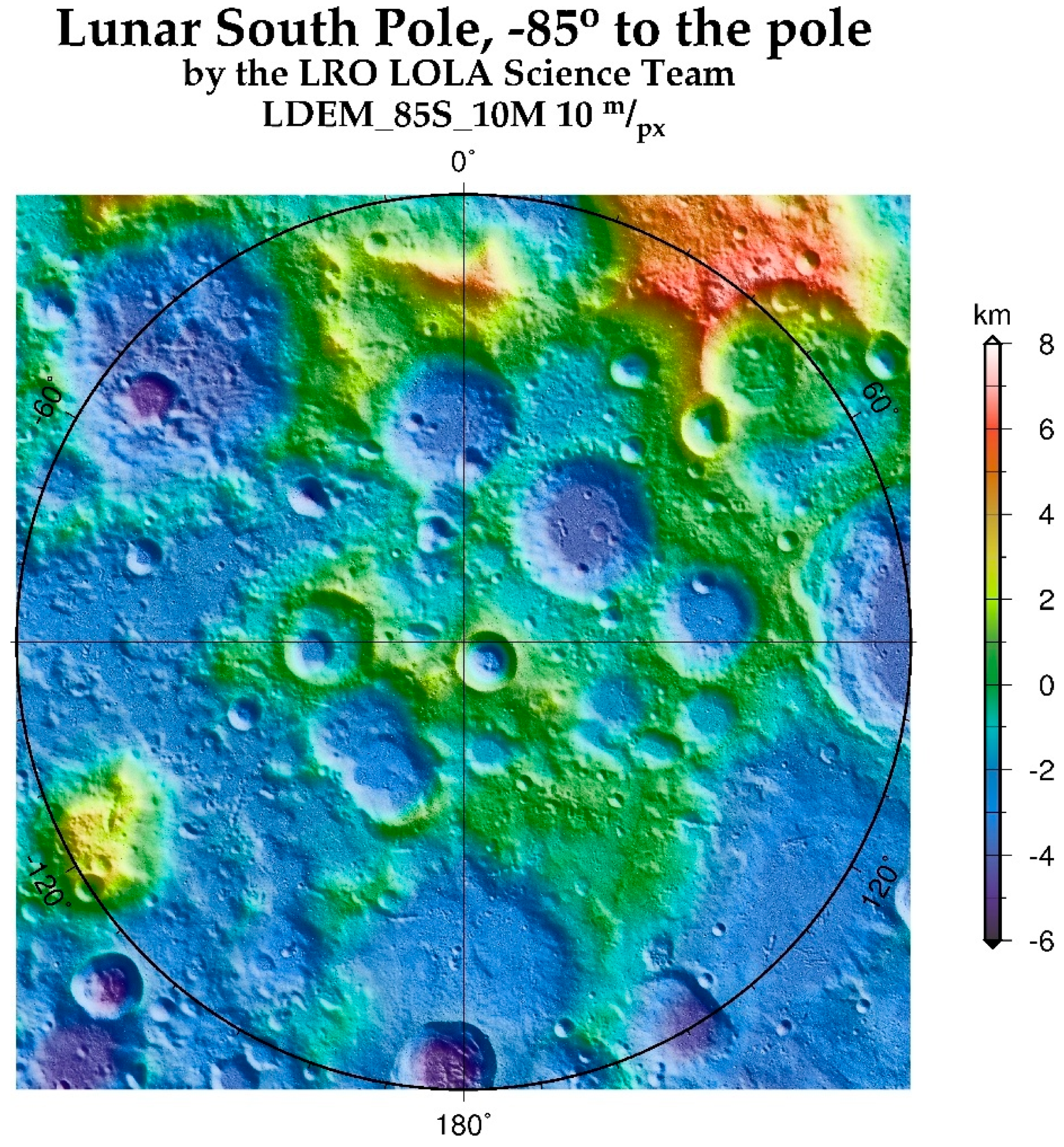
In order to run the simulations, the architecture reported in Figure 7 is implemented. The ground truth is realized by taking into account a high-precision propagation of the satellite state (using System Tool Kit 12 software) and the realization of the DEM (derived—but not coincident—with the data in [23]); the sensors models provides the noisy measurements from LCNS satellites, DEM, and IMU, which can be used (or not, according to the cases) as input to the navigation filter.

In this first analysis, the focus is on the performance of PVT algorithm when stationary. Therefore, the initial conditions are considered perfectly known. The convergence time will be analyzed in a separate case study (Section 8).

For this scenario, the percentage of time in which a number j satellites are in view is reported in

Table 7. Percentage of time in which a number N of satellites are in view (from 0 to 4).

${\mathit{P}}_{\mathit{v}\mathit{i}\mathit{e}\mathit{w}0}$	${\mathit{P}}_{\mathit{v}\mathit{i}\mathit{e}\mathit{w}1}$	${\mathit{P}}_{\mathit{v}\mathit{i}\mathit{e}\mathit{w}2}$	${\mathit{P}}_{\mathit{v}\mathit{i}\mathit{e}\mathit{w}3}$	${\mathit{P}}_{\mathit{v}\mathit{i}\mathit{e}\mathit{w}4}$
0.0%	0.00%	0.00%	64.10%	35.90%

.

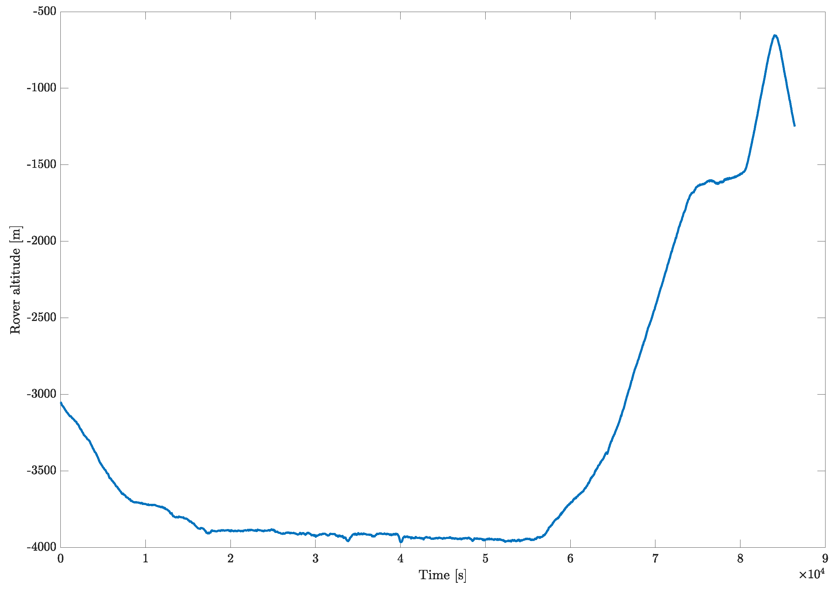
The simulation time span is one day (86,400 s), with the initial date fixed at 1 January 2027. The time step is 1 s for LCNS and DEM information, while it is 0.1 s for the IMU.

The estimated state, in terms of position, velocity, and time, is compared with the true state for four different sensor suites, combining the availability of the satellite navigation (as a baseline), the DEM, the IMU, and all three information sources.

6.1. LCNS—Standalone

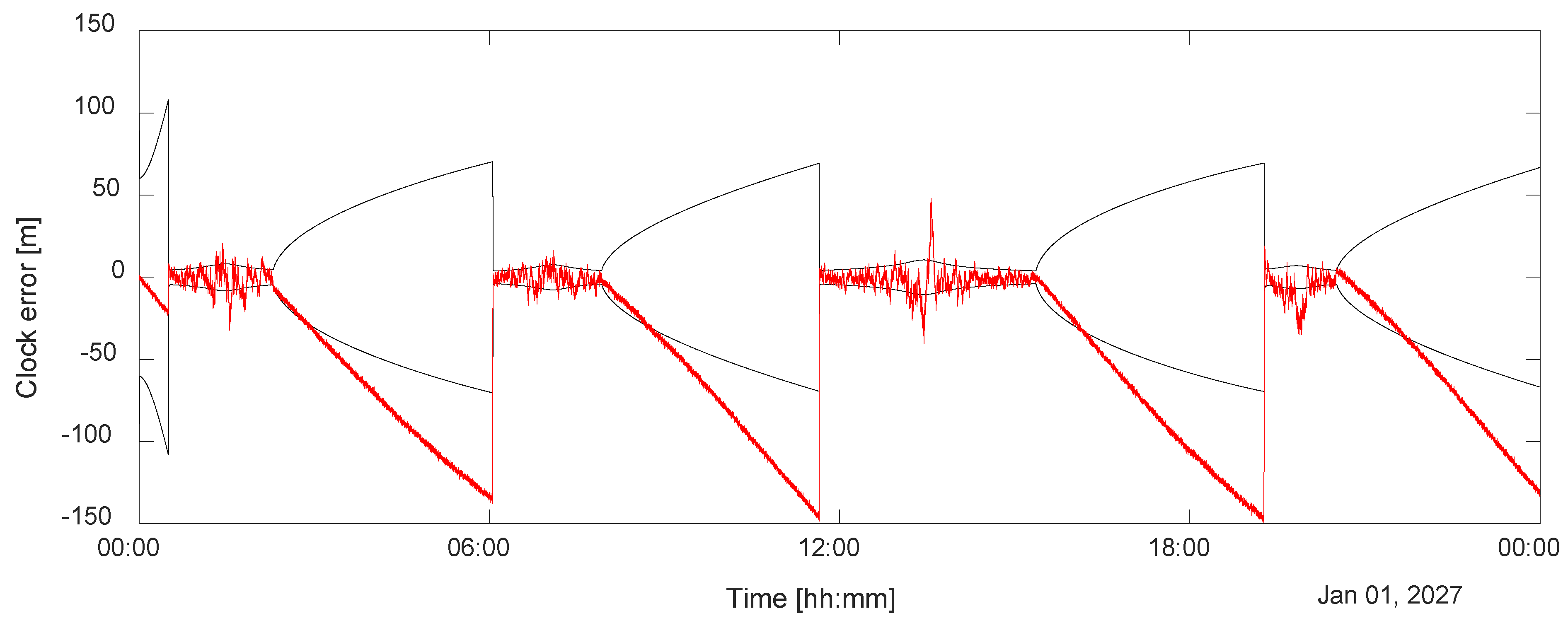
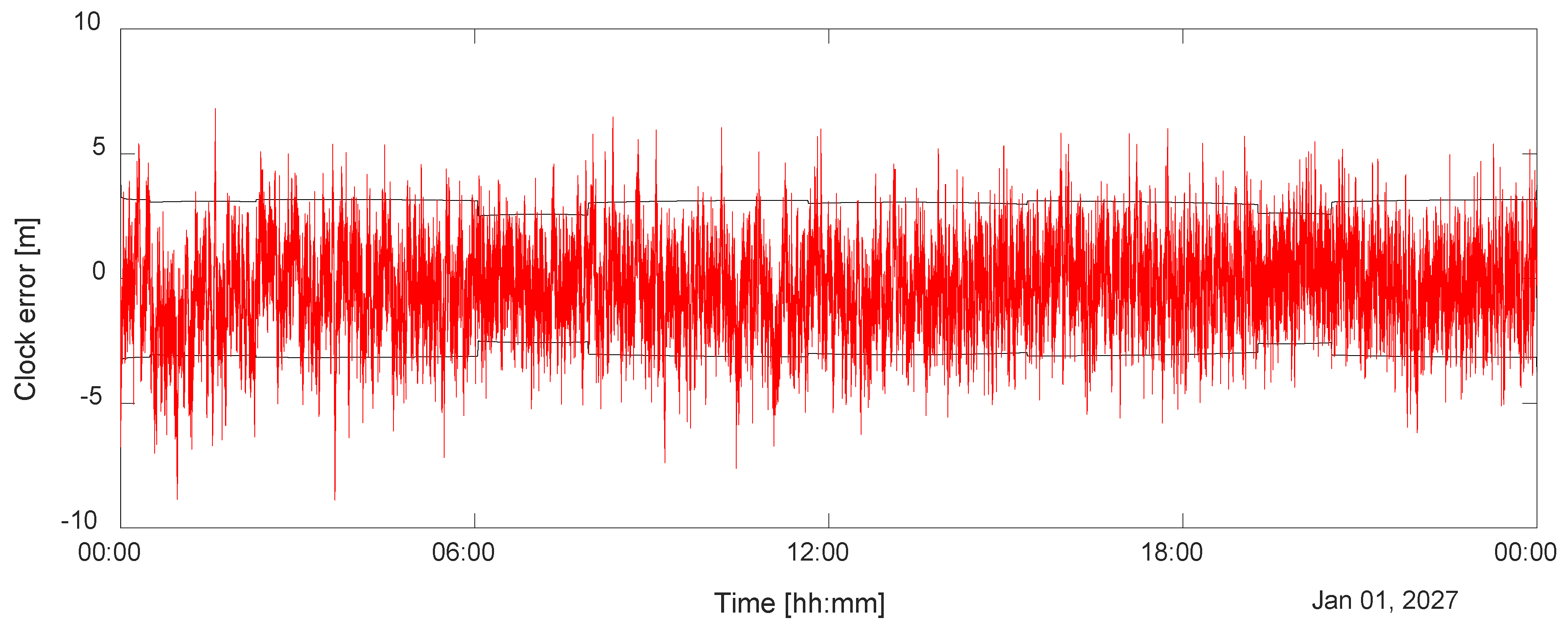
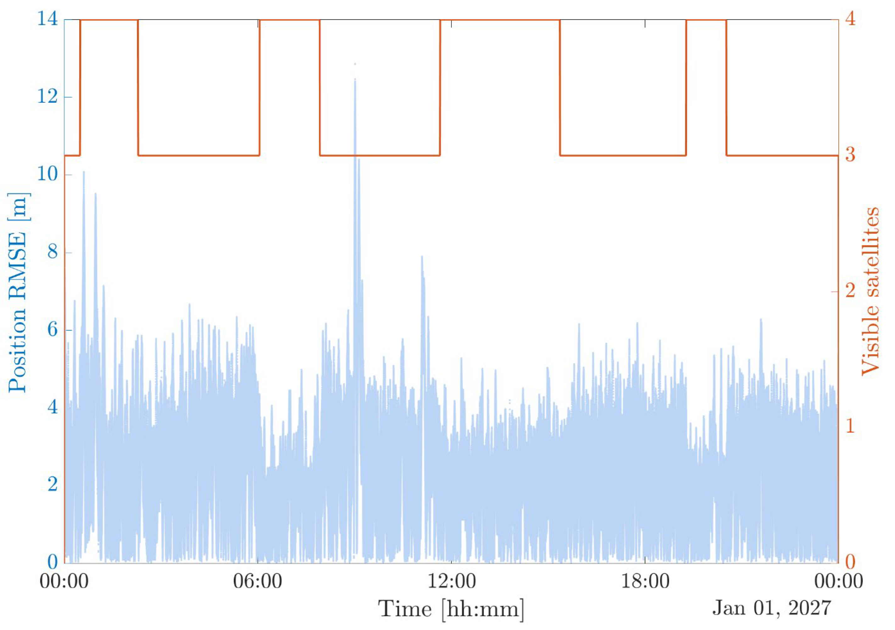
In this first scenario, the rover can only rely on satellite navigation. Unfortunately, the recurrent periods of poor visibility (i.e., only three satellites available) do not allow for accurate navigation. As it is possible to see from Figure 8, the unknown trajectory of the rover does not permit an accurate prediction in the time in which three satellites are visible, and the error periodically diverges. Similar behavior, as expected, can be detected in the clock error (Figure 9).

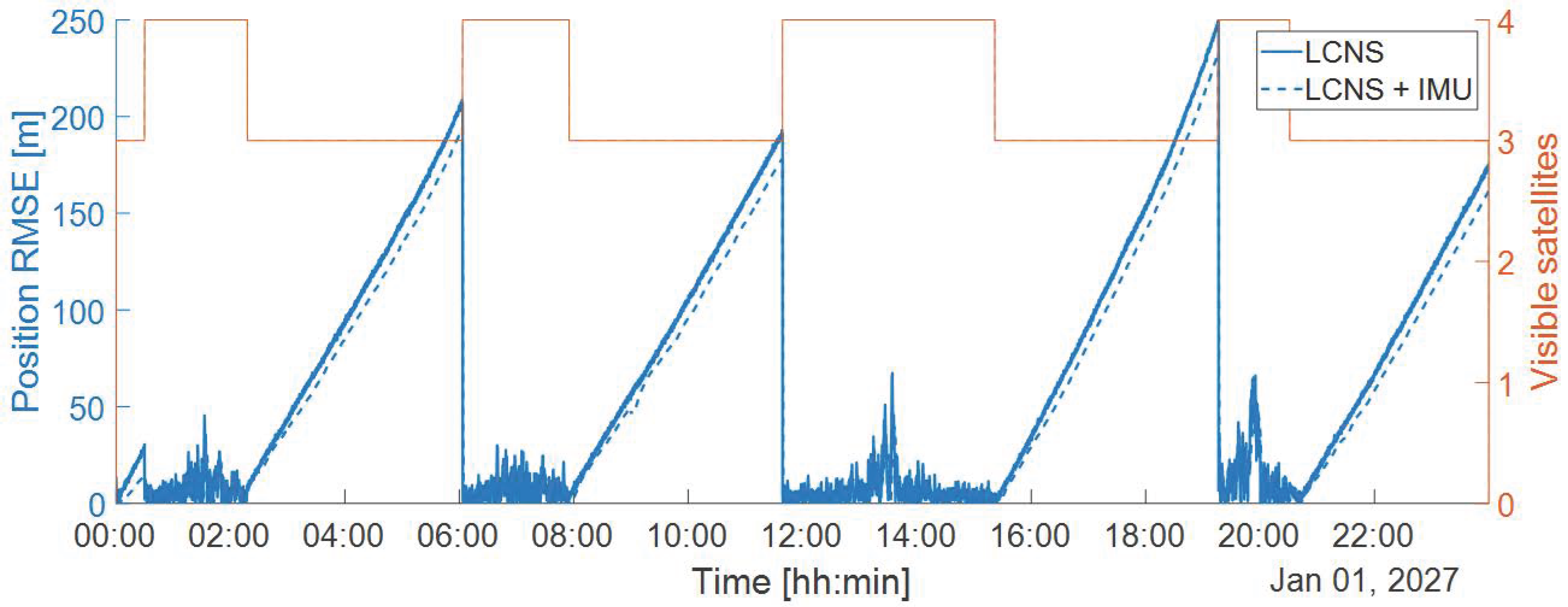
6.2. LCNS + IMU

In this second simulation, the IMU is used together with satellite navigation. The position root mean square error, plotted in Figure 10, shows limited improvements. In fact, the IMU contribution is strongly dependent on the last estimated position and velocity, which is, however, poorly accurate due to the limited visibility of the ELFO satellites.

In this condition, the statistical analysis of the error, reported in

Table 8. Error statistics for the case LCNS + IMU.

Error Type (95th Percentile)	Value
Position	173.49 m
Horizontal position	44.17 m
Velocity	0.05550 m/s
Horizontal velocity	0.02228 m/s
Time	432.1 ns

, suggests that accurate navigation of the rover is not possible. Here and in the following, the 95th percentile, i.e., the value below which 95% of the data points falls, is used as a metric for the analysis of navigation performance.

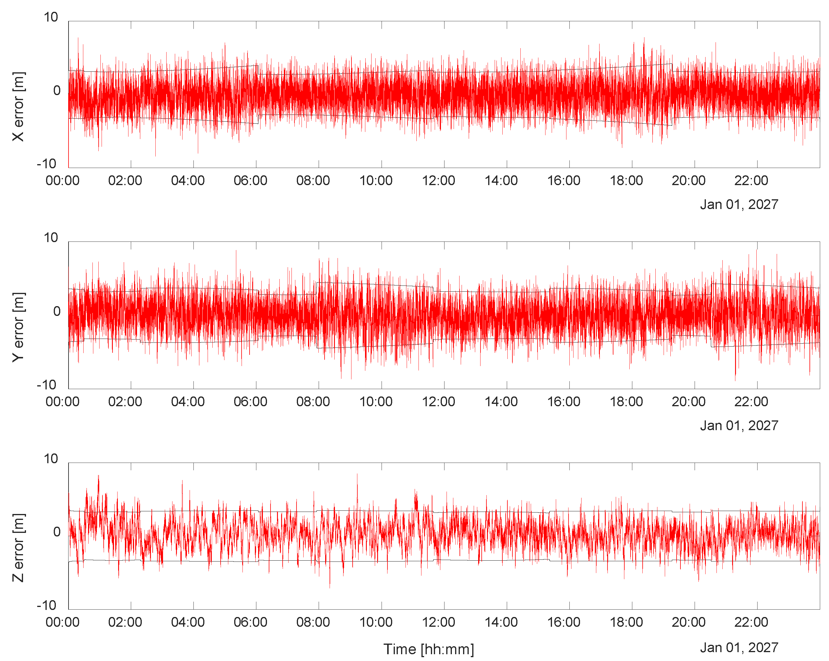
6.3. LCNS + DEM

A remarkable improvement can be achieved if a DEM is available. This additional source of information is comparable (in terms of effects on the estimation accuracy) with a virtual fifth ELFO satellite. In fact, observing Figure 11 and Figure 12 for the error on the coordinates and the time, respectively, the performance in this case is far less affected by the times in which only three satellites are visible. The statistics summary in

Table 9. Error statistics for the case LCNS + DEM.

Error Type (95th Percentile)	Value
Position	5.45 m
Horizontal position	4.79 m
Velocity	0.0815 m/s
Horizontal velocity	0.0748 m/s
Time	11.74 ns

shows that in this case, a navigation with meter-level accuracy is possible, with nearly two orders of magnitude improvement on the position with respect to the case in which the DEM is not used. Quite interestingly, the lack of an IMU produces a worsening of the velocity estimates.

6.4. LCNS + DEM + IMU

As easily predictable, the best performance can be achieved when implementing a navigation filter that uses information from LCNS, DEM, and IMU (see Figure 13). In particular, the horizontal position error decreases by about 40%, while the horizontal velocity drops by a remarkable 78% (see the statistics in

Table 10. Error statistics for the case LCNS + DEM + IMU.

Error Type (95th Percentile)	Value
Position	4.05 m
Horizontal position	2.84 m
Velocity	0.02795 m/s
Horizontal velocity	0.01686 m/s
Time	11.74 ns

compared with the ones in Table 9).

7. Simulation Results: Monte Carlo Run

A single run could be considered not sufficient to assess the performance in a reliable way. Therefore, a Monte Carlo approach is implemented, running the same simulation of paragraph 6.4 (including LCNS, DEM and IMU) 100 times using sensors measurements that differ because of their random characteristics.

Figure 14, Figure 15 and Figure 16 reports the error plots of the 100 runs relevant to the position, the velocity, and the clock, respectively. The statistics can be computed by assembling all the error time histories in a single vector and taking the statistics, or by taking the statistics of each run and then taking the average of the 100 statistics. The results are qualitatively the same with both approaches; the first mode has been used in this analysis, and the results can be found in

Table 11. Error statistics for the LCNS + DEM + IMU: Monte Carlo run case.

Error Type (95th Percentile)	Value
Position	4.05 m
Horizontal position	2.7 m
Velocity	0.02812 m/s
Horizontal velocity	0.01622 m/s
Time	11.71 ns

. At the qualitative level, they confirm all the findings that have been reported for the single run in paragraph 6.4.

8. Simulation Results: Convergence Analysis

In all previous analyses, the initial condition was perfectly known. The capability of the navigation algorithm to converge, and the convergence time must be now analyzed. To keep the study simple, the initial error $e_0$ on the estimate is scaled with a single common parameter k:

$$e_0=[k, k, k, 0.01k, 0.01k, 0.01k, k, 0.01k]$$

The parameter k varies from 100 to 20,000, meaning a 20 km error in all directions. Further increases in the parameter are not possible because of the limited spatial extension of DEM used. The convergence of the filter is verified in all considered cases. If a value of error of 10 m is arbitrarily fixed as the threshold for assessing the convergence, it is possible to see from Figure 17 that even in the most uncertain initialization, about 35 min is sufficient to acquire an accurate position.

9. Conclusions

This study has analyzed the navigation performance of a lunar rover utilizing the Lunar Communication and Navigation Services (LCNS) in combination with additional sensors, including an Inertial Measurement Unit (IMU) and a Digital Elevation Model (DEM). The results demonstrate that standalone LCNS navigation suffers from degraded accuracy due to frequent periods of limited satellite visibility. However, integrating supplementary sensors significantly improves positioning performance.

Specifically, the inclusion of a DEM is the key factor, enhancing horizontal positioning accuracy and effectively acting as an additional virtual satellite. The integration of an IMU further contributes to refining velocity estimation, though its benefits are most evident when combined with the DEM. The full sensor suite (LCNS + DEM + IMU) of course achieves the best results, but a reasonable accuracy can be obtained when even giving up the IMU.

A Monte Carlo analysis confirms the robustness of these findings, demonstrating that the proposed sensor fusion approach yields reliable and repeatable improvements in navigation accuracy. Additionally, convergence analysis indicates that even with large initial uncertainties, the filter can provide an accurate position estimate within approximately 35 min. These results highlight the importance of multi-sensor integration for lunar surface navigation, providing a practical pathway for achieving high-accuracy localization in future lunar exploration missions.