Enhancing Model Generalizability in Aircraft Carbon Brake Wear Prediction: A Comparative Study and Transfer Learning Approach

Abstract

Predictive maintenance in commercial aviation demands highly reliable and robust models, particularly for critical components like carbon brakes. This paper addresses two primary concerns in modeling carbon brake wear for distinct aircraft variants: (1) the choice between developing specialized models for individual aircraft types versus a unified, general model, and (2) the potential of transfer learning (TL) to boost model performance across diverse domains (e.g., aircraft types). We evaluate the trade-offs between predictive performance and computational efficiency by comparing specialized models tailored to specific aircraft types with a generalized model designed to predict continuous wear values across multiple aircraft types. Additionally, we explore the efficacy of TL in leveraging existing domain knowledge to enhance predictions in new, related contexts. Our findings demonstrate that a well-tuned generalized model supported by TL offers a viable approach to reducing model complexity and computational demands while maintaining robust and reliable predictive performance. The implications of this research extend beyond aviation, suggesting broader applications in component predictive maintenance where data-driven insights are crucial for operational efficiency and safety.

1. Introduction

The relentless quest for enhancing safety and operational efficiency in commercial aviation has accelerated the development and application of advanced predictive maintenance techniques [1,2]. Central to this effort is the focus on braking systems—components of paramount importance for ensuring safe takeoffs and landings. The advent of sophisticated sensor technology has created a data-rich environment ideally suited for applying machine learning (ML) in the predictive maintenance of these critical systems [3]. More specifically, the design of electrically actuated brakes on the main landing gear of a certain widebody aircraft integrates advanced wear-pin sensors on each of its eight brakes. These sensors provide a stream of data that offers semi-instantaneous insights into the condition of the brake components, including the remaining thickness of the carbon brake pads. This connectivity and the wealth of available data present an opportunity for the development of a digital twin (DT)—a virtual model that mirrors the physical attributes and behaviors of the carbon brakes [4,5].

The concept of a DT has emerged as a transformative tool, serving as a ‘representation of a connected physical asset’, enabled by continuous data/information exchange between the DT and its physical counterpart [6,7,8,9,10]. Of particular interest in this paper is the generalizability of DTs, that is, their predictive capability to be accurate, adaptable, and resilient. The objective is to create a model that mirrors a real-world system precisely such that it can accommodate and predict the consequences of unforeseen changes, which is indispensable for several reasons. First, real-world systems are dynamic entities; they may undergo operational modifications, such as an aircraft operating in a new environment. Such changes would not throw off balance a model that generalizes well. Instead, it adapts, thereby remaining reliable and accurate in its predictions [5]. Second, there is substantial value across variations, a concept also integral to generalizability. For instance, for an aircraft model that comprises diverse configurations, a generalized model would not be limited to the variant it was initially trained on, signifying its robustness across a spectrum of similar yet distinct systems.

In the context of this research, it is understood that each tail number is subject to operational and environmental variations due to the nature of the routes it flies, the airports it takes off from and lands at, the crew operating the aircraft, etc. As a result, we are interested in developing a predictive DT that generalizes well across different aircraft types, i.e., whose brake wear predictive capabilities are robust and reliable enough to be applied consistently across all variants within the same fleet.

One key challenge to address in developing DTs that generalize well across different variants is overfitting—a common pitfall where a model, tuned too closely to the training data, loses its ability to predict accurately on new, unseen data [11]. A model’s ability to generalize well acts as a safeguard against overfitting—it learns from the training data without being hindered by noise and outliers, ensuring reliable performance when faced with new conditions [12]. Mitigating overfitting is critical to ensure that the DT remains a reliable tool for maintenance and operational planning.

Another important consideration is the cost and time efficiency of developing a generalizable digital twin (DT) model. Such a model can significantly reduce resource requirements by being applicable to various operational scenarios and systems, thereby eliminating the need to retrain it from scratch for each new route or aircraft variant. This capability enables rapid deployment, which is especially critical in fast-paced industrial environments [13]. Within this landscape, transfer learning (TL) emerges as a robust solution for improving model adaptability. It allows knowledge gained from one task to be leveraged for different yet related tasks [14,15,16,17,18].

Xu et al. highlight the practical relevance of TL—particularly deep domain adaptation—for addressing data scarcity, and categorize TL methods into fine-tuning, adversarial adaptation, and sample-reconstruction approaches [14]. Tan et al. provide a foundational survey that defines deep TL and classifies it into four distinct types, emphasizing its utility in reducing data requirements and training time, particularly in non-independent and identically distributed (non-i.i.d.) domains [15]. Weiss et al. [16] offer a comprehensive review that underscores TL’s value when training and test data distributions differ, citing successful applications in domains such as text sentiment analysis, activity classification, and image recognition. Kouw and Loog provide a theoretical grounding in domain adaptation and TL, introducing strategies for managing dataset shifts—such as covariate, prior, and concept shifts—between source and target domains [17]. Finally, Pan and Yang present a seminal survey that formalizes the taxonomy of TL and reinforces its importance in reducing labeling costs by enabling model adaptation across domains with differing feature spaces or distributions [18].

By adopting a model pre-trained on a large and representative dataset—such as one based on a specific aircraft type—and fine-tuning it on a smaller dataset representing another variant, TL offers a powerful strategy for achieving high model generalizability, reliability, and efficiency [15,16,17,18]. This is especially relevant in predictive maintenance for complex systems like aircraft brakes, where training time and data availability are often constrained.

This paper is structured as follows. Section 2 reviews the relevant literature on brake wear prediction, identifying existing gaps in the field and highlighting the contributions of this study. Section 3 provides an overview of the datasets utilized, including full-flight data from an airline’s widebody aircraft operations, alongside weather information and airport characteristics sourced from FlightAware^® (Houston, TX, USA). Section 4 outlines the methodologies for two key experiments designed to evaluate and enhance model generalizability. The first experiment assesses model performance across different domains, represented by data segments from distinct variants of a specific widebody aircraft. The second experiment explores the potential of TL to improve model adaptability, evaluating its effectiveness in transferring knowledge from models trained on one or more aircraft variants to others. Section 5 describes the implementation of these experiments, and Section 6 provides an analysis of the results. Finally, Section 7 summarizes the findings and suggests directions for future research.

2. Literature Review

This section provides an analysis of existing contributions in the field of brake wear prediction, highlighting substantial gaps in research and underscoring the significance of this study.

2.1. Need for Operational Variability and Model Generalizability in Brake Wear Prognostics

Effectively predicting brake wear is a challenge that is common to both the aviation and automotive industries, with various methodologies being proposed and evaluated for their efficacy. A significant contribution to this field is the work by Oikonomou et al., who investigate the potential of data-driven, probabilistic methods to forecast the remaining useful life (RUL) of aircraft brakes using historical data from an airline’s widebody fleet [19]. In their study, three distinct approaches are assessed: a non-homogeneous hidden semi-Markov model (NHHSMM), artificial neural network (ANN) with bootstrapping, and Bayesian linear regression (BLR). The research simplifies the input variables to only the sensor value of the brake pad’s thickness and the count of flights conducted by the aircraft, with the target output being the projected RUL in terms of remaining flights. Notably, the study strategically excludes outliers—the brake degradation profiles that diverge significantly from the average lifespan—reserving them solely for testing the models. The authors employ evaluation metrics that focus on the latter 75% of the brake’s lifespan while disregarding the initial 25% [19]. This approach to performance evaluation can potentially skew the perception of the model’s accuracy, as it fails to consider the entire operational life of the brake. For instance, the NHHSMM model exhibits notable deficiencies in capturing real-world performance during the early stages of brake usage. Conversely, the bootstrapped ANN emerges as the most competent model, yet it too falls short in reliably forecasting the RUL for anomalies—those instances purposely set aside for model testing [19]. This model’s failure to adapt to deviations in brake lifespan, both shorter and longer than expected, highlights a critical gap in predictive modeling: the model’s ability to generalize, especially when dealing with brake conditions outside the typical operational range. This underscores the necessity for a comprehensive model assessment over the entire lifespan of the brake, thus ensuring both reliability and robustness to accommodate the full spectrum of operational scenarios. This research aims to expand the literature by addressing these gaps and exploring the implications of a generalizable model within the context of DTs in aircraft maintenance.

In another effort, Choudhuri et al. sought to alleviate the financial and temporal burdens that automotive companies face when testing various brake pad material combinations on dynamometers to identify optimal constituents. They proposed an innovative solution utilizing ANNs to predict brake and disc wear, demonstrating the potential to forecast wear for new brake pad designs. Nevertheless, the model’s effectiveness remains constrained by its specificity to certain driving styles and route configurations [20]. The study does not extend to investigating how variations in these factors could influence the wear on brakes or disks, leaving a gap in understanding the broader applicability of the ANN’s predictions. Additionally, the training data are synthesized from a lab setup under different braking regimes, which may not fully encapsulate the real-world operations of a vehicle. Initially, the ANN yielded an accuracy of approximately 60%; however, the wear prediction error was disproportionately higher at elevated speeds than at lower speeds. In response, Choudhuri et al. did not opt for model optimization or retraining with a more extensive dataset to enhance the ANN’s generalizability. Instead, they developed two distinct ANNs: one for low-speed wear predictions and another for high-speed scenarios. This bifurcation of models led to a notable improvement in accuracy, reaching around 85% [20]. Yet, maintaining multiple ANNs introduces a host of complexities, such as escalating the models’ maintenance efforts, adding to the training time and computational costs, and increasing the storage requirements. Their research highlights the trade-off between predictive performance and operational efficiency, specifically the practical challenges of deploying and maintaining multiple models, such as increased time, costs, and complexity. It also prompts a significant question for further research: Can an overarching model be developed to reliably forecast wear across diverse conditions while maintaining computational and operational efficiency? The current study aims to delve into this question, exploring the possibilities of TL to translate into more generalizable models for the context at hand.

In another effort, Harish et al. directed their research toward understanding the influences of vehicle dynamics and road attributes on brake system forces [21]. An accelerometer gathered vibration data from simulated fault states and normal functioning using a brake setup and a static road simulator. Despite classifying driving scenarios across low, medium, and high speeds, ML models were solely developed using low-speed conditions, a limitation that Harish et al. acknowledged. The LogitBoost Meta, which combines logistic regression with the boosting power of AdaBoost, emerged as the most accurate classifier within this constrained environment [21]. The research also underscores the necessity to experiment across a broader spectrum of braking dynamics and operational conditions, resonating with the overarching theme of generalizability.

Küfner et al. advocate for solutions that optimize the use of ML in decentralized computing systems [22]. Using current signatures of production facilities, their study harnesses recurrent neural networks (RNNs) to classify varying degrees of wear and determine operational states within a manufacturing setup. The methodology was underpinned by an experimental brake wear simulation, which, due to the consistent conditions of the setup, presumed linear wear behavior. This research stands out for its implementation of two types of RNNs: long short-term memory (LSTM) and the gated recurrent unit (GRU), with the latter achieving over 95% accuracy, especially in predicting critical wear stages. These algorithms were integrated within an embedded system for real-time wear detection at the machine’s edge, albeit constrained by the available hardware resources. This limitation affected the model’s capacity for optimization, such as expanding the number of GRUs or sequence analysis windows. Furthermore, the model faced limitations in its training data scope, which restricted its ability to recognize conditions beyond its training. The study did not explore the model’s transferability to different manufacturing contexts, which remains an area for future investigation [22]. This paper highlights the balance between model sophistication and computational feasibility, an equilibrium that this current research aims to investigate through the lens of generalizable and transferable predictive models.

In the realm of component health management, Magargle et al. have critically examined current methodologies, which are predominantly data science-driven with minimal integration of physical principles, finding them confined mainly to diagnostic applications [23]. In their research, a physics-based approach was employed for monitoring heat and conducting predictive maintenance of automotive brakes. The simulated DT, exposed to multiple failure scenarios, produced abnormal pad wear and sensor signals, using finite element analysis (FEA) and the Archard Wear Model. The simulations involved different pressure and speed combinations to construct a wear response surface. The results covered a spectrum of scenarios, including standard and faulty antilock braking system (ABS) operations and sensor functionalities. While Magargle et al. recognized the necessity for more detailed physical models to cover additional operating conditions, it is essential to note that their high-fidelity model is invaluable for identifying sensor patterns in fault conditions conducive to training ML algorithms [23]. Still, it lacks the operational variability found in real-world data.

2.2. Observations from Literature and Research Contributions

The existing body of literature on brake wear prediction, spanning both aerospace and automotive sectors, points to a common trend: predictive models are often tailored to specific operational conditions or vehicle types, thus limiting their broader applicability [19,20,21,22,23]. For instance, Oikonomou et al.’s models, derived from homogeneous fleet data, do not accommodate operational variability and treat outlier data as a separate entity reserved for testing purposes only [19]. This siloed approach is mirrored in Choudhuri et al.’s work, where distinct neural networks were constructed for different speed regimes to address discrepancies in predictive performance, thus multiplying the effort and cost associated with model maintenance and computational resources. Their models’ capabilities were also confined to specific driving styles and routes, indicating a narrow generalizability scope [20]. Similarly, Harish et al. limited their fault condition simulations to city driving scenarios without testing under varied conditions, while Küfner et al. and Magargle et al. relied on simulated data under constant conditions, neglecting the impact of environmental and operational variations on model performance [21,22,23]. These studies collectively underscore a significant gap in the literature: the pressing need for improved model generalizability to account for variability within a specific sector, such as across vehicle variants, operating conditions, and environmental contexts.

In this context, the contributions of this research are two-fold:

• First, a comprehensive assessment of the need for model generalizability is provided by comparing a generalized, fleet-based model to specialized models on each data segment (e.g., aircraft variant). This evaluation extends beyond the traditional, more constrained datasets to include variations in aircraft-specific parameters (such as weight and speed), operational conditions (such as flight duration and turnaround time), environmental factors (such as static air temperature and humidity), and airport characteristics (such as elevation and runway length). Doing so aims to demonstrate the importance of generalizability in predictive modeling for aircraft maintenance.
• Next, the efficacy of TL in enhancing model generalizability is assessed by developing models that predict carbon brake pad wear for specific aircraft variants and then applying TL to adapt these models for predicting wear on other variants. This approach evaluates TL’s ability to leverage knowledge from pre-trained models on one or more aircraft types to improve predictions on new, related variants, enabling the creation of adaptable and robust models that perform well across varying operational and environmental conditions. The findings aim to reduce the need for independently specialized models, streamlining the predictive process and reducing its complexity and resource requirements.

Beyond these primary contributions, the paper also offers insights into the computational cost–benefit trade-offs of different modeling approaches. It lays the groundwork for future research in applying ML to predictive maintenance, challenging the existing paradigm by advocating for more versatile and computationally efficient modeling strategies that ensure robust predictive performance and reliability.

3. Available Data

This section outlines the dataset used in this research, which comprises specific parameters from actual full-flight operations provided by an airline, along with environmental conditions and airport characteristics sourced from FlightAware^®.

3.1. Continuous Parameter Logging (CPL) Data

CPL data constitutes a systematic compilation of operational parameters measured throughout the flight lifecycle, from engine ignition to cessation. Recorded in real-time at a frequency of one hertz (i.e., one recording per second for each signal) by onboard systems and sensors, this dataset offers an exhaustive log that encompasses the aircraft’s performance metrics (such as airspeed and altitude), engine parameters (such as temperature and fuel consumption), control surface statuses, cockpit commands, and pertinent environmental data such as outside air temperature. These logs fulfill multiple objectives, including aircraft health monitoring, performance optimization, regulatory compliance, and safety enhancement by preemptively identifying potential issues [24,25,26]. They are also indispensable for post-flight evaluations, maintenance schedules, and incident inquiries [27,28]. The data, stored in the quick access recorder (QAR) or transmitted to ground systems in real-time, are essential for predictive maintenance capabilities and operational enhancements in aviation [29,30].

The CPL data used in this research are sourced from the real-world operations of an airline that operates a widebody aircraft fleet comprising three distinct variants: Variant 1, the smallest; Variant 2, the medium-sized variant; and Variant 3, the largest. Due to intellectual property and confidentiality agreements, the specific airline and aircraft types are not disclosed. This dataset contains over 800 parameters and has been available since July 2017. Figure 1 illustrates sample CPL signals from a single flight, including cabin altitude, static air temperature, ground speed, gross weight, flight phase, and an on-ground indication. The airline’s widebody fleet includes 71 aircraft, distributed as follows: 36 tails of Variant 1, 32 tails of Variant 2, and 3 tails of Variant 3. This diverse fleet composition provides a robust basis for analyzing model generalizability across aircraft of varying sizes and operational characteristics.

3.2. FlightAware^® Data

FlightAware^®, a digital aviation company, provides real-time and historical data, including detailed weather information and airport characteristics [31].

3.2.1. Weather Data

A Meteorological Aerodrome Report (METAR) offers a current snapshot of weather conditions at an airport. It is typically updated hourly, though additional reports may be issued during significant weather changes. FlightAware^®’s weather data are sourced from METARs, an example of which is presented in Figure 2 below [32]. These data, available since April 2021, include essential parameters such as temperature, wind speed and direction, visibility, cloud cover, atmospheric pressure, and other notable weather phenomena.

3.2.2. Airport Data

FlightAware^® also provides airport-specific data that include aggregated runway information, such as average, minimum, and maximum runway lengths, along with geographical details like latitude, longitude, and elevation. However, these data are generalized, with only a single row of information available for each airport. Consequently, they do not differentiate between individual runways within the same airport, potentially limiting the precision of analyses that require runway-specific details. Despite this limitation, the aggregated data remain a valuable resource for understanding an airport’s overall size and layout, which can significantly impact aircraft operations. For example, runway lengths influence the required braking force and, consequently, brake pad wear, while an airport’s elevation and location shape the environmental conditions affecting aircraft and braking performance.

4. Methodology

The literature review in Section 2 reveals a notable gap in the generalizability of models, which often fail to perform uniformly across different operations, environments, or vehicle types. This section outlines the methodologies for two experiments aimed at evaluating and enhancing generalizability. The first focuses on assessing model generalizability across different domains, represented by data segments corresponding to the different variants of a particular widebody aircraft. This experiment underscores the necessity of ensuring model robustness across different aircraft types. The second experiment then investigates the potential of TL to enhance model generalizability across these diverse data domains, evaluating its effectiveness in adapting models trained on one or more aircraft variants to perform well on others.

4.1. Experiment 1: Assessing Model Generalizability

The pursuit of model generalizability within predictive analytics for aircraft operations has become a subject of particular importance [33,34,35]. When examining the carbon brake degradation profiles, discrepancies in wear rates emerge across aircraft types. The left plot in Figure 3 shows cumulative brake degradation over time for each brake, expressed as a percentage from the initial wear pin value at installation (0%), with degradation increasing by flight number. Larger variants (Variants 2 and 3) display steeper degradation trends compared to Variant 1. The right plot presents a histogram of per-flight degradation—defined as the wear pin value difference per flight (%)—which further confirms the higher wear rates observed in Variants 2 and 3. One approach to address this issue involves segmenting the data into specific groups, such as by aircraft type, and training distinct models for each data segment. While this specialization could enhance the predictive performance for each subset, it introduces significant complexities in model management and maintenance, such as updating multiple models, as well as increased computational demands due to longer training durations and higher storage requirements to accommodate the models.

The central research question is whether it is necessary to create individualized models tailored to specific aircraft types, or if a single, generalized model can be developed to effectively span the entire fleet. The implications for the predictive performance and reliability of these models are significant. Given the similar underlying wear mechanisms across all variants, a generalized model may provide broader applicability while maintaining sufficient predictive capability. In contrast, specialized models may be more finely tuned to their respective variant’s data, potentially improving performance for individual subsets. However, this comes at the cost of increased complexity in model management and maintenance, as well as greater resource demands.

A methodological framework, summarized in Figure 4, is designed to meticulously evaluate the trade-offs in model specialization versus generalization and determine the optimal approach for predicting carbon brake wear across different aircraft variants.

The methodology for Experiment 1 involves eight key steps, beginning with engineering per-flight features from raw full-flight data from aircraft operations and integrating them with relevant weather information and airport characteristics derived from FlightAware^®. Next, the data are preprocessed, which includes cleaning, transforming, and normalizing them in preparation for subsequent modeling. Following this, the data are split into training and testing sets, stratified by aircraft tail numbers for each variant. A generalized model is then trained on the entire fleet’s data using a deep neural network (DNN). Additionally, specialized models are trained separately for each aircraft type. To assess performance, the generalized model is tested on each aircraft variant separately, while specialized models are evaluated against their corresponding variant’s test data. Next, RMSE and additional metrics are used to determine differences in performance between the fleet-based and specialized models. Finally, the results are analyzed to conclude whether individual models for specific aircraft classes are necessary. The next section of this paper will provide a detailed explanation of each of these steps.

4.2. Experiment 2: Enhancing Model Generalizability Through TL

Building on the foundational experiment conducted to assess model generalizability in the predictive analytics of aircraft brake wear, the potential of TL to improve the model’s capability to generalize across different domains (i.e., data segments) is of great interest. As mentioned, the core premise of TL is to leverage knowledge acquired while addressing one problem and then apply it to different but related tasks [14,15,16,17,18]. This approach can be significant when developing a singular predictive model that performs well across various aircraft types, even when data availability for each type varies significantly. In this context, TL can be particularly effective due to the underlying similarities in braking system design and the physical mechanisms that govern wear across aircraft variants. While all three variants are equipped with the same electrically actuated braking system, the observed brake wear behavior—such as the rate and steepness of degradation—can vary due to factors like aircraft mass and operational usage. For instance, Variant 3, being the largest, tends to exhibit steeper degradation profiles compared to Variant 1, as illustrated in Figure 3. Nevertheless, the core physics driving brake wear remain consistent across variants, making TL a suitable approach for transferring learned patterns from data-rich variants to those with limited data representation.

Two primary TL approaches, weight initialization and feature extraction, are considered as they are among the most commonly used and effective strategies in leveraging knowledge from a related domain to address practical challenges, such as limited data availability for specific tasks [36]:

• Weight initialization: This approach uses the weights from layers of a model trained on a related, data-rich problem as the starting point for training another model on the new task of interest. The model can swiftly adjust to the new task by leveraging pre-trained weights, utilizing the commonalities between the problems to accelerate learning and improve performance [36]. This approach allows the model to start with a well-informed set of parameters and is particularly useful when there is an imbalance in the size of datasets available for different aircraft variants, as it reduces the need for extensive training on smaller datasets. For instance, a model pre-trained on Variant 1 data with an abundance of labeled samples can have all of its weights adjusted to learn the specifics of the Variant 3 problem despite the smaller dataset size for the latter. In this case, none of the pre-trained model’s layers are frozen.
• Feature extraction: In this method, the neural network weights trained on the initial problem are kept fixed, and only the layers added after the reused ones are trained further to interpret the output for the new problem. The shared foundational features across domains are typically captured in the lower layers of a neural network. By freezing these layers, the model preserves the learned representations and focuses on learning patterns in the new data [36]. Since the operational conditions and degradation trends across aircraft variants share core similarities, the extracted features from one or more variants can serve as a robust foundation. This reduces the complexity of retraining the entire model and ensures an efficient use of limited data for specific variants. For instance, by keeping the hidden layers trained on data from Variants 1 and 2 fixed, the model can only learn the output layer weights for Variant 3 data, ensuring that the core features extracted from the initial dataset are utilized effectively.

Weight initialization provides a starting point for training on the new task, while feature extraction emphasizes efficiency and robustness in preserving foundational knowledge. Both techniques were incorporated in Experiment 2 to refine the predictive models for aircraft brake wear by harnessing and repurposing knowledge from one domain (e.g., a certain aircraft variant) for use in another. This tailored approach is detailed in Figure 5.

5. Implementation

This section details the implementation of each step for Experiment 1, which assesses model generalizability across different aircraft variants, and Experiment 2, which explores the potential of TL to enhance generalizability across these diverse data domains.

5.1. Experiment 1: Assessing Model Generalizability

This experiment assesses model generalizability across different aircraft variants by comparing the performance of a generalized fleet-based model to that of individual specialized models tailored for each variant. The experimental framework is depicted in Figure 6 below and each of its steps is detailed next.

5.1.1. Engineer Features and Fuse Data

As mentioned, the comprehensive CPL dataset originates from an airline’s fleet of 71 widebody aircraft, divided into 36 units of a smaller-sized variant, 32 units of a medium-sized variant, and 3 units of a larger-sized variant. This dataset comprises hundreds of thousands of full-flight files, available since July 2017, providing a rich foundation for analysis. However, with over 800 recorded parameters, it is crucial to filter and prioritize those most relevant to brake wear, streamlining the analysis to focus on the most impactful factors. To address the challenge of the dataset’s high-resolution, per-second data—potentially overwhelming for specific ML models—a strategy is adopted to generate per-flight features for each aircraft’s eight brakes.

Table 1. Sample per-flight features generated from CPL data *.

Operational and Utilization Metrics	Aircraft, Technical, and Environmental Metrics	Wheel and Brake Metrics		Pilot Inputs and Engine Metrics
Airport ICAO Codes	Aircraft ID/Tail Number	Brake Position	Mean Wheel Speed *	Autobrake Setting Indicator
Flight Start/End Timestamps	Aircraft Class	Wear Pin Value	Wheel Energy *	Thrust Reverser Usage Indicator
Tail Flight Number	Mean Ground Speed *	Brake Command (CMD) Fraction *	Mean Brake CMD *	Mean Captain or First Officer Pedal Force *
Flight Duration	Deceleration *	# of Brake Applications *	Mean and Max Brake Temperature Monitoring System (BTMS) Brake Temperature *	Mean Engine N1 Left/Right *
Tail Flight Count Per Day	Aircraft Weight *	Mean Autobrake Master CMD *
Rolling Average Flights/Day (Window: 100 Flights)	Mean Kinetic Energy *	Mean Tire Pressure *
Time Between Flights	Mean Cabin Altitude *	Wheel Wear *
Time Duration *	Static Air Temperature *	Mean Electronic Brake Actuator Force *
Tail Flight # of the Day		Parking Brake Sum *

* Features marked with an asterisk (*) are calculated separately for each of the three flight phases: taxi-out, landing, and taxi-in.

outlines examples of the specific features generated, offering a streamlined yet detailed perspective on the braking system’s performance.

The features were selected based on their relevance to brake wear, encompassing aircraft-specific parameters (e.g., weight and speed), operational factors (e.g., flight duration), and environmental conditions (e.g., static air temperature). To condense the 1 Hz raw CPL data into meaningful per-flight features, the data were aggregated using metrics such as maximum or average values for each parameter. A process was developed to interrogate and extract the specified features of interest from individual flight files. This approach was then scaled across the entire dataset using PySpark 3.4.1, enabling an efficient parallel analysis of the comprehensive full-flight data. This feature engineering approach also ensures a holistic understanding of braking system performance across different flight phases where brake usage peaks:

• Taxi out (including power on, engine start, taxi out, and takeoff roll)
• Landing (covering flare and rollout)
• Taxi in (encompassing taxi in, engine shutdown, and maintenance).

For each phase, certain features are calculated to capture the operational conditions affecting the brakes. For instance, the mean cabin altitude during each flight phase is included to provide additional context.

The refined dataset offers detailed insights into the factors contributing to brake wear by analyzing a mix of pilot inputs and brake system interactions (e.g., pilot pedal force and autobrake setting), aircraft specifics (e.g., tail number and aircraft type), and operational conditions (e.g., turnaround time and daily flight count). These comprehensive data are the foundation for deploying ML methods to predict carbon brake wear, thereby aiding in developing more knowledgeable maintenance strategies and improving safety measures. Enhancing the dataset with weather and airport data from FlightAware^® provides a more comprehensive understanding of the environmental and operational conditions influencing aircraft and braking system performance at destination airports.

FlightAware^® weather data, derived from METARs, includes metrics such as cloud altitude, pressure, air temperature, dew point, relative humidity, and visibility, as well as wind speed, wind direction, and gusts [32]. As these data have been available since April 2021, the dataset used in this research spans from April 2021 to October 2023, encompassing over 90,000 full-flight files. These weather data are integrated with CPL data by aligning them with the destination airport and the arrival time (within one hour of arrival), providing a more detailed view of the environmental conditions impacting each flight. In addition to weather information, FlightAware^® also provides general airport characteristics, including geographic details (latitude, longitude, and elevation) and runway lengths (minimum, maximum, and average). These elements further enhance the dataset, enabling more robust brake wear prediction modeling.

Note that the effectiveness of a generalized model depends significantly on its ability to capture relationships across the fleet’s operational diversity. The choice of aircraft specifics, environmental conditions, and operational factors ensures a model can learn patterns applicable across multiple aircraft variants. If the features fail to represent critical aspects of brake wear, the model might exhibit subpar performance, especially on less-represented variants. The feature engineering process also impacts the success of TL in the subsequent experiment by determining whether the shared layers encode broadly applicable knowledge. For instance, including universally relevant features like brake temperatures allows the pre-trained model to adapt effectively. Conversely, overly specific features (e.g., tail number) might restrict the model’s ability to generalize, requiring extensive fine-tuning during TL.

5.1.2. Preprocess Data

The data preprocessing phase refines the dataset for precise and practical training of supervised ML algorithms. The process involves several meticulous steps to ensure the dataset’s readiness for model development. The steps undertaken are as follows.

• Feature dropping based on correlation: Initially, redundant features presenting a high risk of multicollinearity are identified and discarded. Utilizing the Pearson correlation coefficient, features with correlations exceeding 0.95 are eliminated, such as correlated brake actuator forces and pilot pedal forces, to mitigate any potential adverse effects on model performance [37,38].
• Wear pin signal correction: A custom function is applied to ensure the wear pin signal for each of the eight brakes, which reflects the brake pad’s thickness, consistently decreases over time and is rectified from data irregularities. For instance, entries erroneously logged as zero are corrected, and any missing values are forward-filled to maintain data integrity and prevent any disruptions in the signal’s continuity [39].
• Data chunking at brake replacements: It is important to note that an increase of more than 5% in the wear pin signal for any aircraft and brake position combination signifies a brake replacement, effectively differentiating legitimate maintenance activities from potential data anomalies. The data are segmented at these instances, treating each segment as an independent series for individual wear cycle analysis.
• Interpolation Across Segments: The wear pin signals, representing the percentages of carbon brake pad thicknesses and rounded to the nearest whole numbers, are reported irregularly, approximately every ten flights. This reporting pattern creates a step-function data trend, as illustrated in Figure 7 for a specific aircraft brake. Interpolation techniques address the wear pin signals’ step-like recording pattern and convert these signals into continuous representations. Multiple methods are applied—including linear, linear spline, quadratic, cubic, piecewise cubic Hermite interpolating polynomial (PCHIP), Akima, and spline interpolations of orders one through five—to identify the one that best fits the data’s unique characteristics [40,41,42,43]. Among the methods evaluated, linear spline interpolation (a first-order spline) emerged as the most suitable based on an empirical evaluation using performance metrics such as the mean absolute error (MAE), mean squared error (MSE), and root mean squared error (RMSE) [44]. These metrics assessed the reliability and consistency of each method by comparing interpolated values to the actual recorded wear pin data. While higher-order splines and techniques such as cubic and Akima interpolation produced smoother curves, they occasionally introduced non-physical artifacts—specifically, increases in wear pin values between flights, which contradict the irreversible nature of brake wear. In contrast, basic linear interpolation often underfitted the data and failed to capture localized changes. The linear spline approach offered an optimal balance: it avoided non-monotonic behavior, preserved the overall structure of the original signal, and remained robust in regions with sparse wear updates. As such, it was selected for its ability to provide a smooth yet physically consistent representation of brake degradation over time.
• Constraint application on interpolated data: The interpolated wear pin values are confined within the bounds of the original data to maintain realistic and credible representations of brake wear.
• Additional feature engineering: Post-interpolation, additional features such as the per-flight degradations (i.e., the difference in interpolated wear pin values between consecutive flights) and cumulative degradation since the brake’s installation are engineered to provide a comprehensive depiction of brake wear over time.
• Average feature values over constant wear pin value segments: The target for subsequent ML modeling—the average per-flight brake degradation—is derived from the wear pin signals. However, the low resolution of these signals, which remain constant for approximately ten flights and are rounded to the nearest integer, presents a significant challenge for modeling. This is further complicated by the wide variation in operational and environmental conditions an aircraft may encounter during these intervals. Factors such as flight duration, weight load, runway conditions, and weather can all impact brake wear differently, but the infrequent updates to the wear pin signals fail to capture these variations in real time. As a result, substantial changes in brake pad condition may go unrecorded for several flights. Even after interpolating the wear pin data, the per-flight degradation estimates remain unchanged for flights within the same interval, despite experiencing vastly different conditions. This inconsistency hinders the ability of ML models to accurately predict brake wear, as they must contend with similar wear rates for diverse conditions. To address this issue, the data are restructured by averaging feature values across intervals where the original wear pin signals remain constant. First, the data are segmented at points indicating brake replacements or maintenance for each unique aircraft and brake position. These segments are then grouped by the original wear pin values, aircraft class, and tail number. For each interval of stable wear pin signals, average feature values are calculated, condensing the data into more representative aggregates. Additionally, the length of each constant wear pin segment—the number of flights during which the original wear pin value remains unchanged—is calculated and added as a feature. This provides valuable context regarding the duration of stable wear pin readings and enhances the dataset’s analytical utility. By combining segment-based feature averaging with the integration of segment lengths, the refined dataset supports more precise and context-aware ML modeling of brake wear.
• Outlier detection: The average per-flight degradation also facilitates the identification of outliers, defined as data points representing unusually high or low brake wear. Outliers are determined based on the deviation of interpolated per-flight degradation values from the mean, measured in standard deviations. Specifically, any data point lying more than three standard deviations from the mean is labeled as an outlier—a widely adopted statistical threshold for capturing rare or extreme occurrences in normally distributed datasets [45]. Degradations are thus categorized as ‘low,’ ‘normal,’ or ‘high’ based on this criterion.
• Handling missing values: Addressing and managing missing values is a crucial step in data preprocessing to maintain the integrity and quality of the dataset; hence, a cleansing operation is performed where rows with missing entries are excised, leading to a refined data frame with 31,157 rows—a reduction of 10.22%. This pruning helps mitigate potential biases or learning impediments in ML models due to missing data [38,39]. Further scrutiny reveals that the missing data predominantly stem from two wheel speed measurements, specifically for wheels 7 and 8, which points to potential sensor malfunctions impacting data collection. Additionally, certain weather parameters are missing 1–2% of data, highlighting potential gaps in environmental data acquisition from FlightAware^® and signaling areas that may benefit from data imputation or augmented data gathering to bolster the dataset’s robustness for predictive modeling.
• Scaling the data: In this step, the MinMaxScaler function from SciKit-Learn’s preprocessing module is used to normalize the dataset within the range of [0, 1], a common practice that ensures the uniform contribution of all features during the model training process and prevents larger-scale variables from skewing the model’s performance [46]. To accommodate significant range disparities between inputs and outputs, two separate scaler objects are established—one for input features and another for the target variable. This step enhances the convergence of the models and their predictive accuracies [38,46].

In summary, this comprehensive preprocessing strategy establishes a solid foundation for implementing ML algorithms, enhancing the performance and reliability of predictive models for carbon brake wear. The refined dataset includes 86 numerical features that collectively capture various operational and environmental factors influencing brake degradation across three variants of a specific widebody aircraft (Variant 1, Variant 2, and Variant 3). The target variable—average brake degradation per flight—is meticulously derived from segments with consistent wear pin values, enabling the models to make more reliable predictions of brake wear.

5.1.3. Split Data

In this step, the data are divided into training and testing sets to construct robust and generalizable models [47]. A specialized function segregates aircraft tail numbers into training and testing groups by class designation (i.e., aircraft variant), ensuring that data from the same aircraft do not cross-contaminate between sets, thus averting data leakage and bolstering the model’s generalization ability [47]. This segmentation process, illustrated in Figure 8, is applied across all aircraft variants using a 70:30 split ratio. Specifically, 70% of each variant’s tail numbers are assigned to training, while the remaining 30% are reserved for testing. The collated training and testing tail numbers create discrete datasets across the variants, establishing realistic training and validation environments for ML models.

5.1.4. Train Generalized Model

The aggregated training and testing tail numbers across all variants were used to develop a fleet-wide model. This model, a deep neural network (DNN), was intended to be generalizable across the entire fleet, irrespective of the aircraft variant. The model was fine-tuned using HyperOpt, a Python 3.10 library that searches through a predefined space using algorithms such as tree-structured Parzen estimators (TPE) to efficiently select the optimal hyperparameters by minimizing a specified loss function (i.e., MSE) [48,49,50]. Specifically, the search space includes the following:

• The number of layers (up to five);
• The units in each layer (with the first layer’s units being at least 86 to account for input dimensionality while the rest of the layers’ units vary as 32, 64, 128, or 256);
• Dropout rates (between 10% and 50%);
• Optimizers (Adam: adaptive moment estimation and RMSprop: root mean square propagation);
• Learning rates (logarithmically between 0.0001 and 0.01);
• Batch sizes (either 32, 64, or 128);
• Epochs (between 10 and 100).

The objective function within HyperOpt uses 5-fold cross-validation to evaluate the MSE of the model configurations. An early stopping mechanism monitors the validation loss; it terminates the training process if no improvement is observed for a predetermined number of trials, preventing overfitting and reducing computational time by avoiding unnecessary runs. The HyperOpt process is repeated for a maximum of 1000 evaluations, while the early stopping threshold is varied as 10, 20, 50, or 100 trials to ensure the model is not underfit or overfit. The best-performing model architecture identified by HyperOpt is then fit to the training data.

5.1.5. Train Specialized Models

The training and testing tail numbers for each variant are separately utilized to create individual, specialized models tailored to each variant. Thus, each model is customized to the specific data patterns and characteristics of its corresponding variant. It is important to note that both the generalized and specialized models employ an identical neural network architecture, consisting of the same number of layers and units per layer; they are also trained using identical dropout and learning rates, batch sizes, and number of epochs.

5.1.6. Test Models

As part of the testing phase, the generalized versus specialized models’ predictive performances and computational efficiencies are compared on each variant. This involves evaluating the performance of the fleet model on the testing tails of each aircraft type separately, while the specialized models are tested on their corresponding variant’s test data. Performance metrics for the regression task of predicting carbon brake wear were calculated on the testing dataset, after scaling with MinMaxScaler. The computed indicators used to evaluate the models’ predictive performance and generalization ability include the following [44,51,52]:

• Mean absolute error (MAE): This metric provides a simple, interpretable measure by calculating the average absolute discrepancy between predicted and actual values. Lower values suggest better model performance, with zero indicating perfect predictions.
• Mean squared error (MSE): This metric computes the average squared deviations between the actual and predicted target values. It is particularly favored in this regression task because it heavily penalizes larger errors, which is crucial when precise predictions of brake wear are critical to maintaining safety and operational efficiency. A lower MSE indicates better performance, as the model avoids significant deviations.
• Root mean squared error (RMSE): By taking the square root of the MSE, this metric still penalizes more significant errors but is expressed in the same units as the predicted and actual values, enhancing its interpretability. Similar to the MSE, a lower RMSE indicates better performance, with an RMSE of zero signifying no prediction errors.
• Coefficient of determination (R²): This metric quantifies how much of the target’s variance is explainable by the independent variables. It ranges between 0 and 1, where a score of 0 indicates that the model does not outperform a mean model, and a score of 1 represents perfect predictions.

Training and prediction times are also recorded as proxies for the models’ computational efficiencies. Training time is particularly favored for evaluating computational efficiency in this study because of its practical implications in real-world deployment. Models may need to be updated frequently using real-time data, and minimizing training time ensures that updates can be implemented quickly without disrupting operations.

These metrics collectively provide a detailed evaluation of regression performance, emphasizing aspects such as the average magnitude of errors (MAE), sensitivity to significant errors (MSE and RMSE), the proportion of variance explained (R²), and computational efficiency. These metrics, particularly MSE and training time, help select the most suitable model for predicting carbon brake wear, balancing predictive reliability with practical deployment considerations.

5.1.7. Compare Performance

This step involves a detailed comparative analysis to evaluate the performance of the fleet-wide model against that of the specialized models for each aircraft variant. Specifically, the fleet model’s predictive performance on the testing data of each variant is compared against that of the corresponding specialized model. The goal is to determine whether there are significant differences in performance between the generalized fleet-based model and the variant-specific models, providing insights into whether tailoring the model to individual aircraft variants yields a measurable improvement in predictive performance.

5.1.8. Analyze Results

The final step involves analyzing the results to assess whether developing individual models for each aircraft class or domain is warranted, a topic discussed in detail in the next section of this paper. This analysis helps understand the trade-offs between generalization and specialization in modeling brake wear. By comparing the performance of the fleet-wide model against that of specialized models, this step provides valuable insights into the advantages and limitations of each approach, guiding the decision on whether domain-specific models are necessary (or recommended) for achieving optimal predictive performance and practical applicability.

5.2. Experiment 2: Enhancing Model Generalizability Through TL

This section details the implementation of Experiment 2, which investigates the potential of TL to improve model generalizability across different domains. The dataset includes three aircraft variants, enabling the design of four sub-experiments to explore various combinations of starting and target domains. In each sub-experiment, TL is used to adapt a pre-trained model developed on data from specific aircraft variant(s) (e.g., Variants 1 and 2 as Domain 1) to another variant(s) (e.g., Variant 3 as Domain 2). This systematic variation in domain composition allows for a comprehensive assessment of TL’s effectiveness in adapting models across different aircraft types. Each sub-experiment adheres to the methodology illustrated in Figure 5, with the following subsections providing a detailed explanation of each step.

5.2.1. Train Model on Domain 1

A neural network model is first trained on a specific domain—such as a particular aircraft variant (e.g., Variant 1)—to establish a performance baseline against which the efficacy of TL can be gauged. The hyperparameter optimization for this initial model, referred to as the standalone model for Domain 1, follows the same process described in Section 5.1.4 for the generalized model in Experiment 1. Specifically, HyperOpt is used to search over model architectures by varying the number of layers and units per layer, learning rates (log-uniform between 0.0001 and 0.01), optimizers (Adam and RMSprop), dropout rates (10–50%), batch sizes (32, 64, or 128), and training epochs (10–100), using 5-fold cross-validation and early stopping to identify the optimal configuration. This approach is applied consistently across all TL sub-experiments in Experiment 2 to develop each standalone model for Domain 1.

5.2.2. Freeze Initial Layers

The pre-trained model, initially trained on a vast dataset (Domain 1), is cloned, and a certain number of its layers are selectively frozen. This step is akin to preserving the model’s extracted knowledge about generalizable brake wear characteristics across different aircraft types (i.e., feature extraction). In this experiment, the effects of freezing varying numbers of layers are incrementally explored, starting at the input layer, and progressing toward the output. The rationale is to retain the generalized feature detection learned from the larger dataset and prevent these layers from adjusting to the new domain’s data, thus maintaining their broad applicability.

5.2.3. Add New Layers

The model is extended from the last pre-trained model’s hidden layer by adding new, trainable layers. These layers are introduced to specialize the model’s knowledge to fit the new domain (Domain 2), which typically has a smaller dataset size. The new layers are trained from scratch, allowing the model to learn the nuances and specificities of the new aircraft type’s brake wear patterns. Adding 1 to 10 new layers is iteratively tested to determine the optimal depth that balances model specificity with the risk of overfitting. The final output layer is re-constructed to predict the continuous value of brake wear. This architecture is then compiled using the same optimizer and hyperparameters (e.g., learning rate, dropout rate, and batch size) identified through the HyperOpt tuning process during the development of the standalone model for Domain 1, thereby ensuring a fair comparison between the TL model and its standalone counterpart.

5.2.4. Train Model on New Data

The model, now enhanced with new layers, is fine-tuned with data from the new domain. The pre-existing weights of the pre-trained model serve as the initial starting point for learning (i.e., weight initialization). An early stopping mechanism to monitor validation loss is employed while training the adapted model, which helps prevent overfitting by halting the training if model performance ceases to improve. The early-stopping approach helps optimize computational resources and prevents the model from learning noise or irrelevant patterns.

5.2.5. Evaluate Performance

Upon training completion, the model’s performance metrics are rigorously evaluated using a separate test set from the new domain. The regression metrics of interest, consistent with those used in Experiment 1, offer valuable insights into the model’s predictive accuracy, the model’s consistency of predictions, and the proportion of variance explained by the model. Additionally, the training and prediction times are recorded as metrics for computational efficiency.

5.2.6. Compare Performance

This phase involves comparing the newly trained model’s performance to that of another model with the same architecture and hyperparameters as those identified in Step 1. This model, referred to as the standalone model for Domain 2, is exclusively trained on the new domain’s data. Evaluation metrics for regression and training time are used to measure performance changes.

5.2.7. Fine-Tune Model

The modified model may be further fine-tuned based on comparative performance results, including adjustments to hyperparameters, the number of frozen layers, and the configuration of additional layers to enhance its predictive capabilities.

5.2.8. Draw Conclusions

The final step evaluates the effectiveness of TL in enhancing predictive performance. This involves determining whether applying TL significantly improves performance across different domains—specifically, diverse aircraft variants—while also assessing its impact on computational efficiency.

In summary, this TL process reflects a systematic methodology to tackle the challenge of model generalizability across different aircraft types. It provides a strategic pathway to leverage extensive pre-existing data while effectively adapting to new, possibly scarce, data. This approach is important in the context of aviation predictive analytics because it has the potential to provide a robust and scalable model framework that can adapt to the nuances of individual aircraft types without requiring extensive and diverse datasets for each kind.

Given the distinct dataset sizes across the particular widebody aircraft’s variants, as detailed in

Table 2. Available dataset sizes for different aircraft variants.

Aircraft Type	Dataset Size
	Train	Test	Total
Variant 1	11,957	6331	18,288
Variant 2	8539	3450	11,989
Variant 3	777	103	880
Total	21,273	9884	31,157

, several strategies for enhancing the predictive performance of carbon brake wear through TL are explored in distinct sub-experiments, each designed to maximize the use of available data, while addressing the challenge of varying data volumes:

• Experiment 2.1: Due to their larger dataset sizes, a model is initially trained on combined data from Variants 1 and 2, which collectively form Domain 1. This model is then fine-tuned on the relatively smaller dataset of Variant 3, designated as Domain 2. This approach leverages a broad knowledge base from the larger datasets to enhance model performance on the significantly smaller dataset, focusing on adapting the model to the specificities of Variant 3.
• Experiment 2.2: In this setup, a model is initially trained exclusively on Variant 1 data (Domain 1) and further fine-tuned on the combined data for Variants 2 and 3 (Domain 2).
• Experiment 2.3: For this experiment, the model is initially trained on Variant 1 data (Domain 1), followed by fine-tuning on the data for Variant 2 (Domain 2). After adjustments are made to adapt the model to Variant 2, the model undergoes a subsequent TL process to tune it to Variant 3 data (Domain 3). This stepwise fine-tuning is designed to adapt the model through varying dataset sizes and complexities progressively.
• Experiment 2.4: This experiment uses the Variant 2 data for the primary training (Domain 1). The model is then fine-tuned on a combined dataset of Variants 1 and 3 (Domain 2). This method tests the efficacy of starting from a medium-sized dataset and extending the model’s applicability to the other datasets.

The HyperOpt optimization process is implemented for each model used on the different domains. HyperOpt is employed to determine the optimal architecture and hyperparameters based on the specific characteristics and size of the data in Domain 1 [48,49,50]. This careful optimization ensures that each model is well-tuned before being adapted to new domains, thus maximizing its performance and generalization across different aircraft types. The results of each sub-experiment are presented in the next section.

6. Results and Discussion

This section outlines the findings from the initial experiment, which evaluates model generalizability by comparing a fleet-based model against specialized models for each aircraft variant. It later presents the results of Experiments 2.1 to 2.4, which investigate the potential of TL to enhance model generalizability across four distinct cases, where the datasets for Domain 1 and Domain 2 in each case correspond to different aircraft types.

6.1. Experiment 1 Results

This experiment evaluates the trade-offs between a universal model and multiple specialized models, focusing on predictive system complexity (e.g., managing and updating a single model versus several models). It seeks to identify the optimal balance between simplicity and predictive performance, providing insights for developing more efficient and reliable predictive models for carbon brake wear across different aircraft classes. In doing so, these results aim to help shape the strategies for implementing DT technologies in aviation, by ensuring that they not only reflect but also effectively respond to the dynamic and multifaceted nature of real-world operations.

The finalized fleet-based model is a feedforward neural network, comprising multiple dense layers interspersed with dropout layers. It was developed in Python using the TensorFlow library via the Keras Application Programming Interface (API), and its configuration comprises six dense layers with 128, 128, 32, 128, 128, and 1 unit, respectively. The first layer, consisting of 128 neurons, receives input from all 86 dataset dimensions. A dropout regularization with a rate of approximately 19.8% follows each dense layer to mitigate overfitting. The output layer is a single unit appropriate for regression tasks where the network predicts a continuous value. The model is built by employing the Adam optimization algorithm with a learning rate of 0.00023, a batch size set to 32, and 91 epochs. These optimal parameters were identified when HyperOpt was configured to perform a maximum of 1000 evaluations, and the early stopping threshold was set at 50; as such, it ultimately completed 119 assessments.

Table 3. Top model architecture (fleet).

Layer	Output Shape	Parameters
Dense	(None, 128)	11,136
Dropout	(None, 128)	0
Dense	(None, 128)	16,512
Dropout	(None, 128)	0
Dense	(None, 32)	4128
Dropout	(None, 32)	0
Dense	(None, 128)	4224
Dropout	(None, 128)	0
Dense	(None, 128)	16,512
Dropout	(None, 128)	0
Dense	(None, 1)	129
Trainable Parameters:		52,641

below summarizes the resulting model’s architecture.

The comparative analysis between the generalized and specialized models provides significant insights into the feasibility and effectiveness of these approaches for predictive analytics across different variants of a particular widebody aircraft. As reported in

Table 4. Generalized model results on different test sets.

Train Data	Test Data	MAE	MSE	RMSE	R2	Training Time (s)	Prediction Time (s)
Fleet	Fleet	0.0062	0.0003	0.0185	0.6464	59.9398	0.4708
	Variant 1	0.0048	0.0002	0.0141	0.6211	59.9957	0.3334
	Variant 2	0.0087	0.0006	0.0247	0.6240	60.2513	0.2264
	Variant 3	0.0091	0.0003	0.0179	−0.4258	60.3932	0.1024

, the generalized, fleet-based model’s performance shows relatively low MAE and MSE/RMSE across all test sets, indicating a robust capability to predict across diverse aircraft types with reasonable accuracy. Notably, the model performed best on Variant 1, suggesting effective learning from training data with more representative samples from this aircraft type. However, a significant drop in R² for Variant 3 indicates a potential limitation in the model’s ability to generalize findings across more varied or less represented aircraft types in the training set. This underperformance can be largely attributed to data scarcity—as shown in Table 2, Variant 3 has only 880 total samples (777 for training), which is substantially smaller than Variant 1 (18,288) and Variant 2 (11,989). With such limited representation in the training set, the model likely failed to adequately learn the variant-specific operational patterns and degradation behaviors unique to Variant 3. Furthermore, the small sample size increases the risk of overfitting or biased learning toward the more dominant aircraft types, undermining the model’s generalizability.

In contrast, the specialized models demonstrated varied performance, as detailed in

Table 5. Specialized model results.

Test and Test Data	MAE	MSE	RMSE	R2	Training Time (s)	Prediction Time (s)
Variant 1	0.0078	0.0008	0.0279	0.6317	43.9471	0.3435
Variant 2	0.0099	0.0007	0.0274	0.5410	34.8550	0.2302
Variant 3	0.0958	0.0125	0.1118	−0.8905	1.5873	0.1006

, with all underperforming compared to the generalized model. Among them, the Variant 2 model exhibited the smallest performance decline relative to the generalized model, likely due to its greater data diversity. As the medium-sized variant, Variant 2 is likely deployed on routes overlapping with those of Variants 1 and 3. Conversely, the Variant 1 model showed a significant increase in errors (MAE, MSE, and RMSE) compared to the generalized model, indicating potential overfitting to the training data or an inability to adequately handle the real-world variability in brake wear for this aircraft type. The specialized model for Variant 3 performed even worse, with drastically higher error metrics and a negative R² value, suggesting it failed to capture the underlying patterns effectively, potentially due to overfitting or insufficient training data. An additional factor contributing to the poor performance of the specialized models could be the inclusion of irrelevant predictors or features during the feature engineering process. For instance, certain influential features for one aircraft type may not generalize well to others, leading to noise and reduced predictive performance. This issue is particularly pronounced in smaller datasets, where irrelevant features can overshadow meaningful patterns, exacerbating overfitting and model instability. It is important to reiterate that both the generalized and specialized models share the exact same neural network architecture and training hyperparameters, ensuring that performance differences are solely attributable to the training data segmentation rather than differences in model complexity or optimization settings.

Table 6. Percentage change in performance metrics for the specialized models relative to the generalized model.

Test Data	MAE Change (%)	MSE Change (%)	RMSE Change (%)	R2 Change (%)	Training Time (s) Change (%)	Prediction Time (s) Change (%)
Variant 1	61.0190	292.8044	98.1929	1.7077	−26.7495	3.0420
Variant 2	13.6311	22.5609	10.7072	−13.2984	−42.1507	1.6656
Variant 3	958.4985	3778.7621	522.7971	−109.1290	−97.3717	−1.8143

further emphasizes these challenges by showing the percentage change in performance metrics for the specialized models relative to the generalized model. Notably, the Variant 3 model exhibited a dramatic increase in predictive errors, highlighting a critical failure in model training or data representation for this variant. The same model architecture and hyperparameter combination identified by HyperOpt for the fleet-based model was also applied to the specialized models. However, this configuration proved unsuitable for effectively modeling Variant 3 data, underscoring the challenges of using a single architecture and hyperparameter set to optimize performance across diverse subsets of the data.

These findings indicate that specialized models fail to outperform the generalized model. Deploying specialized models would require running the HyperOpt process individually for each aircraft type, significantly increasing complexity and resource demands. In the context of brake wear prediction, specialized models do not necessarily provide tailored predictions, and their implementation demands careful consideration of training data diversity, model complexity, and the risk of overfitting. In contrast, the generalized model offers broader applicability with reduced complexity, making it a more practical option for operational deployment, particularly under resource constraints. This also hinges on the chosen features being representative of the entire fleet’s variability. Had irrelevant or variant-specific features dominated the dataset, the generalized model could have underperformed. Thus, a well-optimized generalized model can effectively balance performance with operational simplicity, positioning it as a more viable solution for real-world applications where data and resources may be limited. These insights guide future strategies on enhancing the robustness and generalizability of single models rather than developing multiple specialized ones.

6.2. Experiment 2 Results

The outcomes of Experiment 2′s four cases are now delved into to evaluate if TL has effectively enhanced the model’s generalizability across different variants of a particular widebody aircraft.

6.2.1. Experiment 2.1

The optimal model trained on Domain 1 (i.e., Variant 1 and 2 data) is a feedforward neural network whose configuration, showcased in

Table 7. Top model architecture (Variants 1 and 2).

Layer	Output Shape	Parameters
Dense	(None, 256)	22,272
Dropout	(None, 256)	0
Dense	(None, 128)	32,896
Dropout	(None, 128)	0
Dense	(None, 1)	129
Trainable Parameters:		55,297

, comprises three dense layers with 256, 128, and 1 unit, respectively. The dropout rate is set to 16.3%, and the model is run using the Adam optimizer with a learning rate of 0.00033, a batch size of 32, and over 78 epochs. These optimal parameters were identified when HyperOpt was configured to perform 100 evaluations. It is anticipated that aspects of a model developed on Domain 1 will prove beneficial when adapting the model to fit Domain 2, specifically Variant 3.

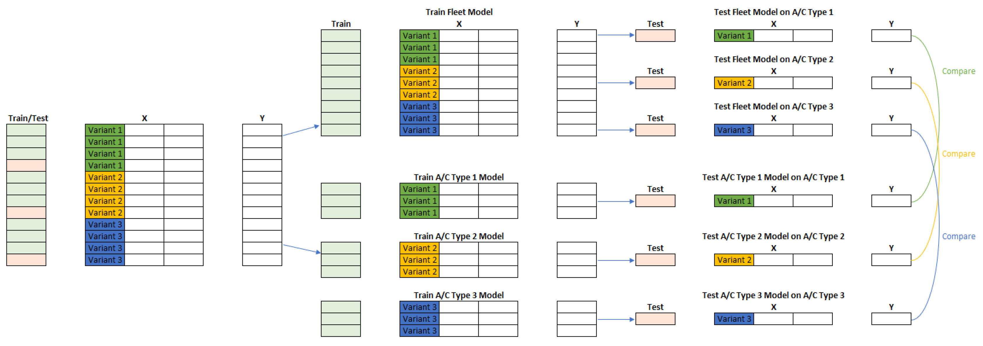
Next, a comparative analysis was conducted utilizing three distinct models to understand the advantages of TL in predictive modeling for aircraft brake wear. Initially, the optimal neural network model, described in Table 7 and identified through the HyperOpt optimization process, was trained and tested exclusively on data from Domain 1, comprising the datasets for Variants 1 and 2. This model is referred to as the standalone model for Domain 1. Following this, the same architectural framework was applied to train and assess a model on Domain 2 data (i.e., Variant 3), hereafter referred to as the standalone model for Domain 2. The results of this standalone model for Domain 2 establish the baseline against which the efficacy of the TL approach is gauged.

The performance metrics for the standalone models trained on different domains, as reported in

Table 8. Experiment 2.1: Standalone model performance on distinct domains.

Standalone Model	MAE	MSE	RMSE	R2	Training Time (s)	Prediction Time (s)
Trained on Variants 1 and 2	0.0066	0.0004	0.0197	0.6044	41.9749	0.4777
Trained on Variant 3	0.0285	0.0016	0.0396	−5.9478	2.0099	0.1040
Percentage Change	335.3767	304.9962	101.2452	−1084.142	−95.2117	−78.2391

, provide intriguing insights into the models’ predictive abilities across distinct data segments corresponding to specific variants. When evaluating the model trained and tested on Domain 1 (i.e., Variants 1 and 2) data, an MAE of 0.0066, an MSE of 0.0004, an RMSE of 0.0197, and an R² of 0.6044 are observed. These values reflect moderate predictive performance and variance explanation in the model’s output. In stark contrast, the standalone model tailored for Domain 2 (i.e., Variant 3) data exhibits a significant deterioration in performance, as indicated by a pronounced increase in error metrics: MAE increased by 335.38%, MSE by 304.99%, and RMSE by 101.25%. Most notably, the R² metric plunged to −5.95, signifying that the model’s predictions are severely out of alignment with the actual data, performing worse than a simple average. This drastic drop in R² is accompanied by a substantial reduction in training time by 95.21% and prediction time by 78.24%, reflecting the smaller dataset’s reduced complexity and size.

The percentage change between the two domains underscores the challenges in model generalization when transitioning from a larger, composite dataset to a smaller, distinct one. It highlights the need for sophisticated approaches, such as TL, to adapt models trained on abundant and varied data to perform well on limited or specific datasets without compromising prediction quality and reliability. As such, the final phase involves taking the standalone model of Domain 1 and subjecting it to the TL process, which consists of determining the optimal number of layers to freeze (from zero to two in this case)—thus retaining learned features from Domain 1—and identifying the number of new layers to introduce (up to 10), along with their respective units, to fine-tune the model for Domain 2 specifics. 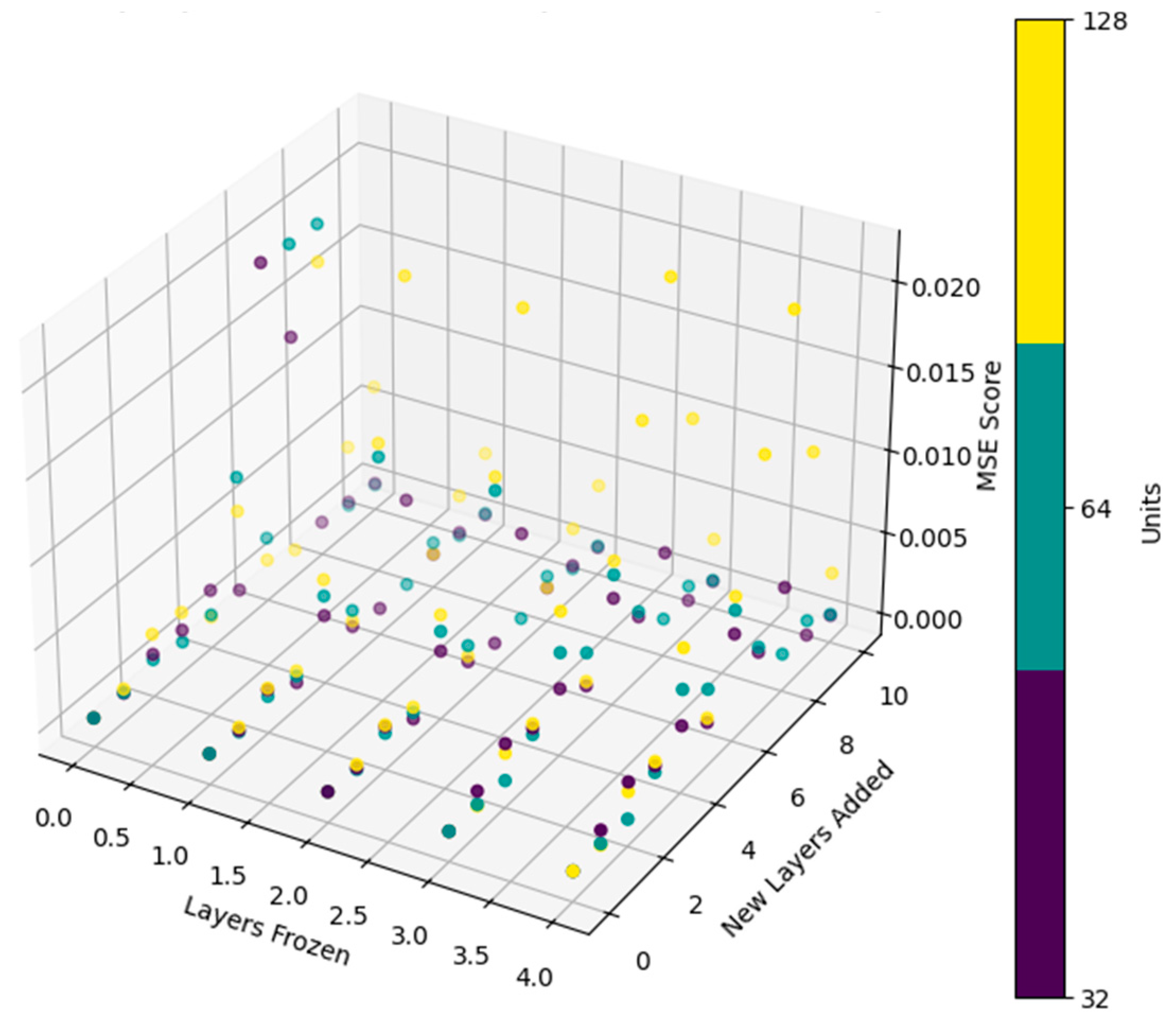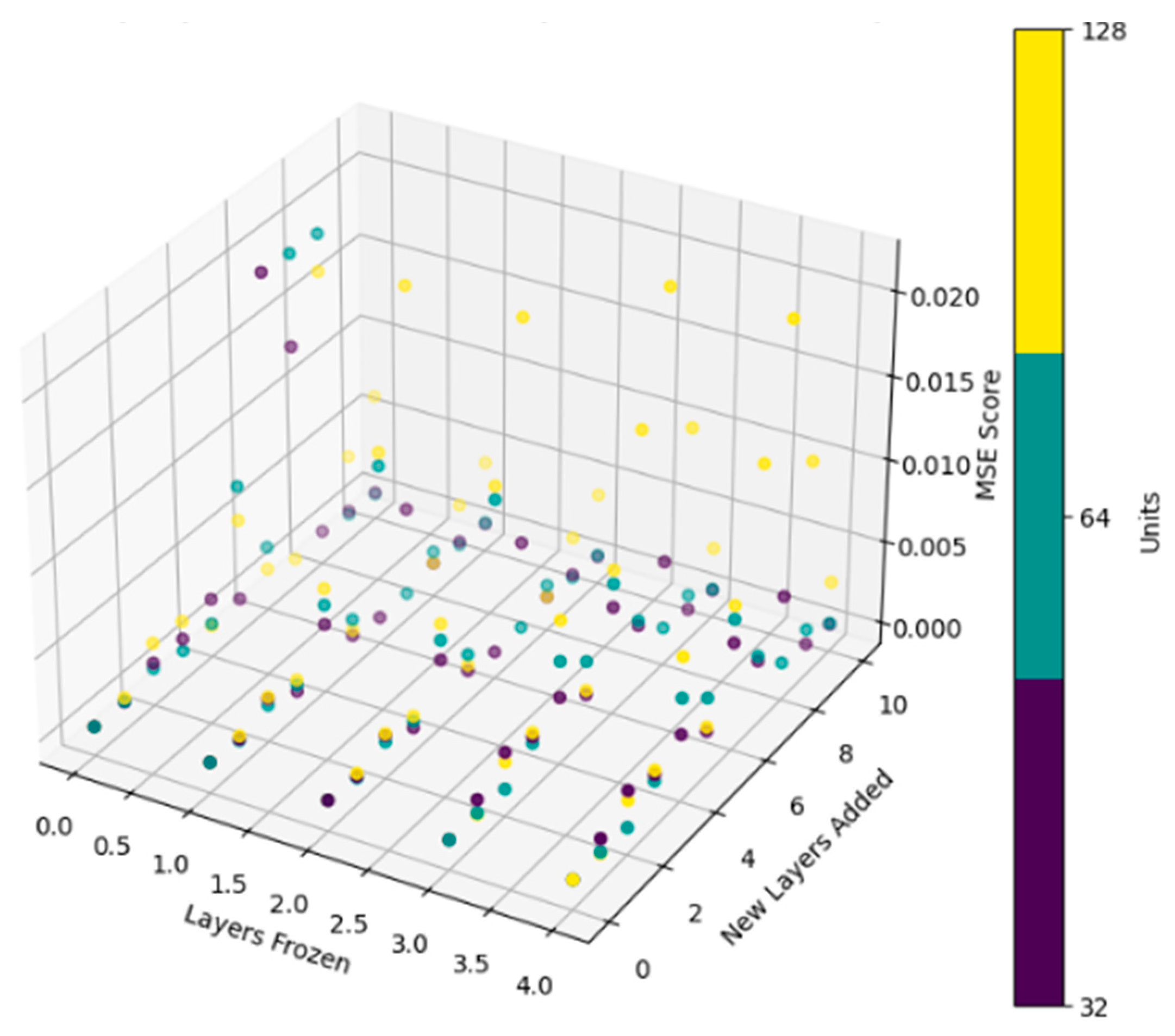Figure 9 below displays the MSE score (in percent squared, as the prediction target is percent brake wear per flight) as a function of the number of layers frozen and new layers added, with color indicating the number of units used per added layer. Note that the same units are used for each added layer, being either 32, 64, or 128. The minimum MSE found is 0.0002, obtained by freezing only the first layer and adding three new layers with 32 units each.

Upon the completion of this TL adaptation, the resulting model’s performance is rigorously compared against the baseline standalone model for Domain 2 (i.e., Variant 3) to highlight the impact of TL in enhancing model performance and generalizability across different aircraft types. The corresponding results are shown in

Table 9. Standalone model and TL model performance on Domain 2.

Model	Test Data	MAE	MSE	RMSE	R2	Training Time (s)	Prediction Time (s)
Standalone Model	Variant 3	0.0285	0.0016	0.0396	−5.9478	1.8512	0.0928
TL Model	Variant	0.0099	0.0002	0.0144	0.0802	1.7812	0.0731
Percentage Change		−65.406	−86.7619	−63.6158	−101.3491	−3.781	−21.2316

below.

Table 9 reveals a substantial improvement in all predictive performance metrics when TL is employed. Specifically, the TL model shows a remarkable decrease in MAE by 65.41%, MSE by 86.76%, and RMSE by 63.62% compared to the standalone model trained exclusively on Domain 2 data. Most critically, the R² score shifts from negative to positive, demonstrating that the TL model can explain a certain degree of variance in the data that the standalone model failed to capture. Additionally, the TL model’s training time is slightly reduced by 3.78%, and the prediction time sees a more noticeable reduction of 21.23%. This efficiency in training and prediction times, alongside the significant leap in accuracy and consistency of predictions, showcases the efficacy of TL in tuning the model to a specific, smaller dataset, enhancing its generalizability. The results also confirm the inclusion of transferable features during the pre-training phase, as poor feature engineering could have resulted in less effective knowledge transfer.

The improved performance metrics for the TL model indicate that leveraging the knowledge from Domain 1 (i.e., Variants 1 and 2) and fine-tuning for Domain 2 (i.e., Variant 3) effectively addresses the challenge posed by the smaller dataset size of the latter. TL maintains and improves the model’s predictive power, offering a more reliable, efficient, and generalizable tool for predicting aircraft brake wear. This result is a testament to the robustness of TL in applications where data may be scarce or where it is imperative to generalize across related but varied domains, such as different aircraft configurations. These findings align with trends reported in the literature for similar problems involving scarce data, where TL consistently demonstrates its ability to enhance model performance by leveraging knowledge from data-rich domains. However, this study’s significant improvement in both predictive performance and computational efficiency surpasses many reported outcomes, where TL often focuses solely on improving predictive performance without addressing operational constraints like training and prediction times. This dual improvement highlights the practical applicability of TL for real-world deployment in resource-constrained environments.

6.2.2. Experiment 2.2

In this case, the optimal model trained on Domain 1 (i.e., Variant 1) comprises five dense layers with 128, 32, 64, 32, and 1 unit, respectively, as summarized in

Table 10. Top model architecture (Variant 1).

Layer	Output Shape	Parameters
Dense	(None, 128)	11,136
Dropout	(None, 128)	0
Dense	(None, 32)	4128
Dropout	(None, 32)	0
Dense	(None, 64)	2112
Dropout	(None, 64)	0
Dense	(None, 32)	2080
Dropout	(None, 32)	0
Dense	(None, 1)	33
Trainable Parameters:		19,489

. The dropout rate is set to 11.8%, and the model is run using the Adam optimizer with a learning rate of 0.00063 and a batch size of 32 for 67 epochs. These optimal parameters were identified when HyperOpt completed 193 iterations.

The optimal model described in Table 10 is trained and tested exclusively on data from Domain 1 (i.e., Variant 1 data), forming the standalone model for Domain 1. Following this, the exact architectural framework is applied to train and assess a model on Domain 2 (i.e., Variants 2 and 3) data, referred to as the standalone model for Domain 2.

Table 11. Experiment 2.2: Standalone model performance on distinct domains.

Standalone Model	MAE	MSE	RMSE	R2	Training Time (s)	Prediction Time (s)
Trained on Variant 1	0.0036	0.0002	0.0129	0.6826	28.588	0.3444
Trained on Variants 2 and 3	0.0105	0.0007	0.0262	0.5693	19.9597	0.2212
Percentage Change	187.891	312.2437	103.0378	−16.6079	−30.1814	−35.7788

presents the comparative performance of the standalone models, emphasizing the change in predictive performance when transitioning from training on a single variant to a combined dataset of two different variants.

For the standalone model trained on Variant 1 data, the MAE is relatively low at 0.0036, and the MSE at 0.0002 reflects a strong concordance between predicted and actual values. The RMSE at 0.0129 and a relatively high R² value of 0.6826 indicate a model that fits well with the training data and explains a substantial amount of variance. However, when applying the same model configuration to the combined data of Variants 2 and 3, there is a noticeable increase in all error metrics: MAE rises by 187.89%, MSE by 312.24%, and RMSE by 103.04%. Additionally, the R² value decreases by 16.61%, indicating a decline in the model’s ability to capture variance. Additionally, both training and prediction times decrease (by 30.18% and 35.78%, respectively), likely due to the smaller cumulative dataset size for Domain 2 compared to Domain 1 (9316 samples for Variants 2 and 3 combined vs. 11,957 samples for Variant 1, as shown in Table 2). Another contributing factor could be greater homogeneity in the combined data, resulting in faster convergence during training.

The increased error metrics for Domain 2 suggest that a model optimized for a specific aircraft type does not directly translate to equally effective performance on data from different or combined variants; this reinforces the complexity inherent in aircraft performance data and the nuanced differences between various types of aircraft, even within the same model family. These results re-emphasize the need for model re-tuning or even redesign to accommodate the subtleties of a new data domain.

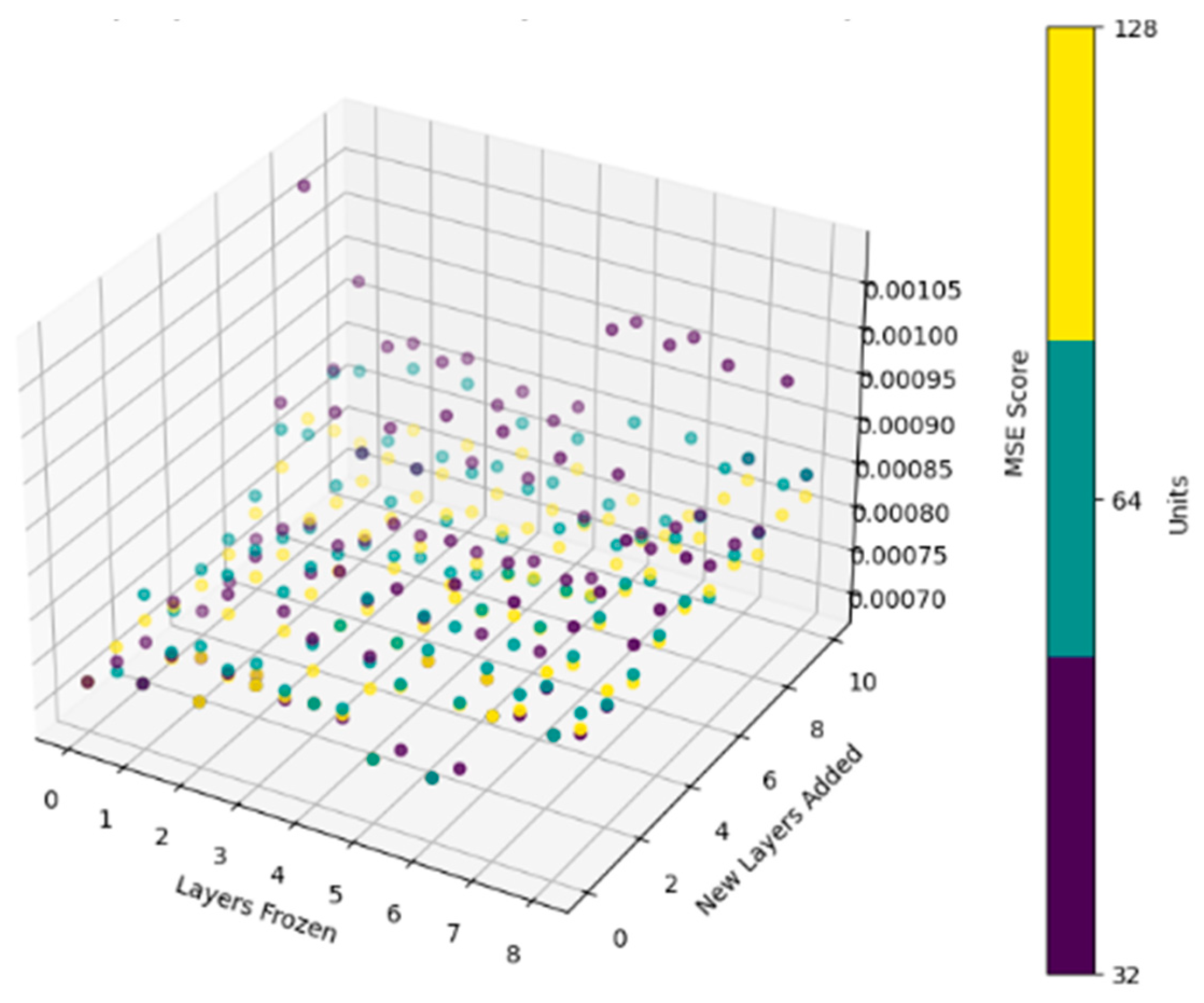
Subsequently, the standalone model of Domain 1 is subjected to the TL process, during which different numbers of layers are iteratively frozen, and the optimal number of new, additional layers and their units are identified. Figure 10 below displays the MSE score versus the number of layers frozen and added, colored by the units added for each new layer. The minimum MSE found is 0.0007, obtained by freezing none of the layers and not adding any new layers. This implies that, during the TL process, the entire model’s weights will undergo adjustment, effectively utilizing TL merely as a weight initialization scheme.

The TL model’s performance is compared against the baseline standalone model for Domain 2 (i.e., Variants 2 and 3), shown in

Table 12. Experiment 2.2: Standalone model and TL model performance on Domain 2.

Model	Test Data	MAE	MSE	RMSE	R2	Training Time (s)	Prediction Time (s)
Standalone Model	Variants 2 and 3	0.0105	0.0007	0.0262	0.5693	19.9597	0.2172
TL Model	Variants 2 and 3	0.0093	0.0007	0.0259	0.5771	10.4863	0.1749
Percentage Change		−10.983	−1.8226	−0.9155	1.3791	−47.4627	−19.4606

below.

The results in Table 12 indicate a nuanced performance enhancement when applying TL. Specifically, the MAE improved by approximately 11%, signifying a more accurate model. The MSE and RMSE saw minimal improvements of about 1.82% and 0.92%, respectively, suggesting that the TL model is slightly better at reducing the magnitude of prediction errors. A slight improvement is also observed in the R² score, which increased by approximately 1.38, indicating that the TL model explains a higher percentage of the variance in the test data for Domain 2 and providing evidence that the TL process has helped the model capture the underlying pattern in the data more effectively. Regarding computational efficiency, the training time for the TL model shows a significant reduction, nearly halving (a decrease of 47.46%), indicating a more efficient learning process likely due to the initial weights providing a better starting point. Additionally, the prediction time decreased by nearly 20%, suggesting that the TL model can make predictions more rapidly, which is an important consideration for specific DT applications where time efficiency is critical.

Overall, these results highlight that the TL model provides a slight edge over the standalone model in terms of predictive performance while offering substantial improvements in computational efficiency. Once again, this demonstrates the effectiveness of TL in refining a pre-existing model trained on one aircraft variant to better suit a related but distinct dataset corresponding to different variants, reinforcing its value as a method for enhancing model generalizability and efficiency in the predictive modeling of brake wear.

6.2.3. Experiment 2.3

In this case, the TL process is executed twice, sequentially. The optimal neural network model derived for Domain 1, corresponding to the Variant 1 dataset, forms the foundation, and its specific architectural details are listed in Table 10. Subsequently, the predefined model architecture is utilized for each domain to train and evaluate separate models, yielding standalone models for Domain 2, which encompasses the Variant 2 data, and Domain 3, pertaining to the Variant 3 data. These models are then individually assessed to determine their predictive performance;

Table 13. Experiment 2.3: Standalone model performance on distinct domains.

Standalone Model	MAE	MSE	RMSE	R2	Training Time (s)	Prediction Time (s)
Trained on Variant 1	0.0036	0.0002	0.0129	0.6826	30.1164	0.3534
Trained on Variant 2	0.0085	0.0007	0.0273	0.5419	22.8053	0.2214
Trained on Variant 3	0.0247	0.0009	0.0292	−2.7769	1.4607	0.0973

and

Table 14. Percentage change in metrics for standalone models of Domains 2 and 3.

Standalone Model	MAE % Change	MSE % Change	RMSE % Change	R2 % Change	Training Time % Change	Prediction Time % Change
Trained on Variant 2	132.781	348.5575	111.7918	−20.6139	−25.4956	−41.9432
Trained on Variant 3	579.281	414.12	126.7421	−506.794	−94.7732	−72.1505

present the results of the standalone neural network models when applied to different domains.

Table 13 provides the standalone model metrics for each domain. For Domain 1 (i.e., Variant 1), the model achieves the lowest MAE, MSE, and RMSE alongside the highest R² score, suggesting that the model fits this domain’s data well. When the model is trained and tested on Domain 2 (i.e., Variant 2), there is a noticeable uptick in the MAE and MSE and a dip in the R² score, indicating less precise predictions when compared to Domain 1. The deterioration in predictive performance becomes even more pronounced for Domain 3 (i.e., Variant 3), with the highest MAE and MSE and the lowest R² score. Table 14 provides a comparative perspective detailing the percentage changes in the performance metrics for Domains 2 and 3, using Domain 1 as the benchmark. The metrics exhibit substantial increases in the MAE and MSE for Domains 2 and 3, implying that the model’s error rates inflate when transferred to these domains; this proves that the Domain 1 model is less suited to capturing the brake wear dynamics of the subsequent domains without adjustment. The percentage change in the R² score for Domain 3 is particularly striking, declining by over 500%. This stark decrease is a clear indicator that the model, while adequate for the dataset of Variant 1, fails to generalize effectively to the significantly different conditions or operational parameters of Variant 3. Additionally, the percentage changes in training and prediction times highlight a reduction in time for Domains 2 and 3, likely due to their smaller data sizes that require less computational effort.

These results underscore the criticality of domain-specific nuances in predictive modeling. While a model may exhibit robust performance in one domain, its performance can vary significantly when applied to another, emphasizing the need for adaptive modeling approaches—such as TL—that allow models to adjust to variations in data distributions, operational conditions, and feature relevance across different domains. As such, the standalone model of Domain 1 is subjected to the TL process, which determines the optimal number of layers to freeze and the number of new layers to add along with their units, to fine-tune the model for Domain 2. 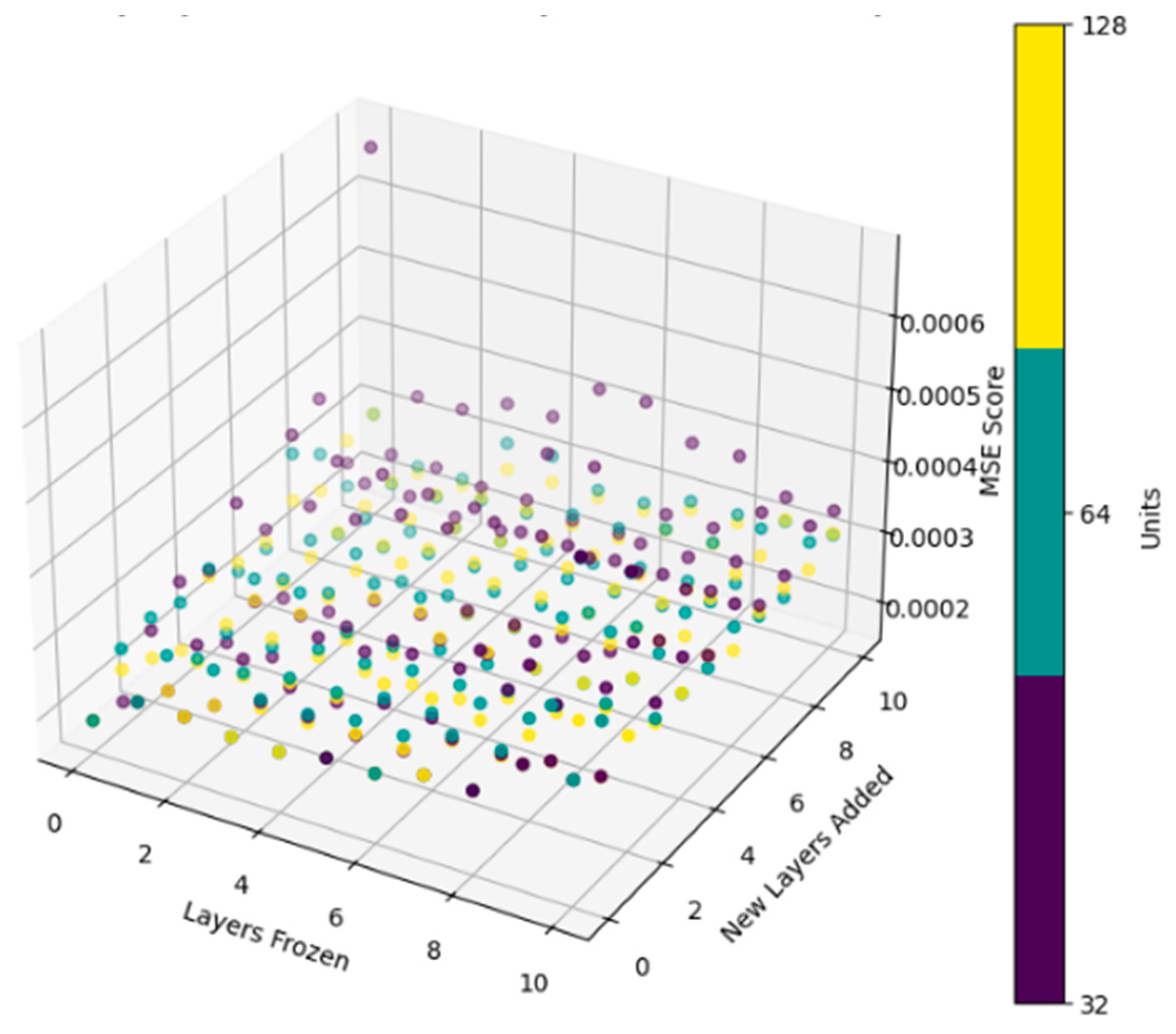Figure 11 below displays the MSE score versus the number of layers frozen and added, colored by the units added for each new layer. The minimum MSE across all units is 0.0007, obtained by freezing none of the layers (i.e., weight initialization) and adding four new layers with 32 units each.

Upon completion of this TL adaptation, the resulting model’s performance is rigorously compared against the baseline standalone model for Domain 2 (i.e., Variant 2) to highlight the impact of TL in enhancing model generalizability to Domain 2. The corresponding results are shown in

Table 15. Experiment 2.3: Standalone model and TL model performance on Domain 2.

Model	Test Data	MAE	MSE	RMSE	R2	Training Time (s)	Prediction Time (s)
Standalone Model	Variant 2	0.0085	0.0007	0.0273	0.5419	23.9201	0.2358
TL Model 1	Variant 2	0.0093	0.0007	0.0263	0.5733	30.7548	0.2299
Percentage Change		10.2780	0	−3.4848	5.7889	28.5732	−2.5184

below.

Table 15 compares the performance metrics between the standalone model and the TL model, both tested on Domain 2 data (i.e., Variant 2). The MAE increases by 10.28%, suggesting that, despite the adaptation process, the TL model exhibited a slight decrease in accuracy regarding average prediction errors compared to the standalone model trained directly on Domain 2. MSE and RMSE show minimal changes, with MSE remaining unchanged and RMSE reducing slightly by 3.48%; this indicates a minor improvement in the TL model’s ability to mitigate significant errors, reflected in a slightly more consistent performance despite the higher error rates overall. There is also an improvement in the R² score, which increases by 5.79%, indicating that the TL model is better at explaining the variability in the dataset relative to the standalone model. Regarding computational efficiency, the training time for the TL model increased by 28.57%, indicating more computational resources were needed, likely due to the complexity introduced by the TL process (i.e., added layers). Additionally, the prediction time saw a marginal decrease of 2.52%, representing a slightly faster inference time.

The TL model is subsequently fine-tuned once more to adapt it specifically for Domain 3 (i.e., Variant 3). Figure 12 shows the MSE score for different quantities of frozen and added layers. The minimum MSE on Domain 3 is found by freezing 16 layers of the previous TL model and adding eight new layers with 32 units each.

Table 16. Experiment 2.3: Standalone model and final TL model performance on Domain 3.

Model	Test Data	MAE	MSE	RMSE	R2	Training Time (s)	Prediction Time (s)
Standalone Model	Variant 3	0.0247	0.0009	0.0292	−2.7769	1.6781	0.0989
TL Model 2	Variant 3	0.0105	0.0002	0.0146	0.0594	2.9543	0.0985
Percentage Change		−57.6843	−75.0973	−50.0974	102.1408	76.0518	−0.4349

shows the final TL model’s performance on Domain 3 compared to that of the standalone model for the same domain.

Table 16 delineates the comparative outcomes of the final TL model and the standalone model when applied to Domain 3 (i.e., Variant 3). Results show that the TL model significantly outperforms the standalone model tailored to the same domain across several critical performance metrics. It reduces the MAE by 57.68%, indicating a substantial improvement in the average magnitude of the errors and demonstrating the TL model’s enhanced capability to predict closer to the actual values. The MSE decreases by 75.10% and the RMSE by 50.10%, highlighting the TL model’s ability to reduce significant errors. There is an increase in the R² score by 102.14%; this dramatic shift from a negative to a positive value indicates that the TL model explains a positive variance in the dataset, unlike the standalone model, which performed worse than a simple average model.

Regarding computational effort, the training time for the TL model increases by 76.05%, reflecting an additional computational burden, likely due to the complexity of the TL process in this case. The prediction time remains almost unchanged, with a negligible decrease of 0.43%. These results affirm that the TL process has effectively leveraged the knowledge gained from the broader datasets of Domains 1 and 2 to enhance the model’s performance on the more challenging Domain 3 dataset. The stark improvements in error metrics and the R² score particularly underscore the value of employing TL to address challenges posed by limited data diversity and volume, as with the dataset corresponding to Variant 3.

To complete the analysis,

Table 17. Experiment 2.3: Standalone model and final TL model performance on Domain 2.

Model	Test Data	MAE	MSE	RMSE	R2	Training Time (s)	Prediction Time (s)
Standalone Model	Variant 2	0.0085	0.0007	0.0273	0.5419	22.6949	0.2042
TL Model 2	Variant 2	0.0224	0.0018	0.0422	−0.0981	2.7953	0.2183
Percentage Change		164.2796	139.7229	54.8299	−118.108	−87.6832	6.9292

contrasts the performance metrics of the standalone model and the final TL model on Domain 2 (i.e., Variant 2), after the TL process was applied to fine-tune the model to Domain 3 data. Note that all TL models were evaluated and compared to the standalone models on the respective target domains.

The results in Table 17 show a stark divergence in performance compared to the earlier adaptation, with significant regressions in the TL model’s performance metrics. MAE increased dramatically by 164.28%, indicating that the adjustments made to suit Domain 3 better have adversely affected the model’s accuracy on Domain 2. The MSE and RMSE show similar trends, with increases of 139.72% and 54.83%, respectively, confirming that the model’s predictive performance deteriorated for Domain 2. The R2 score declines from a moderately positive value of 0.5419 to −0.0981, a change of −118.11%. This drastic decrease indicates that the model’s ability to explain the variability in the dataset for Domain 2 has become worse than a model that would merely predict the mean of the target values.

Regarding computational efficiency, the training time was reduced by 87.68%, indicating a quicker training phase. The prediction time saw a slight increase of about 6.93%, which, although minimal, indicates that the model requires slightly more computation time for predictions despite its reduced accuracy and effectiveness.

These results illustrate that while the TL model optimized for Domain 3 has improved its performance on that specific dataset, its generalization to Domain 2 has suffered significantly, highlighting a critical challenge in TL applications: optimizing a model for one domain may significantly degrade its performance on another when the domains differ substantially in characteristics or data distribution. This necessitates careful consideration and potentially more bespoke tuning for each domain, ensuring that improvements in one area do not undermine performance elsewhere.

6.2.4. Experiment 2.4

In this scenario, Domain 1 is taken as the data corresponding to Variant 2, which are slightly smaller than those of Variant 1 (as detailed in Table 2). The optimal model identified through HyperOpt for Variant 2 data consists of six dense layers with 128, 128, 256, 128, 32, and 1 unit, respectively, shown in

Table 18. Top model architecture (Variant 2).

Layer	Output Shape	Parameters
Dense	(None, 128)	11,136
Dropout	(None, 128)	0
Dense	(None, 128)	16,512
Dropout	(None, 128)	0
Dense	(None, 256)	33,024
Dropout	(None, 256)	0
Dense	(None, 128)	32,896
Dropout	(None, 128)	0
Dense	(None, 32)	4128
Dropout	(None, 32)	0
Dense	(None, 1)	33
Trainable Parameters:		97,729

. The dropout rate is set to 13.2%, and the model is run using the Adam optimizer with a learning rate of 0.00068 a batch size of 64, and it is trained for 90 epochs. These optimal parameters were identified when HyperOpt completed 100 evaluations.

The above optimal model is trained and tested exclusively on data from Domain 1 (i.e., Variant 2 data). The exact architectural framework is then applied to train and assess the model on Domain 2 (i.e., Variants 1 and 3) data.

Table 19. Experiment 2.4: Standalone model performance on distinct domains.

Standalone Model	MAE	MSE	RMSE	R2	Training Time (s)	Prediction Time (s)
Trained on Variant 2	0.0096	0.0007	0.0258	0.5919	21.6417	0.2478
Trained on Variants 1 and 3	0.0044	0.0002	0.0143	0.6058	32.5148	0.3799
Percentage Change	−54.3329	−69.1718	−44.4769	2.3503	50.2416	53.3045

presents a comparative performance of these standalone models.

The comparative analysis reflected in Table 19 outlines the performance of the standalone models, whose architectures were optimized for Domain 1 (i.e., Variant 2 data). The standalone model trained on Domain 1 shows an MAE of 0.0096, an MSE of 0.0007, and an RMSE of 0.0258, with an R² score of 0.5919. These metrics imply reasonable predictive performance.

Interestingly, a performance improvement is observed when the same model structure is applied to Domain 2, combining data from Variants 1 and 3. The MAE drops significantly by approximately 54.33%, while the MSE and RMSE decrease by 69.17% and 44.48%, respectively, suggesting that the model trained on Domain 2 makes fewer significant errors in its predictions. Moreover, the R² score slightly improves, increasing by 2.35%, showing that the Domain 2 model captures a marginally higher percentage of variance than the Domain 1 model. The improvements in these performance metrics demonstrate that the combined data of Variants 1 and 3 may offer a richer representation of the underlying brake wear patterns and a broader spectrum of operational conditions, helping the model learn more effectively. On the other hand, training and prediction times increase for the Domain 2 model by 50.24% and 53.30%, respectively; this is likely due to the larger combined dataset of Domain 2, which demands more computational resources for training and inference. These results emphasize the importance of comprehensive datasets encompassing various conditions to train models with improved generalization capabilities for predictive maintenance applications.

Still, the standalone model of Domain 1 is subjected to the TL process, where different numbers of layers are frozen and new layers are added. Figure 13 below shows the MSE score by the number of layers frozen and added, colored by the units for each new layer. The minimum MSE found is 0.0002, obtained by freezing none of the layers and adding one new layer with 32 units.

The TL model’s performance is compared against the baseline standalone model for Domain 2 (Variant 1 and Variant 3), shown in

Table 20. Experiment 2.4: Standalone model and TL model performance on Domain 2.

Model	Test Data	MAE	MSE	RMSE	R2	Training Time (s)	Prediction Time (s)
Standalone Model	Variants 1 and 3	0.0044	0.0002	0.0143	0.6058	32.1935	0.3367
TL Model	Variants 1 and 3	0.0071	0.0002	0.0134	0.6519	34.3042	0.3136
Percentage Change		61.6925	0	−6.0299	7.6100	6.5561	−6.8405

below.

The standalone model’s performance on Domain 2 already demonstrates strong predictive capabilities, capturing over 60% of the variance in the target variable. After applying TL, the model sees a 61.69% increase in MAE and a 7.61% improvement in R², while MSE remains constant and RMSE improves by a slight 6.03%. Notably, the rise in MAE suggests that, on average, the TL model predictions are further from the actual values than those of the standalone model. However, the R² score improvement indicates that despite the more significant average errors, the TL model is better at fitting the variability in the data than the standalone model. The enhancement in the R² score and the slight reduction in RMSE point towards the TL model’s enhanced ability to model the variance within the combined dataset, even if it occasionally makes higher errors. This underscores the balance between achieving lower error rates and capturing the data’s underlying structure.

The training time for the TL model is about 6.56% higher than that of the standalone model, while the prediction time shows a modest improvement of approximately 6.84%. These shifts in computational performance are minor but reveal that the TL process, particularly with adding a new layer, necessitates slightly more time for training, which is a reasonable trade-off considering that the data size for Domain 2 is larger than that for Domain 1. While the TL model does not uniformly surpass the standalone model across all metrics, it showcases its strength in capturing the complex variance of the data, thereby suggesting that it could be a more reliable choice in varied real-world scenarios, even if it incurs slightly higher errors on average.

The aforementioned four experiments were conducted to assess the ability of TL to adapt a model developed on one domain comprising specific aircraft configurations to another, highlighting its potential to improve predictive performance across varied datasets. The results underscore the value of utilizing advanced modeling techniques like TL to ensure that predictive models remain robust and reliable across different aircraft types and their varying operating conditions, enhancing the models’ practical utility in real-world applications. Among Experiments 2.1–2.4, Experiment 2.1 demonstrated the most effective use of TL to enhance model generalizability as it showcased a substantial improvement in all performance metrics when TL was applied, particularly in minimizing MAE, MSE, and RMSE, alongside a pronounced shift from a negative to a positive R² score. These results indicate that the TL model became more accurate and more capable of capturing the variance of the smaller, specific dataset of Variant 3 compared to the standalone model. This adaptability is important for predictive performance in diverse operational scenarios like different variants of a particular widebody aircraft.

The critical takeaway from these experiments is that TL can significantly enhance a model’s generalizability and predictive accuracy when properly tuned, particularly in fields like aviation, where operational conditions can vary widely between datasets. These results also suggest that the sequence of domains on which the model is trained significantly influences the effectiveness of TL. For instance, starting with a domain that offers greater data diversity or encompasses a broader spectrum of operational conditions (e.g., Variants 1 and 2 combined) provides a stronger foundation for generalization. This ensures that the model learns more comprehensive and transferable features, which can then be fine-tuned for smaller, more specific domains like Variant 3. Conversely, starting with a less diverse or more narrowly focused domain may limit the model’s ability to capture generalizable patterns, making subsequent adaptation through TL less effective. Therefore, the choice and sequence of training domains should be strategically aligned with the data’s characteristics and the desired application to maximize the benefits of TL.

7. Conclusions and Future Work

This study explored the necessity and advantages of model generalizability, as well as the potential of TL to improve predictive models for wear-prone components such as aircraft carbon brakes. The research focused on datasets representative of different variants of a widebody aircraft. The findings are particularly valuable for DT applications, where robust and reliable predictive models are crucial for real-time monitoring, analysis, and decision-making to optimize maintenance and operational performance.

Experiment 1 evaluated the performance of a generalized fleet-based model against specialized models for each aircraft variant. The results demonstrated that a well-optimized generalized model could deliver robust performance across different aircraft types, effectively accommodating fleet-wide variations when trained on diverse and sufficient data. This approach streamlines predictive maintenance strategies by eliminating the need for multiple specialized models, significantly reducing the computational overhead and complexity associated with managing them. By fostering efficient model development and maintenance, generalization enhances operational efficiency and delivers substantial cost savings.

Experiment 2 investigated the potential of TL to enhance model generalizability across domains, defined as data subsets representing diverse aircraft configurations. Four distinct cases were examined, with TL applied to transfer knowledge from one domain to another using different combinations of aircraft variants as starting and target tasks. Strategies such as weight initialization and feature extraction were employed, involving freezing specific layers of pre-trained models and adding new trainable layers to fine-tune them for target domains. These methods allowed the models to retain knowledge from broader datasets while capturing the unique characteristics of smaller, more specialized datasets.

TL demonstrated notable success in improving model performance, particularly for less representative datasets like Variant 3. For instance, starting with a domain offering greater data diversity or a broader spectrum of operational conditions (e.g., Variants 1 and 2 combined) provided a stronger foundation for generalization. This ensured the model could learn comprehensive, transferable features, which were fine-tuned to adapt effectively to smaller, highly specific domains like Variant 3. In cases of scarce or highly specific data, TL maintained predictive reliability while enhancing model adaptability and efficiency across varying datasets. This experiment also highlighted the efficacy of TL in improving performance while reducing the time and data required to develop high-performing models.

Both experiments highlight the strategic use of data and training methodologies to enhance predictive performance while optimizing computational resources. Leveraging generalized models or employing TL reduces the need for extensive retraining when new data become available, or when models are applied to slightly different contexts. This approach is particularly valuable when data collection is challenging or costly, allowing for an efficient use of existing datasets and resources. By streamlining model development and adaptation, these methods offer a cost-effective and practical solution for deploying predictive models in real-world applications.

Such techniques have practical implications for maintenance scheduling and operational planning. The enhanced performance and reliability of predictive models provide a solid foundation for optimizing maintenance schedules, ensuring a better allocation of resources such as personnel or spare parts. By reducing unplanned downtime, airlines can improve aircraft availability and minimize disruptions to flight schedules. In addition to operational benefits, improved model reliability contributes to safety by proactively identifying potential issues before they escalate, thus mitigating associated risks.

The results provide a foundation for further exploration into integrating ML with diverse data sources, such as datasets from different aircraft types or airlines, and incorporating advanced modeling techniques. TL could also be extended to other data segments, such as transitioning from low-wear to high-wear scenarios, to enhance the predictive performance of regression models. Also, given that the success of generalizable models (whether using TL or not) relies heavily on selecting features that effectively capture brake wear across varied aircraft types and operating conditions, future research should investigate the impact of different feature subsets or alternative feature engineering approaches. For example, improving the prediction of continuous brake wear values might involve adopting a more granular approach, such as using per-flight data without condensation (i.e., avoiding the averaging of features over constant segments of the original wear pin signal) or directly leveraging the raw 1 Hz CPL data. In particular, the underperformance observed for Variant 3—due to its limited data availability—highlights the need for more expressive and robust features. Future work could explore feature enrichment strategies to address this, such as synthetic data augmentation, the incorporation of higher-resolution sensor data (if available), or engineering physics-informed features that are invariant across aircraft types but still sensitive to wear progression. These techniques may help compensate for the lack of direct training data by improving the model’s ability to generalize from richer domains to smaller, underrepresented ones like Variant 3.

Future research could also explore combining TL with real-time data streams to enable dynamic model updates as new information becomes available, further enhancing the adaptability and performance of predictive maintenance systems. Testing these models in real operational environments would validate their practical utility and provide opportunities for refinement based on real-world data and feedback. Furthermore, the applicability of these findings could extend to other aircraft components or industries, such as the automotive industry, thereby broadening the impact of these strategies.

Integrating domain knowledge from aerospace engineering with advanced ML techniques could lead to the development of physics-informed models. These models would not only enhance predictive capabilities but also improve interpretability by aligning predictions with the physical principles governing the systems they monitor. Such interdisciplinary approaches hold the potential to create more robust, accurate, and actionable solutions for predictive maintenance, ultimately contributing to safer and more efficient operations.

This research confirms the value of using sophisticated ML techniques to enhance predictive maintenance strategies, emphasizing the importance of model generalizability and TL’s strategic use. Future work will continue to refine these approaches, ensuring they remain adaptable and practical as new challenges and data environments emerge.

References

1. Daily, J.; Peterson, J. Predictive Maintenance: How Big Data Analysis Can Improve Maintenance. In Supply Chain Integration Challenges in Commercial Aerospace; Richter, K., Walther, J., Eds.; Springer: Cham, Switzerland, 2017; pp. 267–278. [Google Scholar] [CrossRef]
2. Stanton, I.; Munir, K.; Ikram, A.; El-Bakry, M. Predictive Maintenance Analytics and Implementation for Aircraft: Challenges and Opportunities. Syst. Eng. 2023, 26, 216–237. [Google Scholar] [CrossRef]
3. Korvesis, P. Machine Learning for Predictive Maintenance in Aviation. Ph.D. Thesis, Université Paris-Saclay (COmUE), Paris, France, 2017. Available online: https://hal.science/tel-02003508 (accessed on 5 June 2025).
4. Errandonea, I.; Beltrán, S.; Arrizabalaga, S. Digital Twin for Maintenance: A Literature Review. Comput. Ind. 2020, 123, 103316. [Google Scholar] [CrossRef]
5. Thelen, A.; Zhang, X.; Fink, O.; Hehenberger, P.; Ríos, J.; Rutter, B.; Boschert, S. A Comprehensive Review of Digital Twin—Part 1: Modeling and Twinning Enabling Technologies. Struct. Multidiscip. Optim. 2022, 65, 354. [Google Scholar] [CrossRef]
6. Liu, H.; Xia, M.; Williams, D.; Sun, J.; Yan, H. Digital Twin-Driven Machine Condition Monitoring: A Literature Review. J. Sens. 2022, 2022, 6129995. [Google Scholar] [CrossRef]
7. Arthur, R.; French, M.; Ganguli, J.; Kinard, D.A.; Kraft, E.; Marks, I.; Matlik, J.; Fischer, O.; Sangid, M.; Seal, D.; et al. Digital Twin: Definition & Value—AIAA and AIA Position Paper; AIAA Digital Engineering Integration Committee: Reston, VA, USA, 2020. [Google Scholar]
8. Pinon Fischer, O.J.; Matlik, J.F.; Schindel, W.D.; French, M.O.; Kabir, M.H.; Ganguli, J.S.; Hardwick, M. Digital Twin: Reference Model, Realizations, and Recommendations. Insight 2022, 25, 50–55. [Google Scholar] [CrossRef]
9. AIAA Digital Engineering Integration Committee (DEIC). Digital Twin: Reference Model, Realizations & Recommendations; AIAA: Reston, VA, USA; AIA: Washington, DC, USA; NAFEMS: Glasgow, UK, 2023. [Google Scholar]
10. Pinon Fischer, O.J.; Sabri, S.; Chen, Y. Fundamentals of Digital Twins, Modeling Approaches, and Governance. In Digital Twin—Fundamentals and Applications; Sabri, S., Alexandridis, K., Lee, N., Eds.; Springer: Cham, Switzerland, 2024; Chapter 2. [Google Scholar] [CrossRef]
11. Maleki, F.; Ovens, K.; Gupta, R.; Reinhold, C.; Spatz, A.; Forghani, R. Generalizability of Machine Learning Models: Quantitative Evaluation of Three Methodological Pitfalls. Radiol. Artif. Intell. 2022, 5, e220028. [Google Scholar] [CrossRef] [PubMed]
12. Ying, X. An Overview of Overfitting and Its Solutions. J. Phys. Conf. Ser. 2019, 1168, 022022. [Google Scholar] [CrossRef]
13. Li, Q.; Peng, Z.; Feng, L.; Zhang, Q.; Xue, Z.; Zhou, B. MetaDrive: Composing Diverse Driving Scenarios for Generalizable Reinforcement Learning. IEEE Trans. Pattern Anal. Mach. Intell. 2023, 45, 3461–3475. [Google Scholar] [CrossRef]
14. Xu, W.; He, J.; Shu, Y. Transfer Learning and Deep Domain Adaptation. In Advances and Applications in Deep Learning; IntechOpen: London, UK, 2020. [Google Scholar] [CrossRef]
15. Tan, C.; Sun, F.; Kong, T.; Zhang, W.; Yang, C.; Liu, C. A Survey on Deep Transfer Learning. In Artificial Neural Networks and Machine Learning—ICANN 2018: 27th International Conference on Artificial Neural Networks, Rhodes, Greece, 4–7 October 2018; Proceedings, Part III; Kůrková, V., Manolopoulos, Y., Hammer, B., Iliadis, L., Maglogiannis, I., Eds.; Springer: Cham, Switzerland, 2018; Volume 11141, pp. 270–279. [Google Scholar] [CrossRef]
16. Weiss, K.; Khoshgoftaar, T.M.; Wang, D. A Survey of Transfer Learning. J. Big Data 2016, 3, 9. [Google Scholar] [CrossRef]
17. Kouw, W.M.; Loog, M. An Introduction to Domain Adaptation and Transfer Learning. arXiv 2018, arXiv:1812.11806. [Google Scholar] [CrossRef]
18. Pan, S.J.; Yang, Q. A Survey on Transfer Learning. IEEE Trans. Knowl. Data Eng. 2010, 22, 1345–1359. [Google Scholar] [CrossRef]
19. Oikonomou, A.; Loutas, T.; Eleftheroglou, N.; Freeman, F.; Zarouchas, D. Remaining Useful Life Prognosis of Aircraft Brakes. Int. J. Progn. Health Manag. 2022, 13, 1–11. [Google Scholar] [CrossRef]
20. Choudhuri, K.; Shekhar, A. Predicting Brake Pad Wear Using Machine Learning; iGloble Software Solutions: New Delhi, India, 2020. [Google Scholar] [CrossRef]
21. Harish, S.; Jegadeeshwaran, R.; Sakthivel, G. Brake Health Prediction Using LogitBoost Classifier Through Vibration Signals: A Machine Learning Framework. Int. J. Progn. Health Manag. 2021, 12, 2. [Google Scholar] [CrossRef]
22. Küfner, T.; Döpper, F.; Müller, D.; Trenz, A.G. Predictive Maintenance: Using Recurrent Neural Networks for Wear Prognosis in Current Signatures of Production Plants. Int. J. Mech. Eng. Robot. Res. 2021, 10, 583–591. [Google Scholar] [CrossRef]
23. Magargle, R.; Johnson, L.; Mandloi, P.; Davoudabadi, P.; Kesarkar, O.; Krishnaswamy, S.; Batteh, J.; Pitchaikani, A. A Simulation-Based Digital Twin for Model-Driven Health Monitoring and Predictive Maintenance of an Automotive Braking System. In Proceedings of the 12th International Modelica Conference, Prague, Czech Republic, 15–17 May 2017; Linköping University Electronic Press: Linköping, Sweden, 2017; pp. 235–244. [Google Scholar] [CrossRef]
24. Gerardi, T.G. Health Monitoring Aircraft. J. Intell. Mater. Syst. Struct. 1990, 1, 375–385. [Google Scholar] [CrossRef]
25. Puranik, T.G. A Methodology for Quantitative Data-Driven Safety Assessment for General Aviation. Ph.D. Thesis, Georgia Institute of Technology, Atlanta, GA, USA, 2018. [Google Scholar]
26. Krajček, K.; Nikolić, D.; Domitrović, A. Aircraft Performance Monitoring from Flight Data. Teh. Vjesn. 2015, 22, 1337–1344. [Google Scholar] [CrossRef]
27. Samaranayake, P.; Kiridena, S. Aircraft Maintenance Planning and Scheduling: An Integrated Framework. J. Qual. Maint. Eng. 2012, 18, 432–453. [Google Scholar] [CrossRef]
28. Vidović, A.; Franjić, A.; Štimac, I.; Ozmec Ban, M. The Importance of Flight Recorders in the Aircraft Accident Investigation. Transp. Res. Procedia 2022, 64, 183–190. [Google Scholar] [CrossRef]
29. Li, L. Anomaly Detection in Airline Routine Operations Using Flight Data Recorder Data. Master’s Thesis, Massachusetts Institute of Technology, Cambridge, MA, USA, 2013. Available online: http://hdl.handle.net/1721.1/82498 (accessed on 5 June 2025).
30. Chati, Y.S.; Balakrishnan, H. Aircraft Engine Performance Study Using Flight Data Recorder Archives. In Proceedings of the 2013 Aviation Technology, Integration, and Operations Conference, Los Angeles, CA, USA, 12–14 August 2013; AIAA: Reston, VA, USA, 2013. [Google Scholar] [CrossRef]
31. FlightAware®. About FlightAware®. 2023. Available online: https://flightaware.com/about/ (accessed on 5 June 2025).
32. Drone Pilot Ground School. How to Read an Aviation Routine Weather (METAR) Report. 2023. Available online: https://www.dronepilotgroundschool.com/reading-aviation-routine-weather-metar-report/ (accessed on 5 June 2025).
33. Mackenzie, A. The Production of Prediction: What Does Machine Learning Want? Eur. J. Cult. Stud. 2015, 18, 429–445. [Google Scholar] [CrossRef]
34. Ho, S.Y.; Phua, K.; Wong, L.; Bin Goh, W.W. Extensions of the External Validation for Checking Learned Model Interpretability and Generalizability. Patterns 2020, 1, 100129. [Google Scholar] [CrossRef]
35. Puranik, T.G.; Rodriguez, N.; Mavris, D.N. Towards Online Prediction of Safety-Critical Landing Metrics in Aviation Using Supervised Machine Learning. Transp. Res. Part C Emerg. Technol. 2020, 120, 102819. [Google Scholar] [CrossRef]
36. Goodfellow, I.; Bengio, Y.; Courville, A. Deep Learning; MIT Press: Cambridge, MA, USA, 2016. [Google Scholar]
37. Benesty, J.; Chen, J.; Huang, Y.; Cohen, I. Pearson Correlation Coefficient. In Noise Reduction in Speech Processing; Benesty, J., Chen, J., Huang, Y., Cohen, I., Eds.; Springer: Berlin/Heidelberg, Germany, 2009; Volume 2, pp. 1–4. [Google Scholar] [CrossRef]
38. García, S.; Luengo, J.; Herrera, F. Data Preprocessing in Data Mining; Springer: Cham, Switzerland, 2015; Volume 72. [Google Scholar] [CrossRef]
39. Kang, H. The Prevention and Handling of the Missing Data. Korean J. Anesthesiol. 2013, 64, 402–406. [Google Scholar] [CrossRef] [PubMed]
40. Kaya, E. Spline Interpolation Techniques. J. Tech. Sci. Technol. 2013, 2, 47–52. [Google Scholar] [CrossRef]
41. Maeland, E. On the Comparison of Interpolation Methods. IEEE Trans. Med. Imaging 1988, 7, 213–217. [Google Scholar] [CrossRef]
42. Habermann, C.; Kindermann, F. Multidimensional Spline Interpolation: Theory and Applications. Comput. Econ. 2007, 30, 153–169. [Google Scholar] [CrossRef]
43. Blu, T.; Thévenaz, P.; Unser, M. Linear Interpolation Revitalized. IEEE Trans. Image Process. 2004, 13, 710–719. [Google Scholar] [CrossRef]
44. Chai, T.; Draxler, R.R. Root Mean Square Error (RMSE) or Mean Absolute Error (MAE)?–Arguments against Avoiding RMSE in the Literature. Geosci. Model Dev. 2014, 7, 1247–1250. [Google Scholar] [CrossRef]
45. Acuna, E.; Rodriguez, C. A Meta-Analysis Study of Outlier Detection Methods in Classification; Technical Report; Department of Mathematics, University of Puerto Rico at Mayagüez: Mayagüez, Puerto Rico, USA, 2004. [Google Scholar]
46. Pedregosa, F.; Varoquaux, G.; Gramfort, A.; Michel, V.; Thirion, B.; Grisel, O.; Blondel, M.; Prettenhofer, P.; Weiss, R.; Dubourg, V.; et al. Scikit-learn: Machine Learning in Python. J. Mach. Learn. Res. 2011, 12, 2825–2830. [Google Scholar]
47. Reitermanová, Z. Data Splitting. In WDS’10 Proceedings of Contributed Papers, Part I; Charles University, Faculty of Mathematics and Physics: Prague, Czech Republic, 2010; pp. 31–36. ISBN 978-80-7378-139-2. [Google Scholar]
48. Bergstra, J.; Komer, B.; Eliasmith, C.; Yamins, D.; Cox, D.D. Hyperopt: A Python Library for Model Selection and Hyperparameter Optimization. Comput. Sci. Discov. 2015, 8, 014008. [Google Scholar] [CrossRef]
49. Komer, B.; Bergstra, J.; Eliasmith, C. Hyperopt-Sklearn: Automatic Hyperparameter Configuration for Scikit-Learn. In Proceedings of the 13th Python in Science Conference, Austin, TX, USA, 6–12 July 2014; Citeseer: Austin, TX, USA, 2014. [Google Scholar]
50. Komer, B.; Bergstra, J.; Eliasmith, C. Hyperopt-sklearn. In Automated Machine Learning: Methods, Systems, Challenges; Hutter, F., Kotthoff, L., Vanschoren, J., Eds.; Springer: Cham, Switzerland, 2019; pp. 97–111. [Google Scholar] [CrossRef]
51. Botchkarev, A. Performance Metrics (Error Measures) in Machine Learning Regression, Forecasting and Prognostics: Properties and Typology. Interdiscip. J. Inf. Knowl. Manag. 2019, 14, 45–79. [Google Scholar] [CrossRef]
52. DataTechNotes. Regression Accuracy Check in Python (MAE, MSE, RMSE, R-Squared). 2019. Available online: https://www.datatechnotes.com/2019/10/accuracy-check-in-python-mae-mse-rmse-r.html (accessed on 5 June 2025).
Figure 1. Sample signals from CPL data.
Aerospace 12 00555 g001
Figure 2. Sample routine METAR [32].
Aerospace 12 00555 g002
Figure 3. Brake degradation profiles (a) and histogram of degradations per flight (b) for various aircraft types.
Aerospace 12 00555 g003
Figure 4. Methodology overview for Experiment 1.
Aerospace 12 00555 g004
Figure 5. Overview of methodology to assess TL potential to improve model generalizability (Experiment 2).
Aerospace 12 00555 g005
Figure 6. Experiment to assess whether specialized models outperform generalized model; X refers to the input features and Y denotes the target variable.
Aerospace 12 00555 g006
Figure 7. Original and interpolated wear pin signals using linear spline vs. flight number on a specific brake.
Aerospace 12 00555 g007
Figure 8. Data splitting process by aircraft variant and tail number.
Aerospace 12 00555 g008
Figure 9. Experiment 2.1: MSE score by layers frozen and new layers added (colored by units).
Aerospace 12 00555 g009
Figure 10. Experiment 2.2: MSE score by layers frozen and new layers added (colored by units).
Aerospace 12 00555 g010
Figure 11. Experiment 2.3: MSE by layers frozen and new layers added (colored by units) for the first TL process.
Aerospace 12 00555 g011
Figure 12. Experiment 2.3: MSE by layers frozen and new layers added (colored by units) for the second TL process.
Aerospace 12 00555 g012
Figure 13. Experiment 2.4: MSE by Layers Frozen and New Layers Added (Colored by Units).
Aerospace 12 00555 g013