1. Introduction
As the demands for airworthiness and economic efficiency in commercial aircraft continue to rise, aircraft noise has emerged as a significant concern for individuals residing in the vicinity of airports and requires greater attention. Aircraft noise is derived from various sources, including jet noise [
1], fan noise [
2], landing gear noise [
3], and high-lift device noise [
4,
5]. Furthermore, recent investigations [
6] have shown that intense noise can arise from the interaction among airframe components, such as pylon/nacelle/slat juncture noise [
7] and fuselage/wing juncture noise [
8].
Over the past few decades, advancements in aeroacoustic research have significantly reduced noise emanating from the propulsion systems of commercial aircraft, thereby diminishing the prominence of engines as primary noise sources. Notably, during the aircraft landing phase, airframe noise predominates due to the low power operation of engines and the deployment of high-lift systems and landing gears [
9,
10,
11,
12]. Consequently, it is becoming increasingly important to enhance our understanding and modeling of non-propulsive noise components such as flaps [
5], slats [
7,
13], and landing gears [
3,
14].
The noise produced by slats is a complex phenomenon rooted in multiple flow-induced mechanisms. Time-resolved numerical simulations have demonstrated that vortex shedding at the trailing edge of the slat results in a pronounced spectral peak in the high Strouhal number range (20 < Sts < 40, with
s being the characteristic length scale derived from the chord length of the slat) [
15,
16]. Additionally, experimental observations have shown the presence of strong narrow-band peaks within the intermediate Strouhal range (1 < Sts < 5) across both the near-field and far-field pressure spectra. These peaks are attributed to flow-acoustic feedback mechanisms stemming from instabilities within the shear layer of the slat cove [
17,
18,
19], similar to Rossiter modes [
20] observed in open cavity flows. More recent experimental studies have also indicated the presence of an additional noise peak within the low-Strouhal range (Sts~0.15) [
18] due to bulk cove oscillation. Furthermore, slat noise encompasses a broadband component with a peak near unity within the Strouhal number range. Choudhari et al. [
21] have linked this component to the unsteady vortical structures arising from the interaction between the slat cove shear layer and the slat pressure surface.
Extensive research efforts have been devoted to reducing slat noise. A substantial amount of noise reduction techniques [
22,
23,
24,
25,
26,
27,
28,
29,
30,
31,
32,
33,
34] have been proposed. Specific modifications, including the incorporation of slat cove covers [
22] and slat cove fillers [
23], have exhibited remarkable acoustic benefits by delaying or eliminating the formation of shear layers. Dobrzynski et al. [
24] employed a slat cove cover to effectively reduce the intensity of vorticity within the shear layer of the slat. This modification has demonstrated promising capabilities in attenuating broadband noise.
Furthermore, the slat cove filler, intricately designed to adhere to the slat and shaped according to the shear layer path, which varies with the flow conditions, aims to minimize or completely eliminate flow separation within the cove. Choudhari et al. [
25] discerned a decrease in broadband noise within the frequency range of 0–20 kHz. Additionally, Streett et al. [
26] also noted a reduction in overall noise levels. Nevertheless, the retraction and seamless integration of a slat cove cover or filler to create a continuous aerodynamic surface during the aircraft’s cruising stage presents a significant challenge. Alternatively, the implementation of a blade seal [
27] results in a 2–3 dB reduction within the lower frequencies (below 2 kHz). Conversely, an elongated blade seal has been demonstrated to eliminate the generation of the small-scale vortices within the slat cusp region. Furthermore, the integration of acoustic liner treatments [
28,
29] serves as an effective means to attenuate noise propagation within the slat cove. Ma et al. [
28] implemented acoustic liners on both the slat pressure surface and the suction surface of the main wing leading edge, resulting in a notable reduction in acoustic pressure when compared to a hard-walled slat configuration. Additionally, chevrons were incorporated at the slat cusp to improve the mixing of the shear layer. Kopiev et al. [
30] suppressed narrowband noise peaks through the use of serrated slat hooks and conducted a parametric study to optimize serration height and angle, revealing a complex interplay between flow field dynamics and serration parameters. To mitigate slat noise, which intensifies with increased deflection angles, Kuo et al. [
31] reduced the slat deployment angle, compensating for the resulting loss in lift efficiency through the incorporation of a microtab on the flap pressure surface. Furthermore, Wild et al. [
32] reduced slat noise by extending the chord length of the slat to decrease the flow speed at the slat trailing-edge.
Turner et al. [
35] suggested the employment of a deformable skin element as a means of establishing a connection between the slat trailing edge and the main wing’s leading edge. Experimental findings by Zhang et al. [
36] revealed that the slat gap filler (SGF) eliminates all tonal peaks caused by the feedback loop, which amplifies shear layer instability waves, and achieves a broadband noise reduction of approximately 10 dB for Strouhal numbers exceeding 2. Their measurements indicated a substantial modification of the flow path, particularly the reattachment of the slat cove shear layer onto the main wing surface rather than the slat’s pressure surface, which resulted in an enlarged recirculation zone. The presence of the SGF notably quiets the flow, as no energetic peaks are noticed. The attenuation of near-field unsteadiness is attributable to the disruption of the acoustic feedback loop resulting from the modified shear layer path. This modification is caused by the absence of the slat gap. Nevertheless, the persistence of resonant tonal noise emanating from the slat cove shear layer in larger-scale tests remains uncertain, and the efficacy of the SGF concept as a noise control technique on practical wide-body aircraft is yet to be validated. Furthermore, the noise reduction mechanism of the SGF remains unclear and requires further comprehensive research. Therefore, the major objective of the present work is to evaluate the effectiveness of the SGF on realistic aircraft and uncover the noise reduction mechanism of the SGF.
The seamless slat [
37,
38,
39] has been implemented in the A350 and B777 aircraft, particularly during the takeoff stage. However, there is currently no fast prediction method available for SGF. Prior to the development of a physics-based SGF noise prediction method, a thorough analysis of the noise characteristics of SGF is imperative. Consequently, the second objective of the present study is to conduct a spectral scaling analysis for the SGF slat noise.
In this study, the high-lift common research model (CRM-HL), which serves as a representation of a widebody commercial transport aircraft, was employed to numerically evaluate the noise reduction by the SGF. Section II gives a brief introduction to the simulation method and a detailed description of the computation setup. The computation results are analyzed in Section III. Lastly, the conclusions drawn from this study are summarized in the final section.
2. Computational Methods and Setup
2.1. Aerodynamic Computational Method
In the present work, we applied the commercial solver PowerFLOW to simulate the unsteady flow field. PowerFLOW, a lattice Boltzmann method (LBM) solver, has been widely employed in the aeroacoustics of landing gears [
40], leading-edge slat [
41], and flap side-edge [
42,
43].
The LBM method, which is founded upon Boltzmann’s kinetic theory, characterizes a fluid as an ensemble of particles evolving toward a thermodynamic equilibrium state. The particle’s state is represented by a probability distribution function, which is governed by the Boltzmann transport equation (BTE).
The BTE is discretized and solved on a lattice of cubic elements, commonly referred to as voxels. The LBM method inherently provides solutions that are unsteady and compressible, exhibiting low dissipation and dispersion. These attributes facilitate the accurate resolution of acoustic phenomena within the computational domain. This capability allows the LBM solver to simulate directly the processes of noise generation and propagation. Additionally, the LBM solver is commonly employed on Cartesian grids, and the use of immersed boundary techniques facilitates the generation of computational meshes for highly complex geometries.
To reduce the computational mesh count, PowerFLOW utilizes a variable resolution method, enabling the computational domain to be segmented into regions with differing voxel dimensions. Typically, the dimensions of these regions vary by a factor of two between adjacent zones. The PowerFLOW applies a very large eddy simulation technique to model turbulence, and it makes use of an extended wall function model on a no-slip wall. In this study, the Ffowcs-Williams and Hawkings (FW-H) method [
44] is employed to obtain the far-field acoustic pressure.
2.2. Computational Geometry
Figure 1 shows the CRM-HL model, which comprises a supercritical transonic wing and represents a three-element, high-lift adaptation of the cruise geometry. In the landing stage, the deflections for both flaps are adjusted to 37 degrees, while the slat deflections are configured to 30 degrees, ensuring optimal aerodynamic performance for the aircraft. The model comprises fifteen slat brackets, three flap brackets, and flap track fairings with a 2.938 m wing semispan and a mean aerodynamic chord of 0.7 m at a span station of 1.19 m [
45].
Numerous studies [
46] have highlighted the significance of the slat gap flow in slat noise generation. To investigate noise reduction through the use of an SGF, we designed an SGF tailored for the slat. The CRM-HL model equipped with the SGF is denoted as the “CRM-HL modified model” in this work. To clearly illustrate the difference between the CRM-HL baseline model and the CRM-HL modified model,
Figure 2 presents the airfoil section, wherein the elimination of the slat gap by the SGF device is evident.
2.3. Computational Domain and Computational Mesh
The present study investigated the CRM-HL aircraft model in its landing configuration. The angle of attack (AoA) was maintained at 3 degrees, with an incoming flow Mach number of 0.2. A velocity boundary condition was imposed on the inlet boundary, while a far-field pressure boundary condition was adopted for the outlet boundary. Notably, the inlet and outlet were located 350 m upstream and 350 m downstream of the aircraft model, respectively. This specific distance was chosen to ensure unobstructed conditions, thereby enabling the simulation to be regarded as a free field setup. Furthermore, acoustic damping zones were implemented into the far field boundaries of the computational domain, aiming to prevent any numerical reflection.
Figure 3 illustrates the Cartesian mesh that has been generated for the CRM-HL baseline model. This grid contains a total of 12 levels of variable resolution. The finest mesh has been generated around the aircraft model, with the minimum size of mesh being approximately 0.386 mm. This is specifically designed to accurately resolve the boundary layer and wake flow. From the aircraft model’s solid surface, the mesh density gradually increases towards the far field. The entire computational domain comprises approximately 120 million elements.
2.4. Far Field Noise Computation
In the present study, the prediction of far-field noise is conducted utilizing the FW-H [
44] equation. This equation is formulated in terms of acoustic pressure, expressed as follows:
where
represents the acoustic pressure with
and
denoting the sound speed and the free-stream fluid density, respectively. The term
signifies the local normal velocity of the surface, whereas
p corresponds to the local gauge pressure on the surface. Furthermore,
and
represent the Dirac delta function and the Heaviside function, respectively. The three distinct source terms appearing on the right-hand side of the equation are referred to as thickness noise, loading noise, and quadrupole noise.
In airframe noise research, Guo [
46,
47] has identified the dipole source located on the airframe surface as the dominant noise contributor, while the contribution of the quadrupole source is negligible. Consequently, we applied the airframe solid surface as the FW-H integration surface in this study. The far-field noise solution [
48] can be expressed as the following:
In the aforementioned equations, and represent the acoustic pressures resulting from the thickness and loading noise sources, respectively. The variable signifies the position of the observer, while denotes the observer time. The use of a dot over a variable indicates that the variable is being differentiated with respect to source time. The symbol represents the spatial distance from the source point to the observer position , and is the i-th component of the unit vector in the direction of radiation. The Mach number component of the source in the radiation direction at the emission time is denoted by , and corresponds to the i-th component of the outward normal vector to the surface. The subscript “ret” specifies that the integrand is calculated at the retarded time.
Under the condition where the solid surface remains stationary, denoted by
, the thickness noise contribution is zero, hence
. Consequently, the predominant noise originates from the dipole noise source, which can be expressed as follows:
It is clear from Equation (4) that the dipole source can be attributed to pressure fluctuations and their derivatives. The term involving diminishes rapidly in the far field as , making it significant only in the near-field. More specifically, the first term represents the far field contribution (order ), while the second term corresponds to the near field effect (order ). Consequently, to analyze the source, we will present the distribution of the pressure and its derivatives on the airframe’s solid surface.
3. Computational Results and Analysis
In this section, we will undertake a comprehensive analysis and discussion of the computational results. The simulations were executed under fully turbulent conditions, emulating landing configurations with slats and flaps deployed. The simulations featured a Mach number of 0.20, a Reynolds number (based on the mean aerodynamic chord of 0.7 m) of , and an AoA set at 3 degrees. The temporal resolution for the unsteady simulations was set to s. The calculations were performed for a total physical time of 0.075 s, with data acquisition occurring over the last 0.2 s, during which the flow was considered statistically stationary. The resulting unsteady flow field was subsequently utilized as input to the FW-H equation. Following this, the acoustic analogy equation was solved to obtain the noise spectra and directivity properties.
3.1. Analysis of Aerodynamics
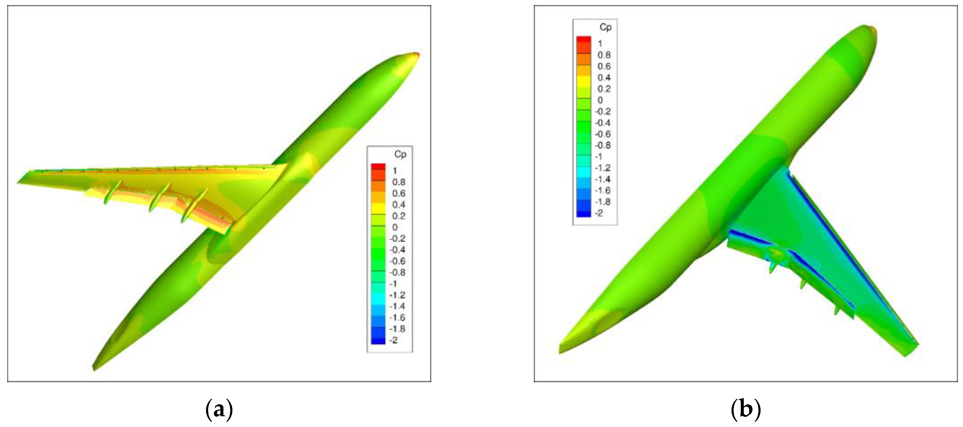
Figure 4 illustrates the distribution of the pressure coefficient across the pressure and suction surfaces of the CRM-HL baseline model. It is evident that the pressure on the pressure surface is notably higher than that on the suction surface. The pressure coefficient reaches its minimum within the slat gap region, primarily attributed to the acceleration of the flow. Conversely, the maximum pressure coefficient is observed on the flap pressure surface of the flap. An analogous pressure distribution was observed on both the pressure and suction surfaces of the CRM-HL modified model.
In the present study, a rigorous comparison is undertaken between the numerically computed surface pressures and the experimental measurements [
49].
Figure 5 illustrates the predefined planar cuts utilized in the experiment setup [
49]. The parameter
, defined as the spanwise direction normalized by the total semispan length, serves as a common reference for this comparison. As evident from the data presented in
Figure 6, the agreement between the experimental data and CFD results is remarkably satisfactory across all the spanwise stations, validating the accuracy of the numerical simulations.
Figure 7 presents a comparative analysis of the surface pressure distribution across eight distinct cuts on the wing, as previously depicted in
Figure 5. This comparison highlights the profound impact of the SGF on the pressure distributions within the slat region. Particularly, the implementation of the SGF significantly reduces the pressure on the slat suction surface, while simultaneously enhancing the pressure on the pressure side. This combined effect is anticipated to contribute to an enhancement in lift within the slat region. Furthermore, the introduction of the SGF is observed to elevate the pressure on the suction side at the main wing’s leading edge, resulting in a reduction of the lift coefficient. Nevertheless, it is noteworthy that the pressure distribution across the flap region remains largely unaffected by the inclusion of the SGF.
Table 1 presents the impact of the SGF on global aerodynamic performance, summarizing lift coefficients, drag coefficients, and lift-to-drag ratio. The results indicate that the SGF device slightly increased the lift coefficient while decreasing the drag coefficient, consequently enhancing the lift-to-drag ratio. These findings offer valuable quantitative evidence for understanding the aerodynamic consequences of the SGF on wing performance.
Figure 8 illustrates a comparison of the velocity magnitude distribution across four distinct cross-sections between the CRM-HL baseline model and the CRM-HL modified model. The CRM-HL baseline model is characterized by low-velocity recirculation within the slat cove and a high-speed gap flow. Similarly, the CRM-HL modified model, incorporating an SGF, exhibits a comparable flow pattern, with a noticeably low-speed recirculation bubble within the slat cove. However, a noticeable difference emerges in the dimension of the low velocity recirculation within the slat cove between the two models. In the CRM-HL baseline model, the length of the low-velocity recirculation is defined as the distance from the slat cusp to the point of the shear layer impingement onto the slat’s pressure surface. Conversely, for the CRM-HL modified model, this length is measured from the slat cusp to the point where the shear layer impinged on the main wing’s pressure surface.
Figure 9 defines the flow field parameters relating to the noise characteristics of the slat, where
L represents the distance between the separation point near the cusp and the reattachment location,
denotes the shear layer length between the slat cusp and the reattachment location, and
is the chord length of the slat. It is evident from
Figure 9 that the length of the low-speed recirculation in the CRM-HL modified model is significantly greater than that in the CRM-HL baseline model. The mean values of
L and
are 0.0608 m and 0.1020 m, respectively, as listed in
Table 2. Additionally, the flow velocity within the slat gap in the CRM-HL baseline model surpasses that of the CRM-HL modified model. Undoubtedly, these differences in the flow field are anticipated to exert a consequential influence on both near-field and far-field noise characteristics. A detailed comparative analysis of the far-field noise between the two models will be conducted in the subsequent section.
3.2. Analysis of the Unsteady Flow Field
It has been revealed that the predominant source of slat noise is dipole sources resulting from surface pressure fluctuations. In this section, we present an analysis of airframe noise sources by examining airframe surface pressure fluctuations.
Figure 10 presents a comparative analysis of the root mean square (RMS) pressure fluctuations on the airframe’s solid surface between the CRM-HL baseline model and the CRM-HL modified model.
Figure 10a,b depicts the comparison from a top view, whereas
Figure 10c,d offers the comparison from a bottom view. In the case of the CRM-HL baseline model, the maximum RMS pressure fluctuations are primarily located at the main wing’s leading edge, the slat pressure surface, and the flap’s suction surface. These phenomena are mainly attributed to the high velocity of the slat gap flow and the unsteady slat cove flow. Conversely, the CRM-HL modified model, equipped with an SGF that eliminates the slat gap, results in the absence of pressure fluctuations on the leading edge of the main wing. This modification would effectively reduce slat noise sources. Furthermore, the RMS pressure fluctuations on the slat pressure surface are increased due to the downward movement of the impingement region of the slat shear layer caused by the SGF.
Figure 11 presents a comparative analysis of the surface
distribution along eight cuts on the wing, as previously illustrated in
Figure 5. Overall, the implementation of the SGF has resulted in a reduction in the
distribution across the wing surfaces. However, a notable exception is observed at cut A, situated proximate to the root of the wing. Here, the SGF slightly increased the
distribution on the suction surface of the slat. Additionally, the SGF has contributed to an increase in the
distributions on the flap surface.
To investigate the distribution of spanwise dipole sources, two distinct spanwise cross-sectional cuts of the wing, as depicted in
Figure 12, were executed. One of these cuts was positioned at the slat trailing edge, while the other cut was situated at the main wing’s leading edge.
Figure 13 presents a comparative analysis of the
distribution along these two spanwise cuts, comparing the CRM-HL baseline model and CRM-HL modified model. The results indicate a significant reduction in pressure fluctuations attributable to the implementation of the SGF. In addition, a noteworthy divergence is observed in the spanwise pressure fluctuation distribution between the CRM-HL baseline model and the CRM-HL modified model. Specifically, for the CRM-HL baseline model, the pressure fluctuations exhibit a relatively uniform distribution across the spanwise dimension. However, in the case of the CRM-HL modified model, the pressure fluctuations are discernibly higher in the wing tip region compared to the wing root, indicating a non-uniform spanwise pressure distribution.
According to the dipole source term in the FW-H equation, the rate of
at the source location is proportional to the far-field part of the dipole noise
. Therefore, a comparative analysis of the distribution of the derivative of the pressure fluctuation between the CRM-HL baseline model and the CRM-HL modified model is presented in
Figure 14. The comparison is depicted from both top and bottom views in
Figure 14a–d. In the case of the CRM-HL baseline model, it is observed that the maximum RMS derivative of pressure fluctuations is predominantly located at the main wing’s leading edge, the slat cove surface, and the suction surface of the flap. This occurrence can be attributed to the high velocity of the slat gap flow and the unsteady slat cove flow. However, the CRM-HL modified model, featuring an SGF, eliminates the slat gap, resulting in the absence of the derivative of the pressure fluctuation on the main wing’s leading edge. Consequently, this leads to a decrease in the slat noise sources. Moreover, the RMS derivative of pressure fluctuations in the CRM-HL modified model’s slat cove surface exhibits a shift towards the outboard region in comparison to the CRM-HL baseline model. This discernible shift is primarily attributed to the spanwise flow occurring from the inboard to the outboard within the slat cove.
Figure 15 presents a comparative analysis of the surface pressure fluctuation rate
distribution across eight distinct cuts on the wing, as initially depicted in
Figure 5. Overall, the incorporation of the SGF has led to a significant reduction in the surface
distribution on both the slat surface and the main wing surfaces. Conversely, the SGF has induced an increase in the
distributions on the flap surface.
Figure 16 conducts a comparative analysis of the surface pressure fluctuation rate
distribution along two spanwise cuts between the CRM-HL baseline model and CRM-HL modified model. The results demonstrate a statistically significant reduction in pressure fluctuations, which can be directly attributed to the implementation of the SGF. Furthermore, a pronounced divergence is observed in the spanwise pressure fluctuation rate distribution between the CRM-HL baseline model and CRM-HL modified model. Specifically, for the CRM-HL baseline model, the
exhibits a relatively uniform distribution across the entire spanwise direction. In contrast, in the case of the CRM-HL modified model, a notable deviation is noted, where the
values are significantly higher in the wing tip region compared to the wing root. This finding indicates a non-uniform spanwise pressure fluctuation rate distribution in the modified model. Given the inherent dipole nature of the airframe noise source, the weakening of these noise sources in the inboard regions in the modified model is anticipated to yield a substantial reduction in the amplitude of the far-field noise. Such weakening in the inboard regions is expected to be effective in minimizing the propagation of noise waves to the far-field region, thereby enhancing the overall noise reduction performance of the modified model.
Figure 17 compares the instantaneous vortical structures between the CRM-HL baseline model and the CRM-HL modified model. Specifically,
Figure 17a,b offers a top-view comparison, while
Figure 17c,d provides a bottom-view comparison. A notable observation is that the vortical structures present on the upper surface of the wing in the baseline model were effectively mitigated by the introduction of the SGF in the modified model. Additionally, the vortexes within the slat cove were weakened and exhibited a shift from the inboard to the outboard direction due to the presence of the SGF. These findings suggest that the SGF plays a pivotal role in modifying the vortical dynamics of the wing, potentially leading to noise reduction.
3.3. Analysis of the Near-Field Noise
The FW-H equation has revealed that the near-field noise source differs from the far-field noise source. Specifically, within the near-field region, pressure fluctuations constitute the primary noise source, whereas in the far-field region, the temporal derivative of the pressure fluctuation emerges as the dominant noise contributor. In this section, we will present a comparative analysis of near-field noise between the CRM-HL baseline model and the CRM-HL modified model.
Figure 18 depicts the comparison of near-field noise at a frequency of 1000 Hz between the CRM-HL baseline model and the CRM-HL modified model. In the CRM-HL baseline model, a conspicuous emission of intense noise is observed originating from the leading-edge slat. However, in the CRM-HL modified model equipped with an SGF, a significantly weaker noise level is recorded, indicating that the slat is no longer the primary source of noise.
Figure 19 compares the near-field noise at a frequency of 3000 Hz between the CRM-HL baseline model and the CRM-HL modified model. In the CRM-HL baseline model, the slat emits intense noise. Conversely, the CRM-HL modified model produces weaker noise, and the slat is no longer the major noise source. For the CRM-HL modified model, the near-field noise mainly comes from the flap. This finding underscores the efficacy of the SGF in mitigating slat noise in the near-field region.
Since the introduction of the POD method [
50,
51] into fluid mechanics in 1967, it has been extensively utilized to extract coherent structures to elucidate the underlying mechanisms of unsteady flow phenomena. Utilizing time-series data of pressure fluctuations, the POD technique decomposes the flow dynamics into a low-dimensional data set. This process facilitates the extraction of dominant mode features, enabling a more profound analysis of the SGF noise reduction mechanisms.
In the study, the simulated pressure field data were employed to derive the dominant modes utilizing the POD method.
Figure 20 depicts the distribution of the eigenvalue corresponding to each mode, clearly indicating a significant and rapid decline in these values. When compared to the CRM-HL baseline model, the modified CRM-HL model exhibited a substantial reduction in the energy associated with each mode.
The first four modes of the two CRM-HL models are illustrated in
Figure 21 and
Figure 22. In the CRM-HL baseline model, the first POD mode, exhibiting the highest energetic profile, is attributed to pressure fluctuations in the impingement zone resulting from the interaction between the shear layer and the slat’s pressure surface. Conversely, the pressure fluctuations in the second POD mode are concentrated primarily in the main wing’s leading-edge, which are intimately linked to the high-velocity slat gap flow. The third and fourth modes reveal that the primary flow characteristics are localized in the slat gap. In the CRM-HL modified model, the first and second POD modes exhibit a concentrated distribution in the vicinity of the impingement zone. Conversely, the third and fourth POD modes are focused predominantly on the downstream region of the shear layer. A comparative analysis reveals that, in contrast to the CRM-HL baseline model, the pressure fluctuations within the modified model exhibit a more widespread distribution. This observation demonstrates that the introduction of the SGF significantly redistributed the flow dynamics and pressure fluctuations, resulting in a notable reduction in the mode energy. This alteration is indicative of the SGF’s effectiveness in regulating the flow field and mitigating slat noise.
3.4. Analysis of the Far-Field Airframe Noise
One of the primary objectives of the present research is to evaluate the efficacy of the SGF in mitigating noise levels on practical aircraft configurations. This section specifically aims to conduct a rigorous assessment of the airframe noise reduction by the SGF. To accurately compute the directivity of the airframe noise, a total of 36 microphones, as illustrated in
Figure 23, were positioned in the vicinity of the CRM-HL model. These microphones are placed at a distance of 10 m from the aircraft’s center, representing the far-field measurement points. The sampling frequency was 50 kHz with a sampling time of 0.08 s. Moreover, the far-field sound pressure data were processed using the pwelch function and divided into eight segments for the power spectrum. A Hanning window was used to handle each data segment with an overlap of 50%.
Figure 24 presents a comparison of the far-field airframe noise spectra between the CRM-HL baseline model and the CRM-HL modified model at four different polar angles. It is evident that the airframe noise spectra exhibit a broadband nature. Specifically,
Figure 24a compares the airframe noise spectra at a polar angle of 0 degrees. The far-field airframe noise spectrum for the CRM-HL modified model is notably lower than that of the CRM-HL baseline model within the high-frequency domain above 1000 Hz. Significantly, the SGF reduces the broadband airframe noise by approximately 10 dB, consistent with previous experimental observations for SGF [
36,
45]. However, at low frequencies, the airframe noise reduction by the SGF is negligible.
A similar pattern is observed in the comparison of the far-field airframe noise at the polar angle of 90 degrees, as shown in
Figure 24b. The SGF reduces the airframe noise by about 10 dB in the high-frequency domain. This trend is also obvious in the comparisons at polar angles of 180 and 270 degrees, as displayed in
Figure 24c,d, respectively. Overall, the analyses indicate that the SGF is an effective noise reduction technology, particularly for middle and high-frequency noise.
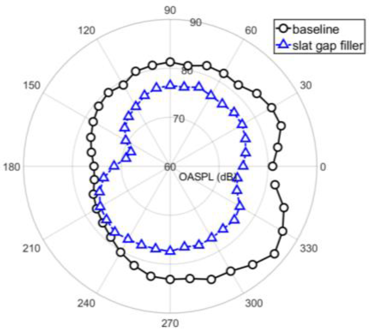
Figure 25 illustrates a comparison of the directivity of the airframe noise level between the CRM-HL baseline model and the CRM-HL modified model. It is evident that the directivity of the CRM-HL baseline model exhibits a dipole characteristic, with the dipole’s orientation being perpendicular to the chord of the main wing. This finding is consistent with airframe noise experiments and theories. In comparison to the CRM-HL baseline model, the CRM-HL modified model demonstrates a significant reduction in airframe noise, particularly at polar angles between 270 degrees and 330 degrees. The maximum noise reduction of approximately 10 dB is achieved at a polar angle of 320 degrees. Furthermore, the noise reduction at a polar angle of 210 degrees is minimal, indicative of a dependency between the polar angle and the effectiveness of noise mitigation.
3.5. Analysis of the Far-Field Slat Noise
The aerodynamic flow across various components of the CRM-HL model is inherently noise-generating, encompassing contributions from slat noise, flap side-edge noise, and others. In this section, we will focus on the pure slat noise. To quantitatively assess the slat noise,
Figure 26 depicts the FW-H integration surface for the leading-edge slat noise in both the CRM-HL baseline and modified models. This integration surface, indicated in blue, encompasses the entire slat surface and the main wing’s leading-edge surface. This comprehensive coverage is necessitated by the substantial contribution of the main wing’s leading-edge surface to the slat noise, stemming from the slat gap flow.
Figure 27 offers a comparative analysis of the far-field slat noise spectra between the CRM-HL baseline model and the CRM-HL modified model across four distinct polar angles. The slat noise spectra exhibit a characteristic broadband nature, with the spectrum for the CRM-HL modified model displaying a significantly lower noise level across the entire frequency domain compared to the CRM-HL baseline model. Furthermore, a notable shift towards lower frequencies is observed in the broadband peak of the slat noise spectra for the CRM-HL modified model when compared to the CRM-HL baseline model. Specifically, the SGF reduces the slat noise by approximately 10 dB within the low-frequency domain and by roughly 20 dB in the high-frequency domain. These trends agree well with the experiment findings [
36]. Overall, these findings underscore the effectiveness of the SGF as a slat noise reduction technology.
3.6. Noise Spectra Scaling for the Slat Gap Filler
Scaling the noise spectra using non-dimensional frequencies is a standard approach to enhance the comprehension of the characteristics of dominant acoustic sources. The Strouhal number is a frequently employed non-dimensional frequency.
Figure 28 exhibits the dependence of the normalized spectral shape on the flow Strouhal number. The spectra of the slat noise source were normalized in terms of amplitude using the overall sound pressure level (OASPL) and in terms of frequency utilizing the Strouhal number, which is based on the mean flow velocity and a characteristic length scale. For the CRM-HL baseline model, the slat chord was employed as the characteristic length scale, defined as
, where
represents the frequency,
is the slat chord length, and
is the mean flow velocity. Conversely, for the CRM-HL modified model, the characteristic length scale was taken as the distance from the slat cusp to the impingement point on the pressure surface of the main wing, formulated as
, where
signifies this distance. Across the entire frequency range, a satisfactory data collapse was observed, indicating a similar characteristic between the slat noise spectra of the CRM-HL baseline model and those of the CRM-HL modified model equipped with a slat gap filler. In addition, the low-frequency spectral shape is proportional to the square of the frequency. The falloff of the spectra is proportional to the inverse square and inverse fourth power of the frequency in the middle- and high-frequency ranges, respectively. The shape of the slat noise spectra agrees well with the experimental measurements [
46,
47]. The revealed scaling laws for the observed slat noise spectra establish a fundamental foundation for the development of a physics-based slat gap filler prediction model.
4. Conclusions
Slat noise reduction during the approach and landing stage is a critical concern in aviation acoustics. SGF technology has shown promise in this regard and has been utilized in commercial aircraft. However, the specific mechanism by which the SGF reduces noise and its noise characteristic remains unclear.
This study aims to numerically investigate the noise reduction achieved by the SGF and to analyze its noise characteristics. The CRM-HL model is used for the computation of aerodynamics and aeroacoustics. The SGF is implemented to mitigate slat noise. The unsteady flow field of the CRM-HL model at AoA of 3 degrees is computed using the LBM solver PowerFLOW, followed by the utilization of the FW-H method to compute far-field noise.
The CFD results obtained for the CRM-HL baseline model demonstrate satisfactory agreement with experimental measurements, validating the numerical approach. Furthermore, the POD technique is employed to elucidate the near-field flow dynamics of the SGF. The result indicates that the incorporation of the SGF device redistributes the flow dynamics and pressure fluctuations, leading to a notable reduction in mode energy. Moreover, it is demonstrated that the SGF can significantly reduce slat noise. The analysis of the noise generation mechanism reveals that the SGF eliminates surface pressure fluctuations on the main wing’s leading edge, and the frequency peak of the SGF’s broadband noise is shifted towards lower frequencies compared to the baseline slotted slat. This shift is primarily attributed to the enlargement of the slat cove flow vortex due to the SGF. Additionally, the spanwise distribution of the slat cove flow noise source is shifted outboard by the SGF, thereby reducing the propagation of far-field noise.
Finally, a rigorous analysis was conducted on the scaling behavior of the slat noise spectra between the CRM-HL baseline model and the CRM-HL modified model. It was observed that the slat noise spectra exhibited excellent collapse when the slat noise spectra were normalized by the OASPL for amplitude scaling and by the Strouhal number, derived from the incoming flow velocity and characteristic length scale, for frequency scaling. The insights gained from this study, particularly the noise reduction mechanism and spectra scaling laws of SGF, will facilitate the development of a physics-based noise prediction model for SGF, which will aid in the optimization and design of noise-mitigating aircraft components.


