Entry Guidance for Hypersonic Glide Vehicles via Two-Phase hp-Adaptive Sequential Convex Programming

Abstract

This paper addresses the real-time trajectory generation problem for hypersonic glide vehicles (HGVs) during atmospheric entry, subject to complex constraints including aerothermal limits, actuator bounds, and no-fly zones (NFZs). To achieve efficient and reliable trajectory planning, a two-phase hp-adaptive sequential convex programming (SCP) framework is proposed. NFZ avoidance is reformulated as a soft objective to enhance feasibility under tight geometric constraints. In Phase I, a shrinking-trust-region strategy progressively tightens the soft trust-region radius by increasing the penalty weight, effectively suppressing linearization errors. A sensitivity-driven mesh refinement method then allocates collocation points based on their contribution to the objective function. Phase II applies residual-based refinement to reduce discretization errors. The resulting reference trajectory is tracked using a linear quadratic regulator (LQR) within a reference-trajectory-tracking guidance (RTTG) architecture. Simulation results demonstrate that the proposed method achieves convergence in only a few iterations, generating high-fidelity trajectories within 2–3 s. Compared to pseudospectral solvers, the method achieves over 12× computational speed-up while maintaining kilometer-level accuracy. Monte Carlo tests under uncertainties confirm a 100% success rate, with all constraints satisfied. These results validate the proposed method’s robustness, efficiency, and suitability for onboard real-time entry guidance in dynamic mission environments.

1. Introduction

As an advanced aerospace system, hypersonic glide vehicles (HGVs) sustain flight at speeds exceeding Mach 5 and exploit near-space atmospheric gliding and maneuvering to achieve superior penetration capability. The entry-flight phase—from booster separation through the onset of the terminal dive—represents the longest and most critical segment of the mission. Therefore, the entry-guidance law is formulated as a closed-loop between guidance commands and the flight trajectory: it must safely transfer the vehicle from the entry interface to the designated target, satisfy all entry-phase constraints, and produce feasible inputs for the attitude-control system. During this phase, the vehicle endures peak aerothermal loads while requiring precise trajectory control under coupled constraints. This operational complexity necessitates guidance algorithms with autonomous trajectory-replanning capabilities and multi-constraint-satisfaction mechanisms to reconcile the competing demands of flight safety, mission flexibility, and terminal accuracy.

Current entry-guidance algorithms fall into two principal categories: reference-trajectory-tracking guidance (RTTG) and predictor-corrector guidance (PCG). In PCG, terminal-state information—obtained either from analytical expressions or via numerical integration of the vehicle dynamics—is used to adjust guidance commands based on deviations from specified terminal constraints, thereby ensuring accurate targeting [1,2]. Analytical PCG uses closed-form solutions to predict terminal states, achieving high computational efficiency; however, the simplifying assumptions required often restrict its applicability [3,4]. Numerical PCG, in contrast, incorporates integrated flight dynamics to improve model fidelity and extend application scope. To alleviate the cost of repeated integration, most numerical PCG schemes split the algorithm into longitudinal and lateral channels, iteratively solving for one guidance parameter per channel [5,6]. Nevertheless, satisfying multiple—and often competing—constraints and objectives further increases both algorithmic complexity and computational cost [7]. RTTG first computes a reference trajectory from the current state to the target and then employs appropriate control laws to track that trajectory. Early RTTG studies generated reference trajectories offline, applying only minor online corrections without full regeneration [8,9]. With advances in onboard computing power, recent research has moved toward fully online reference-trajectory generation to meet real-time entry requirements [10,11]. Moreover, reference trajectories have progressed from two-dimensional profiles to fully three-dimensional and, most recently, to optimally computed trajectories [12,13].

By formulating trajectory planning as an optimal control problem (OCP), one can enforce entry-phase constraints while optimizing performance indices [14,15,16,17,18]. This dual capability of rigorous constraint satisfaction and performance optimization distinguishes OCP-based methods from traditional trajectory-planning approaches. Numerical OCP solvers are classified into two categories: indirect methods—which derive Pontryagin-based necessary conditions but suffer from sensitivity to initial guesses and difficulty handling complex constraints—and direct methods, which transcribe the OCP into a finite-dimensional nonlinear program (NLP) for robust constraint enforcement via mature solvers. Among direct approaches, pseudospectral techniques [16,17,18] attain high-fidelity state/control approximations for offline design but incur prohibitive computational overhead when applied online, owing to high dimensionality and non-convexity.

Convex optimization offers a promising remedy, providing both computational efficiency and convergence guarantees due to its well-structured problem geometry—global optima can be obtained reliably via polynomial-time interior-point or first-order algorithms. Consequently, convex optimization has become a cornerstone of trajectory planning under stringent constraints. A seminal contribution by Acikmese and Ploen [19] applied second-order cone programming (SOCP) to relax non-convex thrust constraints in Mars powered descent, yielding fuel-optimal trajectories with real-time onboard implementability. Their lossless convexification approach [20] ensures equivalence between the convexified and original non-convex problems, thereby preserving optimality. However, the strong nonlinearities and non-convexities inherent in hypersonic entry dynamics preclude direct lossless convexification in many scenarios. To bridge this gap, sequential convex programming (SCP) frameworks iteratively construct and solve convex surrogates of the original OCP by linearizing or convexifying dynamics, constraints, and objectives around a reference trajectory. Early SCP applications focused on convex relaxation of nonlinear and non-convex terms in the flight dynamics, enabling solutions to diverse entry problems, including minimum-time, minimum-heat-load, and maximum-cross-range trajectory optimization [13,21,22,23,24,25]. Recent research has further enhanced SCP performance by improving convergence speed, solution quality, and computational efficiency—key factors for real-time deployment in hypersonic entry guidance systems [26,27,28,29,30,31,32,33,34,35,36].

Current research predominantly models no-fly-zone (NFZ) avoidance as hard path constraints [23,25,27,36], which entails two principal drawbacks. First, trajectories often converge along NFZ boundaries with insufficient safety margins, increasing vulnerability to disturbances and model uncertainties. Second, when geometric or dynamic constraints render full NFZ avoidance infeasible, the resulting infeasible constraints can trigger SCP divergence and prevent trajectory updates. To address these issues, this study reformulates NFZ avoidance as an optimization objective rather than a rigid constraint. Specifically, we jointly optimize angle-of-attack (AOA) and bank-angle commands—in lieu of fixed AOA profiles—to fully exploit vehicle maneuverability while minimizing NFZ penetration risk. By maximizing NFZ-avoidance capability as the primary objective, the formulation enables progressive trajectory refinement: even when full avoidance is infeasible, the optimizer selects trajectories that minimize NFZ penetration depth, which in turn enhances guidance reliability. Nonetheless, our SCP implementation on this reformulated OCP exhibits persistent gaps relative to pseudospectral-method benchmarks. We identify two dominant error sources limiting trajectory fidelity: (i) linearization residuals from successive convex approximations and (ii) discretization errors arising from mesh selection and numerical differentiation schemes. Accordingly, we shift focus from asymptotic optimality toward precision-enhancing strategies—namely, trust-region shrinkage and adaptive mesh refinement—to systematically mitigate these error components.

The performance of SCP frameworks hinges on the design of their trust-region mechanism, which mediates the trade-off between linearization fidelity and convergence speed. Existing implementations adopt one of two paradigms: hard trust regions or soft trust regions. Hard trust regions impose fixed radii on each convex subproblem. Large radii promote rapid progress toward the global optimum but exacerbate linearization error and can destabilize convergence, while small radii curb approximation errors at the expense of very slow progress. Moreover, hard radii often induce oscillatory divergence near the solution [26], necessitating auxiliary stabilization aids—such as virtual controls, line searches, or adaptive radius tuning—to restore convergence [22,27,28,29]. Soft trust regions, by contrast, treat the trust radius as an optimizable variable penalized in the objective function. This approach naturally avoids infeasibility from linearization-induced constraint mismatches and yields more robust convergence. However, soft trust regions can suffer from suboptimal solutions if the initial trajectory guess is poor or the penalty weight is mis-tuned. Recent advances propose high-order soft trust-region formulations to improve both optimality and convergence efficiency [30].

Discretization profoundly impacts both solution accuracy and computational cost in SCP. Many methods typically used uniformly spaced grids with a fixed number of nodes and central-difference approximations [13,21,22,23,24,25,26,28,30]. While adequate for gently varying trajectories, uniform grids incur large errors under rapid state changes. To improve baseline accuracy, researchers have applied hp-schemes—segmenting the trajectory and using high-order polynomial or pseudospectral discretization within each segment [31,32]—and Chebyshev-based fitting for state approximation and differentiation [33]. Although these techniques boost precision, they still rely on a priori choices of node placement and polynomial order, which may not generalize across problem instances and can degrade performance when a finer grid is required. More recent adaptive discretization strategies automatically refine the mesh based on local error indicators [34,35,36]. Zhou et al. [34] adjust node density according to linearization residuals, adding points where errors are large and removing them where errors are small. Zhang et al. [35] adapt both segment counts and polynomial orders using midpoint differential errors and trajectory curvature. These dynamic schemes achieve high accuracy with fewer nodes, striking a balance between precision and efficiency.

In this work, drawing on hp-adaptive pseudospectral methods, we develop a modified SCP algorithm that integrates a soft trust region and a two-stage iteration to decouple linearization and discretization error control. Stage I employs a shrinking-trust-region strategy by progressively increasing the penalty weight on the trust radius within the soft formulation. A low initial weight facilitates rapid convergence toward the optimum, while subsequent weight escalation contracts the trust region to bound linearization errors. Simultaneously, the mesh is adaptively refined based on objective-function sensitivity computed via adjoint equations—concentrating points where the trajectory has the greatest impact on the performance index and avoiding unnecessary refinement elsewhere. Once the trust radius reaches a prescribed minimum—indicating that linearization errors are under control—the algorithm enters Stage II. Here, we fix a high trust-region penalty weight and apply residual-driven mesh refinement to mitigate discretization errors. This two-stage process yields a reference trajectory that meets the predefined accuracy requirements.

This paper develops a two-stage SCP algorithm tailored for NFZ-constrained entry guidance. Our main contributions are as follows:

• Objective reformulation of NFZ avoidance. We replace hard NFZ constraints with a single objective—maximizing NFZ-avoidance capability—thereby ensuring progressive trajectory refinement even when full avoidance is unattainable.
• Soft-trust-region shrinkage. We introduce a dynamic penalty-weight strategy that contracts the trust region, controls linearization errors, and promotes stable convergence.
• Objective-sensitivity-driven mesh refinement. In Stage I, we leverage adjoint-based sensitivity of the performance objective to drive targeted mesh adaptation, avoiding unnecessary refinement in low-impact regions.

The remainder of this article is organized as follows. In Section 2, we formulate the entry-guidance problem with complete constraint modeling. Section 3 describes the convexification and discretization procedures applied to the resulting OCP. In Section 4, we detail the shrinking-trust-region strategy integrated with adaptive mesh-refinement mechanisms. Section 5 validates the proposed framework via numerical simulations and Monte Carlo analyses. Finally, Section 6 summarizes our conclusions and outlines potential directions for future research.

2. Problem Formulation

2.1. Dynamics

The three-dimensional point-mass dynamics of an HGV over a rotating spherical Earth are described by the following nondimensional equations:

$$\dot{r}=V\sin \gamma ,$$

(1)

$$\dot{\theta }={\displaystyle \frac{V\cos \gamma \sin \psi }{r\cos \phi }},$$

(2)

$$\dot{\phi }={\displaystyle \frac{V\cos \gamma \cos \psi }{r}},$$

(3)

$$\dot{V}=-D-\left({\displaystyle \frac{\sin \gamma }{r^2}}\right)+{\omega }^{2}r\cos \phi (\sin \gamma \cos \phi -\cos \gamma \sin \phi \cos \psi ),$$

(4)

$$\dot{\gamma }={\displaystyle \frac{1}{V}}\left[L\cos \sigma +\left(V^2-{\displaystyle \frac{1}{r}}\right)\left({\displaystyle \frac{\cos \gamma }{r}}\right)+2\omega V\cos \phi \sin \psi +{\omega }^{2}r\cos \phi \left(\cos \gamma \cos \phi +\sin \gamma \cos \psi \sin \phi \right)\right],$$

(5)

$$\dot{\psi }={\displaystyle \frac{1}{V}}\left[{\displaystyle \frac{L\sin \sigma }{\cos \gamma }}+{\displaystyle \frac{V^2}{r}}\cos \gamma \sin \psi \tan \phi -2\omega V\left(\tan \gamma \cos \psi \cos \phi -\sin \phi \right)+{\displaystyle \frac{{\omega }^{2}r}{\cos \gamma }}\sin \psi \sin \phi \cos \phi \right],$$

(6)

where the overdot denotes differentiation with respect to nondimensional time t. Here,

• r is the nondimensional radial distance, defined by r = 1 + H, with H the nondimensional altitude.
• θ and φ are longitude and latitude, respectively.
• V is the nondimensional Earth-relative speed.
• γ and ψ are the flight-path angle and heading angle, respectively.
• ω is the nondimensional Earth rotation rate.
• σ is the bank angle.

Figure 1 depicts the definitions of r, θ, φ, V, γ, ψ, and H in the HGV dynamic model.

The nondimensionalization uses the characteristic scales as follows:

$$t\leftarrow {\displaystyle \frac{t_{\mathrm{physical} }}{\sqrt{R_0/g_0}}},\hspace{0.33em}\hspace{0.33em}V\leftarrow {\displaystyle \frac{V_{\mathrm{physical} }}{\sqrt{g_0{R}_0}}},\hspace{0.33em}\hspace{0.33em}r\leftarrow {\displaystyle \frac{r_{\mathrm{physical} }}{R_0}},$$

(7)

where R₀ = 6378 km is Earth’s radius and g₀ = 9.81 m/s² is the gravitational acceleration at sea level.

The nondimensional lift and drag accelerations, scaled by g₀, are as follows:

$$\left\{\begin{array}{l}L=0.5R_0\rho V^2{S}_{\mathrm{ref} }{C}_L/m\hfill \\ D=0.5R_0\rho V^2{S}_{\mathrm{ref} }{C}_D/m\hfill \end{array}\right.,$$

(8)

where m is the vehicle mass, S_ref the reference area, and C_L, C_D the lift and drag coefficients, which depend on AOA α and Mach number.

The atmospheric density ρ follows an exponential model:

$$\rho ={\rho }_0{\mathrm{e}}^{-H/H_0},$$

(9)

with ρ₀ = 1.225 kg/m³ the sea-level density and H₀ = 1.12 × 10⁻³ the nondimensional scale height.

2.2. Control Variable Selection

To fully exploit HGV maneuverability, we select the AOA α and bank angle σ as the primary control inputs. To prevent physically unrealistic instantaneous changes, we introduce first-order rate constraints by defining new control inputs u₁ and u₂ such that

$$\dot{\alpha }=u_1,\hspace{0.33em}\hspace{0.33em}\hspace{0.33em}\dot{\sigma }=u_2,$$

(10)

with

$$u_{\min }\le u\le u_{\max },$$

(11)

where u_min and u_max are actuator-imposed bounds.

By promoting α and σ to state variables, the state vector expands from six to eight dimensions—x = [r, θ, φ, V, γ, ψ, α, σ]^T—and the control vector becomes u = [u₁, u₂]^T. This state augmentation decouples the vehicle’s trajectory dynamics from actuator dynamics, thereby suppressing high-frequency control oscillations during the SCP iterations [23].

The extended state-space model can then be written compactly as follows:

$$\dot{x}=f(x)+Bu+f_{\omega }(x),$$

(12)

where f(x) and B capture the original point-mass and actuator dynamics, respectively, and f_ω(x) accounts for Coriolis and centrifugal perturbations due to Earth’s rotation (with a normalized rate ω ∼ 10⁻²). Specifically, these three items are given by

$$f(x)=\left[\begin{array}{c}V\sin \gamma \\ V\cos \gamma \sin \psi /(r\cos \phi )\\ V\cos \gamma \cos \psi /r\\ -D-\sin \gamma /r^2\\ L\cos \sigma /V+\left(V^2-1/r\right)\cos \gamma /(Vr)\\ L\sin \sigma /(V\cos \gamma )+V\cos \gamma \sin \psi \tan \phi /r\\ 0\\ 0\end{array}\right],$$

(13)

$$B={\left[\begin{array}{llllllll}0\hfill & 0\hfill & 0\hfill & 0\hfill & 0\hfill & 0\hfill & 1\hfill & 0\hfill \\ 0\hfill & 0\hfill & 0\hfill & 0\hfill & 0\hfill & 0\hfill & 0\hfill & 1\hfill \end{array}\right]}^{\mathrm{T}},$$

(14)

$$f_{\omega }(x)=\left[\begin{array}{c}0\\ 0\\ 0\\ 2\omega \cos \phi \sin \psi +{\displaystyle \frac{{\omega }^{2}r\cos \phi }{V}}(\cos \gamma \cos \phi +\sin \gamma \cos \psi \sin \phi )\\ {\omega }^{2}r\cos \phi (\sin \gamma \cos \phi -\cos \gamma \sin \phi \cos \psi )\\ -2\omega (\tan \gamma \cos \psi \cos \phi -\sin \phi )+{\displaystyle \frac{{\omega }^{2}r\sin \psi \sin \phi \cos \phi }{V\cos \gamma }}\\ 0\\ 0\end{array}\right].$$

(15)

2.3. Optimal Control Problem

We formulate the entry-trajectory optimization as a non-convex optimal control problem over the time interval t ∈ [t₀, t_f], where t₀ = 0 and t_f is mission-specified. The boundary conditions enforce

$$x(t_0)=x_0,\hspace{0.33em}\hspace{0.33em}x(t_f)=x_f,$$

(16)

with x₀ and x_f being the prescribed initial and terminal states, respectively.

Path constraints include limits on heating rate $\dot{Q}$, dynamic pressure q, and load factor n:

$$\dot{Q}=k_Q{\sqrt{R_0{g}_0}}^{3.15}{\rho }^{0.5}{V}^{3.15}\le {\dot{Q}}_{\max },$$

(17)

$$q=0.5R_0{g}_0\rho V^2\le q_{\max },$$

(18)

$$n=\sqrt{L^2+D^2}\le n_{\max },$$

(19)

where k_Q is a constant for the computation of the heating rate. State bounds are enforced by

$$x_{\min }\le x\le x_{\max }.$$

(20)

We model each NFZ as a vertical cylinder centered at longitude θ_N,i and latitude φ_N,i, with radius R_N,i, for i = 1, …, n_N. Defining

$$d_i(x)=\sqrt{{(\theta -{\theta }_{Ni})}^2+{(\phi -{\phi }_{Ni})}^2}$$

(21)

as the great-circle distance from the vehicle to the ith NFZ center, the NFZ-avoidance constraint becomes

$$d_i(x)\ge R_{N,i}.$$

(22)

However, to ensure solver feasibility even when strict avoidance is impossible, we define the instantaneous clearance margin

$$b_i(x)=d_i(x)-R_{N,i},$$

(23)

where b_i(x) < 0 indicates intrusion into NFZ i. The worst-case clearance across all NFZs is as follows:

$$\overline{b}={\min }_{i=1,\dots ,nN}{b}_i(x),$$

(24)

which we seek to maximize. Accordingly, we pose the NFZ-avoidance term in the performance index:

$$J_0=-\overline{b}+{\displaystyle {\int }_{t_0}^{t_f}\left(C_1{u}_1^2(t)+C_2{u}_2^2(t)\right)} \mathrm{d}t.$$

(25)

The first term maximizes the minimum NFZ clearance, while the integral terms penalize rapid control-rate changes to promote smooth α and σ profiles. Correspondingly, the NFZ-avoidance constraint Equation (22) is transformed into

$$d_i(x)\ge \overline{b}+R_{N,i}.$$

(26)

The resulting non-convex optimal control problem P0 is therefore

$$\begin{array}{ll}\min & J_0=-\overline{b}+{\displaystyle {\int }_{t_0}^{t_f}\left(C_1{u}_1^2(t)+C_2{u}_2^2(t)\right)} \mathrm{d}t, \\ \mathrm{s}.\mathrm{t}. & \dot{x}=f(x)+Bu+f_{\omega }(x),\\ & x\left(t_0\right)=x_0,\hspace{0.33em}\hspace{0.33em}x\left(t_f\right)=x_f,\\ & \dot{Q}\le {\dot{Q}}_{\max },\hspace{0.33em}\hspace{0.33em}q\le q_{\max },\hspace{0.33em}\hspace{0.33em}\hspace{0.33em}n\le n_{\max },\\ & x_{\min }\le x\le x_{\max },\hspace{0.33em}\hspace{0.33em}{u}_{\min }\le u\le u_{\max },\\ & d_i(x)\ge \overline{b}+R_{N,i}.\end{array}$$

(27)

This formulation balances NFZ avoidance with actuator effort and discourages trajectories that skirt NFZ boundaries, yielding paths that maximize clearance from all zones. Moreover, when full avoidance of every NFZ is infeasible, the solver still converges to the trajectory that minimizes the worst-case intrusion risk.

3. Convexification and Discretization

3.1. Convexification

The original problem, P0, is non-convex due to the nonlinear vehicle dynamics, path constraints, and NFZ conditions. To obtain a convex approximation at iteration k, we apply successive linearization to the dynamics and logarithmic or Taylor-based reformulations of the path and NFZ constraints.

3.1.1. Dynamics Linearization

We expand the nonlinear dynamics $\dot{x}=f(x)+Bu+f_{\omega }(x)$ about the previous iterate x^k−1 via a first-order Taylor series:

$$\dot{x}\approx f\left(x^{k-1}\right)+A\left(x^{k-1}\right)\left(x-x^{k-1}\right)+Bu+f_{\omega }\left(x^{k-1}\right),$$

(28)

where

$$A(x^{k-1})={\left.{\displaystyle \frac{\partial f(x)}{\partial x}}\right|}_{x=x^{k-1}}=\left[\begin{array}{cccccccc}0& 0& 0& a_{14}& a_{15}& 0& 0& 0\\ a_{21}& 0& a_{23}& a_{24}& a_{25}& a_{26}& 0& 0\\ a_{31}& 0& 0& a_{34}& a_{35}& a_{36}& 0& 0\\ a_{41}& 0& 0& a_{44}& a_{45}& 0& a_{47}& 0\\ a_{51}& 0& 0& a_{54}& a_{55}& 0& a_{57}& a_{58}\\ a_{61}& 0& a_{63}& a_{64}& a_{65}& a_{66}& a_{67}& a_{68}\\ 0& 0& 0& 0& 0& 0& 0& 0\\ 0& 0& 0& 0& 0& 0& 0& 0\end{array}\right]$$

(29)

is the Jacobian of f(x). The Jacobian entries a_ij are given by the partial derivatives of the right-hand side f(x) with respect to each state variable, evaluated at x^k−1. For notational simplicity, we henceforth drop the superscript “(·)^k−1”. The nonzero coefficients are then listed below in compact form:

$$\begin{array}{l}{a}_{14}=\sin \gamma ,\hspace{0.33em}{a}_{15}=V\cos \gamma ,\hspace{0.33em}{a}_{21}=-{\displaystyle \frac{V\cos \gamma \sin \psi }{r^2\cos \phi }},\hspace{0.33em}{a}_{23}={\displaystyle \frac{V\cos \gamma \sin \psi \sin \phi }{r{\cos }^2\phi }},\\ a_{24}={\displaystyle \frac{\cos \gamma \sin \psi }{r\cos \phi }},\hspace{0.33em}{a}_{25}=-{\displaystyle \frac{V\sin \gamma \sin \psi }{r\cos \phi }},\hspace{0.33em}{a}_{26}={\displaystyle \frac{V\cos \gamma \cos \psi }{r\cos \phi }},\hspace{0.33em}{a}_{31}=-{\displaystyle \frac{V\cos \gamma \cos \psi }{r^2}},\\ a_{34}={\displaystyle \frac{\cos \gamma \cos \psi }{r}},\hspace{0.33em}{a}_{35}=-{\displaystyle \frac{V\sin \gamma \cos \psi }{r}},\hspace{0.33em}{a}_{36}=-{\displaystyle \frac{V\cos \gamma \sin \psi }{r}},\hspace{0.33em}{a}_{41}=-D_r+{\displaystyle \frac{2\sin \gamma }{r^3}},\\ a_{44}=-D_V,\hspace{0.33em}{a}_{45}=-{\displaystyle \frac{\cos \gamma }{r^2}},\hspace{0.33em}{a}_{47}=-D_{\alpha },\hspace{0.33em}{a}_{51}={\displaystyle \frac{\cos \sigma }{V}}{L}_r-{\displaystyle \frac{V\cos \gamma }{r^2}}+{\displaystyle \frac{2\cos \gamma }{r^{3}V}},\\ a_{54}={\displaystyle \frac{\cos \sigma }{V}}{L}_V-{\displaystyle \frac{L\cos \sigma }{V^2}}+{\displaystyle \frac{\cos \gamma }{r}}+{\displaystyle \frac{\cos \gamma }{r^2{V}^2}},\hspace{0.33em}{a}_{55}=\left({\displaystyle \frac{1}{r^{2}V}}-{\displaystyle \frac{V}{r}}\right)\sin \gamma ,\hspace{0.33em}{a}_{57}={\displaystyle \frac{L_{\alpha }\cos \sigma }{V}},\\ a_{58}=-{\displaystyle \frac{L\sin \sigma }{V}},\hspace{0.33em}{a}_{61}={\displaystyle \frac{\sin \sigma }{V\cos \gamma }}{L}_r-{\displaystyle \frac{V\cos \gamma \sin \psi \tan \phi }{r^2}},\hspace{0.33em}{a}_{63}={\displaystyle \frac{V\cos \gamma \sin \psi }{r{\cos }^2\phi }},\\ a_{64}={\displaystyle \frac{\sin \sigma }{V\cos \gamma }}{L}_V-{\displaystyle \frac{L\sin \sigma }{V^2\cos \gamma }}+{\displaystyle \frac{\cos \gamma \sin \psi \tan \phi }{r}},\hspace{0.33em}{a}_{65}={\displaystyle \frac{L\sin \sigma \sin \gamma }{V{\cos }^2\gamma }}-{\displaystyle \frac{V\sin \gamma \sin \psi \tan \phi }{r}},\\ a_{66}={\displaystyle \frac{V\cos \gamma \cos \psi \tan \phi }{r}},\hspace{0.33em}{a}_{67}={\displaystyle \frac{L_{\alpha }\sin \sigma }{V\cos \gamma }},\hspace{0.33em}{a}_{68}={\displaystyle \frac{L\cos \sigma }{V\cos \gamma }},\\ D_r={\displaystyle \frac{\partial D}{\partial r}}=-{\displaystyle \frac{R_0}{H_0}}D,\hspace{0.33em}{D}_V={\displaystyle \frac{\partial D}{\partial V}}={\displaystyle \frac{2D}{V}},\hspace{0.33em}{D}_{\alpha }={\displaystyle \frac{\partial D}{\partial \alpha }}={\displaystyle \frac{D}{C_D}}{\displaystyle \frac{\partial C_D}{\partial \alpha }},\\ L_r={\displaystyle \frac{\partial L}{\partial r}}=-{\displaystyle \frac{R_0}{H_0}}L,\hspace{0.33em}{L}_V={\displaystyle \frac{\partial L}{\partial V}}={\displaystyle \frac{2L}{V}},\hspace{0.33em}{L}_{\alpha }={\displaystyle \frac{\partial L}{\partial \alpha }}={\displaystyle \frac{L}{C_L}}{\displaystyle \frac{\partial C_L}{\partial \alpha }}.\end{array}$$

Terms in f_ω(x) are similarly frozen at x^k−1, since their contribution is $𝒪$(ω) ≪ 1. A component-wise trust-region constraint

$$\left|x-x^{k-1}\right|\le {\delta }_{\mathrm{hard}}$$

(30)

is imposed to bound the linearization error, with δ_hard ∈ ℝ⁸ defining per-state radii.

3.1.2. Path-Constraint Convexification

The heating rate, dynamic pressure, and load factor constraints depend nonlinearly on (r, V), yielding a non-convex feasible region. Earlier, Reference [23] introduced the vehicle’s total mechanical energy as an auxiliary variable, which converts heating and pressure limits into affine bounds on r; however, that energy-based reformulation cannot enforce load-factor limits unless an AOA profile is specified in advance. To overcome these shortcomings without fixing α(t), we instead apply the logarithmic transformations of Reference [27]:

$$p_1(x)\triangleq \ln (\dot{Q})=\ln \left(k_Q{\sqrt{R_0{g}_0}}^{3.15}{\rho }_0^{0.5}\right)-{\displaystyle \frac{H}{2H_0}}+3.15\ln V-\ln {\dot{Q}}_{\max }\le 0,$$

(31)

$$p_2(x)\triangleq \ln (q)=\ln \left(0.5R_0{g}_0{\rho }_0\right)-{\displaystyle \frac{H}{H_0}}+2\ln V-\ln q_{\max }\le 0,$$

(32)

$$p_3(x)\triangleq \ln (n)=\ln \left({\displaystyle \frac{R_0{\rho }_0{S}_{\mathrm{ref} }}{2m}}\right)-{\displaystyle \frac{H}{H_0}}+2\ln V+0.5\ln \left(C_L^2+C_D^2\right)-\ln n_{\max }\le 0,$$

(33)

which convert upper-bound inequalities into convex constraints. Each p_i(x) is then linearized at x^k−1:

$$p_i\left(x^{k-1}\right)+\nabla p_i{\left(x^{k-1}\right)}^{\mathrm{T}}\left(x-x^{k-1}\right)\le 0,\hspace{0.33em}\hspace{0.33em}\hspace{0.33em}i=1,2,3.$$

(34)

3.1.3. NFZ-Constraint Convexification

To facilitate linearization, we square both sides of Equation (26) to obtain the equivalent quadratic form:

$$z_i(x)\triangleq {(\theta -{\theta }_{Ni})}^2+{(\phi -{\phi }_{Ni})}^2\ge {(\overline{b}+R_{N,i})}^2.$$

(35)

The constraint function z_i(x) is then linearized around the previous iteration’s solution x^k−1 as follows:

$$z_i\left(x^{k-1}\right)+\nabla z_i{\left(x^{k-1}\right)}^{\mathrm{T}}\left(x-x^{k-1}\right)\ge \widehat{b},\hspace{0.33em}i=1,\dots ,n_N,$$

(36)

where $\widehat{b}$ is an auxiliary slack variable satisfying

$$\widehat{b}\ge {(\overline{b}+R_{N,i})}^2.$$

(37)

To maintain consistency in the convex formulation, the worst-case clearance $\overline{b}$ in the objective function is also replaced by the slack variable $\widehat{b}$.

3.1.4. Objective Reformulation

To embed control-effort penalties into a convex framework, we introduce slack variables η₁ and η₂ and enforce

$$u_1^2\le {\eta }_1,\hspace{0.33em}{u}_2^2\le {\eta }_2.$$

(38)

The cost becomes

$$J_1=-\widehat{b}+{\displaystyle {\int }_{t_0}^{t_f}\left(C_1{\eta }_1+C_2{\eta }_2\right)} \mathrm{d}t,$$

(39)

which is second-order-cone representable.

Combining these steps yields the convex subproblem P1, parameterized by x^k−1:

$$\begin{array}{ll}\min & J_1=-\widehat{b}+{\displaystyle {\int }_{t_0}^{t_f}\left(C_1{\eta }_1+C_2{\eta }_2\right)} \mathrm{d}t, \\ \mathrm{s}.\mathrm{t}. & \dot{x}=f\left(x^{k-1}\right)+A\left(x^{k-1}\right)\left(x-x^{k-1}\right)+Bu+f_{\omega }\left(x^{k-1}\right),\\ & \left|x-x^{k-1}\right|\le {\delta }_{\mathrm{hard}},\hspace{0.33em}\hspace{0.33em}x\left(t_0\right)=x_0,\hspace{0.33em}\hspace{0.33em}x\left(t_f\right)=x_f,\\ & x_{\min }\le x\le x_{\max },\hspace{0.33em}\hspace{0.33em}{u}_{\min }\le u\le u_{\max }\\ & p_i\left(x^{k-1}\right)+\nabla p_i{\left(x^{k-1}\right)}^{\mathrm{T}}\left(x-x^{k-1}\right)\le 0,\hspace{0.33em}i=1,2,3, \\ & z_i\left(x^{k-1}\right)+\nabla z_i{\left(x^{k-1}\right)}^{\mathrm{T}}\left(x-x^{k-1}\right)\ge 0,\hspace{0.33em}i=1,\dots ,n_N,\\ & u_1^2\le {\eta }_1,\hspace{0.33em}\hspace{0.33em}{u}_2^2\le {\eta }_2.\end{array}$$

(40)

3.2. Discretization and Approximation

To solve the convex subproblem P1 numerically, we employ an hp-adaptive Radau pseudospectral scheme, which achieves higher accuracy per node than trapezoidal rules under comparable grid densities.

First, we partition the original time domain [t₀, t_f] into Y mesh intervals [t_y−1, t_y] (y = 1, …, Y), with mesh points t₀ < t₁ < … < t_Y = t_f. Each subinterval is mapped to the domain τ ∈ [−1, +1] via the affine transform

$$\tau ={\displaystyle \frac{2t-\left(t_y+t_{y-1}\right)}{t_y-t_{y-1}}}.$$

(41)

Within each interval, we approximate the state trajectory x^(y)(τ) by a degree-N_y Lagrange interpolant on the Legendre-Gauss-Radau (LGR) nodes ${\left\{{\tau }_i^{(y)}\right\}}_{i=1}^{Ny}$ plus the terminal point ${\tau }_{N_y+1}^{(y)}=+1$:

$$x^{(y)}(\tau )\approx X^{(y)}(\tau )={\displaystyle {\displaystyle \sum _{i=1}^{N_y+1}}{X}_i^{(y)}}{L}_i^{(y)}(\tau ),\hspace{1em}\hspace{1em}{L}_i^{(y)}(\tau )={\displaystyle {\displaystyle \prod _{\begin{array}{c}j=1\\ j\ne i\end{array}}^{N_y+1}}\frac{\tau -{\tau }_j^{(y)}}{{\tau }_i^{(y)}-{\tau }_j^{(y)}}},$$

(42)

where $L_i^{(y)}(\tau )$ denotes the Lagrange basis polynomial. Controls u^(y)(τ) are likewise interpolated at the N_y LGR points:

$$u^{(y)}(\tau )\approx U^{(y)}(\tau )={\displaystyle {\displaystyle \sum _{i=1}^{N_y}}{U}_i^{(y)}}{\tilde{L}}_i^{(y)}(\tau ),\hspace{1em}\hspace{1em}{\tilde{L}}_i^{(y)}(\tau )={\displaystyle {\displaystyle \prod _{\begin{array}{c}j=1\\ j\ne i\end{array}}^{N_y}}\frac{\tau -{\tau }_j^{(y)}}{{\tau }_i^{(y)}-{\tau }_j^{(y)}}}.$$

(43)

The cost functional is approximated by composite LGR quadrature:

$$J_2\approx -\widehat{b}+{\displaystyle {\displaystyle \sum _{y=1}^Y}{\displaystyle {\displaystyle \sum _{i=1}^{N_y}}\frac{t_y-t_{y-1}}{2}}}{w}_i^{(y)}\left(C_1{\eta }_{1,i}^{(y)}+C_2{\eta }_{2,i}^{(y)}\right),$$

(44)

where $w_i^{(y)}$ are the LGR weights on interval y.

Dynamic constraints are enforced at each collocation point via the implicit Radau collocation relation [37]:

$$X_{i+1}^{(y)}-X_1^{(y)}-{\displaystyle \frac{t_y-t_{y-1}}{2}}{\displaystyle {\displaystyle \sum _{j=1}^{N_y}}{I}_{ij}^{(y)}}\left[f\left(X_j^{(y)(k-1)}\right)+A\left(X_j^{(y)(k-1)}\right)\left(X_j^{(y)}-X_j^{(y)(k-1)}\right)+B{U}_j^{(y)}+f_{\omega }\left(X_j^{(y)(k-1)}\right)\right]=\mathbf{0},$$

(45)

for i = 1,…,N_y and y = 1,…Y. Here, $X_1^{(y)}$ represents the state at τ = −1, and I^(y) ∈ ℝ^Ny×Ny is the Radau integration matrix obtained from the LGR differentiation matrix D^(y):

$$D_{ij}^{(y)}={\left[{\displaystyle \frac{\mathrm{d}{\mathcal{l}}_j^{(y)}(\tau )}{\mathrm{d}\tau }}\right]}_{{\tau }_i^{(y)}},\hspace{1em}{I}^{(y)}={\left[D_{2:N_k+1}^{(y)}\right]}^{-1}.$$

(46)

All path and NFZ constraints are collocated similarly, e.g.,

$$p_j\left(X_i^{(y)(k-1)}\right)+\nabla p_j{\left(X_i^{(y)(k-1)}\right)}^{\mathrm{T}}\left(X_i^{(y)}-X_i^{(y)(k-1)}\right)\le 0,$$

(47)

$$z_j\left(X_i^{(y)(k-1)}\right)+\nabla z_j{\left(X_i^{(y)(k-1)}\right)}^{\mathrm{T}}\left(X_i^{(y)}-X_i^{(y)(k-1)}\right)\ge 0.$$

(48)

Throughout, y = 1, …, Y indexes mesh intervals, and i = 1, …, N_y + 1 indexes collocation points. Other constraints (e.g., boundary, trust-region, control bounds, and auxiliary variables) are discretized in an analogous fashion and are omitted here for brevity.

The discrete SCP subproblem, denoted P2, can be written explicitly as follows. We collect all interval and collocation indices y = 1, …, Y, i = 1, …, N_y (and i = N_y + 1 for terminal-point constraints) and define the decision variables.

$$\left\{X_i^{(y)},U_i^{(y)},{\eta }_{1,i}^{(y)},{\eta }_{2,i}^{(y)}\right\} \mathrm{for} i=1,\dots ,N_y+1,y=1,\dots ,Y,$$

together with the worst-case clearance $\widehat{b}$. Then

$$\begin{array}{ll}\min J_2& \approx -\widehat{b}+{\displaystyle {\displaystyle \sum _{y=1}^Y}{\displaystyle {\displaystyle \sum _{i=1}^{N_y}}\frac{t_y-t_{y-1}}{2}}}{w}_i^{(y)}\left(C_1{\eta }_{1,i}^{(y)}+C_2{\eta }_{2,i}^{(y)}\right), \\ \mathrm{s}.\mathrm{t}. & X_{i+1}^{(y)}-X_1^{(y)}-{\displaystyle \frac{t_y-t_{y-1}}{2}}{\displaystyle {\displaystyle \sum _{j=1}^{N_y}}{I}_{ij}^{(y)}}\left[f\left(X_j^{(y)(k-1)}\right)+A\left(X_j^{(y)(k-1)}\right)\left(X_j^{(y)}-X_j^{(y)(k-1)}\right)+B{U}_j^{(y)}+f_{\omega }\left(X_j^{(y)(k-1)}\right)\right]=\mathbf{0},\\ & i=1,\dots ,N_y,\hspace{0.33em}\hspace{0.33em}y=1,\dots ,Y,\\ & X_1^{(1)}=x_0,\hspace{0.33em}\hspace{0.33em}{X}_{NY+1}^{(Y)}=x_f,\\ & x_{\min }\le X_i^{(y)}\le x_{\max },\hspace{0.33em}\hspace{0.33em}{u}_{\min }\le U_i^{(y)}\le u_{\max },\hspace{0.33em}\hspace{0.33em}\left|X_i^{(y)}-X_i^{(y)(k-1)}\right|\le {\delta }_{\mathrm{hard}},\hspace{0.33em}\hspace{0.33em}i=1,\dots ,N_y+1,\hspace{0.33em}\hspace{0.33em}y=1,\dots ,Y,\\ & p_j\left(X_i^{(y)(k-1)}\right)+\nabla p_j{\left(X_i^{(y)(k-1)}\right)}^{\mathrm{T}}\left(X_i^{(y)}-X_i^{(y)(k-1)}\right)\le 0,\hspace{0.33em}\hspace{0.33em}j=1,2,3,\hspace{0.33em}\hspace{0.33em}i=1,\dots ,N_y+1,\hspace{0.33em}\hspace{0.33em}\hspace{0.33em}y=1,\dots ,Y,\\ & z_j\left(X_i^{(y)(k-1)}\right)+\nabla z_j{\left(X_i^{(y)(k-1)}\right)}^{\mathrm{T}}\left(X_i^{(y)}-X_i^{(y)(k-1)}\right)\ge 0,\hspace{0.33em}\hspace{0.33em}j=1,\dots ,n_N,\hspace{0.33em}\hspace{0.33em}i=1,\dots ,N_y+1,\hspace{0.33em}\hspace{0.33em}y=1,\dots ,Y,\\ & U_i^{(y)2}\le {\eta }_{1,i}^{(y)},\hspace{0.33em}\hspace{0.33em}{U}_i^{(y)2}\le {\eta }_{2,i}^{(y)},\hspace{0.33em}\hspace{0.33em}i=1,\dots ,N_y,\hspace{0.33em}\hspace{0.33em}y=1,\dots ,Y.\end{array}$$

(49)

Solving this convex program for each SCP iteration k produces the updated state and control trajectories for the next linearization.

4. Entry Guidance Method

The gap between the SCP-generated reference trajectory and the trajectory obtained by forward-integrating the nominal vehicle dynamics under the optimized control inputs arises from two sources: (i) linearization error introduced during convexification and (ii) discretization error from the pseudospectral approximation. To address these errors, our entry-guidance method first refines the reference via a two-phase trust-region scheme coupled with hp-adaptive mesh refinement. Once a high-accuracy reference is available, we employ an online RTTG law to command the vehicle to follow the optimized path in real time.

4.1. Shrinking-Trust-Region Strategy

During the initial SCP iterations or when updating the reference trajectory to accommodate new mission requirements, we must balance rapid convergence against the linearization errors introduced by first-order Taylor expansions. To increase flexibility, we relax the hard trust-region constraint in Equation (30) into a first-order soft trust region:

$${‖X_i^{(y)}-X_i^{(y)(k-1)}‖}_2\le {\delta }_{\mathrm{soft},i}^{(y)}, i=1,\dots ,N_y,y=1,\dots ,Y,$$

(50)

where δ_soft collects all per-point soft radii. We then penalize any trust-region violation by adding a weighted norm of δ_soft to the cost. The modified objective becomes

$$J_3=-\widehat{b}+{\displaystyle {\displaystyle \sum _{y=1}^Y}{\displaystyle {\displaystyle \sum _{i=1}^{N_y}}\frac{t_y-t_{y-1}}{2}}}{w}_i^{(y)}\left(C_1{\eta }_{1,i}^{(y)}+C_2{\eta }_{2,i}^{(y)}\right)+C_3{‖{\delta }_{\mathrm{soft}}‖}_2.$$

(51)

Accordingly, P3 (Soft-Trust-Region SCP) is formulated as follows:

$$\begin{array}{ll}\min & J_3=-\widehat{b}+{\displaystyle {\displaystyle \sum _{y=1}^Y}{\displaystyle {\displaystyle \sum _{i=1}^{N_y}}\frac{t_y-t_{y-1}}{2}}}{w}_i^{(y)}\left(C_1{\eta }_{1,i}^{(y)}+C_2{\eta }_{2,i}^{(y)}\right)+C_3{‖{\delta }_{\mathrm{soft}}‖}_2, \\ \mathrm{s}.\mathrm{t}. & {‖X_i^{(y)}-X_i^{(y)(k-1)}‖}_2\le {\delta }_{\mathrm{soft},i}^{(y)}, i=1,\dots ,N_y,y=1,\dots ,Y,\\ & \mathrm{All} \mathrm{other} \mathrm{convexified} \mathrm{constraints} \mathrm{from} \mathrm{P}2.\end{array}$$

(52)

By tuning the penalty weight C₃, the solver naturally contracts the trust region as needed—achieving a compromise between global convergence speed and local linearization accuracy.

To construct a higher-order soft trust region (taking the fourth order as an example), we introduce two tiers of auxiliary variables, $d_{1,i}^{(y)}$ and $d_{2,i}^{(y)}$, that penalize increasingly larger deviations. Specifically, for each collocation point i in interval y, we enforce the following:

$$d_{1,i}^{(y)}\ge {\left({\delta }_{\mathrm{soft},i}^{(y)}\right)}^2,\hspace{0.33em}\hspace{0.33em}\hspace{0.33em}{d}_{2,i}^{(y)}\ge {\left(d_{1,i}^{(y)}\right)}^2,$$

(53)

and replace the trust-region penalty in the cost by the 2-norm of the highest-order variables:

$$J_4=-\widehat{b}+{\displaystyle {\displaystyle \sum _{y=1}^Y}{\displaystyle {\displaystyle \sum _{i=1}^{N_y}}\frac{t_y-t_{y-1}}{2}}}{w}_i^{(y)}\left(C_1{\eta }_{1,i}^{(y)}+C_2{\eta }_{2,i}^{(y)}\right)+C_3{‖d_2‖}_2.$$

(54)

Accordingly, the fourth-order soft trust-region subproblem P4 is

$$\begin{array}{ll}\min & J_4=-\widehat{b}+{\displaystyle {\displaystyle \sum _{y=1}^Y}{\displaystyle {\displaystyle \sum _{i=1}^{N_y}}\frac{t_y-t_{y-1}}{2}}}{w}_i^{(y)}\left(C_1{\eta }_{1,i}^{(y)}+C_2{\eta }_{2,i}^{(y)}\right)+C_3{‖d_2‖}_2, \\ \mathrm{s}.\mathrm{t}.& \mathrm{All} \mathrm{condtraints} \mathrm{from} \mathrm{P}3,\\ & d_{1,i}^{(y)}\ge {\left({\delta }_{\mathrm{soft},i}^{(y)}\right)}^2,\hspace{0.33em}\hspace{0.33em}\hspace{0.33em}{d}_{2,i}^{(y)}\ge {\left(d_{1,i}^{(y)}\right)}^2,i=1,\dots ,N_y,y=1,\dots ,Y.\end{array}$$

(55)

By penalizing $‖d_2‖$, the solver discourages large trust-region violations even more strongly while retaining convexity via second-order-cone representations of the quadratic inequalities.

Ideally, a soft trust region permits larger deviations during early SCP iterations—facilitating rapid convergence toward the optimal solution—and gradually contracts in later stages due to the influence of the penalty term, thereby suppressing oscillatory behavior and avoiding infeasibility caused by excessive linearization error. However, practical application to the current problem reveals that a fixed penalty weight C₃ hinders this ideal behavior. Specifically, a small C₃ leads to convergence toward a relatively large average trust-region radius, while a large C₃ forces the solution to remain overly conservative, potentially stalling progress.

To address this, we initialize C₃ with a small value and increase it multiplicatively by a factor k₃ > 1 after each iteration, up to a prescribed maximum C_3,max,. This adaptive update scheme is referred to as the Shrinking-Trust-Region Strategy, and it constitutes Phase I of the overall guidance method. Phase I terminates once the average trust-region radius satisfies the convergence criterion.

$${\displaystyle \frac{{‖{\delta }_{\mathrm{soft} }‖}_2}{1+{\displaystyle {\sum }_{y=1}^Y{N}_y}}}\le {\epsilon }_{\delta }.$$

(56)

The progressive increase in penalty weight compels the solver to shift emphasis from objective minimization toward enforcing trust-region bounds, effectively reducing the average deviation across all discretization points—that is, including both collocation nodes and terminal points—with a total count of $1+{\displaystyle {\sum }_{y=1}^Y{N}_y}$. This contraction ensures that linearization errors are suppressed to a negligible level, such that the remaining discrepancies between the linearized SCP dynamics and the original nonlinear flight dynamics can be systematically mitigated through mesh refinement. Once this criterion is met, the algorithm transitions into Phase II, where the penalty weight C₃ is held fixed and convergence is governed by the adaptive mesh refinement strategy described in Section 4.2.2.

When performing reference trajectory updates under fixed mission constraints, the algorithm transitions from global exploration to local refinement, replacing the soft trust region with a fixed hard trust region constraint. In this case, the solution from the previous optimization serves as the initial guess, and the maximum soft-trust-region radius obtained upon convergence in Phase I is adopted as the fixed bound:

$${‖X_i^{(y)}-X_i^{(y)(k-1)}‖}_2\le {\delta }_{\mathrm{hard} }=\max \left({\delta }_{\mathrm{soft},\mathrm{converged} }\right).$$

(57)

To emphasize control smoothness during refinement, the objective function is simplified by removing the NFZ-avoidance term, resulting in the following equation:

$$J_5\approx -{\displaystyle {\displaystyle \sum _{y=1}^Y}{\displaystyle {\displaystyle \sum _{i=1}^{N_y}}\frac{t_y-t_{y-1}}{2}}}{w}_i^{(y)}\left(C_1{\eta }_{1,i}^{(y)}+C_2{\eta }_{2,i}^{(y)}\right).$$

(58)

This leads to the restructured optimization problem, denoted as Problem P5, which is solved with fixed δ_hard and the previous iteration’s trajectory as the initial condition. The resulting reference trajectory maintains high fidelity while avoiding the overhead of repeated trust-region adaptation. This formulation is particularly well-suited for onboard replanning scenarios where computational efficiency and stability outweigh the need for global exploration.

4.2. Adaptive Mesh Refinement

4.2.1. Phase I: Sensitivity-Driven Mesh Refinement

During Phase I, linearization error dominates the solution accuracy. Consequently, using residuals between the discretized dynamics and the original continuous system to guide mesh refinement may lead to misleading assessments—particularly in the early iterations. This often results in excessive mesh density in regions where discretization error is not the dominant source of inaccuracy. To avoid such over-refinement, we propose a sensitivity-driven refinement strategy based on adjoint analysis. This approach identifies regions of high influence on the objective function and prioritizes mesh refinement accordingly, while suppressing over-discretization in less influential segments.

We begin by formulating the Lagrangian for the discrete optimal control problem as follows:

$$\mathcal{L}=J+{\displaystyle {\displaystyle \sum _{y=1}^Y}{\displaystyle {\displaystyle \sum _{i=1}^{N_y}}{\lambda }_i^{(y)\mathrm{T}}}}\left(X_{i+1}^{(y)}-X_1^{(y)}-{\displaystyle \frac{t_y-t_{y-1}}{2}}{\displaystyle {\displaystyle \sum _{j=1}^{N_y}}{I}_{ij}^{(y)}}\overline{F}\left(X_j^{(y)},U_j^{(y)}\right)\right),$$

(59)

where ${\lambda }_i^{(y)}$ are the Lagrange multipliers associated with the collocation-based dynamic defect constraints, and $\overline{F}$ denotes the linearized system dynamics. To approximate the continuous adjoint variables, we apply a transformation using the transpose of the LGR integration matrix:

$${\mu }^{(y)}={\lambda }^{(y)}{I}^{(y)\mathrm{T}}.$$

(60)

where μ^(y) is the discrete adjoint vector for segment y. To correct for scaling distortions introduced by the integration weights, we normalize the adjoint variables using the LGR quadrature weights $w_i^{(y)}$, yielding the scaled adjoint sensitivities [38] as follows:

$$P^{(y)}\left(:,i\right)={\displaystyle \frac{{\mu }^{(y)}\left(:,i\right)}{w_i^{(y)}}},\hspace{0.33em}\hspace{0.33em}\hspace{0.33em}i=1,\dots ,N_y.$$

(61)

The scaled sensitivities P^(y) serve as the refinement indicator: intervals with large adjoint values signal regions where the trajectory has strong influence on the objective and should be refined, while those with small values are deprioritized.

Mesh refinement is guided by evaluating the adjoint sensitivity at midpoints between LGR collocation nodes and the terminal point within each segment. Specifically, the midpoint locations are defined as follows:

$${\overline{\tau }}_i^{(y)}=\left\{\begin{array}{ll}{\displaystyle \frac{{\tau }_i^{(y)}+{\tau }_{i+1}^{(y)}}{2}},\hfill & i=1,\dots ,N_y-1,\hfill \\ {\displaystyle \frac{{\tau }_{N_y}^{(y)}+{\tau }_{N_y+1}^{(y)}}{2}},\hfill & i=N_y.\hfill \end{array}\right.$$

(62)

The sensitivity magnitude at each midpoint is computed as the ℓ₂-norm of the interpolated scaled adjoint vector:

$${\widehat{P}}_i^{(y)}={‖P\left({\overline{\tau }}_i^{(y)}\right)‖}_2,\hspace{0.33em}\hspace{0.33em}\hspace{0.33em}i=1,\dots ,N_y.$$

(63)

Let ${\overline{P}}^{(y)}$ denote the arithmetic mean of ${\widehat{P}}^{(y)}$ across all midpoints within segment y. A normalized sensitivity coefficient is then introduced as follows:

$${\zeta }_i^{(y)}={\displaystyle \frac{{\widehat{P}}_i^{(y)}}{{\overline{P}}^{(y)}}},\hspace{0.33em}\hspace{0.33em}i=1,\dots ,N_y.$$

(64)

Two user-defined thresholds, ε_p1 and ε_p2 (with ε_p1 > ε_p2), govern mesh refinement actions:

• If any ${\zeta }_i^{(y)}>{\epsilon }_{p1}$:

The segment is subdivided at the midpoint corresponding to the maximum ${\zeta }_i^{(y)}$ within any contiguous sequence of high-sensitivity elements. This ensures minimal yet effective refinement. If the new segment contains fewer than N_min collocation points, its point count is reset to N_min to maintain resolution.

• If ${\zeta }_i^{(y)}\le {\epsilon }_{p1}$ for all i but $\exists {\zeta }_i^{(y)}>{\epsilon }_{p2}$:

The segment’s polynomial degree is elevated by increasing the number of collocation points:

$$N_y^{(k+1)}=N_y^{(k)}+N_{\mathrm{add}},$$

(65)

where N_add controls the resolution increment. If the updated $N_y^{(k+1)}$ exceeds the upper bound N_max, the segment is uniformly split into two subsegments, each initialized with $⌊N_y^{(k+1)}/2⌋$ collocation points.

• If all ${\zeta }_i^{(y)}\le {\epsilon }_{p2}$:

The segment is deemed sufficiently resolved and retained without modification.

This strategy dynamically allocates computational resources to high-sensitivity regions while avoiding unnecessary refinement in less critical areas, thereby balancing accuracy and efficiency.

4.2.2. Phase II: Residual-Driven Mesh Refinement

Phase I concludes once the average trust-region radius meets the convergence criterion in Equation (56). In Phase II, refinement is driven by evaluating discretization error through residual-based estimation on an enriched mesh.

Specifically, for each segment y, a set of refined collocation nodes ${\widehat{\tau }}_i^{(y)}$, i = 1, …, M_y, is generated by augmenting the original LGR points with one additional node, i.e., M_y = N_y + 1. The state and control trajectories are evaluated at these enriched points as $X^{(y)}\left({\widehat{\tau }}_i^{(y)}\right)$ and $U^{(y)}\left({\widehat{\tau }}_i^{(y)}\right)$. A high-fidelity trajectory ${\widehat{X}}^{(y)}\left({\widehat{\tau }}_i^{(y)}\right)$ is then reconstructed by enforcing the dynamics through integral propagation using the refined LGR quadrature:

$${\widehat{X}}_{i+1}^{(y)}=X_1^{(y)}+{\displaystyle \frac{t_y-t_{y-1}}{2}}{\displaystyle {\displaystyle \sum _{j=1}^{M_y}}{\widehat{I}}_{ij}^{(y)}}F\left({\widehat{\tau }}_i^{(y)}\right),$$

(66)

where ${\widehat{I}}^{(y)}$ is the M_y × M_y integration matrix corresponding to the enriched mesh, and F denotes the continuous system dynamics.

The local discretization error is assessed via both absolute and normalized relative metrics:

$$\begin{array}{l}{E}^{(y)}\left({\widehat{\tau }}_i^{(y)}\right)=\left|{\widehat{X}}^{(y)}\left({\widehat{\tau }}_i^{(y)}\right)-X^{(y)}\left({\widehat{\tau }}_i^{(y)}\right)\right|,\\ e^{(y)}\left({\widehat{\tau }}_i^{(y)}\right)={\displaystyle \frac{E^{(y)}\left({\widehat{\tau }}_i^{(y)}\right)}{1+\underset{1\le j\le M_y}{\max }\left|X^{(y)}\left({\widehat{\tau }}_j^{(y)}\right)\right|}}.\end{array}$$

(67)

The maximum relative error within segment y is then defined as follows:

$$e_{\max }^{(y)}=\underset{\begin{array}{l}i=1,\dots ,M_y\\ j=1,\dots ,8\end{array}}{\max }{e}_j^{(y)}\left({\widehat{\tau }}_i^{(y)}\right).$$

(68)

If $e_{\max }^{(y)}>{\epsilon }_e$, the mesh segment is marked for refinement. To decide between degree elevation and interval subdivision, we first identify the dominant state component $X_m^{(y)}$ corresponding to $e_{\max }^{(y)}$. The relative curvature at each enriched node is then computed as follows:

$${\kappa }^{(y)}\left({\widehat{\tau }}_i^{(y)}\right)={\displaystyle \frac{\left|{\ddot{X}}_m^{(y)}\left({\widehat{\tau }}_i^{(y)}\right)\right|}{{\left(1+{\dot{X}}_m^{(y)}{\left({\widehat{\tau }}_i^{(y)}\right)}^2\right)}^{3/2}}}.$$

(69)

Let ${\kappa }_{\max }^{(y)}$ and ${\overline{\kappa }}^{(y)}$ denote the maximum and mean curvature over segment y, respectively. The curvature ratio is defined as follows:

$${\beta }_y={\displaystyle \frac{{\kappa }_{\max }^{(y)}}{{\overline{\kappa }}^{(y)}}}.$$

(70)

The refinement logic proceeds as follows:

• If β_y < β_max and N_y ≤ N_max:

Increase the polynomial degree by adding

$$N_{\mathrm{add}}^{(y)}=\max \left(0,⌈{\log }_{10}\left(e_{\max }^{(y)}\right)-{\log }_{10}\left({\epsilon }_e\right)⌉\right)$$

(71)

collocation points to the segment.

• Otherwise:

Subdivide the segment into

$$N_{\mathrm{div} }^{(y)}=C_{\mathrm{div} }\cdot ⌈{\log }_{10}\left(e_{\max }^{(y)}\right)-{\log }_{10}\left({\epsilon }_e\right)⌉$$

(72)

equal-length subintervals. Each subinterval is initialized with at least N_min collocation points.

Segments with $e_{\max }^{(y)}\le {\epsilon }_e$ are retained without modification. This residual-driven refinement mechanism enforces the nonlinear dynamics accurately while limiting unnecessary growth in the collocation mesh, thereby improving computational efficiency without sacrificing trajectory fidelity.

The overall guidance framework employs an adaptive SCP strategy tailored to different mission contexts. When generating a reference trajectory for the first time—or in response to updated mission constraints—Problem P3 is solved using a two-stage soft-trust-region approach with mesh refinement to ensure convergence and accuracy. In contrast, when trajectory replanning is triggered due to tracking deviation while mission constraints remain unchanged, Problem P5 is solved using a simplified single-stage hard-trust-region method. The detailed solution procedures are summarized in Algorithm 1.

Algorithm 1. hp-Adaptive SCP Workflow
Step	Procedure
1 Initialization	Set initial guess X(0), iteration index k = 1, and algorithm parameters (e.g., penalty bounds, error tolerances). Initialize a uniform mesh with Y(0) segments and N(0) collocation points per segment.
2 Problem Selection	If this is an initial trajectory or mission parameters have changed: Solve Problem P3 using the two-stage strategy (Steps 3–10).If replanning due to tracking deviation without mission change: Solve Problem P5 using the single-stage hard-trust-region strategy (Steps 7–10).
—Sensitivity-Driven Refinement Phase (for P3)—
3	Solve P3 with the current mesh and penalty C3 to obtain X(k).
4	If the trust-region convergence criterion (56) is satisfied, freeze C3 and proceed to Step 7; otherwise, continue.
5	Evaluate scaled adjoint sensitivities (Equation (64)). If ${\zeta }_i^{(y)}>{\epsilon }_{p1}$, subdivide; else if ${\zeta }_i^{(y)}>{\epsilon }_{p2}$, increase polynomial order; otherwise, retain current mesh.
6	Set k ← k + 1, update C3 ← min(k3C3, C3,max), and return to Step 3.
—Residual-Driven Refinement Phase (for both P3 and P5)—
7	Solve the active problem (P3 or P5) to get X(k).
8	Estimate local discretization errors (Equation (68)). If all segments satisfy $e_{\max }^{(y)}\le {\epsilon }_e$, terminate. Otherwise, proceed.
9	Compute the curvature ratio βy (Equation (70)) of the dominant state. If βy > βmax or Ny > Nmax, subdivide the segment; otherwise, increase its polynomial order.
10	Set k ← k + 1, then return to Step 7.

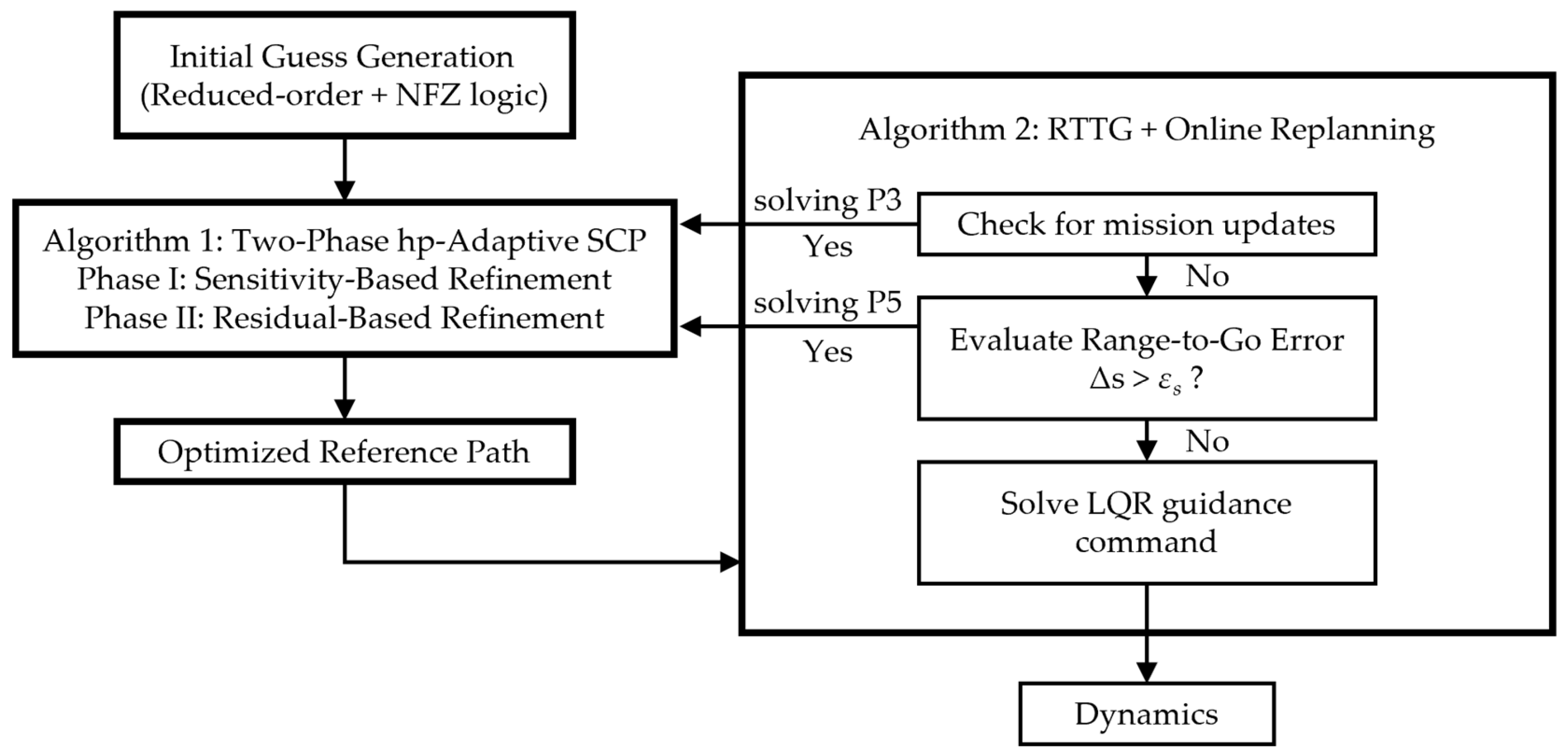
4.3. Reference-Trajectory-Tracking Guidance (RTTG) Algorithm

4.3.1. Initial Guess Generation

Iterative algorithms for constrained or unconstrained optimization typically require an initial guess. While such a guess may be arbitrarily selected, a more effective approach leverages problem-specific insights to construct a solution estimate that is both feasible and close to optimal.

To generate a fully constrained initial guess for the proposed two-stage trajectory optimization framework, we adopt a combined initialization strategy based on our previously developed reduced-order entry guidance method [39] and the dynamic heading corridor technique [40].

Specifically, a tailored altitude–velocity (H-V) profile is first constructed in the longitudinal channel to satisfy the desired terminal time constraint. This is achieved by parameterizing the H-V curve with a shaping parameter k_H, which controls the altitude level of the glide segment. The time-to-go (TTG) along this profile is computed via integration of the reduced-order longitudinal dynamics. A Newton-based predictor–corrector iteration is then used to determine the optimal value of k_H that matches the desired TTG, resulting in a dynamically feasible reference profile that satisfies aerodynamic path constraints as well as terminal altitude and velocity requirements.

In the lateral channel, the heading offset is adjusted through a bank-reversal logic, in which the sign of the bank angle is reversed whenever the heading offset exceeds a predefined, velocity-dependent threshold. This mechanism enables range-to-go (RTG) adjustment while tracking the longitudinal reference, ensuring compliance with both terminal range and heading constraints. Three-dimensional reduced-order dynamics are integrated to predict the trajectory outcome and to iteratively refine the heading threshold.

To further accommodate complex NFZ constraints, the dynamic heading corridor strategy proposed in [40] is incorporated into the lateral planning process. This method constructs a chain-mode heading corridor by recursively intersecting the terminal line-of-sight (LOS) corridor with tangent-derived exclusion angles of each NFZ, processed in order from farthest to nearest. The resulting time-varying corridor imposes adaptive heading constraints, and the bank-reversal logic is extended accordingly to ensure that the trajectory remains within this dynamically shrinking safe envelope. This combined strategy yields an initial trajectory that satisfies all path constraints, terminal conditions, and NFZ avoidance requirements, providing a high-quality starting point for the subsequent SCP refinement process.

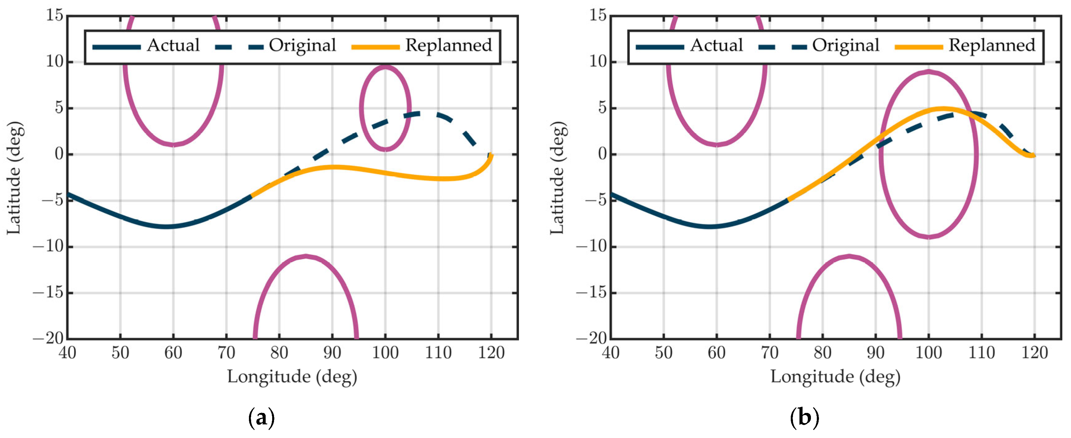
4.3.2. Trajectory Tracking and Online Correction

Building upon the initial guess described in Section 4.3.1, Algorithm 1 is employed to generate the nominal reference trajectory at the atmospheric entry interface by solving Problem P3.

This reference trajectory is subsequently tracked using a linear quadratic regulator (LQR), with the control input defined as follows:

$$u_{\mathrm{cmd}}=u_{\mathrm{ref}}-K\mathsf{\Delta }X,$$

(73)

where u_ref = [α_ref, σ_ref] is the reference control command, K is the precomputed feedback gain matrix, and ∆X = [∆r, ∆V, ∆γ]^T denotes the longitudinal tracking error in altitude, velocity, and flight-path angle.

To enhance robustness against parametric uncertainties, a correction filter—adapted from [41]—is applied to the computed aerodynamic accelerations in Equation (45). This filter adjusts lift and drag values based on real-time feedback to mitigate modeling errors. Additionally, all path constraints are conservatively tightened using a safety factor C_s < 1, ensuring feasibility under bounded disturbances.

The RTTG architecture also supports real-time trajectory correction through an online replanning mechanism. At each guidance cycle, the RTG deviation Δs—defined as the great-circle distance between the current vehicle location and the nominal reference—is evaluated. If Δs exceeds a user-defined threshold ε_s, the reference trajectory is regenerated to compensate for accumulated deviations or external perturbations.

The complete guidance logic is summarized in Algorithm 2:

Algorithm 2. RTTG with Online Reference Trajectory Updates
Step	Procedure
1	Initialize vehicle states, constraints, and all relevant parameters. Generate an initial reference guess.
2	Compute the reference trajectory via Algorithm 1 (solving Problem P3).
3	If t ≥ tf, terminate guidance; otherwise, proceed to Step 4.
4	Check for mission updates (e.g., NFZ changes). If applicable, return to Step 2; otherwise, continue.
5	Evaluate the RTG deviation ∆s. If ∆s > εs, recompute the trajectory by solving Problem P5.
6	Apply the LQR guidance command via Equation (73), and return to Step 3.

To improve readability and provide a clear overview of the proposed framework, a high-level flowchart summarizing the methodology is presented in Figure 2. It captures the entire process from initial guess generation and two-phase trajectory optimization to closed-loop trajectory tracking and online replanning. This visualization complements Algorithms 1 and 2 by clarifying their interaction within the overall architecture.

5. Results and Analysis

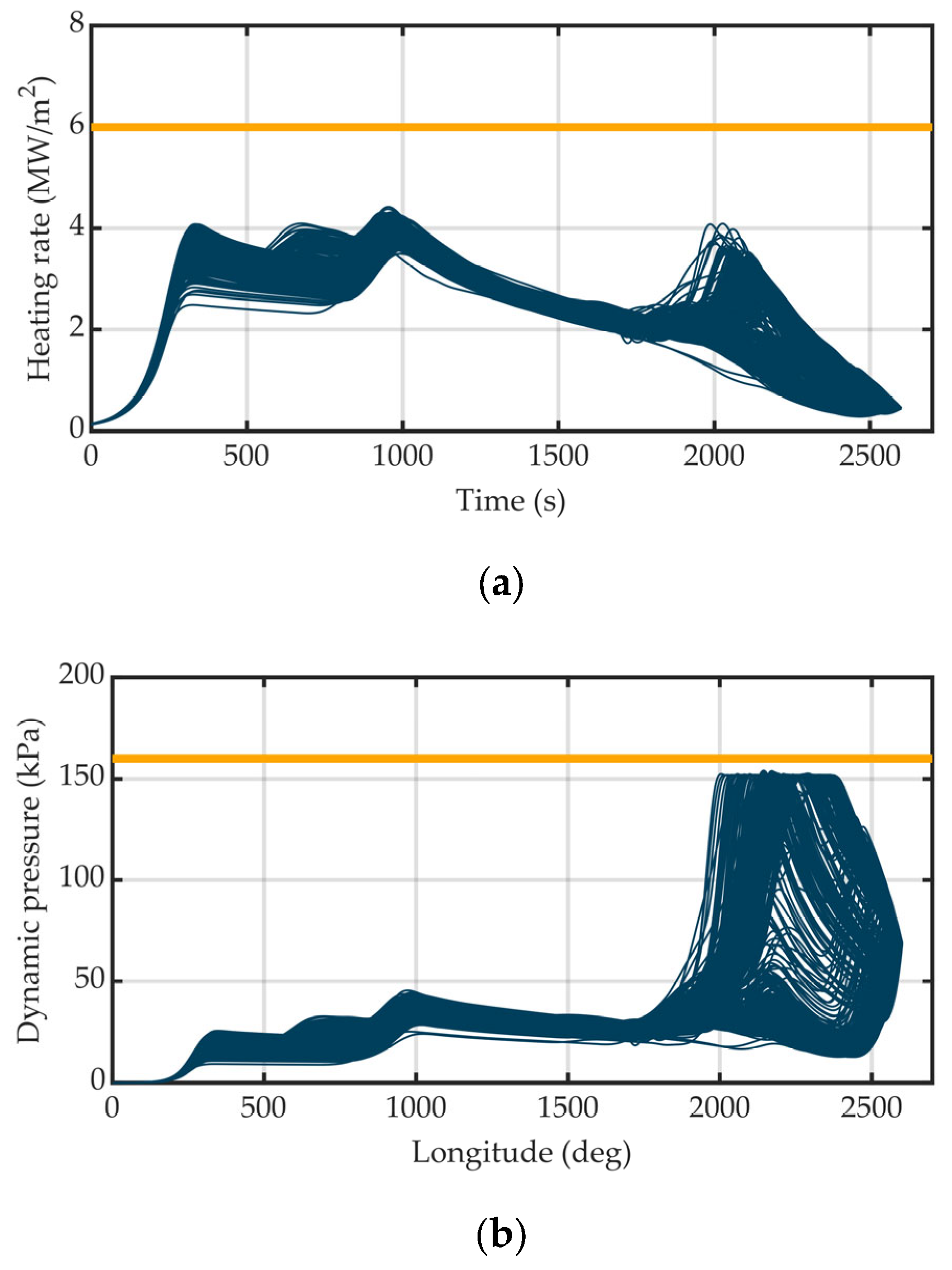
5.1. Simulation Conditions

To validate the proposed guidance algorithm, numerical simulations were conducted using the CAV-H vehicle model [42]. The terminal flight time was set to t_f = 2600 s. The initial conditions, target terminal state, and state bounds are summarized in

Table 1. Boundary conditions and bounds of the states.

State	H (km)	θ (deg)	ϕ (deg)	V (m/s)	γ (deg)	ψ (deg)	α (deg)	σ (deg)
x0	120	0	0	7200	−1	90	\ 1	\
xf	25	120	0	2000	\	\	\	\
xmin	25	−180	−90	2000	-5	0	5	−80
xmax	120	180	90	7500	0	360	25	80

¹ “\” indicates that no constraints have been imposed.

. Control inputs were constrained to reflect realistic actuator limitations as follows:

$$\left|\dot{\alpha }\right|\le 5 \mathrm{deg}/\mathrm{s},\hspace{0.33em}\left|\dot{\sigma }\right|\le 10 \mathrm{deg}/\mathrm{s}.$$

Path constraints included a maximum heating rate of Q_max = 6 MW/m², a maximum dynamic pressure of q_max = 160 kPa, and a maximum load factor of n_max = 3 g. In the objective function, the optimization weight coefficients were set as follows:

$$C_1=2\times {10}^{-3},\hspace{0.33em}{C}_2=5\times {10}^{-4},\hspace{0.33em}{C}_3=1\times {10}^{-4}.$$

Mesh refinement was governed by the following parameters:

$$\begin{array}{c}{N}_{\min }=4,\hspace{0.33em}{N}_{\max }=16,\hspace{0.33em}{N}_{\mathrm{add} }=8,\hspace{0.33em}{\beta }_{\max }=2,\hspace{0.33em}{C}_{\mathrm{div} }=1.2,\\ {\epsilon }_{p1}=1.5,\hspace{0.33em}{\epsilon }_{p2}=1.1,\hspace{0.33em}{\epsilon }_{\delta }=5\times {10}^{-3},\hspace{0.33em}{\epsilon }_e=1\times {10}^{-3}.\end{array}$$

A safety factor of C_s = 0.95 was applied to all path constraints to account for modeling and execution uncertainties. The initial mesh consisted of Y⁽⁰⁾ = 10 uniform intervals, each initialized with N⁽⁰⁾ = 5 LGR collocation points. A tracking deviation threshold of ε_s = 10 km was imposed to trigger trajectory replanning. Two NFZ constraints were included, with their geometric parameters provided in

Table 2. Center and radius of NFZs.

NFZ No.	Center (θ, ϕ) (deg)	Radius (km)
NFZ 1	(60, 10)	1000
NFZ 2	(85, −20)	1000

.

Each SOCP subproblem was formulated using the CVX modeling framework [43] and solved using the MOSEK solver [44]. All simulations were carried out in MATLAB R2021b on a desktop computer equipped with an AMD Ryzen 7 5800X processor (Advanced Micro Devices, Inc., Santa Clara, CA, USA).

5.2. Influence of the Soft-Trust-Region Weight

Before implementing the two-phase hp-adaptive strategy proposed in Algorithm 1, we first examine how a fixed soft-trust-region weight C₃ affects the convergence behavior of SCP on a static mesh. These results offer practical guidance for selecting the initial value C₃, the upper bound C_3,max, and the growth factor k₃ used in Phase I.

The simulation uses a fixed mesh of 10 intervals, each containing 20 LGR collocation points, totaling 201 discretization nodes. In each test, the trust-region formulation is kept soft and the weight C₃ is fixed throughout the run. Six penalty values are evaluated: C₃ ∈ {10⁻⁵, 10⁻⁴, 10⁻³, 10⁻², 10⁻¹, 1}. The convergence criterion is consistent with the Phase II residual tolerance (e_max < ε_e), and each run is capped at 30 iterations.

Figure 3 illustrates the evolution of re-integrated ground tracks (longitude versus latitude) over iterations for each penalty weight. Figure 4 further summarizes two key performance indicators: the Euclidean norm of the soft trust-region radius ${‖{\delta }_{\mathrm{soft}}‖}_2$ and the maximum relative discretization error e_max.

The results show that for low penalty values (10⁻⁵ to 10⁻³), the trust region remains large, enabling wide exploration of the decision space. However, the persistent large radius leads to significant linearization error, preventing convergence within 30 iterations. In particular, since the NFZ-avoidance term depends on the linearized constraint formulation, excessive linearization error undermines its reliability in the objective function. In contrast, moderate penalties (10⁻² and 10⁻¹) induce gradual contraction of the trust region and reduction in linearization error, resulting in convergence after 13 and 3 iterations, respectively. When the penalty weight is too large (C₃ = 1), the trust region shrinks too aggressively—often collapsing below 10⁻⁵—which overly restricts the feasible space and traps the solver in a poor local minimum. In this case, the residual stagnates and fails to reach the desired tolerance.

Based on these observations, we configure Phase I with an initial penalty C₃ = 10⁻⁴, an upper bound C_3,max = 10⁻¹, and a multiplicative growth factor k₃ = 10. This setting allows the trust region to start permissive for global exploration and then shrink progressively as iterations proceed until the average radius satisfies the condition in Equation (56).

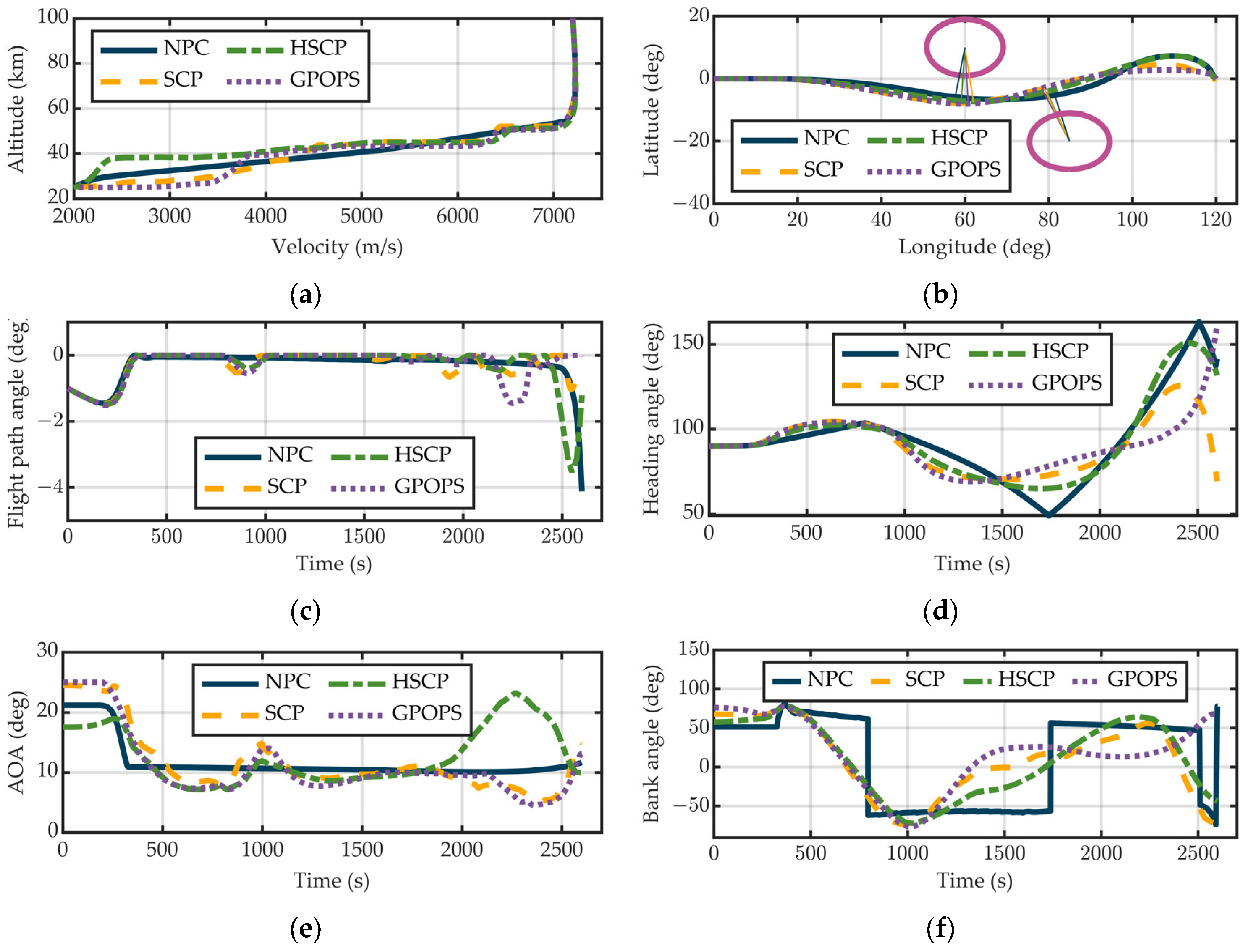
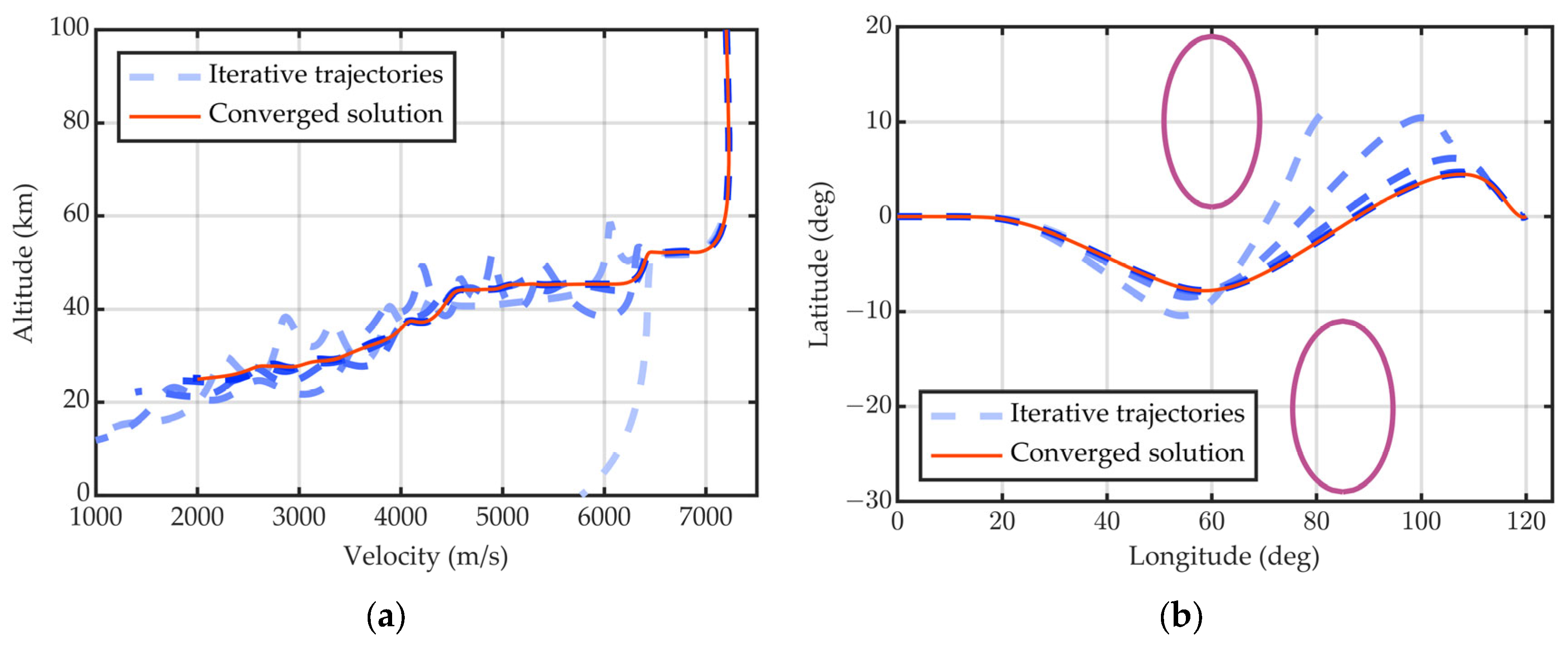
5.3. Nominal-Case Reference Trajectory

With the soft-trust-region weights fixed to the values determined in Section 5.2, Algorithm 1 is executed under nominal atmospheric and vehicle parameters to generate a baseline reference trajectory.

• Two variants are considered:

• SCP—the default first-order soft-trust-region formulation (Problem P3).
• HSCP—a fourth-order soft-trust-region formulation obtained by replacing P3 with P4 and setting C₃ = 10⁻³ and C_3,max = 100.

• For comparison, we also include the following:

• NPC—the numerically predicted-corrected guess described in Section 4.3.1.
• GPOPS—the global optimum computed off-line with GPOPS-II [38].

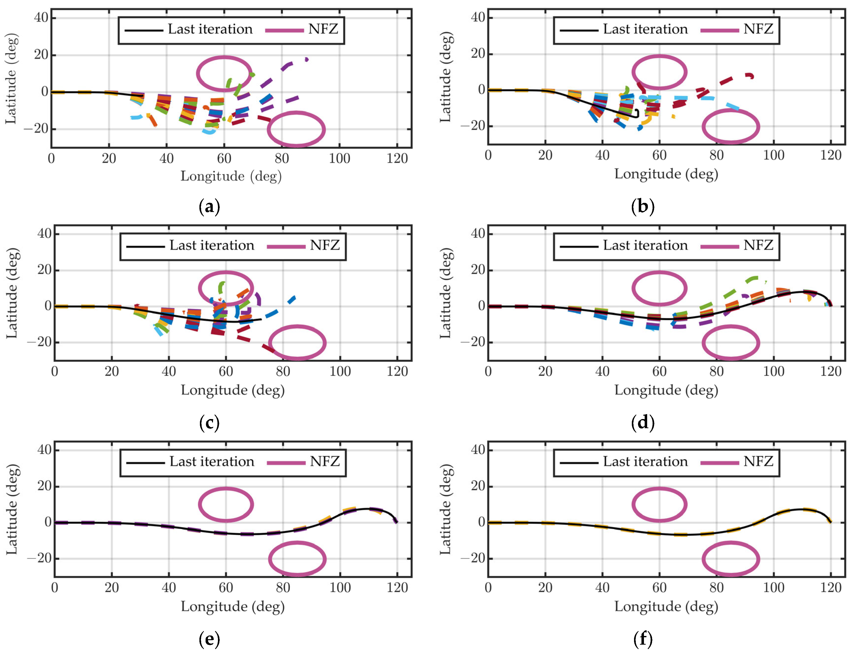
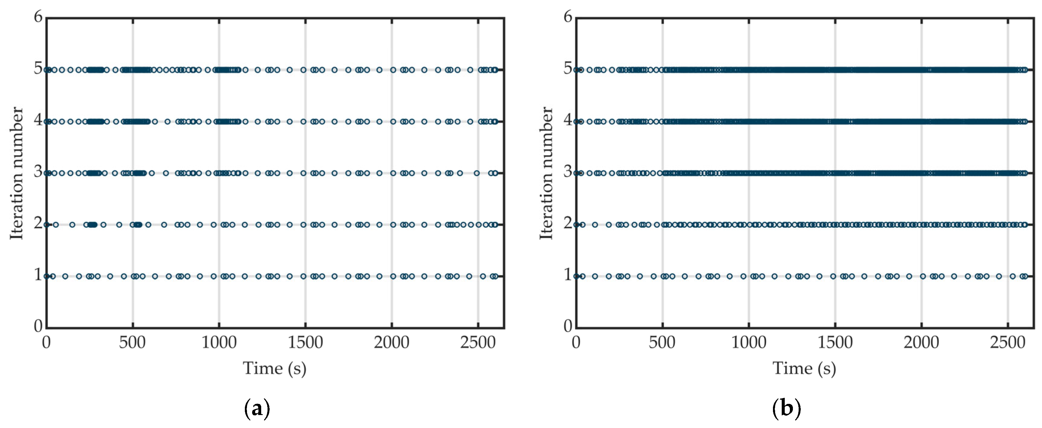
• Comparative results are illustrated in Figure 5.

From the ground-track plot (Figure 5b), the minimum clearance margin to the two NFZs is listed in

Table 3. Minimum clearance margin to NFZs.

Trajectory	NPC	SCP	HSCP	GPOPS
NFZ 1 (km)	780.0	974.4	909.7	1015.2
NFZ 2 (km)	682.6	990.4	867.6	1015.2

. The GPOPS solution, as expected, balances the two separations perfectly. Relative to the NPC baseline, the SCP trajectory enlarges the safety margins by 24.92% (NFZ 1) and 45.09% (NFZ 2); HSCP falls in between.

Figure 5. Reference-trajectory comparison: (a) altitude vs. velocity, (b) ground track (longitude-latitude), (c) flight-path angle vs. time, (d) heading angle vs. time, (e) AOA vs. time, and (f) bank angle vs. time.

Figure 5. Reference-trajectory comparison: (a) altitude vs. velocity, (b) ground track (longitude-latitude), (c) flight-path angle vs. time, (d) heading angle vs. time, (e) AOA vs. time, and (f) bank angle vs. time.

Figure 6 depicts the convergence index evolution during the iterative solving process. Phase I meets the trust-region tolerance after 5 iterations, whereupon Phase II is activated. Convergence is declared 2 iterations later when the maximum relative defect drops to 9.54 × 10⁻⁴. The entire SCP optimization thus terminates in 7 iterations/2.01 s, whereas the off-line GPOPS computation requires 10 iterations/24.75 s, i.e., a 12.3× speed-up.

Although the resulting trajectory is slightly suboptimal compared with the global solution, the dramatic reduction in CPU time fulfills the primary design goal of enabling on-board real-time planning. HSCP, despite using a higher-order trust region, does not improve NFZ clearance in this case and incurs a larger computational cost (2.33 s) because of the extra auxiliary variables and constraints. When both SCP and HSCP already meet mission requirements, the lower-order variant is therefore preferred. In summary, the proposed hp-adaptive SCP framework trades a modest amount of optimality for speed, robustness, and implementability—qualities that are paramount for practical entry-guidance systems.

Figure 7 compares the evolution of the pseudospectral grid during Phase I refinement using two methods:

• sensitivity-based refinement (proposed),
• residual-based refinement (baseline).

Both schemes satisfy the Phase-I trust-region tolerance in five iterations, yet their computational footprints differ markedly.

• Sensitivity strategy: average 100 nodes·per iteration, total CPU time = 1.23 s.
• Residual strategy: average 334 nodes·per iteration, total CPU time = 3.86 s.

Focusing refinement on states with the highest adjoint-based sensitivity packs grid points where they matter most, delivering a much leaner and nearly 3× faster optimization without degrading convergence accuracy.

Solver-level feasibility was attained at every iteration, yet the open-loop truth-model integrations of the optimized controls initially diverged noticeably from their pseudospectral references. Figure 8 tracks this discrepancy over the successive meshes as follows:

• Iterations 1–3—the coarse 50-node grid under-resolves the dynamics; integrated ground-track errors exceed 1000 km.
• Progressive refinement—as hp-adaptation concentrates points in sensitive segments, the mismatch contracts rapidly.
• Final mesh—with 181 nodes, the maximum deviations shrink to altitude = 277 m, velocity = 5.5 m/s, and RTG = 3.8 km.

Overall, the open-loop error drops three orders of magnitude, falling well below the 10 km repositioning threshold required by the real-time trajectory-tracking guidance (Algorithm 2). This outcome confirms that the combined trust-region and hp-adaptive strategy enforces both constraint satisfaction and true-trajectory fidelity.

To test real-time obstacle handling, two notional NFZs were announced on-the-fly when the vehicle was still 3000 km away: Scenario 1—NFZ centered at (100°, 5°) with a 500 km radius, and Scenario 2—NFZ centered at (100°, 0°) with a 1000 km radius. At detection, Algorithm 2 paused tracking, solved a fresh guidance problem, and then resumed closed-loop execution.

• Scenario 1—modest obstacle (Figure 9a)

The regenerated path threads cleanly between all restricted areas; the closest approach to any boundary is 316 km. Re-optimization required 2.82 s.

• Scenario 2—large obstacle (Figure 9b)

Because the 1000 km NFZ spans nearly the entire lateral envelope, complete avoidance is impossible without gross mission deviation. The planner therefore minimizes risk by skirting the critical core while accepting a shallow incursion into its low-hazard periphery: the trajectory passes 522 km from the center (i.e., 478 km inside the outer limit). The computation finished in 2.87 s.

These results demonstrate that the hp-adaptive SCP framework replans quickly enough for onboard use, balancing feasibility, safety margins, and vehicle maneuverability even under stringent, late-notice NFZ constraints.

5.4. Computational Performance and Complexity

This section analyzes the computational performance of the proposed two-phase hp-adaptive SCP framework and compares it against a high-fidelity pseudospectral solver to assess its suitability for real-time, onboard implementation.

The proposed SCP method completes trajectory optimization in seven iterations—five in Phase I and two in Phase II—with a total runtime of 2.01 s on a standard desktop platform. The number of discretization nodes increases adaptively from 50 to 165 during Phase I, followed by a refinement to 180 nodes in Phase II. Each iteration takes less than 0.4 s, with the fastest at 0.06 s and the slowest at 0.40 s. This efficiency is largely attributed to the sensitivity-driven mesh refinement strategy, which focuses resolution on dynamically sensitive segments without excessively increasing the problem size.

In contrast, GPOPS-II employs an hp-adaptive Radau pseudospectral discretization and solves the resulting NLPs using SNOPT. Across 10 mesh refinement iterations, the number of collocation points grows from 40 to 461, and the number of optimization variables increases from 412 to 4622. The overall solution requires 24.75 s, making SCP over 12 times faster under equivalent benchmark settings.

To further quantify solver complexity, we examine floating-point operation counts (FLOPs) using solver-level diagnostics. For a typical SCP subproblem with 9217 decision variables and 2524 equality constraints, the MOSEK solver performs 38 interior-point iterations. Each iteration involves approximately 2.67 × 10⁶ FLOPs, resulting in a total of 1.0 × 10⁸ FLOPs for the complete SCP process.

In comparison, GPOPS-II’s use of dense Jacobians and global collocation structures leads to significantly higher computational demands. Its final NLP includes over 4600 variables and 5996 constraints, and the underlying SQP method executes over 1100 minor iterations. Even conservatively estimated, the total FLOPs exceed 4 × 10⁹, making GPOPS approximately 40 to 60 times more computationally intensive than the proposed SCP approach.

These results validate the computational efficiency of the proposed method. Its ability to maintain low solver complexity, fast convergence, and accurate mesh adaptivity underpins its practical usability for onboard, real-time trajectory optimization in hypersonic entry scenarios.

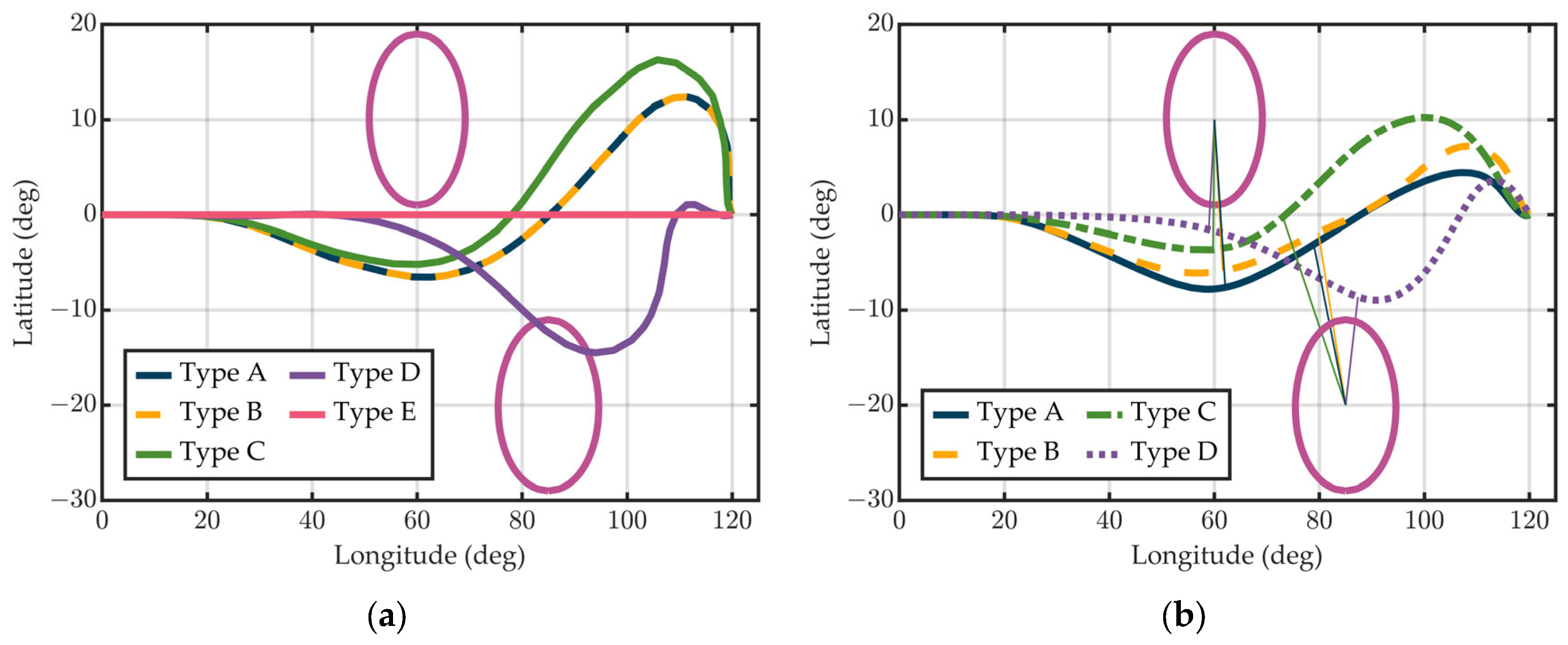
5.5. Sensitivity Study on Initial Guess Quality

To evaluate the robustness of the proposed two-phase hp-adaptive SCP framework with respect to the quality of the initial trajectory guess, a series of sensitivity experiments were conducted under a fixed entry scenario. Five different initialization strategies were tested, as summarized below:

(A)

Proposed Method: The combined approach using the reduced-order guidance method [39] and the dynamic heading corridor strategy [40], which satisfies all constraints.

(B)

Perturbed Trajectory (H + ψ): Gaussian noise added to the initial altitude and heading profile of the proposed method.

(C)

Perturbed Trajectory (All States): Random perturbations applied to all state variables along the trajectory.

(D)

Degraded Trajectory: Initialization using [39] only, without considering NFZ constraints.

(E)

Straight-Line Trajectory: A naively constructed trajectory by linearly interpolating all state variables from the initial point to the terminal point.

All five trajectories were used as starting points for the two-phase SCP process. The results are summarized in

Table 4. Sensitivity analysis of initial guess quality on SCP performance.

Initial Guess Type	Converged?	Total Iterations	Time (s)	Minimum Distance to NFZ 1 (km)	Minimum Distance to NFZ 2 (km)
(A) Proposed Method	Yes	7	2.01	974.4	990.4
(B) Perturbed H + ψ	Yes	8	2.04	774.6	1096.2
(C) Perturbed All States	Yes	8	3.16	520.2	1552.7
(D) Degraded (No NFZ)	Yes	10	3.91	289.6	291.1
(E) Straight-Line	No	–	–	–	–

, reporting convergence status, total iteration count, total computation time, and the minimum distance to the two NFZs.

As expected, lower-quality initial guesses generally result in longer optimization times and reduced NFZ clearance. Nevertheless, for all converged cases (A–D), the optimized control profiles yield open-loop truth-model trajectories with excellent fidelity.

Figure 8 previously demonstrated how the hp-adaptive strategy progressively refines the mesh to resolve true dynamics, shrinking the integration errors to below operational thresholds. This trend holds across different initial guesses: although convergence effort varies, the final integrated trajectories consistently match their corresponding optimized references with high accuracy.

To quantify the final trajectory accuracy under different initialization strategies,

Table 5. Maximum integration errors under different initial guesses.

Initial Guess Type	Max Altitude Error (m)	Max Velocity Error (m/s)	Max RTG Error (km)
(A) Proposed Method	277	5.5	3.8
(B) Perturbed H + ψ	114	3.4	1.6
(C) Perturbed All States	292	11.5	4.5
(D) Degraded (No NFZ)	379	19.2	5.8

reports the maximum deviations between the open-loop integrated trajectory and its optimized reference at the final mesh. As shown, for all converged cases (A–D), the integration errors in altitude, velocity, and RTG remain small and within acceptable bounds for real-time execution. This further confirms that the hp-adaptive refinement effectively controls discretization error regardless of the initial guess quality.

To further visualize the effect of different initial guesses, Figure 10 presents the ground-track projections of all five initialization strategies, along with the resulting optimized trajectories for the converged cases (A–D). While the initial guesses vary significantly—particularly in the degraded and straight-line cases—the converged solutions successfully redirect the vehicle toward the target while ensuring avoidance of all NFZs. Although the optimized trajectories differ in shape and constraint clearance margins, they all satisfy the terminal conditions and demonstrate successful guidance to the target region. The straight-line initialization (Case E) failed to converge, and therefore no optimized trajectory is shown for that case.

These results confirm that the proposed initialization method (Case A) enables fast convergence and superior constraint satisfaction. Moreover, trajectory fidelity is consistently maintained across all converged cases, regardless of the initial guess quality.

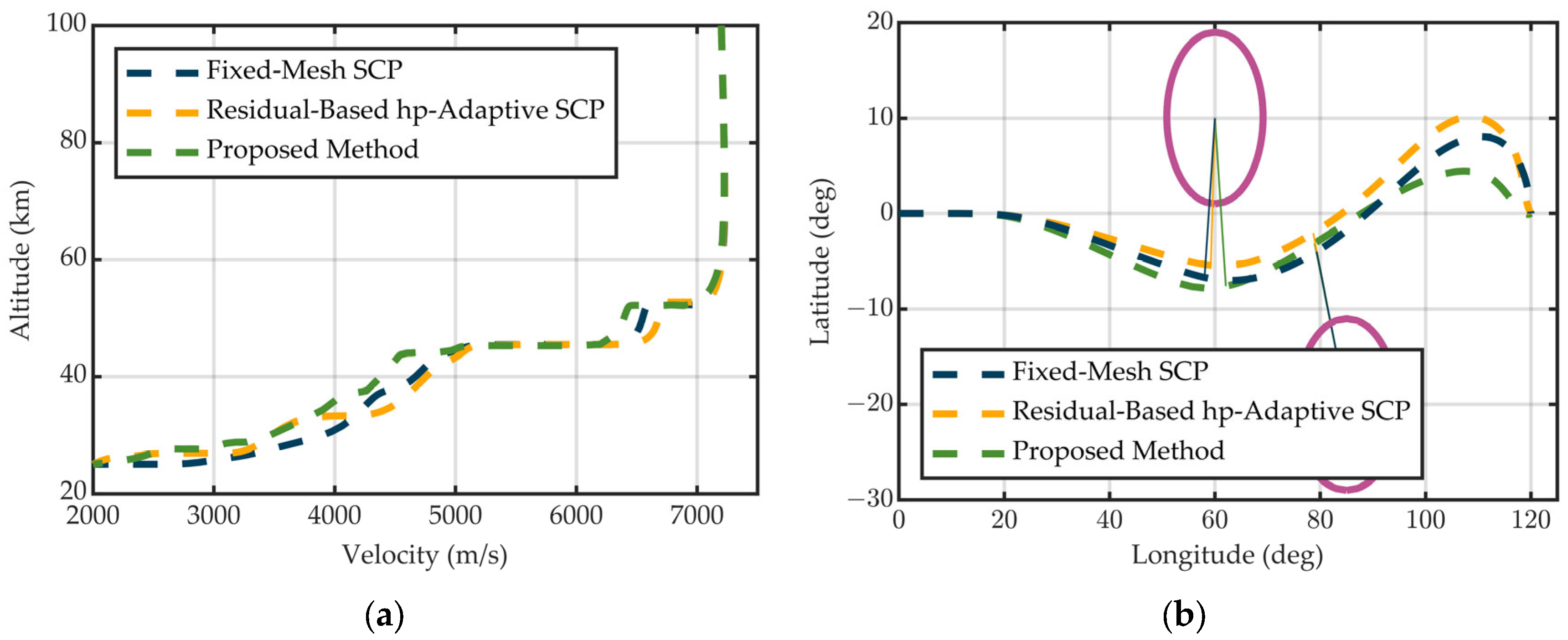
5.6. Comparison with Alternative SCP-Based Methods

To highlight the performance advantages of the proposed two-phase hp-adaptive SCP framework, we conduct a comparative study involving two alternative SCP variants commonly found in the literature:

• Fixed-Mesh SCP: A single-stage SCP algorithm employing a fixed pseudospectral mesh of 10 segments with 20 LGR points per segment (201 total nodes). The soft-trust-region weight is held constant at C₃ = 10⁻², corresponding to the moderate-penalty configuration from Section 5.2.
• Residual-Based hp-Adaptive SCP: An hp-refined variant using residual-driven mesh adaptation at all iterations. This method applies the same initial mesh and refinement logic as Phase II of our proposed method, but without separating the linearization and discretization error handling.
• Proposed Method: The two-phase strategy introduced in this paper, using sensitivity-guided refinement in Phase I and residual-driven refinement in Phase II, with dynamic trust-region weights to balance global exploration and local convergence.

All three methods are evaluated under identical initial and terminal conditions, with consistent convergence criteria based on the maximum relative discretization error. Their resulting trajectories are shown in Figure 11, including altitude–velocity profiles and ground-track projections.

In terms of computational performance, the three methods exhibit markedly different behavior. The fixed-mesh SCP converges in 13 iterations and requires 7.78 s. Due to the lack of adaptive mesh refinement, it struggles to resolve localized dynamics and requires dense meshing from the outset. The residual-based hp-adaptive method converges in 6 iterations but incurs 4.78 s of runtime, with an average of 383 nodes per iteration—significantly more than the proposed method. This is because residual-driven refinement, when applied during early iterations where linearization errors dominate, tends to over-refine the mesh in low-priority regions.

In contrast, the proposed method achieves convergence in just 7 iterations and 2.01 s, with an average of 121 nodes per iteration. This outcome validates the efficiency of the two-phase refinement strategy: sensitivity-based refinement in Phase I concentrates nodes where they most affect trajectory shaping, while residual-based refinement in Phase II polishes the solution only after linearization errors are sufficiently reduced.

The minimum clearance margin to the NFZs for the fixed-mesh and residual-based methods are 871.7 km and 718.0 km, respectively, compared to 974.4 km achieved by the proposed approach. This superior clearance indicates that the dynamic trust-region scaling in Phase I improves the reliability of the linearized NFZ-avoidance objective, enabling safer and more robust trajectories.

In summary, this comparative study demonstrates that the proposed method achieves a favorable trade-off among convergence speed, computational cost, mesh efficiency, and constraint robustness—attributes critical for real-time onboard guidance systems. The combination of adaptive refinement and dynamic trust-region control distinguishes the method from both static and single-phase alternatives.

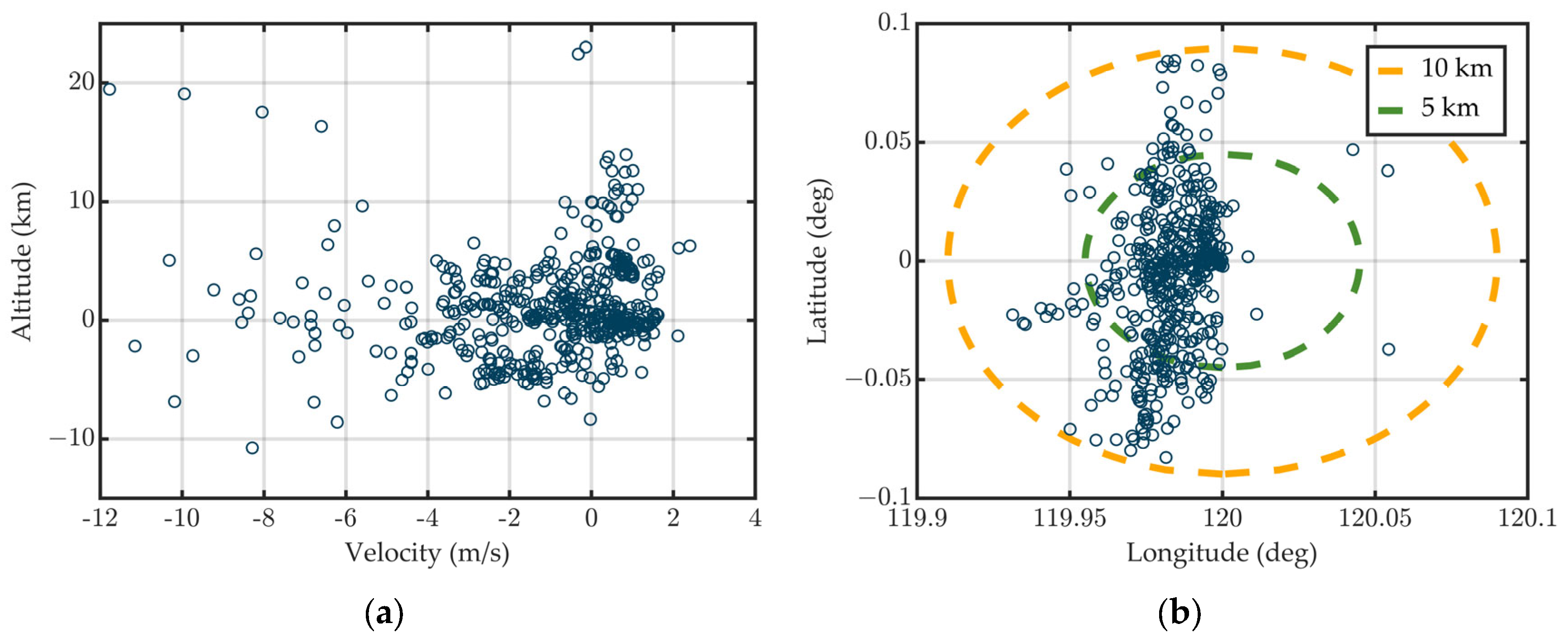
5.7. Monte Carlo Assessment with Dispersed Parameters

To probe the algorithm’s robustness, we injected simultaneous, zero-mean Gaussian perturbations (3-sigma limits listed in

Table 6. Dispersion settings.

Parameter	H0 (km)	θ0 (deg)	φ0 (deg)	V0 (m/s)	γ0 (deg)	ψ0 (deg)	m	ρ	CL	CD
3-sigma	1	0.5	0.5	20	0.1	0.5	5%	10%	10%	10%

) into the initial state, atmospheric density (multiplicative bias), vehicle mass, and lift/drag coefficients. A 500-shot Monte Carlo campaign was run. The simulation results are shown in Figure 12. Algorithm 1 generated feasible reference trajectories in all 500 runs; no convex-solver or convergence failures occurred.

Figure 13 pools the statistical outcomes. The dispersions at the terminal interface are tightly bounded as follows:

• Altitude ±25 m (≈0.1% of nominal).
• Velocity ±12 m/s (≈0.6% of nominal).
• Down-range ±10 km (≈0.07% of total range).

All samples remain well inside the mission tolerances.

Figure 14 overlays the 500 trajectories against the heating rate, dynamic pressure, and load factor envelopes. Every realization respects the limits, confirming that the tightened constraints and online re-planning logic furnish statistical guarantees of safety.

Across a realistically dispersed flight envelope, the hp-adaptive SCP/RTTG framework delivers 100% mission success: it maintains constraint satisfaction, meets terminal-state requirements, and shows no numerical fragility. These results underscore the method’s suitability for operational guidance in uncertain atmospheric-entry scenarios.

6. Conclusions

This paper proposed a two-phase hp-adaptive SCP framework for real-time trajectory generation in HGV entry guidance under multiple competing constraints, including aerothermal loads, dynamic pressure, control limits, and NFZs. By reformulating NFZ avoidance as a soft objective, the method enables feasible trajectory planning even under infeasible obstacle conditions, improving robustness compared to traditional hard-constrained approaches.

To address both linearization and discretization errors in SCP, a staged strategy was developed: Phase I employs a shrinking soft-trust-region mechanism with sensitivity-driven mesh refinement, ensuring rapid and stable convergence; Phase II uses residual-driven refinement to achieve high-accuracy trajectory solutions. The generated reference trajectory is then tracked by a LQR within a RTTG architecture.

Simulation results under nominal and dynamic scenarios demonstrate the method’s efficiency and robustness: feasible solutions are consistently obtained in less than 3 s, and trajectory quality approaches pseudospectral benchmarks with a ~12× computational speed-up. In a 500-sample Monte Carlo test under uncertainties, the framework achieved 100% mission success without violating constraints or incurring solver failures.

Nonetheless, the proposed method sacrifices a degree of trajectory optimality due to the use of linearized convex surrogates in each iteration. While this trade-off is acceptable for time-critical onboard applications, future research will focus on reducing this optimality gap—potentially via hybrid schemes that integrate global nonlinear programming stages or higher-order convex relaxations—thereby enhancing performance without compromising real-time feasibility.

Overall, the proposed SCP-based guidance framework offers a reliable, fast, and scalable trajectory-planning solution well-suited for constrained entry missions in realistic operational environments.

References

1. Lu, P. Entry guidance: A unified method. J. Guid. Contr. Dyn. 2014, 37, 713–728. [Google Scholar] [CrossRef]
2. Yu, W.; Yang, J.; Chen, W. Entry guidance based on analytical trajectory solutions. IEEE Trans. Aerosp. Electron. Syst. 2021, 58, 2438–2466. [Google Scholar] [CrossRef]
3. Guo, Y.; Li, X.; Zhang, H.; Wang, L.; Cai, M. Entry guidance with terminal time control based on quasi-equilibrium glide condition. IEEE Trans. Aerosp. Electron. Syst. 2019, 56, 887–896. [Google Scholar] [CrossRef]
4. Liu, Z.; Zheng, G.; Zhang, B.; Wei, J.; Huang, H.; Yan, J. Predictor-corrector reentry guidance for hypersonic glide vehicles based on high-precision analytical solutions. Aerosp. Sci. Technol. 2024, 155, 109545. [Google Scholar] [CrossRef]
5. Liang, Z.; Lv, C.; Zhu, S. Lateral entry guidance with terminal time constraint. IEEE Trans. Aerosp. Electron. Syst. 2022, 59, 2544–2553. [Google Scholar] [CrossRef]
6. Wang, H.; Guo, J.; Wang, X.; Li, X.; Tang, S. Time-coordination entry guidance using a range-determined strategy. Aerosp. Sci. Technol. 2022, 129, 107842. [Google Scholar] [CrossRef]
7. Yao, D.; Xia, Q. Predictor-corrector guidance for a hypersonic morphing vehicle. Aerospace 2023, 10, 795. [Google Scholar] [CrossRef]
8. Dukeman, G. Profile-following entry guidance using linear quadratic regulator theory. In Proceedings of the AIAA Guidance, Navigation, and Control Conference and Exhibit, Monterey, CA, USA, 5–8 August 2002. [Google Scholar] [CrossRef]
9. Mease, K.D.; Chen, D.T.; Teufel, P.; Schönenberger, H. Reduced-order entry trajectory planning for acceleration guidance. J. Guid. Contr. Dyn. 2002, 25, 257–266. [Google Scholar] [CrossRef]
10. Guo, J.; Wu, X.; Tang, S. Autonomous gliding entry guidance with geographic constraints. Chin. J. Aeronaut. 2015, 28, 1343–1354. [Google Scholar] [CrossRef]
11. Wang, X.; Guo, J.; Tang, S.; Qi, S.; Wang, Z. Entry trajectory planning with terminal full states constraints and multiple geographic constraints. Aerosp. Sci. Technol. 2019, 84, 620–631. [Google Scholar] [CrossRef]
12. Zhang, Y.; Xie, Y.; Peng, S.; Tang, G.; Bao, W. Entry trajectory generation with complex constraints based on three-dimensional acceleration profile. Aerosp. Sci. Technol. 2019, 91, 231–240. [Google Scholar] [CrossRef]
13. Wang, Z.; Grant, M.J. Autonomous entry guidance for hypersonic vehicles by convex optimization. J. Spacecr. Rockets 2018, 55, 993–1006. [Google Scholar] [CrossRef]
14. Wu, Y.; Yao, J.; Qu, X. An adaptive reentry guidance method considering the influence of blackout zone. Acta Astronaut. 2018, 142, 253–264. [Google Scholar] [CrossRef]
15. Sana, K.S.; Hu, W. Hypersonic reentry trajectory planning by using hybrid fractional-order particle swarm optimization and gravitational search algorithm. Chin. J. Aeronaut. 2021, 34, 50–67. [Google Scholar] [CrossRef]
16. Kabganian, M.; Hashemi, S.M.; Roshanian, J. Multidisciplinary design optimization of a re-entry spacecraft via Radau pseudospectral method. Appl. Mechanics 2022, 3, 1176–1189. [Google Scholar] [CrossRef]
17. Ma, S.; Yang, Y.; Yang, H.; Chen, W. Trajectory optimization of hypersonic vehicle considering the quasi-static assumption of pitch motion. Aerosp. Sci. Technol. 2024, 146, 108969. [Google Scholar] [CrossRef]
18. Mu, L.; Cao, S.; Wang, B.; Zhang, Y.; Feng, N.; Li, X. Pseudospectral-based rapid trajectory planning and feedforward linearization guidance. Drones 2024, 8, 371. [Google Scholar] [CrossRef]
19. Acikmese, B.; Ploen, S.R. Convex programming approach to powered descent guidance for Mars landing. J. Guid. Contr. Dyn. 2007, 30, 1353–1366. [Google Scholar] [CrossRef]
20. Açıkmeşe, B.; Blackmore, L. Lossless convexification of a class of optimal control problems with non-convex control constraints. Automatica 2011, 47, 341–347. [Google Scholar] [CrossRef]
21. Liu, X.; Shen, Z. Rapid smooth entry trajectory planning for high lift/drag hypersonic glide vehicles. J. Optim. Theory Appl. 2016, 168, 917–943. [Google Scholar] [CrossRef]
22. Liu, X.; Shen, Z.; Lu, P. Solving the maximum-crossrange problem via successive second-order cone programming with a line search. Aerosp. Sci. Technol. 2015, 47, 10–20. [Google Scholar] [CrossRef]
23. Liu, X.; Shen, Z.; Lu, P. Entry trajectory optimization by second-order cone programming. J. Guid. Contr. Dyn. 2016, 39, 227–241. [Google Scholar] [CrossRef]
24. Wang, Z.; Grant, M.J. Constrained trajectory optimization for planetary entry via sequential convex programming. J. Guid. Contr. Dyn. 2017, 40, 2603–2615. [Google Scholar] [CrossRef]
25. Zhao, D.; Song, Z. Reentry trajectory optimization with waypoint and no-fly zone constraints using multiphase convex programming. Acta Astronaut. 2017, 137, 60–69. [Google Scholar] [CrossRef]
26. Xie, L.; He, R.; Zhang, H.; Tang, G. Oscillation phenomenon in trust-region-based sequential convex programming for the nonlinear trajectory planning problem. IEEE Trans. Aerosp. Electron. Syst. 2022, 58, 3337–3352. [Google Scholar] [CrossRef]
27. Pei, P.; Fan, S.; Wang, W.; Lin, D. Online reentry trajectory optimization using modified sequential convex programming for hypersonic vehicle. IEEE Access 2021, 9, 23511–23525. [Google Scholar] [CrossRef]
28. Wang, Z.; Lu, Y. Improved sequential convex programming algorithms for entry trajectory optimization. J. Spacecr. Rockets 2020, 57, 1373–1386. [Google Scholar] [CrossRef]
29. Dong, C.; Xie, L.; He, R.; Zhang, H. Sequential convex programming without penalty function for reentry trajectory optimization problem. Acta Astronaut. 2024, 225, 402–416. [Google Scholar] [CrossRef]
30. Xie, L.; Zhou, X.; Zhang, H.; Tang, G. Higher-order soft-trust-region-based sequential convex programming. J. Guid. Contr. Dyn. 2023, 46, 2199–2206. [Google Scholar] [CrossRef]
31. Wang, J.; Cui, N.; Wei, C. Rapid trajectory optimization for hypersonic entry using a pseudospectral-convex algorithm. Proc. Inst. Mech. Eng. Part G J. Aerosp. Eng. 2019, 233, 5227–5238. [Google Scholar] [CrossRef]
32. Ma, S.; Yang, Y.; Tong, Z.; Yang, H.; Wu, C.; Chen, W. Improved sequential convex programming based on pseudospectral discretization for entry trajectory optimization. Aerosp. Sci. Technol. 2024, 152, 109349. [Google Scholar] [CrossRef]
33. Luo, Y.; Wang, J.; Jiang, J.; Liang, H. Reentry trajectory planning for hypersonic vehicles via an improved sequential convex programming method. Aerosp. Sci. Technol. 2024, 149, 109130. [Google Scholar] [CrossRef]
34. Zhou, X.; He, R.; Zhang, H.; Tang, G.; Bao, W. Sequential convex programming method using adaptive mesh refinement for entry trajectory planning problem. Aerosp. Sci. Technol. 2021, 109, 106374. [Google Scholar] [CrossRef]
35. Zhang, T.; Su, H.; Gong, C. Hp-adaptive RPD based sequential convex programming for reentry trajectory optimization. Aerosp. Sci. Technol. 2022, 130, 107887. [Google Scholar] [CrossRef]
36. Liu, Z.; Cui, N.; Du, L.; Pu, J. Sequential convex programming for reentry trajectory optimization utilizing modified hp-adaptive mesh refinement and variable quadratic penalty. Aerospace 2024, 11, 785. [Google Scholar] [CrossRef]
37. Garg, D.; Hager, W.W.; Rao, A.V. Pseudospectral methods for solving infinite-horizon optimal control problems. Automatica 2011, 47, 829–837. [Google Scholar] [CrossRef]
38. Patterson, M.A.; Rao, A.V. GPOPS-II: A MATLAB software for solving multiple-phase optimal control problems using hp-adaptive Gaussian quadrature collocation methods and sparse nonlinear programming. ACM Trans. Math. Softw. 2014, 41, 1–37. [Google Scholar] [CrossRef]
39. Liu, X.; Li, X.; Zhang, H.; Zhu, L.; Huang, H. Entry guidance with terminal time constraint based on reduced-order dynamics. IEEE Trans. Aerosp. Electron. Syst. 2024, in press. [Google Scholar] [CrossRef]
40. Liang, Z.; Liu, S.; Li, Q.; Ren, Z. Lateral entry guidance with no-fly zone constraint. Aerosp. Sci. Technol. 2017, 60, 39–47. [Google Scholar] [CrossRef]
41. Brunner, C.W.; Lu, P. Skip entry trajectory planning and guidance. J. Guid. Contr. Dyn. 2008, 31, 1210–1219. [Google Scholar] [CrossRef]
42. Phillips, T.H. A common aero vehicle (CAV) model, description, and employment guide. Schafer Corp. AFRL AFSPC 2003, 27, 1–12. [Google Scholar]
43. CVX: Matlab Software for Disciplined Convex Programming. Available online: https://cvxr.com/cvx (accessed on 17 May 2025).
44. MOSEK ApS. MOSEK Optimization Suite (Version 10.1). Available online: https://www.mosek.com (accessed on 17 May 2025).
Figure 1. Geometry relationships of the HGV dynamics.
Aerospace 12 00539 g001
Figure 2. Methodology overview of the proposed guidance and optimization framework.
Aerospace 12 00539 g002
Figure 3. Evolution of re-integrated ground tracks under different fixed soft-trust-region weights C3: (af) ground track after iterations for C3 = 10−5, 10−4, 10−3, 10−2, 10−1, and 1, respectively.
Aerospace 12 00539 g003
Figure 4. Numerical indicators versus iteration for each C3: (a) soft trust-region radius and (b) maximum relative discretization error.
Aerospace 12 00539 g004
Figure 6. Solver convergence history for the SCP run.
Aerospace 12 00539 g006
Figure 7. Phase-I mesh-refinement comparison: (a) sensitivity-driven (proposed)—50 initial nodes→34 segments/165 nodes after five iterations and (b) residual-driven (baseline)—50 initial nodes→138 segments/624 nodes after five iterations.
Aerospace 12 00539 g007
Figure 8. Open-loop conformity of integrated trajectory to SCP reference: (a) altitude vs. velocity and (b) ground track. The blue dashed lines represent the open-loop trajectories obtained by integrating the optimized controls at each iteration.
Aerospace 12 00539 g008
Figure 9. Dynamic NFZ-avoidance re-planning: (a) Scenario 1 and (b) Scenario 2.
Aerospace 12 00539 g009
Figure 10. Ground-track comparison of initial guesses and optimized trajectories: (a) initial guesses and (b) optimized trajectories.
Aerospace 12 00539 g010
Figure 11. Comparison of optimized trajectories obtained using fixed-mesh SCP, residual-based hp-adaptive SCP, and the proposed two-phase hp-adaptive SCP: (a) altitude vs. velocity and (b) ground track.
Aerospace 12 00539 g011
Figure 12. Results in dispersed cases: (a) Altitude vs. velocity, (b) ground track (longitude-latitude), (c) flight-path angle vs. time, (d) heading angle vs. time, (e) AOA vs. time, and (f) bank angle vs. time.
Aerospace 12 00539 g012
Figure 13. Terminal errors in dispersed cases: (a) altitude-velocity error and (b) range-to-go error.
Aerospace 12 00539 g013
Figure 14. Path constraints in dispersed cases: (a) heating rate, (b) dynamic pressure, and (c) load factor.
Aerospace 12 00539 g014aAerospace 12 00539 g014b