1. Introduction
As space technology advances rapidly and space launches become more frequent, space debris, inactive satellites, and other non-cooperative objects pose significant risks to space operations. Traditional collision risk assessment methods primarily rely on relative distance to assess potential risks [
1]. However, using relative distance as single evaluation metric overlooks the relative motion between objects, making it difficult to predict the orbital changes of non-cooperative targets and accurately anticipate collision risks. Consequently, there is a pressing demand for more robust and multifaceted threat evaluation frameworks, particularly those incorporating intention recognition technology, to achieve a comprehensive understanding of motion states and behavioral intentions. This will improve the accuracy of early warning information, reduce false positives, and provide timely support for spacecraft decision-making.
Intention recognition involves predicting a target’s future behavior by analyzing its motion patterns and surrounding environmental factors [
2]. Notable progress in this technology has been observed in areas like autonomous driving, human–computer interaction, and collaborative operations. Common techniques include both traditional methods and modern approaches based on artificial intelligence (AI).
For instance, Tsogas et al. [
3] integrated Dempster–Shafer evidence theory with multi-source information to accurately identify vehicle maneuver types and predict driver intentions, Guanglei et al. [
4] employed support vector machines to forecast attack intentions in multi-aircraft collaborative air combat, Li [
5] introduced an innovative algorithm that combined hidden Markov models with Bayesian filtering techniques for the inference of drivers’ lane change intentions, and Tahboub [
6] proposed a model for human–machine interaction that utilized dynamic Bayesian networks, enabling intelligent machines to infer human intentions and interactive driving behaviors in response to the surrounding environment. However, traditional methods typically depend on extensive domain expertise, such as quantifying feature weights and determining prior probabilities, which restricts their applicability in complex environments.
To overcome the constraints of traditional techniques, research on intention prediction has progressively transitioned to AI-based modern techniques. Deep learning approaches minimize the dependence on manually extracted features, facilitating the automatic identification and extraction of critical features, thereby enhancing adaptability in complex environments. Le-Hong and Le [
7] emphasized the advantages of convolutional neural networks (CNNs) in semantic recognition tasks. Kim et al. [
8] enhanced the reliability of human–machine interaction through the use of deep CNNs (DCNNs). Cao et al. [
8] proposed a method for recognizing the intentions of air targets that combined knowledge graphs and deep learning, effectively addressing challenges such as inadequate feature extraction and misclassification.
In time series prediction, recurrent neural networks (RNNs) and their variants, including long short-term memory (LSTM) networks and gated recurrent units (GRUs), have shown remarkable success, particularly in fields characterized by significant temporal dependencies, such as trajectory tracking and maneuver prediction [
9,
10,
11]. For example, Choi et al. [
12] proposed a future trajectory prediction framework that integrated RNNs with inverse reinforcement learning. Tang et al. [
13] employed multiple LSTMs to predict temporal behaviors in vehicle lane changing processes. Yoon et al. [
14] enhanced trajectory prediction accuracy by combining variational autoencoders (VAE) with GRU. Additionally, Vaswani et al. [
15] introduced an attention mechanism that improved the processing of long-sequence information by reducing dependence on external data, establishing it as a mainstream method for sequential feature learning. Dong et al. [
16] presented a spatiotemporal transformer-based model for airspace trajectory prediction. Chen et al. [
17] developed an efficient multimodal vehicle trajectory prediction approach by integrating graph attention with temporal attention mechanisms. Teng et al. [
18] introduced a bidirectional gated recurrent unit with attention (BiGRU-Attention) model for recognizing air target tactical intention, significantly improving the accuracy of dynamic air target tactical intention recognition.
In the field of intention recognition for space non-cooperative targets, existing research mainly focuses on identifying the orbital behaviors and intentions of relative motion between spacecraft. Zhang et al. [
19] introduced a non-cooperative target intention inference model based on a bidirectional gated recurrent unit with self-attention (BiGRU-SA), sizing real-time measurement values as features to predict the intention of space non-cooperative targets. Sun and Dang [
20] investigated potential geometric configurations of relative motion for these targets based on Clohessy–Wiltshire (C-W) equations, defining the associated intentions, and employed backpropagation to train a deep neural network (DNN) on datasets for rapid and precise recognition of non-cooperative target intentions. However, the above studies tend to over-categorize orbital behaviors, focusing excessively on minor differences in actions while overlooking the possibility that such actions may share the same underlying intent. This leads to reduced accuracy in intent recognition. Moreover, the aforementioned studies rely on idealized datasets and intricate intention definitions, which complicates their direct application to practical space exploration tasks.
Therefore, this study seeks to address the limitations of the aforementioned methods in practical applications and introduces a model for recognizing the intent of space non-cooperative targets utilizing long temporal sequence data. First, in response to the drawbacks of traditional intent recognition approaches, this paper redefines the non-cooperative target intent recognition problem as a classification task focused on time series feature learning. It defines a set of intentions for space non-cooperative targets, incorporating constraints such as illumination conditions and detection payloads, thereby streamlining the classification of intent types. Second, considering the local feature extraction capability of convolutional neural networks (CNNs), the temporal sequence modeling ability of long short-term memory (LSTM) networks, and the long temporal sequence information capturing ability of self-attention mechanisms, this paper proposes a CNN-LSTM-SA hybrid neural network model. This model can efficiently extract features from long temporal sequence data and perform classification learning, enabling real-time non-cooperative target intent recognition. Finally, through comparative experiments, the paper demonstrates the significant benefits of the proposed method, particularly in terms of accuracy, real-time performance, and robustness.
The organization of this paper is outlined as follows.
Section 2 presents the mathematical formulation of the intention recognition problem and defines the non-cooperative target intentions.
Section 3 details the implementation of the CNN-LSTM-SA model.
Section 4 evaluates the model’s performance and confirms the efficacy of the proposed approach through comparative experiments.
Section 5 provides the conclusion.
2. Formulation and Definition of Non-Cooperative Target Intentions
This chapter first transforms intent recognition into a long temporal sequence feature classification problem. It subsequently analyzes the motion patterns of space non-cooperative targets under the constraints of relative orbital dynamics and, based on this, inductively classifies different intents and their corresponding orbital behaviors. Finally, the chapter defines the constraints for the temporal information dataset in alignment with practical conditions.
2.1. Mathematical Formulation of Intention Recognition
Orbital dynamics govern the relative motion between spacecraft and non-cooperative space targets, which imposes constraints on their movement patterns. Consequently, their intentions are often reflected in their orbital behaviors. Identifying the intentions of space non-cooperative targets serves as a key example of a multi-modal classification problem. Therefore, this process can be framed as the conversion of time series feature data into the corresponding intention category.
Let denote the intention space of non-cooperative objectives in space, and let represents the characteristic information at time t. In real-time, complex, and uncertain threat prediction or evasion tasks, determining a target’s intention based solely on perception information at a single moment poses certain limitations and may result in false predictions. Consequently, it is essential to analyze and infer the temporal variation of features over continuous time to enhance task accuracy.
Let
be the time series feature set of non-cooperative objectives in space, comprising discrete time observations of continuous variables over
T consecutive time, from
to
, i.e.,
. The objective intention recognition task can be represented as a mapping function that maps the time series feature set
to the intention space
I, mathematically expressed as follows:
Considering the complexity and unpredictability associated with space avoidance missions, comprehensively describing them through simple mathematical formulas is challenging. To overcome this limitation, this paper proposes the use of a CNN-LSTM-SA network architecture, trained on a spatial target intention dataset, to model the implicit relationship between orbital sequential features and target intentions. This approach facilitates robust and accurate intention recognition.
2.2. Relative Orbital Motion Dynamics Model
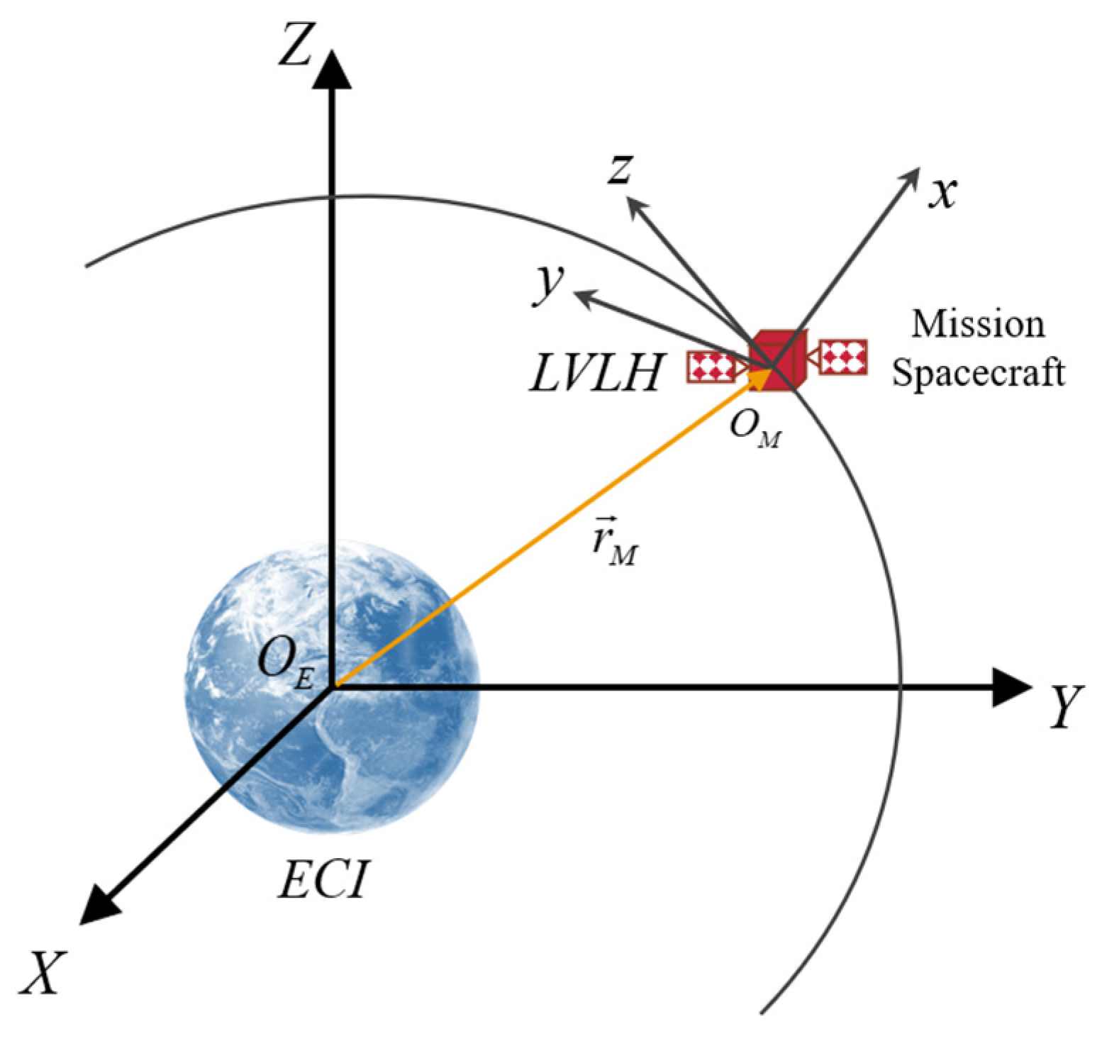
A local vertical local horizontal (LVLH) coordinate system
is established to describe the relative motion between spacecraft, using the center of mass of the mission spacecraft serving as the origin, as depicted in
Figure 1. The
plane corresponds to the orbital plane of the mission spacecraft, with the
axis pointing from the Earth’s center to spacecraft’s center of mass (
), the
axis aligning with the spacecraft’s angular momentum direction, and the
axis is determined by applying the right-hand rule.
Assuming that both the target spacecraft and the mission spacecraft operate in circular or near-circular orbits, the gravitational difference between the two spacecraft can be linearized. This assumption allows for the derivation of the equations governing the relative motion of the target spacecraft within the LVLH coordinate system of the task spacecraft:
In the equation, n denotes the orbital angular velocity of the spacecraft, while x, y, and z represent the position of the non-cooperative target’s center of mass within the LVLH coordinate system. Additionally, and represent the velocity of the non-cooperative target along the X and Y axes, respectively.
It should be noted that the in-plane variables x and y, along with the out-of-plane variable z, exhibit decoupled motion. This study primarily focuses on the relative motion within the orbital plane OXY of the reference spacecraft.
As a system of linear equations, the solution within the
OXY plane can be represented as follows:
where,
Additionally, the state of the non-cooperative target at the moment is represented in the LVLH coordinate system .
2.3. Definition of Non-Cooperative Target Intentions
The non-cooperative target’s intention is influenced by its relative motion patterns, which are influenced by orbital dynamics. Extensive research on relative motion patterns of spacecraft has been documented in the literature [
21,
22,
23]. Sabol et al. [
24] focused on the design of satellite formations and their temporal variation relationships, while Shasti et al. [
25] investigated the stability and control issues associated with relative configurations in satellite formations. Sun and Dang [
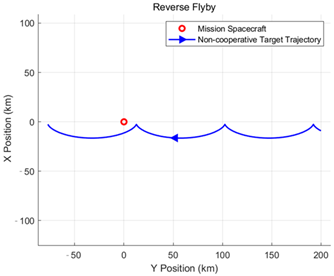
20] provided a detailed study of the formation conditions for droplet-like hovering configurations in the plane and classified non-cooperative target spacecraft intentions into 11 types. However, even though this classification method refines orbital behavior, certain behaviors may still correspond to the same intention in real-world scenarios. For example, both water droplet flybys and overhead flybys exhibit similar non-cooperative target behavior, where the target spacecraft passes over the task spacecraft in the +y to -y direction. Overly detailed intention types may lead to redundancy and inefficiency. Therefore, this paper optimizes and streamlines orbital behavior intentions for practical tasks based on the research of Sun and Dang [
20].
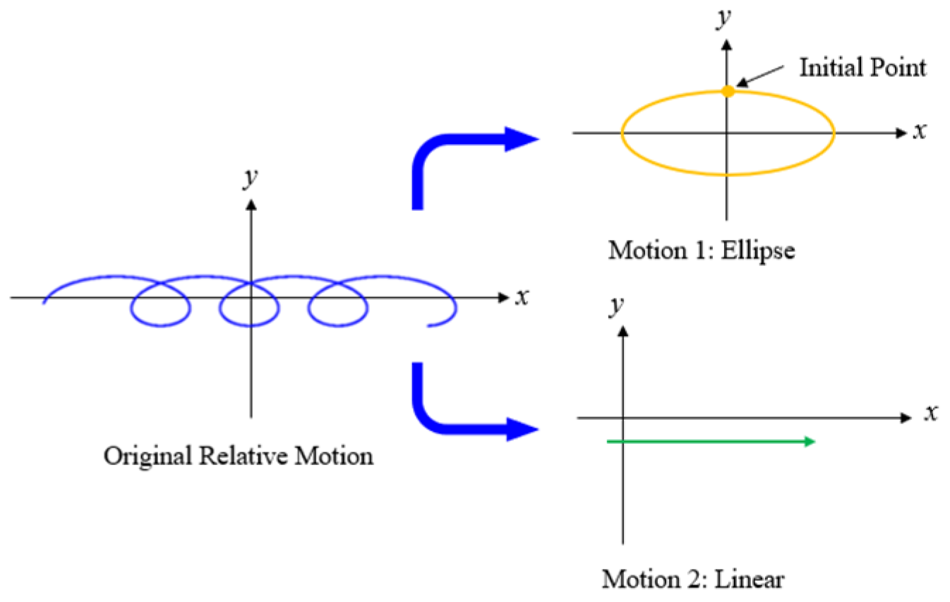
According to Equation (2), the relative motion within the orbital plane can be decomposed into a simple harmonic motion along the X-axis (motion 1) and a linear motion along the Y-axis (motion 2), as illustrated in the
Figure 2. Equations (5) and (6) for motions 1 and 2 are shown accordingly.
Motion 1 is characterized by circular motion along the ellipse, with X and Y components maintaining a constant 90° phase difference and a counterclockwise trajectory. In reference [
20], the intersection of motion 1 with the positive X-axis is identified as a feature point, which is used to represent different motion trajectories. In this study, the feature point is treated as the initial point of the relative motion; by varying this initial point, different relative motion trajectories of a non-cooperative space target can be obtained. The initial point exhibits the following properties:
Consequently, Equation (3) can be simplified to:
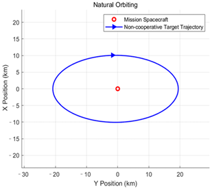
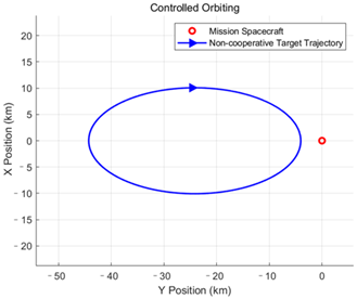
This paper classifies the intentions and orbital behaviors as follows. For the following intention, it primarily manifests as relative motion forms such as natural orbiting and controlled orbiting. For the approaching and distancing intention, two relative motion forms are identified: passing by and orbiting. The specific classification of orbital behavior intentions is shown in
Table 1.
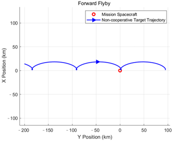
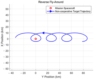
The following intention is mainly expressed through relative motion patterns, including natural orbiting and controlled orbiting. By contrast, approaching and distancing intentions encompass flyby and fly-around as two forms of relative motion, with the key difference being whether the motion creates an enclosing path around the mission spacecraft.
The target relative motion intent defined in this paper consists of six types: natural orbiting, controlled orbiting, forward fly-around, reverse fly-around, forward flyby, and reverse flyby. The specific definitions and formation conditions of these orbital behavior intents are presented in
Table 1.
2.4. Construction of the Intention Set Under Multiple Constraints
In practical operations, the relative orbital information of the non-cooperative target is acquired via the visual detection payloads of the mission spacecraft. Therefore, when constructing the intention set, it is essential to consider various environmental constraints affecting the relative orbital information. This paper specifically examines the impacts of illumination constraints and environmental errors.
- (1)
Illumination Constraints
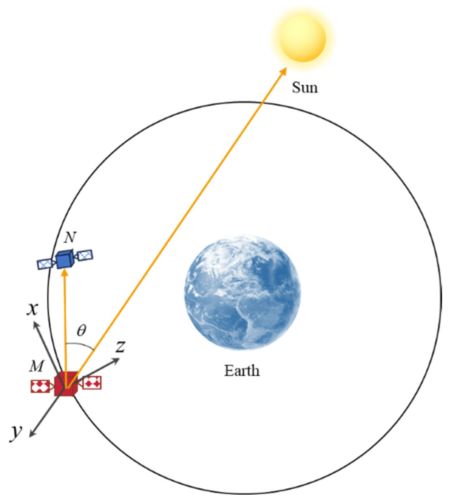
To describe the observation conditions of the task spacecraft for the non-cooperative target, the illumination azimuth angle
is shown in
Figure 3. This angle represents the orientation between the vector extending from the mission spacecraft
M to the non-cooperative target
N and the vector pointing from the
M to the sun within the LVLH coordinate system centered on
M. The expression of
is given by:
When is smaller than the constraint angle , the non-cooperative target N lies within the forward light angle of the mission spacecraft M, allowing it to conduct observations and obtain the corresponding orbital data.
- (2)
Payload Constraints
In practical scenarios, the payload’s operational range is limited, necessitating the determination of both the maximum detection distance
and the alarm distance
. In addition, the operating time of the payload and the spacecraft’s computer processing efficiency are constrained by the total satellite power, which can be represented by the capacity of the timing data
N and the interval time
. Under actual conditions, space disturbances such as atmospheric disturbances and space radiation may cause deviations between actual measurement values and ideal values. Hence, uncertainties and errors are considered, as shown in Equation (10):
where
represents the small deviations in the relative position and velocity of the orbital data.
3. Development of the Intention Recognition Model
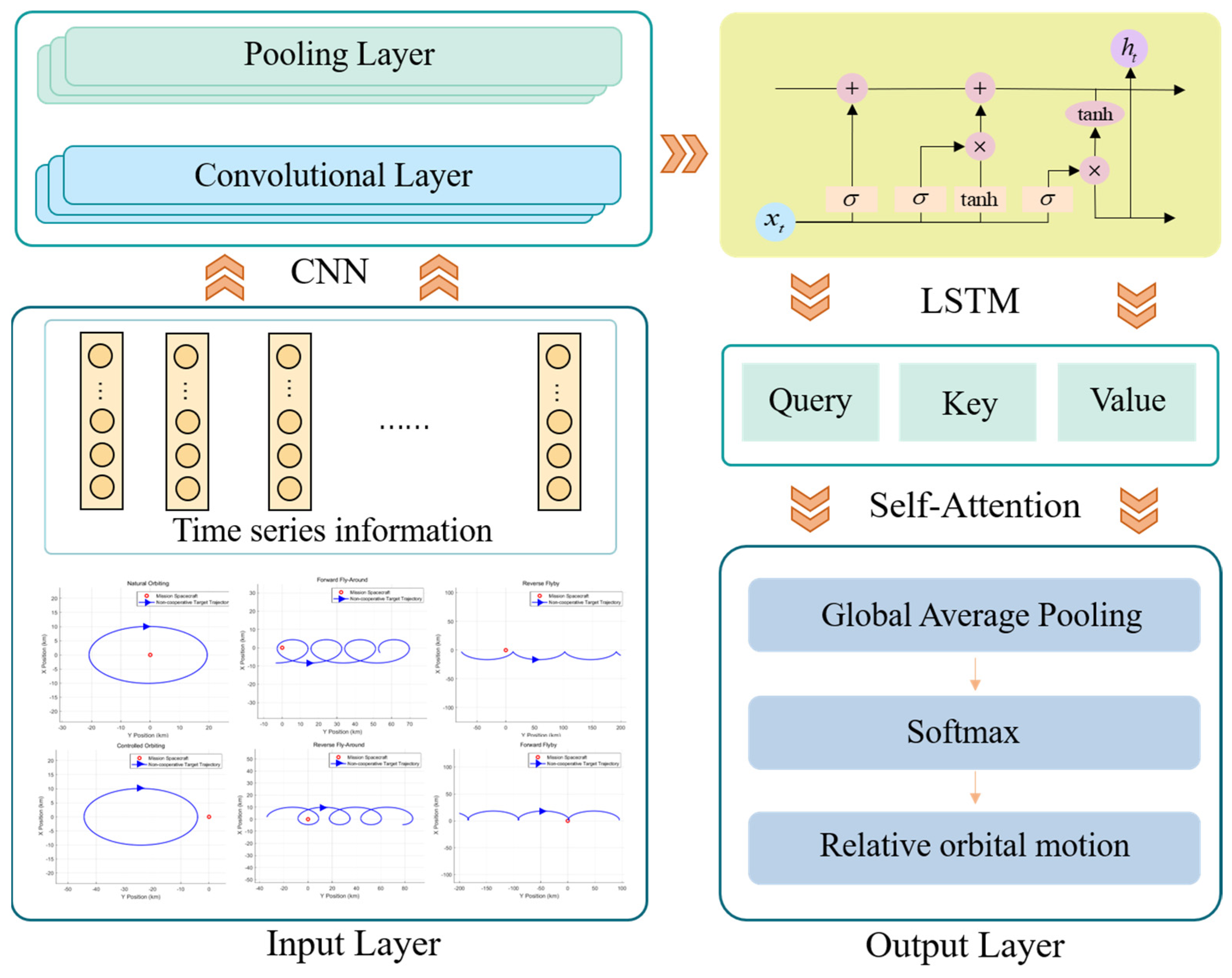
The network structure of the intention recognition method presented in this paper is illustrated in
Figure 4. It is composed of three layers: the input layer, the hidden layer, and the output layer. The hidden layer incorporates CNN, LSTM, and SA network structures. The detailed structure and functions of each layer are outlined below.
3.1. Input Layer
The input layer is responsible for preprocessing the collected feature data to generate feature, which are then directly processed by the subsequent layer. In this paper, the feature data are obtained through orbital simulations under multiple constraints, with specific details as follows.
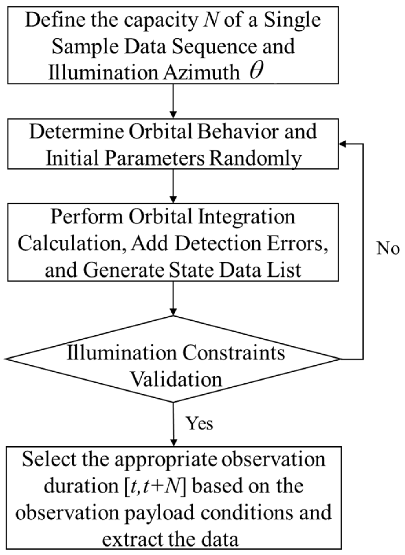
The intention and orbital behavior of the target spacecraft are randomly selected, while the initial conditions of the task spacecraft are specified. By applying numerical integration to Equation (8), the relative trajectory data of the target spacecraft over a given period are obtained. After generating the preliminary trajectory data, their compliance with the illumination conditions is assessed. A segment of trajectory data is then randomly selected within a specified time window
, ultimately forming a three-dimensional matrix of relative orbital behavior data.
Figure 5 illustrates the process of constructing a single sample instance.
To mitigate the impact of varying information scales across different features and enhance the model’s convergence efficiency, the original time series must be converted into dimensionless values with consistent intervals. In this study, a max–min linear transformation is applied to scale the data to the [0, 1] range. For the
x-dimensional feature data
, where
n represents the total number of data, the normalization formula is given as follows:
where
denotes the minimum value of the
x-dimensional feature,
denotes the maximum value,
corresponds to the data before normalization, and
refers to the normalized training data.
3.2. Hidden Layer
In the design of the hidden layer, this paper presents a deep learning model that combines a convolutional neural network (CNN), long short-term memory (LSTM) network, and a self-attention (SA) mechanism. By leveraging the strengths of each network structure, this hybrid model effectively extracts local features from time series data, captures long-term dependencies, and highlights crucial information, thereby enhancing the accuracy and robustness of non-cooperative target intention identification. The CNN layer is tasked with extracting spatial features, the LSTM layer is responsible for capturing long-term dependencies within time series data, and the self-attention mechanism emphasizes the most crucial segments of the sequence, mitigating information loss that commonly occurs in traditional methods when handling long time series data.
This integrated model exhibits superior performance in various complex environments, particularly in processing long time series data, where it achieves higher accuracy and better adaptability. The mechanisms of each layer are explained in detail below.
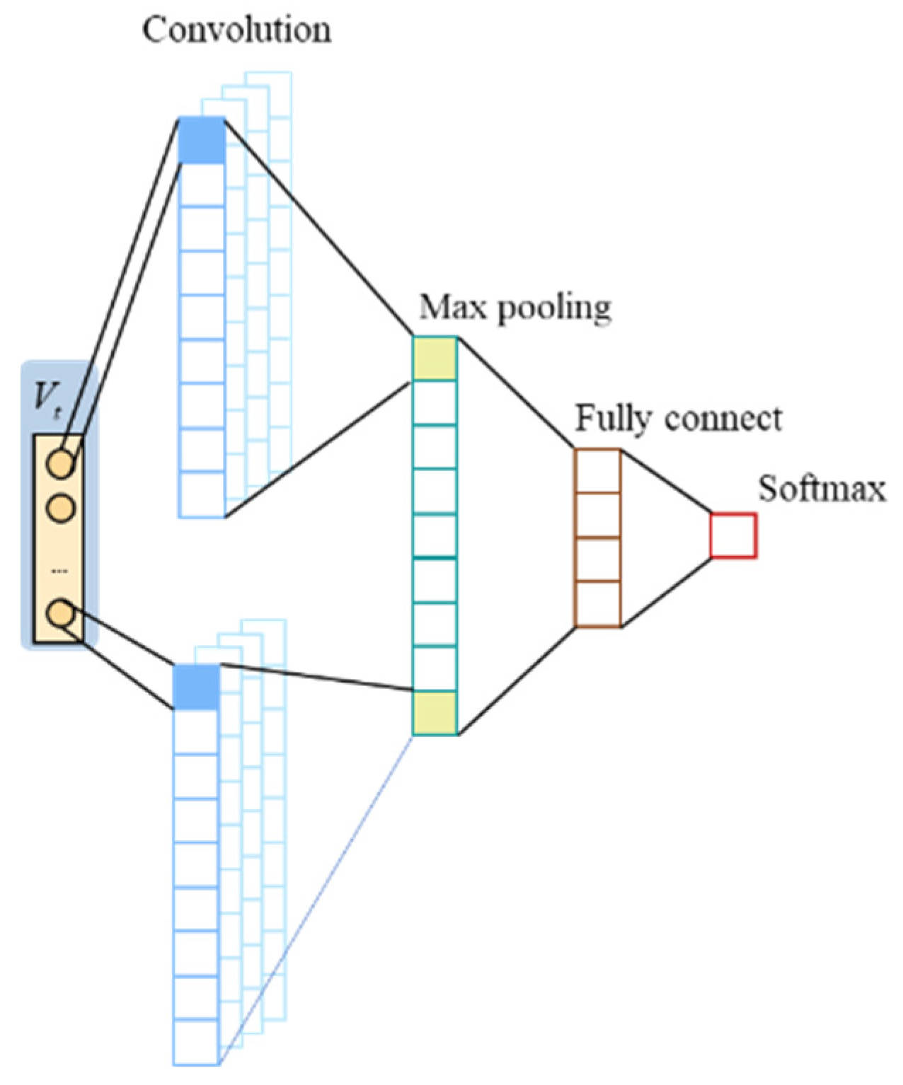
3.2.1. CNN Layer
A convolutional neural network (CNN) is a type of neural network engineered to automatically extract features from data, characterized by local connections, weight sharing, and spatial pooling. In this study, a CNN is used to extract local features from the input time series data. The network architecture comprises the convolutional, pooling, fully connected, and softmax layers, as shown in
Figure 6.
The convolution operation applies a sliding filter over the input data to extract key features. The computation of the convolutional layer can be expressed by the following equation:
where
represents the output feature of layer
l corresponding to index
i;
f is the nonlinear activation function of the network;
denotes the weight of the
i-th convolution kernel in layer
l;
is the convolution operation;
is the input to layer
l; and
represents the bias of the
i-th convolution kernel in layer
l.
The pooling layer, which follows the convolutional layer, reduces the dimensionality of the features while retaining crucial information. This compression helps to decrease computational costs and improves the overall efficiency of the model.
3.2.2. LSTM Layer
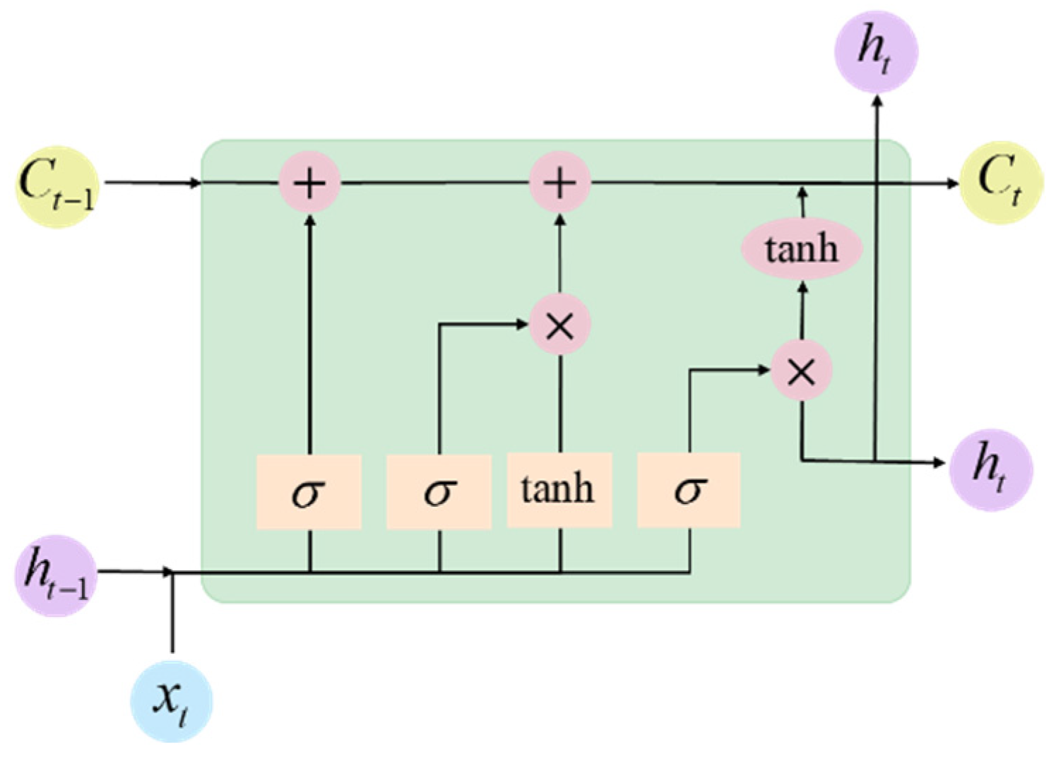
A long short-term memory (LSTM) network is a specialized form of recurrent neural network (RNN), with its architecture shown in
Figure 7. By introducing forget gates, input gates, and output gates to regulate the flow of information, LSTM addresses the vanishing gradient issue that can arise in traditional RNNs when learning long sequences.
The computation formula for the forget gate is given as follows:
In the formula, represents the activation function, while f denotes the output of the layer. and correspond to the previous and current unit states, respectively. , , , and are the weight matrices of the neural network. represents the “memory” of the neuron at time t, while denotes the input of the current cell.
LSTM effectively captures temporal features while preventing information loss in long time series data, thus providing a significant advantage in the long temporal sequence feature learning in this study.
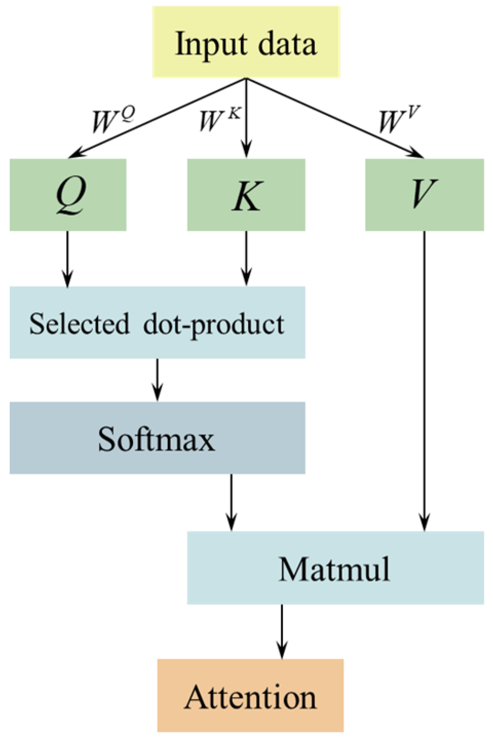
3.2.3. Self-Attention Layer
A self-attention (SA) mechanism models dependencies between any two positions in a sequence, addressing the information loss problem that may arise in long sequences when using traditional RNNs and LSTMs. In this study, the SA mechanism is primarily adopted to capture key features in long time series data and minimize reliance on external feature engineering. Its architecture is shown in
Figure 8.
The self-attention mechanism determines the relationships between each time step by calculating Query (
Q), Key (
K), and Value (
V) matrices from the input data, as shown in Equation (18):
where
,
, and
represent the three distinct weight matrices.
The self-attention calculation is expressed in Equation (19), in which
softmax() is the activation function:
where X is a dot-product attention calculation, which is more efficient by using matrix multiplication to calculate the correlation of each Query and Key Vector and sum them up. The softmax function maps the correlation of X and X in the range of [0, 1], which plays a normalization role. X is the square root of the key vector dimension and acts as a regulator to avoid the softmax function from entering the regions where it has extremely small gradients [
15].
This mechanism calculates the attention matrix to dynamically assign weights to each time step within the sequence, emphasizing the most important information. In this research, the self-attention mechanism is employed to process the long temporal trajectory data of non-cooperative targets, enabling more accurate capture of motion patterns, preventing information loss, and boosting the model’s capability to retain long-term dependencies, thereby significantly improving recognition accuracy.
3.3. Output Layer
In the model’s output layer, local features are first aggregated using an average pooling layer to form a global feature vector. The resulting data are then passed through a multi-class softmax function, which estimates the probability distribution over various intentions. Ultimately, the intention with the highest probability is chosen as the forecasted intention for the target. The computation formulas for the softmax function and the output layer are presented below:
In Equation (20), serves as the data fed into the softmax function. In Equation (21), W denotes the weight matrix of the dense layer to be trained, b is the corresponding bias term, and refers to the conceptual value associated with each intention in the output layer.
4. Experiments and Analysis
To evaluate the effectiveness of the proposed method, this section describes a series of simulations and analyses of the results. Initially, a dataset was constructed based on real-world conditions to verify the authenticity and reliability of the experiments. Subsequently, the model underwent training and validation processes. Finally, a comparison is made between the developed method and other models to confirm its advantages.
4.1. Dataset and Evaluation Metrics
Considering the large number of valuable spacecraft in high-altitude Earth orbits and the limited detection capabilities of ground-based sensors for these regions, there is an increasing need to identify the orbital behaviors of non-cooperative targets. Therefore, this study focuses on active proximity operations involving non-cooperative targets in high-altitude orbits. Multiple simulations were conducted with various target intentions, neglecting orbital perturbations, to obtain a range of relative motion patterns corresponding to each intention. The orbit of the mission spacecraft is defined as shown in
Table 2, with the following assumptions: the maximum detection range
of the spacecraft is 200 km, the minimum alarm distance
is 1 km, the continuous operating time of the detector (
N) is 60 s, and the spacecraft’s information processing interval
t is 1 s. A total of 60,000 sample data points were constructed, each consisting of 60 time steps, including the six intent types mentioned earlier, with 10,000 samples for each type. The dataset was divided into training, testing, and validation sets with a ratio of 8:1:1.
For model evaluation, several machine learning metrics were used, including accuracy, precision, recall, and the F1-score, with the corresponding calculation formulas outlined below:
In which TP denotes the instances where the model predicts positive, and the actual value is also positive; TN refers to the cases where the model predicts negative, and the actual value is negative; FP indicates the instances where the model predicts positive, but the actual value is negative; and FN refers to the instances where the model predicts negative, but the actual value is positive.
Accuracy indicates the ratio of correctly predicted samples by the model to the total number of samples, offering a comprehensive measure of the model’s predictive performance.
Precision represents the proportion of actual positive samples among the samples predicted as positive, assessing the accuracy of positive predictions. Recall represents the proportion of true positive samples identified by the model out of all actual positive samples, highlighting the model’s capacity to detect positive instances. The F1-score is the harmonic mean of precision and recall, with a higher score indicating better model performance.
4.2. Model Configuration
The dataset was generated through orbital simulations conducted in Matlab R2020a, while the neural network was implemented using Python 3.9 with the PyTorch 1.13.0 deep learning framework. Model training was conducted on a computer running Windows 11, equipped with an NVIDIA RTX 3060 GPU supported by CUDA 11.6 acceleration, and 48 GB of RAM.
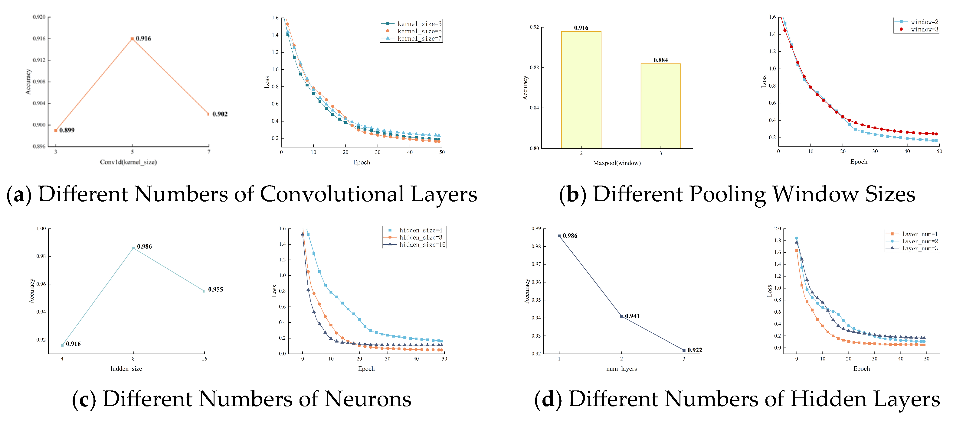
The experiment used cross-entropy as the loss function and Adam as the optimizer, evaluating different model structural parameters evaluated using the test set. Selecting appropriate hyperparameters is essential for optimizing the model and enhancing the efficiency of intention recognition. Based on the characteristics of the CNN-LSTM-SA model, the key hyperparameters selected included the convolutional kernel size, pooling layer window, number of neurons in the hidden layer, and number of hidden layers. A preliminary experiment was conducted with 50 iterations. The detailed parameter choices are presented in
Table 3, while the detailed experimental results are illustrated in
Figure 9.
First, the impact of the number of hidden layers on the model’s performance was examined. Three common kernel sizes—3, 5, and 7—were compared, with the pooling layer window set to 2, the number of neuron nodes fixed at 4, and the number of hidden layers set to 1 in experiments 1, 2, and 3. The results of this comparison are presented in
Figure 9a. When the convolution kernel sizes were 3, 5, and 7, the accuracies of the test set were 89.92%, 91.60%, and 90.20%, respectively. Among them, the model converged faster with a kernel size of 5, making it the optimal choice.
Subsequently, the effect of the pooling layer window on model performance was examined. Window sizes of 2 and 3 were tested, with the convolution kernel size set to 5, the number of neuron nodes fixed at 4, and the number of hidden layers set to 1 in experiments 2 and 4. The results of this comparison are presented in
Figure 9b. Increasing the pooling layer window to 3 degraded the model’s performance, reducing the test set accuracy to 88.40% and slowing down convergence. Therefore, a pooling layer window size of 2 was chosen.
Following this, the role of the number of neuron nodes in determining model efficiency was investigated. The number of neuron nodes selected was set to 4, 8, and 16, with the convolution kernel size set to 5, the pooling window set to 2, and the number of hidden layers set to 1 in experiments 2, 5, and 6. The results of the comparison are displayed in
Figure 9c. The accuracies of the test set were 91.60%, 98.62%, and 95.53%, respectively, when the number of neuron nodes was 4, 8, and 16. Among them, the model achieved the highest accuracy and the lowest loss when there were 8 neuron nodes, making it the optimal choice.
Lastly, the influence of hidden layer depth on the model’s accuracy and convergence speed was explored. The number of hidden layers was set to 1, 2, and 3, with the convolution kernel size set to 5, the pooling window set to 2, and the number of neuron nodes set to 8 in experiments 5, 7, and 8. The outcomes of the comparison are presented in
Figure 9d. When the number of hidden layers was increased to 2 or 3, the accuracy of the test set decreased to 94.15% and 92.23%, respectively, while the convergence speed also slowed down. Therefore, a single hidden layer was selected.
Based on the comparative experimental analysis, the model converged within 20 to 30 iterations, leading to the selection of 50 iterations as the optimal setting. The final model structure is presented in
Table 4.
4.3. Analysis of Model Results
4.3.1. Results and Analysis of the CNN-LSTM-SA Model
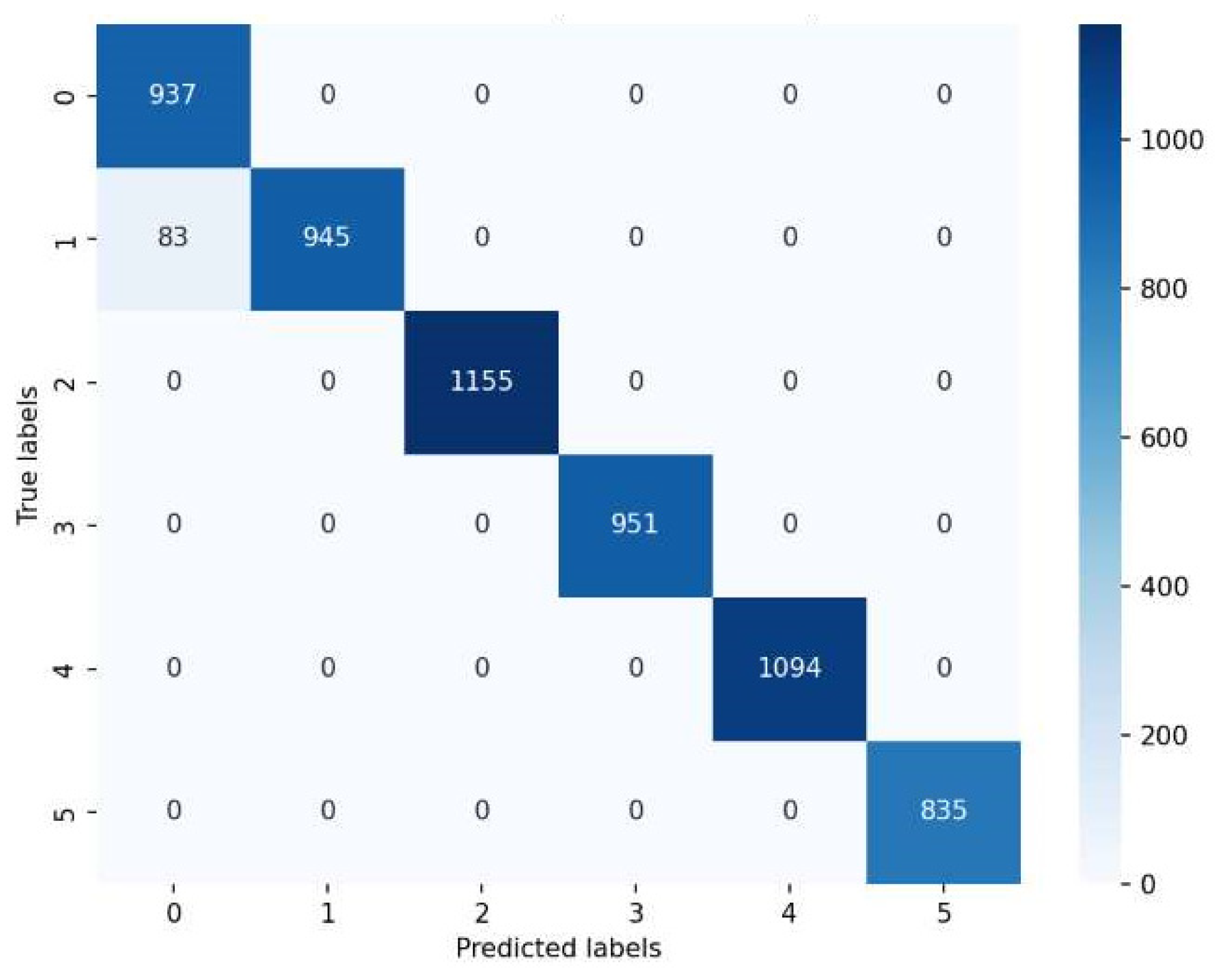
As illustrated in the figure, with an increasing number of iterations, the validation accuracy of the CNN-LSTM-SA model progressively improved, while the loss value decreased, eventually reaching convergence. The model attained an accuracy of 98.62%, with a final loss value of 0.049. A confusion matrix was created to visualize the recognition accuracy for each orbital behavior intention, aiding in the evaluation of the model’s reasoning, as shown in
Figure 11. In the figure, the predicted labels are displayed on the horizontal axis, while the true labels are represented on the vertical axis, and each diagonal element of the matrix indicates the number of correct classified instances. The figure demonstrates that the proposed intention recognition model achieved high accuracy across all intentions, confirming its reliability.
4.3.2. Performance Comparison Across Different Models
To further confirm the performance advantages of the proposed CNN-LSTM-SA model, a comparative evaluation was conducted on the same dataset with CNN, LSTM, CNN-LSTM, LSTM-SA, and the traditional support vector machine (SVM) model. The final results are presented in
Table 5.
To provide a more comprehensive evaluation of the model, computational complexity was introduced to assess both performance and efficiency. The final assessment considered each model’s computation time and test set accuracy after 50 iterations.
As presented in the table, the CNN-LSTM-SA model demonstrated higher accuracy than other models and a relatively simple structure. Compared to the traditional SVM model, the accuracy increased by 11.24%, and the recognition time was reduced by 162 s. In comparison to the individual CNN and LSTM models, the accuracy increased by 17.19% and 6.64%, respectively, with a reduction in completion time of 195 s and 144 s. In comparison to the CNN-LSTM model, the accuracy improved by 6.60%, accompanied by a slight increase in iteration time (by 17 s) due to the addition of the self-attention layer, which further enhanced feature learning. In comparison to LSTM-SA, the accuracy increased by 1.25%, and the recognition time was significantly reduced by 201 s, further emphasizing the effectiveness of the CNN layer in extracting key features.
These comparison experiments demonstrate that the model possesses strong input feature extraction capability, with the LSTM and self-attention mechanisms significantly enhancing intention recognition performance.


