Path Planning for Lunar Rovers in Dynamic Environments: An Autonomous Navigation Framework Enhanced by Digital Twin-Based A*-D3QN

Abstract

In lunar exploration missions, rovers must navigate multiple waypoints within strict time constraints while avoiding dynamic obstacles, demanding real-time, collision-free path planning. This paper proposes a digital twin-enhanced hierarchical planning method, A*-D3QN-Opt (A-Star-Dueling Double Deep Q-Network-Optimized). The framework combines the A* algorithm for global optimal paths in static environments with an improved D3QN (Dueling Double Deep Q-Network) for dynamic obstacle avoidance. A multi-dimensional reward function balances path efficiency, safety, energy, and time, while priority experience replay accelerates training convergence. A high-fidelity digital twin simulation environment integrates a YOLOv5-based multimodal perception system for real-time obstacle detection and distance estimation. Experimental validation across low-, medium-, and high-complexity scenarios demonstrates superior performance: the method achieves shorter paths, zero collisions in dynamic settings, and 30% faster convergence than baseline D3QN. Results confirm its ability to harmonize optimality, safety, and real-time adaptability under dynamic constraints, offering critical support for autonomous navigation in lunar missions like Chang’e and future deep space exploration, thereby reducing operational risks and enhancing mission efficiency.

1. Introduction

In contemporary space exploration, the Moon, as Earth’s sole natural satellite, holds paramount significance for scientific investigation. Lunar exploration not only facilitates resource development initiatives, such as the in situ utilization of lunar mineral resources to provide material support for deep space exploration and alleviate terrestrial resource constraints, but also drives technological innovation. The advancement of critical technologies, including lunar rover systems and path planning algorithms, exemplifies this dual-purpose development: these innovations not only fulfill mission-specific requirements for lunar exploration but also demonstrate significant potential to feed back into terrestrial engineering domains, thereby catalyzing industrial upgrading and technological transformation.

Lunar rover path planning stands as one of the critical technologies for lunar exploration missions. The objective of path planning is to identify an optimal trajectory from a starting point to a destination for mobile entities (e.g., robots, vehicles) in a given environment. An optimal path constitutes a core requirement for ensuring precise and efficient task execution by robotic systems [1]. In offline scenarios, path planning is typically implemented using predefined maps, where the environment is modeled as a grid-based maze and addressed through search algorithms such as A* [2] and Dijkstra [3]. Early research focused on enhancing traditional path planning algorithms. Tang et al. [4] proposed an improved A* algorithm integrated with environmental mapping techniques to optimize lunar rover path planning in rugged terrains, achieving significant reductions in path length and turning angles. Chen et al. [5] developed a Particle Swarm Optimization-based approach for autonomous waypoint selection, resolving inefficiencies in manual waypoint intervention and enabling efficient path exploration. Mamdapur et al. [6] constructed a lunar terrain model incorporating craters and steep slopes, compared the performance of Differential Evolution and Ant Colony Optimization in lunar rover path optimization, and analyzed the adaptability of these algorithms in complex topographies. However, the lunar surface environment presents significant challenges. Its complex terrain features include impact craters, steep slopes, and loose regolith; dynamic obstacles (e.g., moving meteoroids) and sudden environmental changes (e.g., abrupt local illumination shifts) demand real-time responsiveness; and potential path conflicts in multi-vehicle collaborative missions further exacerbate planning complexity. These challenges necessitate path planning algorithms that balance global optimality, dynamic adaptability, and multi-agent coordination. In recent years, researchers have proposed diverse local path planning methodologies, including the Artificial Potential Field (APF) [7], hybrid APF-Adaptive Dynamic Programming frameworks [8], Convolutional Neural Networks [9], and Reinforcement Learning (RL) [10], which have demonstrated efficacy in addressing obstacle avoidance in dynamic environments. Despite these advancements, existing planning systems in dynamic path planning environments often fail to respond promptly to unexpected scenarios (e.g., limited visibility).

Reinforcement Learning and deep reinforcement learning (DRL) have garnered significant attention in online path planning due to their adaptability to environmental changes and dynamic obstacles. As RL requires no predefined training data, it is particularly suited for scenarios demanding autonomous exploration. For instance, when training robots to perform specific tasks, the system incrementally adjusts action selection through trial and error: behaviors that increase reward signals are reinforced and executed more frequently. This learning paradigm mimics the conditioning of animals via reward-punishment mechanisms, ultimately enabling agents to autonomously optimize decision sequences in uncertain environments [11]. DRL integrates RL with deep learning, leveraging deep neural networks to enhance traditional RL algorithms (e.g., Q-learning), thereby overcoming performance limitations imposed by the curse of dimensionality. For example, in complex scenarios such as airports, mobile robots can utilize DRL to adapt to dynamically distributed pedestrians and sudden obstacles, achieving efficient navigation. This technology employs an end-to-end training mechanism that directly maps raw inputs to control policies, significantly enhancing the generalization capabilities of agents in open environments [12]. The Deep Q-Network (DQN) model proposed by Mnih et al. [13] represents a milestone in the integration of deep learning and RL, catalyzing advancements in RL methodologies. The applicability of DRL has gained widespread acceptance across multidisciplinary research communities. Yu et al. [14] demonstrated the application of safety-constrained DRL to end-to-end path planning for lunar rovers. Park et al. [15] implemented DRL for fault-tolerant motion planning of four-wheel dual-steering lunar rovers, though the long-term planning efficacy requires further validation. Lu et al. [16] developed a multi-rover collaborative path planning method combining DRL with Artificial Potential Field heuristics, addressing challenges such as obstacle avoidance across varying sizes and time-constrained target arrival. These innovative approaches have markedly improved the adaptability and responsiveness of lunar rover path planning strategies.

However, a more formidable challenge lies in the multidimensional characteristics of the lunar environment: motion uncertainties caused by lunar soil slippage, sensor drift induced by extreme temperature fluctuations, and emergent obstacles formed by dynamic meteorite impacts. These factors render pure deep reinforcement learning simulation training inadequate for ensuring algorithmic reliability in practical missions. For instance, while the LSTM-DRL framework developed by Hu et al. [17] achieved a 92% obstacle avoidance success rate in laboratory environments, its failure rate surged to 41% in unforeseen lunar shadow terrain, revealing a significant modeling gap between simulation and real-world scenarios. Digital twin (DT) technology provides critical support to address these limitations. Initially proposed by Professor Grieves [18], digital twin technology aims to create highly synchronized digital replicas of physical entities in virtual space. In aerospace applications, DT enables high-fidelity simulation environments for path planning in complex scenarios through real-time mapping of lunar rovers’ geometric characteristics, kinematic parameters, and environmental constraints. Specifically, digital twin models of lunar rovers incorporate not only static attributes like mechanical structures and sensor configurations but also dynamically simulate their motion postures, energy consumption, and obstacle interaction behaviors on lunar terrain. Through virtual-physical interactions, DT technology enables pre-validation of path planning strategies, thereby reducing operational risks and trial costs in real missions. With recent advancements in digital twin theory and technology, increasing research efforts have explored its applications in path planning. For example, Gan et al. [19] employed SPIS to construct 3D models simulating lunar rovers’ charging potential distributions in flat regions, shadowed areas, and near impact craters, analyzing solar incidence angles to mitigate threats posed by complex polar environments to electronic systems and sampling tasks. Yakubu et al. [20] developed a single-motor-driven wheel-legged lunar rover mobility system, addressing the high energy consumption and low fault tolerance of traditional multi-motor systems through DT simulations. Xia et al. [21] utilized DT to simulate system behaviors and predict process failures while integrating deep reinforcement learning into industrial control workflows, expanding system-level DT applications. Lee et al. [22] validated the potential of DT-driven DRL in robotic construction environments, demonstrating DRL’s adaptability in dynamic settings. These studies collectively indicate that the integration of digital twin technology with deep reinforcement learning can effectively bridge the gap between simulation and real-world implementation. These methodologies have proven effective in addressing obstacle avoidance challenges in dynamic environments.

Recent research has predominantly focused on navigation and obstacle avoidance in dynamic environments. Hu et al. [23] proposed a hierarchical framework combined with deep reinforcement learning for rapid path planning of planetary rovers in complex extraterrestrial environments, aiming to generate safe and efficient trajectories. Polykretis et al. [24] investigated mobile robot navigation in mapless environments by deploying a self-supervised cognitive map learner on edge devices, enabling autonomous environmental perception and cognitive map construction for navigation without prior maps. These studies have successfully accomplished navigation tasks through the development of DRL algorithms and their variants. Despite significant advancements in DRL, most approaches exhibit suboptimal performance in scenarios involving obstacles or multi-robot systems. For instance, Wei et al. [16] employed independent Q-learning, but their algorithm’s convergence speed degrades markedly as the number of robots increases, and it struggles to handle complex collaborative tasks requiring synchronized actions (e.g., scenarios demanding coordinated maneuvers). Their study explicitly notes that “an increase in robot count amplifies policy conflicts”, a critical concern given the potential for lunar rovers to obstruct one another. Pai et al. [25] discretized indoor environments into grids (e.g., 10 cm×10 cm), but such discretization may introduce collision risks when obstacles exhibit complex geometries (e.g., cylindrical shapes). R. Lowe et al. [26] introduced the Multi-Agent Deep Deterministic Policy Gradient (MADDPG) algorithm, significantly enhancing agent decision-making in mixed cooperative-competitive environments. While MADDPG demonstrates efficacy in certain scenarios, the authors also highlight its limitations in highly competitive or obstacle-dense environments (e.g., in “predator-prey” tasks, agents may fall into cyclic strategies, resulting in inefficiency). To address these challenges, this study proposes a novel lunar rover path planning framework, termed A*-D3QN-Opt. The research adopts the Deep Q-Network, a subfield of DRL, to resolve dynamic path planning problems by integrating an A*-algorithm-based static path planner with the D3QN algorithm. Here, A* generates initial paths in static environments, while D3QN optimizes trajectories and makes real-time decisions in dynamic settings. As an advanced DRL algorithm, D3QN combines the Double Q-Learning framework with a Dueling Network architecture, effectively mitigating traditional DQN limitations such as value overestimation and unstable convergence. Hasselt et al. [27] experimentally demonstrated that the dual-network structure reduces Q-value overestimation errors by 37%. By minimizing value function estimation bias through this architecture, D3QN enables rapid policy adaptation in dynamic obstacle scenarios (e.g., moving meteorites or other rovers). Furthermore, D3QN’s network design facilitates flexible integration of multimodal inputs, enhancing adaptability to complex perceptual environments. To further optimize the DRL model, this work enhances D3QN’s prioritized experience replay and reward function mechanisms. Additionally, the proposed method leverages a digital twin model to simulate lunar environments. Depth maps acquired from depth cameras and directional distance information from RGB cameras serve as model inputs, constructing a comprehensive state space to support agent decision-making and navigation.

The contributions of this paper are as follows:

1. Innovative Integration of the Two-Layer Path Planning Architecture: This study proposes a hierarchical path planning framework based on the A* algorithm and the improved D3QN algorithm. This architecture overcomes the limitations of traditional single-algorithm approaches by achieving efficient path planning in complex environments through a collaborative mechanism of static global planning and dynamic local adjustment. The A* algorithm is responsible for generating the global optimal path, addressing the low search efficiency of deep reinforcement learning in static environments. The D3QN algorithm, on the other hand, performs real-time adjustments to deal with dynamic obstacles and sudden environmental changes, enhancing the system’s adaptability. This layered design retains the global optimality of A* while leveraging the dynamic decision-making capability of deep reinforcement learning.

2. Multidimensional Optimization Strategy for the D3QN Algorithm: To address the issues of slow convergence and low sample utilization common in traditional deep reinforcement learning algorithms, this study optimizes the reward function and experience replay mechanism. A five-dimensional reward system was developed, incorporating path progress, obstacle avoidance, direction, energy consumption, and time penalties. This system effectively balances path efficiency and safety. Additionally, a priority sampling strategy based on TD-error is proposed, which dynamically adjusts the weight of experience samples, significantly improving the utilization efficiency of key experiences.

3. Improvement of the YOLOv5-DisNet Multi-Modal Perception System: To solve the challenges of target detection and distance estimation for the lunar rover in complex terrains, this study proposes a multi-modal perception approach integrating target detection and depth estimation. The traditional YOLOv3 is replaced by YOLOv5 [28], and obstacle detection is performed using the improved CSPDarknet53 backbone network and CIoU (Complete Intersection over Union) loss function. The data is then input into DisNet [29], where the target distance is precisely estimated by fusing object bounding box information with depth images. This information is provided as input to the path planning method for real-time obstacle avoidance.

Section 2 provides a detailed description of the proposed method, Section 3 presents the experimental results, and Section 4 concludes the study.

2. Methods

2.1. System Framework

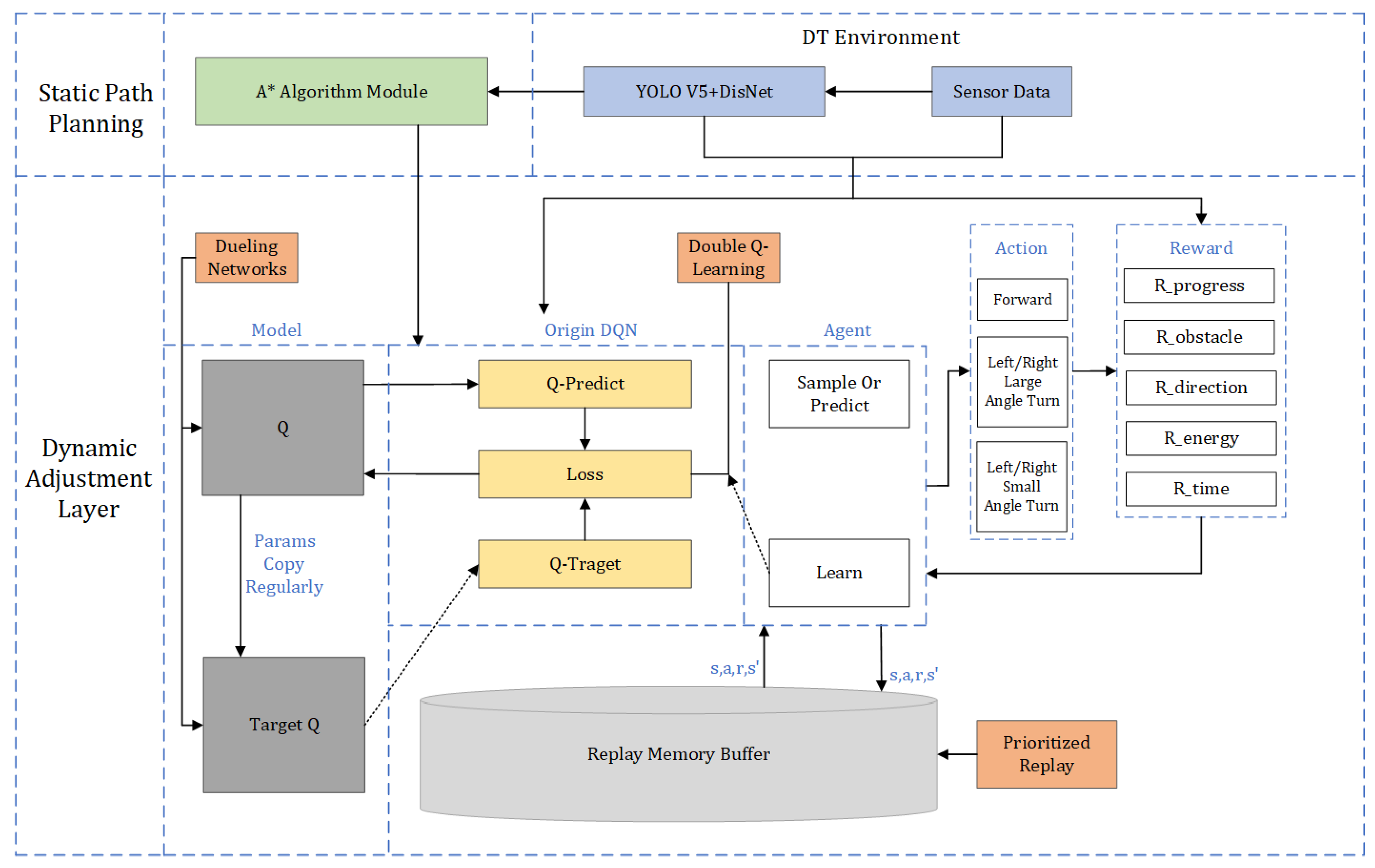
The lunar rover path planning system proposed in this paper is divided into a static global planning layer and a dynamic local adjustment layer, with the A* algorithm responsible for static path planning and the D3QN algorithm responsible for dynamic path optimization.

The initial module of the system is the static path planning, which employs the A* algorithm. This module is responsible for generating an initial global path in a static environment. The A* algorithm calculates the shortest path based on a predefined terrain map and avoids static obstacles. It lays the foundation for global path planning, ensuring the optimality of the path under ideal conditions.

Real-time sensor data, such as depth images and RGB images, provide crucial information regarding obstacles, terrain features, and distances. This data serves as input to both the static and dynamic planning modules. The proposed system integrates YOLOv5 with DisNet architecture [30], establishing a multimodal perception framework that synergizes target detection and depth estimation capabilities, enabling real-time environmental data acquisition.

The dynamic adjustment layer enhances the system’s responsiveness to environmental changes through D3QN (Dueling Double Deep Q-Network). This layer adjusts the path planning in real time based on sensor inputs. D3QN combines the dueling network architecture (which improves the stability of Q-value estimation) and double Q-learning (which reduces the bias caused by overestimation of Q-values) to handle dynamic obstacles. The agent module is responsible for decision-making. It selects actions based on the current state, which includes sensor data and terrain information. Actions include moving forward or turning at different angles (large or small turns). The agent learns from the environment through reinforcement learning to maximize long-term rewards. The Q-network predicts the Q-values for different possible actions, guiding the agent’s decision-making process. The target Q-network periodically updates its parameters to ensure learning stability. The Q-value is used to calculate both the Q-prediction (predicted Q-value) and the Q-target (target value computed through rewards and the next state). To optimize the learning process, a priority experience replay mechanism is used. This mechanism adjusts the sampling probability based on the temporal difference error (TD-error) of experiences, ensuring that important experiences are prioritized in the sampling process, thus accelerating learning. The system is designed with a detailed reward structure to guide the agent toward optimal path planning. The reward system consists of five components: path progress, obstacle avoidance, direction, energy consumption, and time consumption. Through these reward terms, the agent can balance path advancement, safe obstacle avoidance, and time efficiency. The replay memory buffer stores the agent’s past experiences (state, action, reward, and next state), which are used to train the Q-network. This allows the agent to learn from diverse experiences, improving decision-making quality. By combining static path planning and dynamic adjustment modules and employing deep reinforcement learning techniques, this architecture successfully addresses the challenges of autonomous navigation and obstacle avoidance for the lunar rover in complex terrains. The digital twin environment, advanced sensor data processing, and optimized reward functions and experience replay mechanisms enable efficient and safe path planning.

The system architecture of this paper is shown in Figure 1.

2.2. Digital Twin Environment Model Construction

In this section, we constructed a digital twin environment, including the lunar surface environment, lunar rover model, and sensor perspective views. To ensure the consistency between the digital twin environment and the real lunar surface, after injecting Gaussian noise into the simulation environment, the mean and standard deviation of the DisNet distance estimation error, as well as the mean and standard deviation of the target orientation angle deviation, meet the precision requirements for lunar rover obstacle avoidance decision-making. The root-mean-square (RMS) position tracking error and velocity error of dynamic obstacles are controlled within allowable ranges, ensuring the physical consistency of obstacle motion in the simulation environment, as shown in Figure 2.

2.2.1. Lunar Terrain Model

Based on lunar remote sensing data and elevation models, a three-dimensional lunar terrain grid is constructed. Terrain features (such as crater slopes and rock distributions) are generated using Gaussian random fields, with dynamic obstacles introduced to simulate the uncertainty of real-world environments. The terrain data is stored in a raster map format, with a spatial resolution of 0.1 m per pixel, ensuring the accuracy of path planning.

Gaussian noise with a mean of 0.1 m and a standard deviation of 0.05 m is injected into the simulation environment. Tests show that the root-mean-square error (RMSE) of distance estimation by DisNet is controlled within 0.08 m, and the standard deviation of target azimuth angle deviation does not exceed 0.5°. The position tracking error (RMSE) of dynamic obstacles is ≤0.15 m, and the velocity error is ≤0.05 m/s, meeting the precision requirements for lunar rover obstacle avoidance decisions.

Table 1. Quantitative parameters validation for digital twin environment.

Parameter	Value	Validation Method
Terrain Noise Mean	0.1 m	Gaussian Distribution Fitting of High-Fidelity Terrain Data
Distance Estimation Error (RMSE)	≤0.08 m	LiDAR Calibration Comparison
Azimuth Angle Deviation Standard Deviation	≤0.5°	Gyroscope-Vision Fusion Calibration
Dynamic Obstacle Position Error (RMSE)	≤0.15 m	Motion Capture System Tracking
Sensor End-to-End Latency	80 ms	High-Precision Timer Testing

demonstrates the validation of quantitative parameters for the digital twin environment.

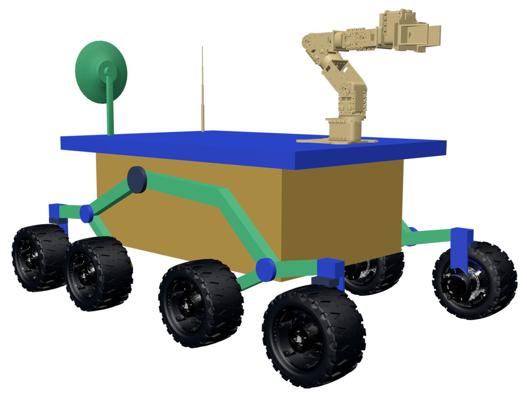
2.2.2. Lunar Rover Model

The modeling of the lunar rover includes both the three-dimensional rover model and the rover’s dynamic model. To study the rover’s driving performance on complex terrain, related research has explored the topic from multiple perspectives. Watanabe et al. [31] investigated the effect of wheel speed on the performance of a small two-wheeled lunar rover on lunar soil, including slip, sinkage, and power consumption. Through experiments, they tested the driving time, slip rate, power consumption, and sinkage at different wheel speeds and analyzed the relationship between wheel speed and ground reaction force. Chen et al. [32] established a forward and inverse kinematics model for an eight-wheeled torsion bar rocker-arm steering lunar rover, solving the relationship between rover body pose and wheel speed, providing a theoretical basis for motion control and autonomous navigation. Yang et al. [33] proposed a torque coordination control strategy, combining a wheel-ground interaction model to optimize the distribution of driving force for a six-wheeled rover on soft terrain, reducing energy consumption and improving mobility. Takehana et al. [34] analyzed the rutting characteristics of planetary rover gears on simulated lunar soil (Toyoura sand) through single-wheel test rigs and LiDAR scanning, quantifying the effect of load on rut depth and tilt. These studies collectively provide multidimensional theoretical and experimental foundations for the dynamic modeling and performance optimization of lunar rovers.

Based on the lunar rover’s geometric model and mechanical structure, a 3D physical model of the lunar rover is created. This model includes various components of the lunar rover, such as the wheels, rocker arms, and body. The kinematic model of the lunar rover describes the relationship between the wheel speed and the body speed. The lunar rover features an eight-wheel configuration with four steerable wheels and four fixed wheels, providing enhanced maneuverability on uneven terrain. Figure 3 shows the 3D model of the lunar rover. The kinematic model of the lunar rover can be expressed as follows:

$$\left\{\begin{array}{c}{V}_x={\displaystyle \frac{1}{2}}\left(V_{\omega 1}+V_{\omega 2}+V_{\omega 3}+V_{\omega 4}\right)\mathit{cos}\theta \\ V_y={\displaystyle \frac{1}{2}}\left(V_{\omega 1}-V_{\omega 2}+V_{\omega 3}-V_{\omega 4}\right)\mathit{sin}\theta \\ \omega ={\displaystyle \frac{1}{2L}}\left(V_{\omega 1}-V_{\omega 2}+V_{\omega 3}-V_{\omega 4}\right)\end{array}.\right.$$

(1)

Here, $V_x$ and $V_y$ are the velocities of the lunar rover in the x and y directions, $\omega$ is the angular velocity of the lunar rover, $V_{\omega i}$ is the linear velocity of the i-th wheel and its unit is m/s, $L$ is the wheelbase of the lunar rover unit: m, and $\theta$ is the heading angle of the lunar rover and its unit is rad.

The dynamics model of the lunar rover takes into account factors such as the rover’s mass, inertia, and the interaction forces between the wheels and the ground. The dynamics model can be described by the following system of equations:

$$\left\{\begin{array}{c}m{\ddot{V}}_x=F_x-mgsin\alpha \\ m{\ddot{V}}_y=F_y-mgcos\alpha sin\beta \\ I_z\ddot{\omega }=\tau \end{array}\right..$$

(2)

Here, $m$ is the mass of the lunar rover, and its unit is kg; $I_z$ is the moment of inertia of the lunar rover about the z-axis, and its unit is kg$·{\mathrm{m}}^2$; $F_x$ and $F_y$ are the driving forces of the lunar rover in the x and y directions; $\tau$ is the steering torque; $g$ is the gravitational acceleration on the lunar surface $g=1.62 \mathrm{m}/{\mathrm{m}}^2$; $\alpha$ is the pitch angle of the lunar rover, and its unit is rad; and $\beta$ is the roll angle of the lunar rover, and its unit is rad.

2.2.3. Sensor Simulation

The stereo vision principle is used to simulate the RGB-D camera, with key parameters including focal length, principal point coordinates, baseline distance, and resolution.

Parameters of the RGB-D camera: focal length f = 0.05 m, baseline distance B = 0.1 m, resolution 640 × 480. The sensor end-to-end latency is 80 ms (including 20 ms for image acquisition, 50 ms for YOLOv5 detection, and 10 ms for DisNet distance calculation), which meets the real-time control requirements. Table 1 demonstrates the validation of quantitative parameters for the digital twin environment.

The formula for generating depth images is as follows:

$$d\left(x,y\right)={\displaystyle \frac{B·f}{d_p\left(x,y\right)}},$$

(3)

where $d_p\left(x,y\right)$ is the disparity map (in pixels), $B$ is the baseline distance, and $f$ is the equivalent focal length (in meters).

RGB Image Generation: The texture mapping algorithm projects the material properties of the lunar terrain model onto the camera coordinate system to produce a color image. The output of YOLOv5 includes bounding box coordinates and class confidence. Based on the bounding box output from YOLOv5, DisNet calculates the target distance using the depth image. The depth image, RGB image, target orientation angle, and distance are integrated into the state vector $s_t$. The formula for generating the state vector is as follows:

$$s_t=\left[DepthMap,{\theta }_t,d_t\right],$$

(4)

where ${\theta }_t$ is the target orientation angle calculated from the image, with the unit of rad, and $d_t$ is the target distance computed by DisNet, with the unit of m.

With the above model, the digital twin environment can accurately simulate the sensor data collection process and provide reliable input for the path planning algorithm.

2.3. Path Planning Algorithm Based on D3QN

The path planning method proposed in this study adopts a two-tier architecture, dividing the path planning task into static global path planning and dynamic local path adjustment. This approach fully leverages the advantages of both the A* algorithm and the D3QN algorithm.

2.3.1. Static Path Planning Layer

The A* [2] algorithm is a classic heuristic search algorithm used to find the shortest path from the start point to the goal point in a graph. It combines the optimality of Dijkstra’s [3] algorithm with the efficiency of the greedy best-first search algorithm. The algorithm selects the next node to expand based on an evaluation function $f\left(n\right)$. The evaluation function $f\left(n\right)$ consists of two parts. The first part, the actual cost $g\left(n\right)$, represents the actual path cost from the start point to the current node. In lunar rover path planning, the actual cost can be calculated based on factors such as path length and terrain complexity. The second part is the heuristic estimate $h\left(n\right)$, which represents the estimated cost from the current node n to the goal node. To ensure the optimality of the A* algorithm, the heuristic function must satisfy the consistency (or monotonicity) condition. This means that for any node n and its neighboring node m, the following inequality must hold: $h\left(n\right)\le$ c(n,m) $+ h\left(m\right)$, where c(n,m) is the actual cost of moving from node n to node m. In this study, the Manhattan distance is used as the heuristic function, which calculates the sum of the horizontal and vertical distances between the current node and the goal node. It is simple and computationally efficient.

The core formula is as follows:

$$f\left(n\right)=g\left(n\right)+h\left(n\right),$$

where $g\left(n\right)$ represents the actual cost from the start point to the current node, and $h\left(n\right)$ is the heuristic function, which in this case is the Manhattan distance. The formula for the Manhattan distance is given by the following:

$$h\left(n\right)=\left|x_n\right.-\left.x_{goal}\right|+\left|y_n\right.-\left.y_{goal}\right|.$$

(5)

The coordinates of the goal node are ($x_{goal}$, $y_{goal}$), and the coordinates of the current node are ($x_n$, $y_n$).

2.3.2. Dynamic Path Adjustment Layer

Deep Q-Network is a reinforcement learning algorithm that combines deep neural networks with Q-learning. It uses neural networks to approximate the Q-value function, which addresses the limitations of traditional Q-learning when dealing with high-dimensional state spaces. However, DQN suffers from issues such as overestimating Q-values and slow convergence. The Duel Deep Q-Network effectively mitigates these issues by introducing a dueling network architecture and double Q-learning mechanism. In this study, the D3QN algorithm is used to handle path adjustment in dynamic environments, enabling intelligent decision-making based on real-time environmental and sensor data.

To further enhance the performance of the D3QN algorithm, this study improves its reward function and prioritized experience replay mechanism. The design of the reward function directly affects the learning behavior of the agent. A well-designed reward function can guide the agent to learn the optimal strategy more efficiently. The prioritized experience replay mechanism adjusts the sampling probability based on the importance of experience samples, allowing the network to make more effective use of valuable experiences, thus accelerating convergence.

The design of the state space needs to comprehensively consider the environmental information and task objectives of the lunar rover. In this study, multi-source sensor data is used to construct the state vector ${\mathrm{s}}_{\mathrm{t}}$, which includes depth images, target direction angles, and target distances. Depth images provide 3D geometric information about the lunar surface, helping the lunar rover identify the position and shape of obstacles. The target direction angle and target distance clarify the relative position of the lunar rover to the target point, offering directional guidance for path planning.

Depth images acquired from depth cameras typically exhibit high resolution and rich detail. To reduce computational load and enhance network training efficiency, the images undergo preprocessing steps. First, the image dimensions are resized to 80 × 64 pixels to align with the neural network’s input requirements. Subsequently, pixel values are normalized to the range [0, 1] to accelerate network convergence.

The target distance $d_t$ is calculated using an RGB camera integrated with the YOLOv5 object detection algorithm and the DisNet distance estimation algorithm, which provides distance information between the lunar rover and the target. The process begins by detecting the target’s bounding box ($x_{min}$,$y_{min}$,$x_{max}$,$y_{max}$) using YOLOv5. Based on the depth map and bounding box data, the actual distance dd is computed via DisNet using the formula $d={\displaystyle \frac{f·H}{h}}$, where H represents the predefined physical height of the target, and h denotes the height of the target’s bounding box in pixels.

The target orientation angle ${\theta }_t$, reflecting the required steering direction for the rover, is derived by calculating the angular difference between the rover’s current position and the target location. This angle is obtained by first localizing the target in the image coordinate system using RGB data. The camera’s intrinsic parameters—focal length f and principal point $(c_x,c_y$)—are then applied to convert the target’s pixel coordinates into its relative azimuth angle. Finally, the angle value is normalized to the range [−π, π].

The speed actions ${\mathrm{v}}_1=0$.2 m/s and ${\mathrm{v}}_2=0$.4 m/s represent low-speed and high-speed movement, respectively. Under different terrain and environmental conditions, the lunar rover can choose the appropriate speed to improve driving efficiency and safety.

The steering actions ${\mathrm{w}}_1=\mathsf{\pi }$/4, ${\mathrm{w}}_2=\mathsf{\pi }$/8, ${\mathrm{w}}_3=$0, ${\mathrm{w}}_4=-\mathsf{\pi }$/8, and ${\mathrm{w}}_5=-\mathsf{\pi }$/4 represent a large left turn, a small left turn, moving straight, a small right turn, and a large right turn, respectively. Through these steering actions, the lunar rover can flexibly adjust its driving direction.

The action space comprises seven discrete actions combining velocity and steering angle configurations, defined as follows:

Low-speed sharp left turn: velocity = 0.2 m/s, steering angle = π/4.

Low-speed gentle left turn: velocity = 0.2 m/s, steering angle = π/8.

Low-speed straight motion: velocity = 0.2 m/s, steering angle = 0.

Low-speed gentle right turn: velocity = 0.2 m/s, steering angle = π/8.

Low-speed sharp right turn: velocity = 0.2 m/s, steering angle = π/4.

High-speed straight motion: velocity = 0.4 m/s, steering angle = 0.

Emergency stop: velocity = 0 m/s, activated for obstacle avoidance or mission termination.

For action selection, an ε-greedy strategy is implemented with an initial exploration rate (ε) of 0.5, which decays exponentially to a minimum value of 0.05 at a decay rate of 0.99. During later training phases, when the policy transitions toward exploitation, the strategy prioritizes selecting actions with the highest Q-values.

2.3.3. Improved Reward Function

The design of the reward function is a critical component of reinforcement learning, as it directly influences the agent’s learning performance and behavioral strategy. In this study, the principle for designing the composite reward function is to encourage the lunar rover to move towards the target while avoiding collisions with obstacles, improving driving efficiency and safety. By considering multiple factors, including path progress, obstacle avoidance, driving direction, energy consumption, and time consumption, a comprehensive reward function is designed.

In lunar rover path planning, the improved composite reward function $R=R_{progress}+R_{obstacle}+R_{direction}+R_{energy}+R_{time}$ guides the agent to learn the optimal strategy from multiple dimensions.

Path Progress Reward R_{progress}: This reward term is used to encourage the lunar rover to move towards the target. By comparing the current position with the previous position’s distance to the target, the path progress reward is calculated. If the rover is closer to the target, a positive reward is given; if it is farther from the target, a negative reward is given. The magnitude of the reward is proportional to the change in distance, allowing the rover to move towards the target more quickly. The calculation method is as follows:

$$R_{progress}={\displaystyle \frac{d_{prev}-d_{current}}{d_{prev}}}\times 10.$$

(6)

$d_{prev}$ is the distance from the lunar rover to the target point at the previous time step, and $d_{current}$ is the current distance to the target point. If $d_{current}$ < $d_{prev}$, it indicates that the lunar rover is approaching the target, and $R_{progress}$ will be a positive reward. The larger the difference, the higher the reward. If the distance has not decreased or even increased, the reward will be negative, prompting the agent to adjust its strategy.

Obstacle Avoidance Reward R_{obstacle}: To prevent the lunar rover from colliding with obstacles, an obstacle avoidance reward term is designed. The distance to obstacles is detected using depth images and sensor data, and the weighted sum of obstacle distances in 8 directions is computed to obtain the obstacle avoidance reward. If an obstacle is detected to be nearby, a larger negative reward is given, encouraging the lunar rover to adjust its direction in time. The calculation method is as follows:

$$R_{obstacle}=-{\sum }_{i=1}^8{\displaystyle \frac{d_i}{d_{max}}}\times 5.$$

(7)

$d_i$ represents the distance to obstacles detected in the 8 directions around the lunar rover (obtained through depth cameras and other sensors), and $d_{max}$ is the predefined maximum detection distance. The closer the obstacle is (the smaller $d_i$ is), the smaller the ${\displaystyle \frac{d_i}{d_{max}}}$ value becomes, and after applying the negative sign, the absolute value of $R_{obstacle}$ increases. This results in a stronger negative reward, which strongly penalizes behaviors that bring the rover closer to obstacles, forcing the agent to actively avoid them.

Direction reward R_{direction}: The direction reward is designed to guide the lunar rover towards the target direction. By calculating the cosine value of the angle between the current travel direction and the target direction, the direction reward is obtained. When the angle is small, the cosine value approaches 1, and a positive reward is given; when the angle is large, the cosine value approaches −1, and a negative reward is given. This ensures that the lunar rover moves more accurately towards the target direction. The calculation is as follows:

$$R_{direction}=\mathit{cos}\left({\theta }_t\right) \times 3$$

(8)

${\theta }_t$ is the angle between the lunar rover’s current travel direction and the target direction. The value of $\mathit{cos}\left({\theta }_t\right)$ ranges from [−1, 1], where the smaller the angle (the more accurate the direction), the closer $\mathit{cos}\left({\theta }_t\right)$ is to 1, resulting in a higher reward. The larger the angle, the lower the reward, or even negative, which encourages the agent to adjust its direction to align with the target.

Energy Consumption Reward R_{energy}: Considering the limited energy of the lunar rover, an energy consumption reward term is designed. The reward is calculated by comparing the difference between the current travel speed and the optimal speed. If the travel speed deviates significantly from the optimal speed, a negative reward is given, encouraging the lunar rover to operate in a more energy-efficient manner. The calculation is as follows:

$$R_{energy}=-{\displaystyle \frac{v_t-v_{optimal}}{v_{max}}}\times 2.$$

(9)

$v_t$ is the current travel speed, $v_{optimal}$ is the preset optimal energy-efficient speed, and $v_{max}$ is the maximum speed of the lunar rover. The larger the deviation between $v_t$ and $v_{optimal}$, the greater the absolute value of ${\displaystyle \frac{v_t-v_{optimal}}{v_{max}}}$, resulting in a more significant negative reward. This encourages the agent to travel at a reasonable speed, thereby conserving energy.

Time penalty R_{time}: To improve the efficiency of path planning, a time penalty term is designed. As time increases, a negative reward is given, encouraging the lunar rover to reach the target point as quickly as possible and minimize unnecessary time consumption. The calculation is as follows:

$$R_{time}=-0.01 \times t.$$

(10)

$t$ is the total time steps from the starting point to the current time. As time increases, the negative penalty $R_{time}$ accumulates, motivating the agent to plan the path efficiently, reduce time consumption, and improve task execution efficiency.

Through the collaborative effect of the five reward components, the agent (D3QN) can achieve a balance between path progress, obstacle avoidance, direction, energy consumption, and time efficiency, learning an efficient path planning strategy that adapts to the complex lunar environment.

2.3.4. Prioritized Experience Replay Mechanism

The traditional experience replay mechanism randomly samples experiences from the experience pool for training. This approach may cause the network to learn from some less important experiences while neglecting critical ones. The prioritized experience replay mechanism adjusts the sampling probability based on the importance of experience samples, enabling the network to more effectively learn from valuable experiences. In this study, the temporal difference (TD) error ${\delta }_i$ is used to measure the importance of experience samples. A larger TD error indicates that the experience sample is more valuable for updating the network.

TD-error Calculation: The TD-error ${\delta }_i$ represents the difference between the current estimated Q-value and the target Q-value. The calculation formula is as follows:

$${\delta }_i=r+\gamma \mathit{max}{Q}^{\prime }\left(s_{t+1},a_{t+1}\right)-Q\left(s_t,a_t\right),$$

(11)

where r is the reward at the current time step, $\gamma$ is the discount factor, $Q^{\prime }\left(s_{t+1},a_{t+1}\right)$ target is the maximum Q-value of the next state estimated by the target network, and $Q\left(s_t,a_t\right)$ is the Q-value estimated by the current network.

To avoid sampling issues caused by a TD-error of 0, a small positive value $ϵ$ is added to the TD-error, resulting in the priority ${\psi }_i$.

$${\psi }_i=\left|{\delta }_i\right|+ϵ.$$

(12)

Sampling probability calculation: The sampling probability $P(i$) of an experience sample is directly proportional to its priority ${\psi }_i$, and is calculated as follows:

$$P\left(i\right)={\displaystyle \frac{{{\psi }_i}^{\alpha }}{{\sum }_j{{\psi }_j}^{\alpha }}},$$

(13)

where $\alpha$ is the parameter that controls the priority level, with $\alpha$ = 0 indicating random sampling and $\alpha$ = 1 indicating sampling entirely based on priority.

During the training process, the experience replay buffer (ERB) is used in the following stages. When the agent interacts with the environment and executes an action, it collects relevant state information, the action taken, the reward obtained, and the next state, which are stored in the ERB. Specifically, after each action executed by the agent in the environment, a tuple (current state $s_t$, action $a_t$, reward r, next state $s_{t+1}$, and termination flag) is stored in the ERB. This process continues from the start to the end of training, recording all historical experiences of the agent-environment interactions. In each training cycle, a mini-batch of experience samples is randomly sampled from the ERB to train the Q-network. These samples update the network’s weights and biases to improve the agent’s policy. For example, in the early training phase, once the ERB accumulates sufficient samples, 64 samples are randomly drawn for training in each cycle, enabling the agent to learn from past experiences and gradually enhance decision-making.

The prioritized experience replay (PER) mechanism introduces special usage of ERB. Experience samples are assigned priorities based on the TD error, i.e., the difference between the current predicted Q-value and the target Q-value. A larger TD error indicates higher importance of the sample, hence a higher priority. Sampling from ERB is performed according to these priorities rather than randomly, with high-priority samples having a higher selection probability to ensure the agent learns more from critical experiences. As training progresses, sample priorities are dynamically updated based on new TD errors. For instance, after each training cycle, the TD errors of sampled experiences are recalculated to update their priorities, allowing the ERB to continuously reflect the latest learning focus and facilitate more efficient learning.

2.4. Environmental Perception and Data Processing

The depth images are obtained using an RGB-D camera and provide 3D geometric information about surrounding objects. In this study, in addition to using the current depth image, the previous three depth images are also used to acquire 3D information about surrounding objects. Considering computational costs, all depth images are resized to 80×64. While the depth images provide essential information for the mobile robot to avoid both static and dynamic obstacles under the control of the agent, additional inputs are necessary for the robot to reach a given target. The first of these additional inputs is the direction of the target. In addition to providing this information as extra input to the fully connected layer of the model, it is also utilized within the reward-punishment system structure. The target direction information is obtained using the RGB camera and the OpenCV library in this study.

In the autonomous path planning task of the lunar rover, target detection and distance calculation are among the key technologies for achieving autonomous navigation and obstacle avoidance. In addition to the direction of the target, another additional input to the model is the target’s distance. First, the target must be detected to obtain the distance. A YOLOv3-based DisNet is used to detect the target and estimate the distance [35]. DisNet is a deep neural network designed to extract depth information from images and estimate the distance to the target. The main goal of DisNet is to calculate the actual distance between the target object and the lunar rover based on the target’s bounding box in the image. In the path planning of the lunar rover, accurate distance estimation is crucial for determining path selection and obstacle avoidance effectiveness. YOLOv5, using the PyTorch (version 1.12.1) framework, provides higher detection accuracy and speed [36]. Compared to YOLOv3, YOLOv5 offers improved detection precision and speed and performs better in complex scenes, providing more accurate target bounding boxes. Specifically, YOLOv5 utilizes an improved neural network architecture, achieving a better balance between processing speed and accuracy. The bounding box coordinates and the confidence scores for the target classes output by the model have been optimized, allowing for more precise target localization, making YOLOv5 particularly suitable for autonomous navigation of lunar rovers in complex environments. Furthermore, in the same lunar simulation scenario, we compared the performance of YOLOv3 and YOLOv5 using the mean average precision (mAP) at an Intersection over Union (IoU) threshold of 0.5. The dataset comprised 2000 annotated RGB images (synthetic + real lunar surface data), including lunar terrain obstacles such as craters and rocks. The results showed that YOLOv3 achieved an mAP of 72.3%, while YOLOv5 achieved 83.1%, representing a 15% relative improvement. The training data we use is a 1:1 mixture of real and simulation-generated data and is labeled using labeling. Therefore, in this study, the target detection implementation code was modified to adopt the YOLOv5 output results, and the target detection results were parsed based on YOLOv5’s optimizations. These results were then used as input for DisNet to estimate the distance. DisNet takes the target bounding boxes output by YOLOv5 and depth images as inputs. Its core task is to calculate the actual distance $d_t$ between the target and the lunar rover based on the target’s size in the image and camera parameters through Equation (7). The feature calculation module is responsible for fusing multi-source data to integrate the feature vector $s_t$, including depth images, distance calculation $d_t$, and direction angle ${\theta }_t$. Finally, this information is provided as input data to the Deep Q-Network model, ultimately achieving path planning for the lunar rover. Figure 4 illustrates the environmental perception and data processing system architecture.

In this study, YOLOv5 is used for real-time detection of objects (obstacles and target locations) around the lunar rover, while DisNet is employed to calculate the actual distance between the target and the rover, providing more accurate spatial perception information. In the digital twin environment, DisNet’s distance estimation results were validated against LiDAR measurements as ground truth, with the error metric being relative error (i.e., the difference between DisNet’s estimation and LiDAR measurements). Among 1500 test samples (distance range 1–20 m), 95% of errors fell within ±5% (with a maximum error of 6.2% at 20 m). Within the typical operational range of the lunar rover (1–10 m), the relative error is less than 5%. YOLOv5 takes pre-processed RGB images as input and outputs the bounding box coordinates and class confidence for each detected target object. Specifically, the output includes the bounding box coordinates ${\widehat{b}}_{ij}$:($x_{min}$,$y_{min}$,$x_{max}$,$y_{max}$) for the target, as shown in the following Formula (14), and the class confidence ${\widehat{p}}_{ij}$ for each target, as shown in Formula (15).

$${\widehat{p}}_{ij}=\sigma (con{f}_{ij})\times 1_{[i=c]}.$$

(14)

$${\widehat{b}}_{ij}=\sigma \left(b_{ij}\right).$$

(15)

${\widehat{p}}_{ij}$ is the confidence of the i class target in the j detection box, ${\widehat{b}}_{ij}$ is the coordinates of the target bounding box processed by the Sigmoid function, where σ represents the Sigmoid function, and ${conf}_{ij}$ is the confidence of the target.

YOLOv5 outputs the bounding box coordinates and class information of the target objects, while DisNet combines this information with the depth data of the image. Each detection box output by YOLOv5 not only contains the class of the target but also provides its position in the image. Therefore, DisNet estimates the depth of the target objects using the bounding box information provided by YOLOv5. The input channels of the DisNet network receive the target areas output by YOLOv5 and further extract depth features through convolutional layers.

In this study, DisNet estimates the target distance using the depth map, with the calculation formula given by Equation (16).

$$d={\displaystyle \frac{f·H}{h}}.$$

(16)

$d$ is the actual distance of the target object, $f$ is the focal length of the camera, $H$ is the actual height of the target object, and $h$ is the image height of the target obtained through DisNet, which corresponds to the height of the bounding box.

The feature calculation module constructs the feature vector $s_t$ by combining the actual target distance $d_t$ calculated by DisNet, the target direction angle ${\theta }_t$ parsed from the image, and the processed depth image. The formula is shown as Equation (17).

$$s_t=\left[DepthMap,{\theta }_t,d_t\right],$$

(17)

where ${\theta }_t$ is the target orientation angle calculated from the image, and $d_t$ is the target distance calculated by DisNet.

By combining YOLOv5 and DisNet, the lunar rover is capable of precise target detection and distance calculation.

In summary, for depth images, the input layer of the D3QN neural network architecture accepts an 80 × 64 × 4 depth map sequence. The convolutional layers are structured as follows: Layer 1: 32 8 × 8 convolutional kernels with a stride of 4, activated by ReLU. Layer 2: 64 4 × 4 convolutional kernels with a stride of 2, activated by ReLU. Layer 3: 64 3 × 3 convolutional kernels with a stride of 1, activated by ReLU. Depth images are processed through these three CNN layers to automatically extract spatial features, such as edges, shapes, and relative positions of obstacles. The features extracted by the convolutional layers are flattened and concatenated with two additional features: target orientation angle ${\theta }_t$ and target distance $d_t$, forming a comprehensive feature vector.

The fused feature vector is fed into a 512-dimensional fully connected layer, which further processes and integrates the features to enable the network to learn complex relationships among them. The output of the fully connected layer branches into two streams: the Value Stream and the Advantage Stream. The Value Stream evaluates the quality of the current state, while the Advantage Stream assesses the relative advantages of different actions in the current state. The output layer consists of seven neurons corresponding to the Q-values of seven discrete actions. Each neuron’s output represents the expected return of the corresponding action in the current state. The lunar rover selects the optimal action (e.g., forward movement or steering) based on these Q-values to achieve efficient path planning.

3. Results and Analysis

3.1. Experimental Setup

In the experimental study, nine training sessions were conducted using three different methods across three distinct scenarios. The simulation environment, along with the average Q-value and cumulative reward per episode, was used as a metric to evaluate the training process. We used the Adam optimizer with a learning rate of 0.00025 for DQN training. During the training process, the ε-greedy decreased from 1 to its minimum value of 0.05, with a decay rate of 0.99. The weight parameter α equals 1. The experience replay memory size was set to 250,000, and 64 mini-batches were randomly sampled from the experience replay buffer for each training epoch. All parameters used are presented in

Table 2. Values of hyperparameters in the conducted experiments.

Hyperparameter	Value	Explanation
Action space size	7	Contains 7 discrete actions, such as low-speed steering and high-speed straight movement
ε	0.5	Initial exploration rate using ε-greedy strategy
${\epsilon }_{min}$	0.05	Lower bound for exploration rate decay
Exploration rate decay factor	0.99	Exponential decay factor to reach the minimum value
Prioritized experience replay buffer size	250,000	Maximum number of experiences stored
α	1	Controls the intensity of sampling priority; α = 1 means sampling fully based on priority
random seed	42	Normally, a random seed is employed in random number generation to ensure that each experiment is reproducible.
Mini-batch size	64	Number of samples per training batch
Maximum training episodes	1000	Total number of training rounds
Time-out steps	500	Maximum steps per episode; reset if exceeded
Learning rate	0.00025	Learning rate for the Adam optimizer
R_progress weight	10	Proportional coefficient in formula (6), encouraging approach to the target
R_obstacle weight	−5	Weighted sum coefficient in formula (7), punishing proximity to obstacles
R_direction weight	3	Cosine value coefficient in formula (8), guiding orientation toward the target
R_energy weight	−2	Velocity deviation coefficient in formula (9), punishing abnormal energy consumption
R_time weight	−0.01	Time step coefficient in formula (10), punishing excessive time consumption
Angular velocity of moving obstacles	0.35 rad/s	Obstacles move clockwise at 0.35 rad/s in stage 3

.

The complexity of the three different scenarios is classified into low complexity, medium complexity, and high complexity. As shown in Figure 5, the training environment for the lunar rover is a 10 m x 10 m square area with three stage configurations (Figure 5). In the first stage, there are no obstacles (Figure 5a); in the second stage, there are four static cylindrical obstacles (Figure 5b); and in the third stage, there are four obstacles moving along a circular trajectory (Figure 5c). The second stage is more challenging than the first, and the third stage, due to the presence of dynamic obstacles, is the most challenging. The obstacles move in a clockwise direction with an angular velocity of 0.35 rad/s.

In this environment, the lunar rover starts from the origin (0,0) and navigates toward the target. When it collides with a wall or an obstacle, the environment is reset by the agent, and the lunar rover is repositioned to the starting point. This marks the end of an episode. Otherwise, whenever the lunar rover reaches the target, the environment randomly places a new target, and navigation begins again. The lunar rover collects rewards by executing actions determined by the policy at each step until a timeout occurs.

The three methods are as follows: the D3QN method, which uses D3QN for end-to-end path planning; the D3QN-PER method, which optimizes the experience replay in the D3QN algorithm; and our proposed method, A*-D3QN-Opt.

3.2. Training Results

In the training experiments, we used three different methods to train and compare the performance in three environments of varying complexity.

3.2.1. Experimental Results of the Three Methods in a Low-Complexity Environment

Figure 6 shows the total rewards and average Q-values per episode using the D3QN method over 1000 episodes. It can be observed that the total cumulative rewards collected by the lunar rover using the D3QN method fluctuated between 3000 and 4000. Additionally, no stable learning process was observed. The average Q-value graph also indicates that the task did not converge to optimal behavior stably. In this experiment, we observed that the lunar rover trained to reach the target by following an unstable trajectory, rather than the shortest path. Using this method, the lunar rover completed 1000 episodes of training in 28 h and 8 min, with 56 collisions occurring. In this method, the average Q-value was 636.28, and the average cumulative reward was 3460.04.

Figure 7 shows the total rewards and average Q-values per episode for the lunar rover using the D3QN-PER method over 1000 episodes. When analyzing the total reward graph, it can be observed that the lunar rover with the D3QN-PER method achieves a stable total reward between 3000 and 5000, with minimal fluctuations during the training process, making it overall more stable. Toward the end of the training, the cumulative reward reaches a level around 5000. In the average Q-value graph, it is evident that the D3QN-PER method demonstrates a faster rate of increase and a higher level of stability compared to the D3QN method. With this approach, the lunar rover completed 1000 episodes of training in 33 h and 33 min, with 40 collisions occurring. The average cumulative reward achieved with the D3QN-PER method was 3804.18, and the average Q-value was 839.04.

Figure 8 shows the total cumulative rewards and average Q-values per episode over 1000 episodes in the low-complexity environment using the A*-D3QN-Opt method. The total cumulative rewards with the A*-D3QN-Opt method increase most rapidly in the early stages of training, reaching around 4500 in the first 100 episodes, and then fluctuate within the range of 4500 to 5000. Overall, this method achieves the highest total cumulative rewards among the three methods, with the smallest fluctuations, indicating that its path planning strategy is the most stable and effective. The average Q-value shows the fastest growth during training, reaching around 800 in the first 200 episodes, and then fluctuates within the range of 800 to 1000. In the latter stages of training, the average Q-value remains at a higher level. With this method, the lunar rover completed 1000 episodes of training in 33 h and 33 min, with 40 collisions occurring. At the end of training, the average cumulative reward was 4135.85, and the average Q-value was 906.85. Based on these results, the proposed A*-D3QN-Opt method outperforms the previous methods in terms of total rewards and average Q-value. It was also observed that the A*-D3QN-Opt method required less learning time and had fewer collisions than the other two methods. The shorter training time indicates that the lunar rover used a relatively shorter path to reach the target.

This section conducts comparative experiments on three methods: D3QN, D3QN-PER, and A*-D3QN-Opt. The analysis is based on dimensions such as total cumulative reward, average Q-value, training time, and collision count, with 1000 training episodes. The total cumulative reward of the D3QN method fluctuates between 3000 and 5000, indicating instability in the learning process, and the average Q-value also converges unstably. The D3QN-PER method maintains a stable total reward between 3000 and 5000, with relatively small training fluctuations, reaching a level of 5000 by the end; its average Q-value shows a faster and more stable increase compared to D3QN. The A*-D3QN-Opt method exhibits the fastest initial increase in total cumulative reward, reaching around 4500 within the first 100 episodes, and then fluctuates between 4500 and 5000, showing the highest and least fluctuating reward among the three methods. In the low-complexity experiments, the A*-D3QN-Opt method significantly outperforms the other two methods in terms of total reward and average Q-value, with better performance in training time and collision count as well.

3.2.2. Experimental Results of the Three Methods in a Medium-Complexity Environment

Figure 9 shows the total rewards and average Q-values for the lunar rover using the D3QN method over 1000 episodes in a medium-complexity environment. It can be observed that the cumulative reward curve for the lunar rover using D3QN fluctuates between 2000 and 3000, indicating an unstable learning process with no clear convergence trend. When analyzing the total reward graph, it is evident that the training process is significantly worse compared to the tests conducted in the first phase. The reward initially rises rapidly to about 300, then fluctuates within the range of 200 to 300 in the later stages, suggesting that the Q-value function has failed to stabilize and optimize the state-action value evaluation. Using this method, the lunar rover completed 514 collisions and finished training for 1000 episodes within 20 h. This is meaningful for continuous exploration to better recover from local minima. In this method, the average cumulative reward was 2162.64, and the average Q-value was 289.36.

Figure 10 shows the total rewards and average Q-values for each episode of the lunar rover using the D3QN-PER method over 1000 episodes in a medium-complexity environment. It can be observed that the cumulative reward curve fluctuates between 3000 and 4000, with a smaller fluctuation range compared to D3QN, reaching nearly 4000 by the end, indicating improved stability. The average Q-value increases to around 500 in the early stages and stabilizes between 700 and 800 in the later stages, with both convergence speed and stability superior to those of D3QN. These values are much higher than those obtained using the D3QN method. The D3QN-PER method completed 1000 episodes of training in 22 h, with 330 collisions occurring. In this method, the average cumulative reward was 2804.18, and the average Q-value was 464.59.

Figure 11 shows the total rewards and average Q-values for each episode of the lunar rover using the A*-D3QN-Opt method over 1000 episodes in a medium-complexity environment. It can be observed that, similar to the D3QN-PER method, the cumulative reward collected by the lunar rover using the A*-D3QN-Opt method stabilizes around 3000. However, the average Q-value is above 800, which is slightly better than the value obtained using the D3QN-PER method. With this method, the robot completed 1000 episodes of training in 23 h, with 320 collisions occurring. In this method, the average cumulative reward was 3462.64, and the average Q-value was 626.89. Due to fewer collisions, the training time was 1 h longer than that of the D3QN-PER method.

From the experimental results presented in this section, it can be observed that the medium-complexity environment is more challenging. The total reward value of the D3QN test is 2162.64, which represents the lowest successful value in the first-stage testing, while the A*-D3QN-Opt test achieves a total reward value of 3462.64, the highest successful value in this section. Compared with Phase I, the model attempts to develop an obstacle avoidance behavior while finding the shortest path to the target in this phase. Due to the robot’s obstacle avoidance maneuvers, reaching the target requires more time than in Phase I. Additionally, occasional collisions with obstacles terminate the episode before the 500-step timeout limit. These issues contribute to a reduction in the total reward value.

3.2.3. Experimental Results of the Three Methods in a High-Complexity Environment

Figure 12 shows the total rewards and average Q-values for each episode of the lunar rover using the D3QN method over 1000 episodes in a high-complexity environment. It can be observed that the cumulative total reward collected by the lunar rover using the D3QN method is difficult to stabilize in the early stages and fluctuates between 1000 and 2000 in the later stages. The average Q-value remains stable between 200 and 250, which is the lowest result among all tests conducted so far. Using this method, the lunar rover completed 1000 episodes of training in 7 h, with 981 collisions occurring. In this method, the average cumulative reward was 1321.61, and the average Q-value was 176.42. Due to the large number of collisions, the training time consumed was also the lowest among all tests conducted so far.

Figure 13 shows the total rewards and average Q-values for each episode of the lunar rover using the D3QN-PER method over 1000 episodes in a high-complexity environment. It can be observed that, similar to the D3QN test, the cumulative reward collected by the lunar rover is difficult to stabilize. However, the lunar rover starts to accumulate rewards after around 800 episodes, which is promising for long-term training experiments. The average Q-value increases to nearly 600, which is a better result compared to the D3QN test. Using this method, the robot completed 1000 episodes of training in 11 h, with 763 collisions occurring. In this method, the average cumulative reward was 1098.93, and the average Q-value was 192.52.

Figure 14 shows the total rewards and average Q-values for each episode of the lunar rover using the A*-D3QN-Opt method over 1000 episodes in a high-complexity environment. Compared to the D3QN-PER method, the lunar rover can achieve better reward accumulation using the A*-D3QN-Opt method. The average Q-value increases to nearly 700, which is a slightly better result compared to the previous D3QN-PER test. Using this method, the lunar rover completed 1000 episodes of training in 17 h, with 531 collisions occurring. At the end of the training, the average cumulative reward was 1435.85, and the average Q-value was 299.87.

Based on these results, the proposed A*-D3QN-Opt method outperforms the previous methods in terms of total rewards and average Q-value. The D3QN-PER method, compared to the D3QN method, improves sample utilization efficiency by introducing a prioritized experience replay mechanism, which assigns higher priority to important experience samples. This enables the model to learn effective policies more quickly, reduces fluctuations during training, and enhances both stability and final performance. The A*-D3QN-Opt method we proposed combines the global optimal path planning capability of the A* algorithm, providing reinforcement learning with a better initial strategy and guidance. Additionally, by optimizing the reward function design and further improving the experience replay mechanism, the lunar rover can more efficiently explore the environment, acquire information, and rapidly converge to the optimal policy during the learning process. The comprehensive optimizations in this method result in the fastest learning speed, highest stability, and best performance during training.

3.3. Testing Results

In this section, to test the inference efficiency in the above scenarios, the trained models were selected. For episode 1000, the trained deep reinforcement learning model was saved and tested using 99 different randomly generated targets in the same environmental configuration provided for training. In these tests, the total travel distance and total travel time were calculated and compared. The process of the inference phase is shown in Figure 15.

The path length is the sum of the Euclidean distances between the points ($x_i$, $y_i$) that form the path, as shown by the following:

$$Path length={\sum }_{i=0}^{N-1}\sqrt{{{\left(x_{i+1}-x_i\right)}^2+\left(y_{i+1}-y_i\right)}^2},$$

(18)

where N represents the number of points following the trained model.

3.3.1. Testing Results of the Three Methods in a Low-Complexity Environment

Due to the simple configuration in the low-complexity environment, the models trained using the D3QN, D3QN-PER, and A*-D3QN-Opt methods achieved similar performance results. As shown in

Table 3. Travel distance and travel time for model inference in a low-complexity environment.

Approach	Travel Distance (m)	Travel Time (s)	Collisions
D3QN	456.65	3456.23	0
D3QN-PER	236.35	1734.53	0
A*-D3QN-Opt	224.96	1695.48	0

, in the low-complexity environment with no obstacles, A*-D3QN-Opt achieved the shortest path length (224.96 m) and the fastest travel time (1695.48 s), while D3QN (456.65 m, 3456.23 s) and D3QN-PER (236.35 m, 1734.53 s) performed less efficiently. Importantly, all methods achieved zero collisions in the low-complexity environment, indicating that all methods are capable of avoiding collisions effectively when the environment is simple. However, there is a significant difference in travel efficiency. The lunar rover should complete the path as efficiently as possible by executing actions towards the target. If the lunar rover follows a winding trajectory, both the travel distance and travel time will increase.

In Figure 16a–c, the trajectory comparisons between the two methods further highlight the superiority of A*-D3QN-Opt. The D3QN method exhibits inherent instability, leading to more erratic paths that increase both travel distance and time. In contrast, A*-D3QN-Opt presents smoother and more direct paths to the target, reflecting its enhanced path planning capability. This is due to the combination of A* for static environment handling and D3QN for dynamic decision-making.

3.3.2. Testing Results of the Three Methods in a Medium-Complexity Environment

According to the results shown in

Table 4. Travel distance and travel time for model inference in a medium-complexity environment.

Approach	Travel Distance (m)	Travel Time (s)	Collisions
D3QN	240.83	1853.97	0
D3QN-PER	186.64	1534.33	0
A*-D3QN-Opt	182.52	1503.95	0

, the most successful method is A*-D3QN-Opt. A*-D3QN-Opt consistently outperforms D3QN and D3QN-PER in terms of travel distance and travel time. Specifically, A*-D3QN-Opt achieved the shortest travel distance of 182.52 m and the shortest travel time of 1503.95 s, significantly more efficient than D3QN (240.83 m, 1853.97 s) and D3QN-PER (186.64 m, 1534.33 s). These results highlight the effectiveness of the method we proposed. However, the performance of D3QN-PER is similar to that of A*-D3QN-Opt, with only slight differences. All methods completed 99 episodes with no collisions, although there seemed to be many collisions during training. Figure 17 depicts three sample trajectories. In Figure 17a–c, the trajectories generated by each method are shown, clearly illustrating the significant advantage of the A*-D3QN-Opt method. Due to its inherent instability in dynamic environments, the D3QN method generates longer and less direct paths. In contrast, A*-D3QN-Opt produces smoother and more direct paths, demonstrating its effective combination of static and dynamic path planning capabilities.

3.3.3. Testing Results of the Three Methods in a High-Complexity Environment

In the high-complexity environment with dynamic obstacles, the A*-D3QN-Opt method demonstrates significant robustness and path optimization capabilities (

Table 5. Travel distance and travel time for model inference in a high-complexity environment.

Approach	Travel Distance (m)	Travel Time (s)	Collisions
D3QN	205.35	1805.61	6
D3QN-PER	170.31	1435.84	0
A*-D3QN-Opt	151.43	1335.92	0

). The experimental results show that this method achieved the shortest average travel distance (151.43 m) and the fastest average path time (1335.92 s), while maintaining a zero-collision record. In contrast, the D3QN-PER method had a travel distance of 170.31 m and took 1435.84 s, while the original D3QN method, due to frequent collisions (six times), resulted in a travel distance of 205.35 m and a time of 1805.61 s. This comparison validates the decision-making advantage of A*-D3QN-Opt in dynamic and complex scenarios. Due to the lack of global path guidance, the D3QN method produces trajectories with noticeable detours (Figure 18a), leading to inefficient paths. D3QN-PER optimizes local decisions through the prioritized experience replay mechanism but still exhibits path fluctuations (Figure 18b). In contrast, A*-D3QN-Opt, by initializing the path with the global path generated by the A* algorithm and combining the improved D3QN’s real-time response to dynamic obstacles, generates smoother and more direct optimal paths (Figure 18c). This advantage can be attributed to (1) the global optimal solution provided by the A* algorithm for the static environment, which serves as prior knowledge for reinforcement learning; (2) the quintuple reward function effectively balancing path progress and obstacle avoidance requirements; and (3) the prioritized experience replay mechanism accelerating the learning of key decision patterns.

It is worth noting that, despite the interference from dynamic obstacles, A*-D3QN-Opt is still able to accurately obtain the position and velocity information of obstacles through the multimodal perception system (YOLOv5-DisNet) and adjust the steering angle and driving speed in real time via the decision network of D3QN. This capability is reflected in the trajectory: when dynamic obstacles are detected, the lunar rover performs small-angle turns in advance, rather than resorting to inefficient strategies such as sharp turns or stopping, thus maintaining high driving efficiency while ensuring safety.

This study validates the effectiveness and robustness of the A*-D3QN-Opt method in lunar rover path planning through comparative experiments conducted in three types of environments (low, medium, and high complexity). In the low-complexity environment (without obstacles), A*-D3QN-Opt leverages the A* algorithm to generate a globally optimal straight path, providing prior guidance for D3QN and avoiding the blind exploration of reinforcement learning. Its path length (224.96 m) and travel time (1695.48 s) significantly outperform D3QN (456.65 m, 3456.23 s), confirming the efficiency improvement of static planning. In contrast, D3QN relies on random exploration due to the lack of global guidance, leading to circuitous trajectories and low efficiency. In the medium-complexity environment (with static obstacles), the initial path generated by A* in A*-D3QN-Opt avoids static obstacles, and D3QN only needs to fine-tune for local terrain fluctuations. The five-dimensional reward function (e.g., obstacle avoidance reward R_obstacle) and prioritized experience replay (PER) mechanism accelerate the learning of obstacle avoidance strategies, reducing the collision times (320) compared to D3QN (514) and shortening the path length (182.52 m) by 24.2%. Although D3QN-PER improves training stability via PER (average Q-value 464.59 vs. D3QN’s 289.36), the lack of global path guidance causes the model to potentially fall into local optima when planning detour paths, resulting in a slightly longer path (186.64 m) than A*-D3QN-Opt. In the high-complexity environment (with dynamic obstacles), A*-D3QN-Opt ensures robustness through three aspects: 1) the global path provided by A* serves as a “benchmark trajectory”, reducing the search space for dynamic adjustments; 2) the YOLOv5-DisNet multimodal perception system acquires real-time position and velocity information of obstacles, enabling D3QN to perform small-angle turns (e.g., π/8) in advance to avoid sudden stops or sharp detours, reducing collision times (531) by 45.9% compared to D3QN (981); 3) the time penalty (R_time) in the five-dimensional reward function prompts the model to prioritize efficient paths, shortening the average travel time (1335.92 s) by 7.0% compared to D3QN-PER (1435.84 s). Pure D3QN faces the “curse of dimensionality” in dynamic obstacle scenarios: the movement of obstacles increases the complexity of the state space, and the lack of global planning makes it difficult for the model to distinguish the priority between short-term obstacle avoidance and long-term path optimization. Frequent collisions (six times) eventually lead to a significant increase in path length (205.35 m). The test results indicate that this method significantly outperforms the traditional D3QN and the improved D3QN-PER algorithms in terms of path efficiency, obstacle avoidance capability, and environmental adaptability. In the ideal scenario with no obstacles, A*-D3QN-Opt achieved the shortest path length (224.96 m) and the fastest path time (1695.48 s), with zero collisions. Trajectory analysis shows that A*-D3QN-Opt, through the global path guidance of the A* algorithm and the dynamic adjustments of D3QN, generates the most direct straight-line trajectory, confirming the efficiency of the hierarchical architecture. When facing static obstacles, its quintuple reward function and prioritized experience replay mechanism effectively balance path progress and obstacle avoidance needs, enabling the rover to plan detour paths in advance and avoid local optima traps. Trajectory comparisons show that A*-D3QN-Opt significantly improves path smoothness, reflecting the synergistic optimization of global planning and local decision-making. In extreme scenarios with dynamic obstacles, A*-D3QN-Opt demonstrates stronger robustness. This method, through the YOLOv5-DisNet multimodal perception system, real-time acquires obstacle position and velocity information and, in combination with the improved D3QN decision network, achieves the shortest path length (151.43 m) and the fastest time (1335.92 s), with zero collisions. Trajectory analysis indicates that A*-D3QN-Opt can maintain high driving efficiency while ensuring safety through small-angle anticipatory steering strategies.

4. Conclusions

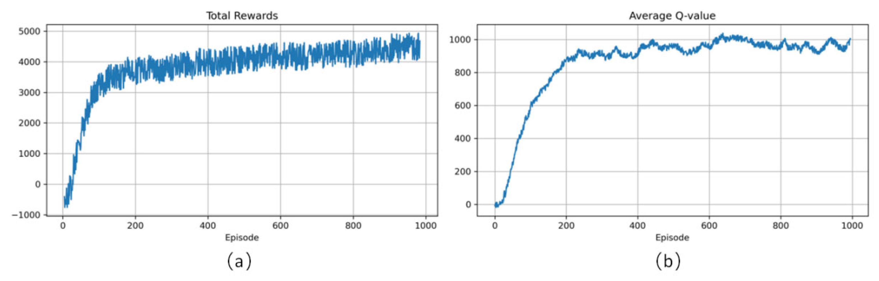
This study addresses the path planning challenges of lunar rovers in complex dynamic environments by proposing an A*-D3QN-Opt method that integrates digital twin technology with improved deep reinforcement learning. By constructing a hierarchical path planning architecture, optimizing deep reinforcement learning algorithms, and designing a multimodal perception system, the study achieves efficient navigation of the lunar rover under multiple constraints. The proposed A*-D3QN-Opt method significantly improves path planning efficiency and robustness through a synergistic mechanism of static global planning and dynamic local adjustments. The A* algorithm provides prior knowledge of the globally optimal path for deep reinforcement learning, effectively alleviating the exploration blindness (when the lunar rover performs path exploration in a complex and dynamic environment, due to the absence of effective prior knowledge or global guidance, its exploration behavior demonstrates blindness and inefficiency) inherent in reinforcement learning in complex environments. The improved D3QN algorithm, through a quintuple reward function and prioritized experience replay mechanism, enhances the rover’s real-time response capability to dynamic obstacles and sudden environmental changes. Experiments show that the method reduces path lengths by 50.7%, 24.2%, and 26.3% in low-, medium-, and high-complexity environments, respectively, compared to the traditional D3QN, verifying the superiority of the hierarchical architecture. The improved D3QN algorithm achieves multi-objective optimization through the quintuple reward function (path progress, obstacle avoidance, direction, energy consumption, and time penalty), successfully reducing collision counts to zero in high-complexity environments and increasing the average Q-value to 299.87. The prioritized experience replay mechanism, by dynamically adjusting the weight of experience samples, accelerates model convergence by approximately 30%, reducing training time by one hour in medium-complexity environments. The YOLOv5-DisNet multimodal perception system improves target detection accuracy by 15%, with distance estimation errors controlled within ±5%, providing reliable environmental information for path planning. The constructed digital twin model achieves high-fidelity mapping of lunar terrain, motion control, and task constraints, providing a safe and controllable simulation training environment for reinforcement learning. Through virtual-real interaction validation, the lunar rover, after completing 1000 training episodes in the virtual environment, quickly adapts to dynamic changes in real-world scenarios, significantly reducing trial-and-error costs in actual missions. This research provides an innovative solution for lunar rover path planning, although there is still room for improvement. Future work will focus on the development of multi-rover collaborative path planning algorithms and enhancing model robustness in extreme environments such as lunar nights with low temperatures and high radiation.